Novel approach to neutron electric dipole moment search using weak measurement

Abstract

We propose a novel approach in a search for the neutron electric dipole moment (EDM) by taking advantage of signal amplification in a weak measurement, known as weak value amplification. Considering an analogy to the weak measurement that can measure the spin magnetic moment interaction, we examine an experimental setup with a polarized neutron beam through an external electric field with spatial gradient, where the signal is sensitive to the EDM interaction. In particular, a dedicated analysis of effects from impurities in pre- and post-selections is performed. We show that the weak value amplification occurs where the signal is enhanced by up to two orders of magnitude, and demonstrate a potential sensitivity of the proposed setup to the neutron EDM.

I Introduction

Since $CP$ violation arises from only the phase of the Cabibbo-Kobayashi-Maskawa matrix in the standard model (SM) and it is tiny Kobayashi and Maskawa (1973), $CP$-violating observables have provided good measurement sensitive to physics beyond the SM. In particular, measurement of the electric dipole moment (EDM) of the neutron, $d_{\rm n}$, can give a clear signal of new physics (NP), and has been a big subject for the last seventy years Ramsey (1982).

The neutron EDM arises from three-loop short-distance Shabalin (1978); Khriplovich (1986); Czarnecki and Krause (1997), two-loop long-distance Khriplovich and Zhitnitsky (1982); McKellar et al. (1987), one-loop contributions from the QCD theta term Dragos et al. (2021), and tree-level charm-quark contributions Mannel and Uraltsev (2012) within the SM, while it can arise from one-loop diagrams in general NP models, such as multi-Higgs bosons Weinberg (1976); Deshpande and Ma (1977); Weinberg (1989); Barr and Zee (1990), supersymmetric particles Ellis et al. (1982); Buchmuller and Wyler (1983); Polchinski and Wise (1983); Dugan et al. (1985), leptoquark Arnold et al. (2013); Fuyuto et al. (2019); Dekens et al. (2019), and models with dynamical electroweak symmetry breaking Appelquist et al. (2004a, b). In addition, observed matter-antimatter asymmetry in the Universe requires new $CP$-violating sources Sakharov (1967); Gavela et al. (1994), which could be verified by the measurement of the EDM, e.g., Ref. Fuyuto et al. (2016).

So far, although much effort has been devoted to search for the EDMs, they have not been observed yet. One of the most severe limits comes from the neutron EDM search Pendlebury et al. (2015)

$$(d_{\rm n})_{\rm exp}<3.0\times 10^{-26}~{}e\,{\rm cm}~{}(90\%~{}{\rm CL})\,,$$ (1)

by measuring a neutron resonant frequency of ultracold neutrons (UCNs) based on the separated oscillatory field method (the so-called Ramsey method) Ramsey (1949, 1950). This limit is five orders of magnitude larger than the SM prediction $(d_{\rm n})_{\rm SM}\sim 10^{-(31\textrm{--}32)}~{}e\,{\rm cm}$ Khriplovich and Zhitnitsky (1982); McKellar et al. (1987); Mannel and Uraltsev (2012). Nevertheless, it severely constrains the NP scenarios that include additional $CP$ violation.

In the early stage of the neutron EDM experiments, not the UCNs but a polarized neutron beam had been utilized Smith et al. (1957); Baird et al. (1969); Dress et al. (1977a); Ramsey (1986). However, it was known that there was a large systematic uncertainty in neutron beam experiment which comes from relativistic effects. The relativistic effects arise from the motion of neutrons (velocity ${\bf v}$) through the electric field ${\bf E}$, as (see, e.g., Ref. Feynman et al. (1964) for a derivation)

$${\bf B}=\frac{{\bf E}\times{\bf v}}{c^{2}}\,.$$ (3)

Even if the neutron beam is shielded from the external magnetic field which we will assume in this paper, the external electric field does generate the magnetic filed depending on the velocity (it can be interpreted as the relativistic transformation of $F_{\mu\nu}$), and the sensitivity of the experiment becomes dull because of the large spin magnetic moment interaction.

In order to avoid large uncertainties, current experiments and new proposed projects are using the UCNs Altarev et al. (1996); Baker et al. (2006); Ito (2007); van der Grinten et al. (2009); Serebrov et al. (2009); Lamoreaux and Golub (2009); Baker et al. (2011); Masuda et al. (2012); Altarev et al. (2012). Moreover, most of the experiments have employed the Ramsey method Ramsey (1949, 1950). The main reasons why the UCNs are preferred are the following two Piegsa (2013): First, the systematic uncertainty from the relativistic effects can be neglected because of its small velocity of the UCNs. Second, the UCNs can have longer interaction times with the external electric field because they can be trapped easily, and the statistical uncertainty is suppressed.

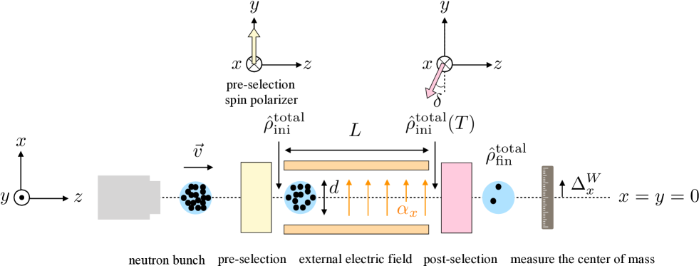
Figure 1: Schematic drawing of the proposed experimental setup. First, emitted neutron bunches from neutron source (the leftmost gray box) are polarized into the yellow arrow in the first polarizer (the yellow box) and it is called pre-selection. The initial state in this paper is a neutron state that just goes through the first polarizer. After the pre-selection, the neutron bunches go through the external electric field with spatial gradient along $x$ axis for a distance $L\,(=vT)$. Then, the neutron bunches are selected by the second polarizer (the pink box) where a specific spin polarization state (the pink allow) can pass. The final state is a neutron state that just goes through the post-selection. After the post-selection, the detector measures a position of the center-of-mass of the neutron bunch. Spin directions of the two polarizers are exhibited above the polarizers. The black dots in the neutron bunch roughly represent the single neutron: the number of neutron significantly decreases after the post-selection.

On the other hand, in the polarized neutron beam experiments, although severe systematic effects come from the relativistic ${\bf E}\times{\bf v}$ corrections Dress et al. (1977a); Piegsa (2013), one can prepare a much larger amount of neutrons, which can reduce statistical fluctuations. Also, one can use stronger external electric fields, because the neutron beams are not covered by an insulating wall unlike the UCNs. Besides, there are several ideas that the relativistic ${\bf E}\times{\bf v}$ corrections can be suppressed in the neutron beam experiments with the Ramsey method Piegsa (2013) or with a spin rotation in non-centrosymmetric crystals Fedorov et al. (2005, 2008, 2009a, 2009b). The latter idea has been realized in an experiment Fedorov et al. (2011).

In this paper, we propose a novel experimental approach in the search for the neutron EDM by applying not the Ramsey method but a method of weak measurement Aharonov et al. (1964, 1988); Lee and Tsutsui (2014), and discuss conditions how our setup can overtake the current upper limit in Eq. (1). This work is the first application of the weak measurement to the neutron EDM measurement. For instance, the spin magnetic moment interaction had been measured by the weak measurement Aharonov et al. (1988); Sponar et al. (2015), where a tremendous amplification of signal (a component of a spin) emerged. Also, the weak measurement using an optical polarizer with a laser beam has been realised Ritchie et al. (1991); Pryde et al. (2005). We also show that the relativistic ${\bf E}\times{\bf v}$ corrections are suppressed in this approach.

In the weak measurement, two quantum systems are prepared, and then the initial and final states are properly selected in one of the quantum systems, which are called pre- ($|\psi_{i}\rangle$) and post-selections ($\langle\psi_{f}|$), respectively. A weak value, corresponding to an observable $\hat{A}$, is defined as

$$\langle\hat{A}\rangle^{W}\equiv\frac{\langle\psi_{f}|\hat{A}|\psi_{i}\rangle}{\langle\psi_{f}|\psi_{i}\rangle}\in\mathbb{C}\,,$$ (4)

and can be amplified by choosing the proper selections of the states: $\langle\psi_{f}|\psi_{i}\rangle\sim 0$, which is called weak value amplification (for reviews see, e.g., Refs. Aharonov et al. (2010); Kofman et al. (2012)). Since the weak value is obtained as an observable quantity corresponding to $\hat{A}$ in an intermediate measurement between $|\psi_{i}\rangle$ and $\langle\psi_{f}|$ without disturbing the quantum systems, measurement of the weak value plays an important role in the quantum mechanics itself. In addition, the weak value provides new methods for precise measurements Aharonov and Vaidman (1991); Yokota et al. (2009). In fact, the weak value amplification was applied to precise measurements such as the spin Hall effect of the light (four orders of magnitude amplified) Hosten and Kwiat (2008) and the beam deflection in a Sagnac interferometer (two orders of magnitude amplified) Dixon et al. (2009).

In our setup (see Fig. 1), as explained in details at the next section, unlike the Ramsey method with using the UCN, we consider a polarized neutron beam with the velocity of $\sim 10^{3}~{}{\rm m/sec}$. We investigate the motion of a neutron bunch in the external electric field with spatial gradient, and apply methods of the weak measurement which leads to amplification of the signal.

Very interestingly, it will be shown in our setup that the systematic uncertainty from the relativistic ${\bf E}\times{\bf v}$ effect can be irrelevant compared to a neutron EDM signal. This fact is expected as a new virtue of the weak measurement because our finding implies that the weak measurement itself is useful in quantum systems to suppress the systematic uncertainty such as the relativistic effect.

This paper is organized as follows. In Sec. II, we propose an experimental setup for the neutron EDM search using the weak measurement. In Sec. III, we analytically calculate an expected observable in this setup. Especially, the weak value is introduced. Numerical results are evaluated in Sec. IV. We will show the weak value amplification and a potential sensitivity to the neutron EDM signal in this setup. Finally, Sec. V is devoted for the conclusions. In Appendix A, a general setup of an external electric field is considered. In Appendix B, a formalism of a full-order calculation of the expected observable is provided.

II Experimental setup

We consider application of the weak measurement method Aharonov et al. (1988) to the neutron EDM measurement. Because Ref. Aharonov et al. (1988) utilizes an external magnetic field with a spatial gradient for measuring the spin magnetic moment, one should use the polarized neutron beam and an external electric field with a spatial gradient.

In order to obtain a signal amplification in a weak measurement (weak value amplification), two important selections are necessary: the pre-selection and the post-selection. The pre-selection is equivalent to preparation of the initial state in the conventional quantum mechanics. On the other hand, the post-selection is extraction of a specific quantum state at the late time Aharonov et al. (1964), and it makes to understand the weak value amplification difficult because of lack of counterparts in the conventional quantum mechanics. In a nutshell, the role of the post-selection is filtering where only events that the observable (such as the position of the neutron) takes a large value are collected. Note that the weak value amplification originates from the quantum interference Duck et al. (1989); Vaidman (2014); Dressel (2015); Qin et al. (2016), so that classical filtering is not suitable. In our setup, we impose selections of the spin polarization of the neutrons as the pre- and post-selections.

Figure 1 shows our proposed experimental setup. The detailed explanation is given in the figure caption and the following paragraph, especially the electric field with the spatial gradient $\alpha_{x}$ is represented by the orange arrows. We set $xyz$ axis as follows: The neutrons fly along the $z$ axis. The external electric field has the gradient along $x$ axis. A spin direction of the pre-selection at the first spin polarizer is $y$ axis.

The entire process of the setup is divided into four stages:

1. Pre-selection. At $t=0$, the neutron bunch emitted from the neutron source is polarized at the first polarizer (the yellow box in Fig. 1), and the quantum state of the total system is represented by the following density matrices

   $$\hat{\rho}^{\rm total}_{\rm ini}=\hat{\rho}^{P}_{\rm ini}\otimes\hat{\rho}^{S}_{\rm ini}\,,$$ (5)

   where $\hat{\rho}^{P}_{\rm ini}$ is the initial state of the neutron position and $\hat{\rho}^{S}_{\rm ini}$ is the pre-selected spin polarization.

2. Time evolution in external electric field. For $0<t<T$, the neutron bunch goes through the external electric field with spatial gradient in Fig. 1, where the total system evolves by the Hamiltonian Eq. (9) as

   $$\hat{\rho}^{\rm total}_{\rm ini}(t)=e^{-i\hat{H}t}\hat{\rho}^{\rm total}_{\rm ini}e^{i\hat{H}t}\,.$$ (6)

   Note that in this paper, although we do not use the natural units, $\hbar$ is discarded for simplicity.

3. Post-selection. After the time evolution of the total system in the external electric field, at $t=T$, the neutrons are selected in the second polarizer (the pink box in Fig. 1) where a specific spin polarization state ($\hat{\rho}^{S}_{\rm fin}$) of the neutron can pass. Then, the neutron position is represented by a density matrix

   $$\hat{\rho}^{P}_{\rm fin}={\rm Tr}_{S}\left[\hat{\rho}^{S}_{\rm fin}\hat{\rho}^{\rm total}_{\rm ini}(T)\right]\,.$$ (7)

4. Measurement of the center of mass. After the post-selection, position shifts of the neutron along $x$-axis are measured. Here, by taking the average of those shifts, one can measure a position shift of the center-of-mass of the neutrons passing the post-selection. The expectation value of the position shift is expressed as

   $$\Delta^{W}_{x}=\frac{{\rm Tr}_{P}\left[\hat{x}\hat{\rho}^{P}_{\rm fin}\right]}{{\rm Tr}_{P}\left[\hat{\rho}^{P}_{\rm fin}\right]}\,.$$ (8)

The detail evaluations of these processes will be discussed in the next section.

The external electric field is set between the pre-selection and the post-selection. As discussed in Appendix A, one can define the $x$ axis as the direction of spatial gradient of the external electric field. Therefore, $x$ dependence of $y$ and $z$ components of the external electric field is negligible without loss of generality. According as the size of the neutron EDM and the spin polarization, displacement of the neutron along $x$ axis occurs. We would like to maximize this displacement by the weak value amplification.

In this setup, the single neutron can be described by the non-relativistic Hamiltonian Pospelov and Ritz (2005):

$$\hat{H}=\frac{\hat{\bf p}^{2}}{2m_{\rm n}}-d_{\rm n}\hat{\bf E}\cdot\hat{\bm{\sigma}}-\frac{\mu_{\rm n}}{m_{\rm n}c^{2}}(\hat{\bf E}\times\hat{\bf p})\cdot\hat{\bm{\sigma}}\,,$$ (9)

where $\hat{\bf p}$ is the momentum operator of a neutron, $m_{\rm n}$ is the neutron mass, $d_{\rm n}$ is the neutron EDM, $\mu_{\rm n}$ is the neutron magnetic moment, $\hat{\bf E}$ is an operator of the external electric field vector, and $\hat{\bm{\sigma}}$ is the spin operator corresponding to the polarized neutron: the operation on spin-states is defined as $\hat{\sigma}_{i}\left|{\pm}_{i}\right>=\pm\left|{\pm}_{i}\right>~{}{\rm for~{}}i=x,y,z$. This Hamiltonian is defined in the Hilbert space $\mathcal{H}=\mathcal{H}_{P}\otimes\mathcal{H}_{S}$, where $\mathcal{H}_{P}$ is the Hilbert space of the position ($P$) of the neutron, while $\mathcal{H}_{S}$ is that of the spin ($S$) of the neutron. Note that although the external magnetic field is zero in the setup, the magnetic filed is generated by the relativistic effect in Eq. (3).

III Weak measurement

In this section, we derive an analytic formula of an expectation value of deviation of the neutron position from $x=0$, which is shown as $\Delta_{x}^{W}$ in Fig. 1.

To analytically study our strategy for the neutron EDM search based on the weak value amplification, we adopt two assumptions as follows:

Assumption 1: We consider the following external electric field operator:

$$\hat{\bf E}=\left(E_{x}^{0}+\alpha\hat{x},\ E_{y}^{0},\ 0\right)\,,$$ (10)

where $E_{x}^{0},\,E_{y}^{0}$, and $\alpha$ are constants (namely $\alpha=dE_{x}/dx$). $\hat{x}$ is an operator corresponding to the $x$ coordinate of the neutron. A necessary condition of this form is discussed in Appendix A. Even if the $E_{z}$ component is nonzero, the effect is irrelevant in this setup. Although $E_{z}$ generates $B_{x,y}$ via the relativistic effects in the third terms of Eq. (9), they are significantly suppressed by small neutron momenta, $v_{x}$ and $v_{y}$.

Assumption 2: We consider the following neutron initial state in the Hilbert space $\mathcal{H}_{P}$:

$$\hat{\rho}^{P}_{\rm ini} \equiv\left|G_{p_{x0}}\otimes p_{y0}\otimes p_{z0}\right>\left<G_{p_{x0}}\otimes p_{y0}\otimes p_{z0}\right|,$$ (11)

where we defined as

$$\langle x|G_{p_{x0}}\rangle =\frac{1}{(2\pi d^{2})^{1/4}}e^{ip_{x0}\cdot x}e^{-\frac{x^{2}}{4d^{2}}}\,,$$ (12)

$$\langle j|p_{j0}\rangle =\frac{1}{\sqrt{2\pi}}e^{ip_{j0}\cdot j}\,,\quad\textrm{for~{}}j=y,\,z\,.$$ (13)

Here, $p_{x0},\,p_{y0}$ and $p_{z0}$ are the initial neutron momenta, and ${|G_{p_{x0}}\rangle},\,{|p_{y0}\rangle}$ and ${|p_{z0}\rangle}$ are the quantum states of $x,\,y$ and $z$ directions, respectively. We are interested in the spatial displacement of the neutron along $x$ axis. As explained below, in the weak measurement, the expectation value of the neutron position depends on only variance of the distribution. Therefore, we assume the Gaussian wave packet $|G\rangle$ as the a quantum state of $x$ direction, for simplicity Ishikawa and Shimomura (2006); Ishikawa and Oda (2018). In the distribution, we regard $d$ as a standard deviation of the neutron beam and assume that the neutron beam diameter is $2d$ for the $x$ direction. On the other hand, for $y$ and $z$ directions, we assume the plane wave.

In addition to above assumptions, we use several numerical approximations in this section. These approximation are reasonable when one takes input values which will be used in Sec. IV. Note that these numerical approximations are not used in the final plot of Sec. IV.

Based on the assumption 1 in Eq. (10), the Hamiltonian in Eq. (9) can be expressed as

$$\hat{H}= \frac{\hat{\bf p}^{2}}{2m_{\rm n}}-g_{\mu}\left[\chi\left(E_{x}^{0}+\alpha\hat{x}\right)+E_{y}^{0}\hat{n}_{p_{z}}\right]\otimes\hat{\sigma}_{x}$$

$$-g_{\mu}\left[\chi E_{y}^{0}-\left(E_{x}^{0}+\alpha\hat{x}\right)\hat{n}_{p_{z}}\right]\otimes\hat{\sigma}_{y}$$

$$-g_{\mu}\left[\left(E_{x}^{0}+\alpha\hat{x}\right)\hat{n}_{p_{y}}-E_{y}^{0}\hat{n}_{p_{x}}\right]\otimes\hat{\sigma}_{z},$$ (14)

where we defined $p_{0}\equiv\sqrt{p_{x0}^{2}+p_{y0}^{2}+p_{z0}^{2}}$, $g_{\mu}\equiv\mu_{\rm n}p_{0}/(m_{\rm n}c^{2})$, $\chi\equiv d_{\rm n}/g_{\mu}$, and $\hat{n}_{p_{i}}\equiv\hat{p}_{i}/p_{0}$ ($i=x,\,y,\,z$) for convenience in the following analysis. All interactions are normalized by $g_{\mu}$, and the EDM interaction is represented as $\chi g_{\mu}$. Note that $\chi$ is dimensionless real quantity.

The time evolution operator is $e^{-i\hat{H}t}$. Using the Baker–Campbell–Hausdorff formula, and $[\hat{x},\hat{p}_{x}]=i$ and $[\hat{x},\hat{p}^{2}_{x}]=2i\hat{p}_{x}$, we obtain

$$\exp\left(-i\hat{H}t\right)=\exp\left(-i\frac{\hat{\bf p}^{2}}{2m_{\rm n}}t\right)\exp\left[-i\left(\hat{H}_{0}+\hat{H}_{\chi}\right)t+\mathcal{O}\left(t^{3}g^{2}_{\mu}\frac{\alpha^{2}}{m_{\rm n}}\,,t^{3}g^{2}_{\mu}\alpha E_{y}^{0}\frac{\hat{p}_{x}}{m_{\rm n}}\right)\right]\,,$$ (15)

where the interaction Hamiltonian with the background ($\hat{H}_{0}$) and with the EDM ($\hat{H}_{\chi}$) are

$$\hat{H}_{0}\equiv-g_{\mu}E_{x}^{0}\left[\frac{E_{y}^{0}}{E_{x}^{0}}\hat{n}_{p_{z}}\otimes\hat{\sigma}_{x}-\hat{n}_{p_{z}}\otimes\hat{\sigma}_{y}+\left(\hat{n}_{p_{y}}-\frac{E_{y}^{0}}{E_{x}^{0}}\hat{n}_{p_{x}}\right)\otimes\hat{\sigma}_{z}\right]+g_{\mu}\alpha\left(\hat{x}+\frac{t}{2m_{\rm n}}\hat{p}_{x}\right)\left(\hat{n}_{p_{z}}\otimes\hat{\sigma}_{y}-\hat{n}_{p_{y}}\otimes\hat{\sigma}_{z}\right)\,,$$ (16)

$$\hat{H}_{\chi}\equiv-\chi g_{\mu}\left[E_{x}^{0}+\alpha\left(\hat{x}+\frac{t}{2m_{\rm n}}\hat{p}_{x}\right)\right]\otimes\hat{\sigma}_{x}-\chi g_{\mu}E_{y}^{0}\otimes\hat{\sigma}_{y}\,.$$ (17)

We have checked that the $\mathcal{O}(t^{3})$ terms in Eq. (15) are numerically negligible in the following analysis. Moreover, the last term in Eq. (17) is totally screened by $g_{\mu}E_{x}^{0}\hat{n}_{p_{z}}\otimes\hat{\sigma}_{y}$ in $\hat{H}_{0}$.

Then, we expand the interaction Hamiltonian by $\alpha\hat{x}$, and obtain the following analytic form:

$$\exp\left[-i\left(\hat{H}_{0}+\hat{H}_{\chi}\right)t\right]=\hat{U}_{0}(t)+\alpha\left(\hat{x}+\frac{t}{2m_{\rm n}}\hat{p}_{x}\right)\!\hat{U}_{1}(t)+\mathcal{O}\left(\alpha^{2}\left(\hat{x}+\frac{t}{2m_{\rm n}}\hat{p}_{x}\right)^{2}\right)\,,$$ (18)

with

$$\hat{U}_{0}(t)= I_{2}\cos\left(g_{\mu}E_{x}^{0}t\right)+\begin{pmatrix}-i\frac{E_{y}^{0}}{E_{x}^{0}}n_{p_{x0}}+in_{p_{y0}}&-n_{p_{z0}}+i\frac{E_{y}^{0}}{E_{x}^{0}}n_{p_{z0}}+i\chi\\ n_{p_{z0}}+i\frac{E_{y}^{0}}{E_{x}^{0}}n_{p_{z0}}+i\chi&+i\frac{E_{y}^{0}}{E_{x}^{0}}n_{p_{x0}}-in_{p_{y0}}\end{pmatrix}\sin\left(g_{\mu}E_{x}^{0}t\right)+\mathcal{O}\left(\left(\frac{E_{y}^{0}}{E_{x}^{0}}\right)^{2}\right)\,,$$ (19)

$$\hat{U}_{1}(t)= \begin{pmatrix}-i\frac{E_{y}^{0}}{E_{x}^{0}}n_{p_{x0}}+in_{p_{y0}}&i\frac{E_{y}^{0}}{E_{x}^{0}}n_{p_{z0}}-n_{p_{z0}}+i\chi\\ i\frac{E_{y}^{0}}{E_{x}^{0}}n_{p_{z0}}+n_{p_{z0}}+i\chi&i\frac{E_{y}^{0}}{E_{x}^{0}}n_{p_{x0}}-in_{p_{y0}}\end{pmatrix}g_{\mu}t\cos\left(g_{\mu}E_{x}^{0}t\right)$$

$$+\begin{pmatrix}i\frac{E_{y}^{0}}{(E_{x}^{0})^{2}}n_{p_{x0}}-g_{\mu}t&-i\frac{E_{y}^{0}}{(E_{x}^{0})^{2}}n_{p_{z0}}\\ -i\frac{E_{y}^{0}}{(E_{x}^{0})^{2}}n_{p_{z0}}&-i\frac{E_{y}^{0}}{(E_{x}^{0})^{2}}n_{p_{x0}}-g_{\mu}t\end{pmatrix}\sin\left(g_{\mu}E_{x}^{0}t\right)+\mathcal{O}\left(\left(\frac{E_{y}^{0}}{E_{x}^{0}}\right)^{2}\right)\,,$$ (20)

where $I_{2}$ is the $2\times 2$ unit matrix. Hereafter, we assume $\hat{n}_{p_{i}}\to n_{p_{i0}}=p_{i0}/p_{0}~{}(i=x,\,y,\,z)$ and $n_{p_{x0}}^{2}+n_{p_{y0}}^{2}+n_{p_{z0}}^{2}=1$ for simplicity of calculations. The higher-order terms $\mathcal{O}((E_{y}^{0}/E_{x}^{0})^{2})$ are numerically irrelevant when $E_{y}^{0}\ll E_{x}^{0}$. The $\hat{U}_{0}(t)$ and $\hat{U}_{1}(t)$ satisfy the unitarity condition:

$$\hat{U}_{0}(t)\hat{U}_{0}(t)^{{\dagger}}=I_{2}\,,~{}~{}~{}\hat{U}_{1}(t)\hat{U}_{1}(t)^{{\dagger}}=\left(g_{\mu}t\right)^{2}I_{2}\,,~{}~{}~{}\hat{U}_{0}(t)\hat{U}_{1}(t)^{{\dagger}}+\hat{U}_{1}(t)\hat{U}_{0}(t)^{{\dagger}}=0\,,$$ (21)

up to the following higher-order corrections:

$$\mathcal{O}\left(\chi\frac{E_{y}^{0}}{E_{x}^{0}},\,\chi^{2},\,\left(\frac{E_{y}^{0}}{E_{x}^{0}}\right)^{2},\,n_{p_{x0}}^{2},\,\frac{E_{y}^{0}}{E_{x}^{0}}n_{p_{x0}}n_{p_{y0}}\right)\,.$$ (22)

Now, we obtain the compact form of the time evolution operator,

$$\exp\left(-i\hat{H}t\right)\simeq\exp\left(-i\frac{\hat{\bf p}^{2}}{2m_{\rm n}}t\right)\left[\hat{U}_{0}(t)+\alpha\left(\hat{x}+\frac{t}{2m_{\rm n}}\hat{p}_{x}\right)\!\hat{U}_{1}(t)\right]\,.$$ (23)

As mentioned previous section, the weak measurement requires pre- and post-selections, and we select the neutron spin polarization. Since the neutron polarization rate is not perfect in practical spin polarizers, we include an impurity effect in the pre- and post-selections as mixed spin states of the neutron. As will be shown later, the final result significantly depends on the impurity effect. This is because neutron passing probability at the post-selection is sensitive to the impurity effect in this setup, and large passing probability dulls the neutron position shift. We consider the following pre-selected state in the Hilbert space $\mathcal{H}_{S}$:

$$\hat{\rho}^{S}_{\rm ini} =(1-\epsilon){|\psi\rangle}{\langle\psi|}+\epsilon{|\phi\rangle}{\langle\phi|}$$

$$=\frac{1}{2}\begin{pmatrix}1&-i(1-2\epsilon)\\ i(1-2\epsilon)&1\end{pmatrix}\,,$$ (24)

where two polarization states are (see Fig. 1)

$${|\psi\rangle} ={|+_{y}\rangle}=\frac{1}{\sqrt{2}}\begin{pmatrix}i\\ -1\end{pmatrix}\,,$$ (25)

$${|\phi\rangle} ={|-_{y}\rangle}=\frac{1}{\sqrt{2}}\begin{pmatrix}i\\ 1\end{pmatrix}\,.$$ (26)

Here, ${|\pm_{y}\rangle}$ are eigenstates of the spin operator $\hat{\sigma}_{y}$, and $\epsilon$ $(0<\epsilon\ll 1)$ stands for the selection impurity.

After the pre-selection, the quantum state of the total system at the initial time $t=0$ can be expressed as direct-product $\hat{\rho}_{\rm ini}^{\rm total}=\hat{\rho}^{P}_{\rm ini}\otimes\hat{\rho}^{S}_{\rm ini},$ where $\hat{\rho}^{P}_{\rm ini}$ is defined in Eq. (11), which is the assumption 2.

The late-time quantum state of the total system at $t=T$ (see Fig. 1) just before the post-selection is given as

$$\hat{\rho}_{\rm ini}^{\rm total}(T)=e^{-i\hat{H}T}\hat{\rho}_{\rm ini}^{\rm total}e^{i\hat{H}T}$$

$$=e^{-i\frac{\hat{\bf p}^{2}}{2m_{\rm n}}T}\left[\hat{U}_{0}(T)+\alpha\left(\hat{x}+\frac{T}{2m_{\rm n}}\hat{p}_{x}\right)\!\hat{U}_{1}(T)\right]\hat{\rho}_{\rm ini}^{\rm total}\left[\hat{U}_{0}(T)^{{\dagger}}+\alpha\left(\hat{x}+\frac{T}{2m_{\rm n}}\hat{p}_{x}\right)\!\hat{U}_{1}(T)^{{\dagger}}\right]e^{i\frac{\hat{\bf p}^{2}}{2m_{\rm n}}T}\,.$$ (27)

Next, we consider the following post-selected state:

$$\hat{\rho}^{S}_{\rm fin} =(1-\epsilon){|\phi_{\delta}\rangle}{\langle\phi_{\delta}|}+\epsilon{|\psi_{\delta}\rangle}{\langle\psi_{\delta}|}$$

$$=\frac{1}{2}\begin{pmatrix}1+(1-2\epsilon)\sin\delta&i(1-2\epsilon)\cos\delta\\ -i(1-2\epsilon)\cos\delta&1-(1-2\epsilon)\sin\delta\end{pmatrix}\,,$$ (28)

with

$${|\psi_{\delta}\rangle} \equiv e^{i\frac{\delta}{2}\hat{\sigma}_{x}}{|+_{y}\rangle}=\frac{1}{\sqrt{2}}\begin{pmatrix}i\left(\cos\frac{\delta}{2}-\sin\frac{\delta}{2}\right)\\ -\left(\cos\frac{\delta}{2}+\sin\frac{\delta}{2}\right)\end{pmatrix}\,,$$

$${|\phi_{\delta}\rangle} \equiv e^{i\frac{\delta}{2}\hat{\sigma}_{x}}{|-_{y}\rangle}=\frac{1}{\sqrt{2}}\begin{pmatrix}i\left(\cos\frac{\delta}{2}+\sin\frac{\delta}{2}\right)\\ \cos\frac{\delta}{2}-\sin\frac{\delta}{2}\end{pmatrix}\,.$$ (29)

Here, $\delta$ is a polarization angle around $x$-axis for the post-selection (see Fig. 1). It is known that small $\delta$ angle is preferred for the weak value amplification Aharonov et al. (1988). The selection impurity $\epsilon$ is also included in the post-selection, and we assume its quality is the same as the pre-selection, for simplicity.

After the post-selection, the final state of the total system is written as $\hat{\rho}_{\rm fin}^{\rm total}=\hat{\rho}^{P}_{\rm fin}\otimes\hat{\rho}^{S}_{\rm fin}.$ Using the late-time state in Eq. (27), we obtain the neutron final state in the Hilbert space $\mathcal{H}_{P}$,

$$\hat{\rho}^{P}_{\rm fin}\equiv {\rm Tr}_{S}\left[\hat{\rho}_{\rm fin}^{\rm total}\right]={\rm Tr}_{S}\left[\hat{\rho}^{S}_{\rm fin}\hat{\rho}^{\rm total}_{\rm ini}(T)\right]$$

$$= {\rm Tr}_{S}\left[\hat{\rho}^{S}_{\rm fin}\hat{U}_{0}(T)\hat{\rho}^{S}_{\rm ini}\hat{U}_{0}(T)^{\dagger}\right]e^{-i\frac{\hat{\bf p}^{2}}{2m_{\rm n}}T}\left\{\hat{\rho}^{P}_{\rm ini}+\chi g_{\mu}\alpha T\left[W\hat{\rho}^{P}_{\rm ini}\left(\hat{x}+\frac{T}{2m_{\rm n}}\hat{p}_{x}\right)+W^{\ast}\left(\hat{x}+\frac{T}{2m_{\rm n}}\hat{p}_{x}\right)\hat{\rho}^{P}_{\rm ini}\right]\right\}e^{i\frac{\hat{\bf p}^{2}}{2m_{\rm n}}T}$$

$$+\mathcal{O}\left(\left(g_{\mu}\alpha T\right)^{2}\right)\,,$$ (30)

where we defined the following dimensionless complex quantity $W$,

$$W\equiv\frac{1}{\chi g_{\mu}T}\frac{{\rm Tr}_{S}\left[\hat{\rho}^{S}_{\rm fin}\hat{U}_{0}(T)\hat{\rho}^{S}_{\rm ini}\hat{U}_{1}(T)^{\dagger}\right]}{{\rm Tr}_{S}\left[\hat{\rho}^{S}_{\rm fin}\hat{U}_{0}(T)\hat{\rho}^{S}_{\rm ini}\hat{U}_{0}(T)^{\dagger}\right]}\,.$$ (31)

The $W$ corresponds to the weak value. For the third term of Eq. (30), using Eqs. (24) and (28), we used

$${\rm Tr}_{S}\left[\hat{\rho}^{S}_{\rm fin}\hat{U}_{1}(T)\hat{\rho}^{S}_{\rm ini}\hat{U}_{0}(T)^{\dagger}\right] ={\rm Tr}_{S}\left[\hat{U}_{0}(T)^{\ast}(\hat{\rho}^{S}_{\rm ini})^{T}\hat{U}_{1}(T)^{T}(\hat{\rho}^{S}_{\rm fin})^{T}\right]$$

$$={\rm Tr}_{S}\left[\hat{\rho}^{S}_{\rm fin}\hat{U}_{0}(T)\hat{\rho}^{S}_{\rm ini}\hat{U}_{1}(T)^{\dagger}\right]^{\ast}\,.$$ (32)

Similarly, one can easily find ${\rm Tr}_{S}\left[\hat{\rho}^{S}_{\rm fin}\hat{U}_{0}(T)\hat{\rho}^{S}_{\rm ini}\hat{U}_{0}(T)^{\dagger}\right]={\rm Tr}_{S}\left[\hat{\rho}^{S}_{\rm fin}\hat{U}_{0}(T)\hat{\rho}^{S}_{\rm ini}\hat{U}_{0}(T)^{\dagger}\right]^{\ast}=$ real.

In an ideal experimental setup limit, $E_{y}^{0}/E_{x}^{0}\to 0$, $n_{p_{x0,y0}}\to 0$, and $\epsilon\to 0$, the weak value $W$ is expressed as

$$W =-i\frac{\langle{\psi(T)|\hat{\sigma}_{x}|\phi_{\delta}\rangle}}{\langle{\psi(T)|\phi_{\delta}\rangle}}+\frac{i}{\chi}\frac{\langle{\psi(T)|\hat{\sigma}_{y}|\phi_{\delta}\rangle}}{\langle{\psi(T)|\phi_{\delta}\rangle}}$$ (33)

$$=\frac{i}{\chi}-e^{-2ig_{\mu}E_{x}^{0}T}\cot\left(\frac{\delta}{2}\right)+\mathcal{O}(\chi)\,,$$ (34)

where we define

$${|\psi(T)\rangle} =\hat{U}_{0}(T){|\psi\rangle}$$

$$=\left\{\cos\left(g_{\mu}E_{x}^{0}T\right)I_{2}+i\sin\left(g_{\mu}E_{x}^{0}T\right)\left[\chi\hat{\sigma}_{x}-\hat{\sigma}_{y}\right]\right\}{|\psi\rangle}$$ (35)

$$=e^{-ig_{\mu}E_{x}^{0}T}{|\psi\rangle}+i\sin\left(g_{\mu}E_{x}^{0}T\right)\chi\hat{\sigma}_{x}{|\psi\rangle}\,.$$ (36)

According to the definition of the weak value in Eq. (4), we find $W=-i\langle\hat{\sigma}_{x}\rangle^{W}+\frac{i}{\chi}\langle\hat{\sigma}_{y}\rangle^{W}$ in the ideal experimental limit, and show that $W$ is amplified by $\cot(\delta/2)$ for small $\delta$ region Aharonov et al. (1988). One should note that since $W$ is always multiplied by $\chi$ in Eq. (30), the first term in Eq. (34) is not singular in $\chi\to 0$ limit. In other words, there is a contribution in Eq. (30) that is independent of $\chi$ (signal) and sensitive to the weak value $W$, especially $\langle\hat{\sigma}_{y}\rangle^{W}$. We will show that such a contribution corresponds to a background effect (from the relativistic ${\bf E}\times{\bf v}$ effect). It would be interesting possibility to measure the weak value from the background effect, even if one cannot measure the neutron EDM signal. It is noteworthy that proposed setup is valuable for not only the neutron EDM search but also the quantum mechanics itself.

In practical experimental setup, since $E_{y}^{0}\neq 0$, $n_{p_{x0,y0}}\neq 0$, and $\epsilon\neq 0$, $\mathcal{O}(1/\chi)$ term survives in $W$ that induces $\chi$-independent contributions in Eq. (30). This means that the neutron magnetic moment, which should be $\chi$ independent, behaves as a background effect against the neutron EDM signal in the weak measurement.

Using $\hat{\rho}^{P}_{\rm fin}$ in Eq. (30), one can consider $\textrm{Tr}_{P}[\hat{\rho}^{P}_{\rm fin}]$ and $\textrm{Tr}_{P}[\hat{x}\hat{\rho}^{P}_{\rm fin}]$ as follows:

$${\rm Tr}_{P}\left[\hat{\rho}^{P}_{\rm fin}\right]= {\rm Tr}\left[\hat{\rho}^{\rm total}_{\rm fin}\right]$$

$$= {\rm Tr}_{S}\left[\hat{\rho}^{S}_{\rm fin}\hat{U}_{0}(T)\hat{\rho}^{S}_{\rm ini}\hat{U}_{0}^{\dagger}(T)\right]\left(1+\chi g_{\mu}\alpha\frac{p_{x0}}{m_{\rm n}}T^{2}\textrm{Re}W\right)+\mathcal{O}\left((g_{\mu}\alpha T)^{2}\right)\,,$$ (37)

$${\rm Tr}_{P}\left[\hat{x}\hat{\rho}^{P}_{\rm fin}\right]= {\rm Tr}\left[\hat{x}\hat{\rho}^{\rm total}_{\rm fin}\right]$$

$$= {\rm Tr}_{S}\left[\hat{\rho}^{S}_{\rm fin}\hat{U}_{0}(T)\hat{\rho}^{S}_{\rm ini}\hat{U}_{0}^{\dagger}(T)\right]\Biggl{(}{\rm Tr}_{P}\left[\hat{x}e^{-i\frac{\hat{p}_{x}^{2}}{2m_{\rm n}}T}\hat{\rho}^{P}_{\rm ini}e^{i\frac{\hat{p}_{x}^{2}}{2m_{\rm n}}T}\right]$$

$$+\chi g_{\mu}\alpha T\left\{W{\rm Tr}_{P}\left[\hat{x}e^{-i\frac{\hat{p}_{x}^{2}}{2m_{\rm n}}T}\hat{\rho}^{P}_{\rm ini}\left(\hat{x}+\frac{T}{2m_{\rm n}}\hat{p}_{x}\right)e^{i\frac{\hat{p}_{x}^{2}}{2m_{\rm n}}T}\right]+W^{\ast}{\rm Tr}_{P}\left[\hat{x}e^{-i\frac{\hat{p}_{x}^{2}}{2m_{\rm n}}T}\left(\hat{x}+\frac{T}{2m_{\rm n}}\hat{p}_{x}\right)\hat{\rho}^{P}_{\rm ini}e^{i\frac{\hat{p}_{x}^{2}}{2m_{\rm n}}T}\right]\right\}\Biggr{)}$$

$$+\mathcal{O}\left((g_{\mu}\alpha T)^{2}\right)$$

$$= {\rm Tr}_{S}\left[\hat{\rho}^{S}_{\rm fin}\hat{U}_{0}(T)\hat{\rho}^{S}_{\rm ini}\hat{U}_{0}^{\dagger}(T)\right]\left(\frac{p_{x0}}{m_{\rm n}}T+2\chi g_{\mu}\alpha T\left(d^{2}+\frac{1+4d^{2}p_{x0}^{2}}{4d^{2}}\frac{T^{2}}{2m_{\rm n}^{2}}\right)\textrm{Re}W-\chi g_{\mu}\alpha\frac{T^{2}}{2m_{\rm n}}{\rm Im}W\right)$$

$$+\mathcal{O}\left((g_{\mu}\alpha T)^{2}\right)\,.$$ (38)

Here, we used the following relations [the assumption 2 in Eq. (11)]:

$${\rm Tr}_{P}\left[\hat{\rho}^{P}_{\rm ini}\right] =1\,,\quad{\rm Tr}_{P}\left[\hat{x}\hat{\rho}^{P}_{\rm ini}\right]=0\,,\quad{\rm Tr}_{P}\left[\hat{x}^{2}\hat{\rho}^{P}_{\rm ini}\right]=d^{2}\,,$$

$${\rm Tr}_{P}\left[\hat{p}_{x}\hat{\rho}^{P}_{\rm ini}\right] =p_{x0}\,,\quad{\rm Tr}_{P}\left[\hat{p}_{x}^{2}\hat{\rho}^{P}_{\rm ini}\right]=\frac{1+4d^{2}p_{x0}^{2}}{4d^{2}}\,,\quad{\rm Tr}_{P}\left[\hat{x}\hat{p}_{x}\hat{\rho}^{P}_{\rm ini}\right]=\frac{i}{2}\,,$$ (39)

and

$$\left[\hat{x},\,e^{-i\frac{\hat{p}_{x}^{2}}{2m_{\rm n}}T}\right]=\frac{T}{m_{\rm n}}\hat{p}_{x}e^{-i\frac{\hat{p}_{x}^{2}}{2m_{\rm n}}T}\,,$$ (40)

from $[\hat{x},\hat{p}^{2}_{x}]=2i\hat{p}_{x}$. Note that the neutron passing probability at the post-selection is expressed by ${\rm Tr}\left[\hat{\rho}^{\rm total}_{\rm fin}\right]$. Using Eq. (37), we obtain

$${\rm Tr}\left[\hat{\rho}^{\rm total}_{\rm fin}\right]\approx 2\epsilon+\frac{1}{4}\delta^{2}\ll 1\,.$$ (41)

This corresponds to reduction of the neutron beam intensity after the post-selection.

Eventually, we obtain an expectation value of the position shift of the neutron after the post-selection as (see Fig. 1),

$$\Delta_{x}^{W} \equiv\frac{\textrm{Tr}_{P}[\hat{x}\hat{\rho}^{P}_{\rm fin}]}{\textrm{Tr}_{P}[\hat{\rho}^{P}_{\rm fin}]}$$

$$=\frac{p_{x0}}{m_{\rm n}}T+2\chi g_{\mu}\alpha T\left[d^{2}+\frac{1}{2d^{2}}\left(\frac{T}{2m_{\rm n}}\right)^{2}\right]\textrm{Re}W-\chi g_{\mu}\alpha\frac{T^{2}}{2m_{\rm n}}{\rm Im}W+\mathcal{O}\left((g_{\mu}\alpha T)^{2}\right)\,.$$ (42)

Note that the $(T/2m_{\rm n})^{2}/2d^{2}$ term in the third term is numerically negligible. In the limit of $n_{p_{x0,y0}}\to 0$, we obtain the following analytical formula of the expected position shift:

$$\Delta_{x}^{W}=\Delta_{x}^{W}({\rm EDM})+\Delta_{x}^{W}({\rm BG})+\mathcal{O}\left(\epsilon^{2},\,\delta^{2},\,\left(\frac{E_{y}^{0}}{E_{x}^{0}}\right)^{2},\,(g_{\mu}\alpha T)^{2}\right)\,,$$ (43)

with

$$\Delta_{x}^{W}({\rm EDM})= -\chi g_{\mu}\alpha Td^{2}\delta\frac{1-3\epsilon}{2\epsilon}\cos\left(2g_{\mu}E_{x}^{0}T\right)+\chi\alpha d^{2}\frac{1-\epsilon}{\epsilon}\frac{E_{y}^{0}}{\left(E_{x}^{0}\right)^{2}}\sin\left(g_{\mu}E_{x}^{0}T\right)\left[2g_{\mu}E_{x}^{0}T\cos\left(g_{\mu}E_{x}^{0}T\right)-\sin\left(g_{\mu}E_{x}^{0}T\right)\right]\,,$$ (44)

$$\Delta_{x}^{W}({\rm BG})= \alpha\frac{T}{m_{\rm n}}\delta\frac{1-\epsilon}{8\epsilon}\frac{E_{y}^{0}}{(E_{x}^{0})^{2}}\sin^{2}\left(g_{\mu}E_{x}^{0}T\right)-\alpha d^{2}\delta\frac{1-3\epsilon}{4\epsilon}\frac{E_{y}^{0}}{\left(E_{x}^{0}\right)^{2}}\left[2g_{\mu}E_{x}^{0}T\cos\left(2g_{\mu}E_{x}^{0}T\right)-\sin\left(2g_{\mu}E_{x}^{0}T\right)\right]\,.$$ (45)

Here, the $\Delta_{x}^{W}({\rm EDM})$ corresponds to the EDM signal, while the $\Delta_{x}^{W}({\rm BG})$ is the shift by the background effect which stems from the neutron magnetic moment (the relativistic ${\bf E}\times{\bf v}$ effect). The relativistic effects $\Delta_{x}^{W}({\rm BG})$ mimic the neutron EDM signal $\Delta_{x}^{W}({\rm EDM})$.

Surprisingly, we find that such the relativistic effect is dropped in small $T$ region when $E_{y}^{0}\ll E_{x}^{0}$ and/or $\delta\approx 0$. For instance, when one takes $\delta=0$ in the post-selection, the expected position shift is

$$\Delta_{x}^{W}(\rm EDM)|_{\delta\to 0} =\chi\alpha d^{2}\frac{1-\epsilon}{\epsilon}\frac{E_{y}^{0}}{\left(E_{x}^{0}\right)^{2}}\sin\left(g_{\mu}E_{x}^{0}T\right)\left[2E_{x}^{0}g_{\mu}T\cos\left(g_{\mu}E_{x}^{0}T\right)-\sin\left(g_{\mu}E_{x}^{0}T\right)\right]\,,$$

$$\Delta_{x}^{W}(\rm BG)|_{\delta\to 0} =0\,.$$ (46)

In this limit which one can realize by setting the first and second polarizers to be turned the opposite directions, the background shift from the relativistic ${\bf E}\times{\bf v}$ effect is dropped. Note that for large $T$ region, the expansion of $\hat{\rho}^{P}_{\rm fin}$ with respect to $g_{\mu}\alpha T$ does not work, and suppression of $\Delta_{x}^{W}(\rm BG)$ no longer occurs.

We observe that a dimensionless combination $g_{\mu}E_{x}^{0}T$ is given by

$$g_{\mu}E_{x}^{0}T\simeq-1.0\times 10^{-1}\left(\frac{v_{\rm n}}{10^{3}\,{\rm m}\cdot{\rm sec}^{-1}}\right)\left(\frac{E_{x}^{0}}{10^{7}\,{\rm V}\cdot{\rm m}^{-1}}\right)\left(\frac{T}{10^{-2}\,{\rm sec}}\right)\,,$$ (47)

where we define the neutron velocity $v_{\rm n}$ as $p_{0}=m_{\rm n}v_{\rm n}$. For $|g_{\mu}E_{x}^{0}T|\ll 1$ region, the expected position shift in Eqs. (44) and (45) is given by

$$\Delta_{x}^{W}({\rm EDM})\simeq -\chi g_{\mu}\alpha Td^{2}\delta\frac{1-3\epsilon}{2\epsilon}\left[1-2(g_{\mu}E_{x}^{0}T)^{2}\right]+\chi\alpha d^{2}\frac{1-\epsilon}{\epsilon}\frac{E_{y}^{0}}{\left(E_{x}^{0}\right)^{2}}\left(g_{\mu}E_{x}^{0}T\right)^{2}\,,$$ (48)

$$\Delta_{x}^{W}({\rm BG})\simeq \alpha\frac{T}{m_{\rm n}}\delta\frac{1-\epsilon}{8\epsilon}\frac{E_{y}^{0}}{(E_{x}^{0})^{2}}\left(g_{\mu}E_{x}^{0}T\right)^{2}+2\alpha d^{2}\delta\frac{1-3\epsilon}{3\epsilon}\frac{E_{y}^{0}}{\left(E_{x}^{0}\right)^{2}}(g_{\mu}E_{x}^{0}T)^{3}\,.$$ (49)

Using $|E_{y}^{0}/E_{x}^{0}|\ll 1$ and $\epsilon\ll 1$, eventually we obtain an approximation formula,

$$\Delta_{x}^{W}\approx\Delta_{x}^{W}({\rm EDM})\approx-\frac{\chi g_{\mu}\alpha Td^{2}\delta}{2\epsilon}=-d_{\rm n}\frac{\alpha Td^{2}\delta}{2\epsilon}\,.$$ (50)

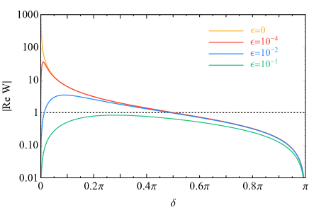
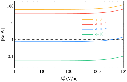
Figure 2: Left: the weak value $\textrm{Re}W$ in Eq. (31) as a function of $\delta$ with $E_{y}^{0}=10$ V/m fixed. Right: the weak value $\textrm{Re}W$ as a function of $E_{y}^{0}$ with $\delta=0.01\pi$ fixed. In both panels, we take $T=10^{-3}$ sec, $E_{x}^{0}=10^{7}$ V/m, and $d_{\rm n}=10^{-26}\,e$ cm, and vary $\epsilon=0,\,10^{-4},\,10^{-2}$, and $10^{-1}$. The black dotted line corresponds to $|\textrm{Re}W|=1$, which is the eigenvalue of $\hat{\sigma}_{x}$.

As we will show in the next section, choosing suitable input parameters such like $\epsilon,\,\delta,\,T,$ and $E_{y}^{0}/E_{x}^{0}$, the weak value $\textrm{Re}W$ can be significantly amplified, and it is just the weak value amplification.

Although we analytically obtain the expectation value of the deviation of the neutron position from $x=0$ as $\Delta_{x}^{W}$ up to corrections of $\mathcal{O}\left((g_{\mu}\alpha T)^{2}\right)$, we will also give the full-order result in Appendix B. In the leading-order analysis in Eq. (42), the EDM signal induced by $\chi$ can be enhanced by large value of $\alpha Td^{2}$. We find, however, that the EDM signal is not amplified by the large value of $\alpha Td^{2}$ in the full-order analysis, because an additional damping factor appears as we will discuss in the next section.

It is important to distinguish the neutron EDM signal from the background shift. Since the background effect depends on many parameters and is complicated in our setup, we evaluate it numerically in the next section.

Before closing this section, let us comment on a special setup in which $\hat{\bf E}=0$ with pre- and post-selections. In such a case, $\Delta_{x}^{W}=(p_{x0}/m_{\rm n})T$ is predicted. Therefore, the first term Eq. (42) can be subtracted by using data of a setup where the external electric field is turned off.

IV Numerical results

In this section, we show numerical results with varying many input parameters. Here and hereafter, we assume the following neutron beam velocity:

$$v_{\rm n}=10^{3}\,{\rm m}/{\rm sec}\,,\quad n_{p_{x0}}=n_{p_{y0}}=0\,,\quad n_{p_{z0}}=1\,,$$ (51)

and the neutron beam size

$$d=0.1\,{\rm m}\,,$$ (52)

where $v_{\rm n}$ and $d$ are reasonable values in the J-PARC neutron beam experiment Mishima et al. (2009); Nakajima et al. (2017), while ideal values of $n_{p_{x0,y0}}$ are taken.

First, we show the weak value $\textrm{Re}W$ in Eq. (31) in Fig. 2. In both panel, the black dotted lines represent $\textrm{Re}W=\pm 1$, which corresponds to the eigenvalues of $\hat{\sigma}_{x}$. Hence, the weak value gives amplification of the signals for the regions with $|\textrm{Re}W|>1$. In the left panel, we investigate $\delta$ and $\epsilon$ dependence, where $T=10^{-3}$ sec, $E_{x}^{0}=10^{7}$ V/m, $E_{y}^{0}=10\,$V/m, and $d_{\rm n}=10^{-26}\,e$ cm are taken.

Here, we classify the weak measurement in the setup. Taking $\delta=\pi$ ($\alpha=0$ in Ref. Aharonov et al. (1988)) corresponds to an ordinary indirect measurement, where the final beam shift is given by the eigenvalue of the spin operator of the EDM direction $\langle\psi|\hat{\sigma}_{x}|\psi\rangle$, in addition to the classical motion [the first term in Eq. (42)]. In this setup, $|\psi\rangle$ is set as $|+_{y}\rangle$ omitting the impurity $\epsilon$, so that a zero eigenvalue is obtained as $\langle+_{y}|\hat{\sigma}_{x}|+_{y}\rangle=0$, which implies that the beam shift occurs only by the classical motion. As you can see in the left panel of Fig. 2, the weak value $W$ is significantly suppressed around $\delta=\pi$. Also, one can consider a different setup: $\delta=\pi$ with $|\psi\rangle=|+_{x}\rangle$. In this case, the beam shift is given by $\langle+_{x}|\hat{\sigma}_{x}|+_{x}\rangle=1$ term in addition to the classical motion. The black dotted line in Fig. 2 shows this latter setup.

It is shown that the weak value amplification, $|{\rm Re}W|>1$, occurs when $\epsilon\lesssim 10^{-2}$, and the amplification is maximized for small $\delta$ regions. As you can see, two orders of magnitude amplification is possible by small $\epsilon$ and $\delta$. In the right panel, $E_{y}^{0}$ dependence of the weak value is investigated, where $\delta=0.01\pi$ is fixed. It is found that $E_{y}^{0}$ dependence is negligible. Note that we also observed that the weak value is insensitive to $T$, $E_{x}^{0}$, and $d_{\rm n}$ for $|g_{\mu}E_{x}^{0}T|\ll 1$ region [see Eq. (47)]. Above results show that the weak value amplification can be controlled by only the polarization angle $\delta$ and the selection impurity $\epsilon$ in the pre- and post-selections.

Here, we comment about a weak-measurement approximation, which is evaluation up to the first order of $\chi$. For $d_{\rm n}=10^{-26}~{}e~{}{\rm cm}$, the parameter $\chi$ is $1.49\times 10^{-7}$, and the real part of the weak value ${\rm Re}\,W$ is smaller than $10^{3}$ according to the left panel of Fig. 2. Consequently, our evaluation based on the weak-measurement approximation is valid.

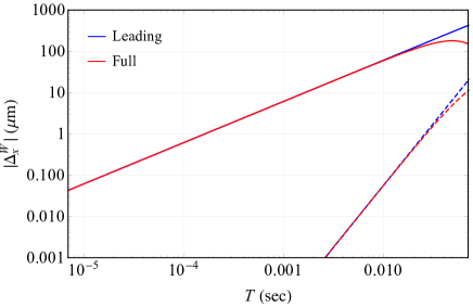
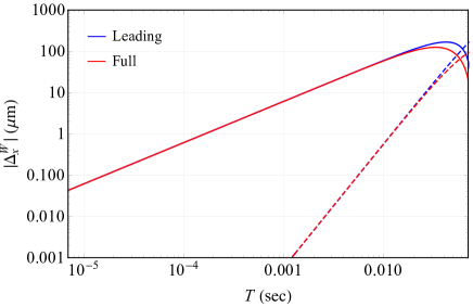
Figure 3: The expected position shift of the center-of-mass of the neutron bunch $\Delta_{x}^{W}$ is shown as a function of $T$. The solid lines stand for the EDM signal parts $\Delta_{x}^{W}(\textrm{EDM})$ with $d_{\rm n}=10^{-25}\,e$ cm, while the dashed lines are for the background effects $\Delta_{x}^{W}(\textrm{BG})$. The blue and red lines represent the leading-order calculations and the full-order ones. In the left and right panels, we take $E_{x}^{0}=10^{6}$ and $10^{7}$ V/m, respectively. In both panels, $\epsilon=0$, $\delta=10^{-3}$, $E_{y}^{0}=10$ V/m, and $\alpha=10^{8}$ V/m² are taken.

Next, we compare the leading-order approximation with respect to $g_{\mu}\alpha T$, which is shown in the previous section, with the full-order analysis. Since equations for the full-order analysis are lengthy, we put them on Appendix B. From the second term of Eq. (42), the expected position shift of the center-of-mass of the neutron bunch is nearly proportional to $\alpha Td^{2}$ within the leading-order approximation. Thus, it is expected that one can amplify the EDM signal by adopting a large value of $\alpha Td^{2}$. This fact is, however, incorrect in the full-order analysis. As shown in Appendix B, the full-order results include a damping factor $\exp\left\{-(g_{\mu}\alpha T)^{2}[d^{2}+(T/2m_{\rm n})^{2}/4d^{2}]/2\right\}$ with respect to $\alpha Td^{2}$ appeared in Eqs. (78) and (79). Since this damping factor becomes significant for a region of

$$g_{\mu}\alpha Td>1\,,$$ (53)

the EDM signal cannot be amplified by the large value of $\alpha Td^{2}$. This factor comes from a Gaussian integral,

$$\int dx\frac{1}{\sqrt{2\pi d^{2}}}e^{i(g_{\mu}\alpha T)x}e^{-\frac{x^{2}}{2d^{2}}}=e^{-\frac{1}{2}(g_{\mu}\alpha T)^{2}d^{2}}\,,$$ (54)

and makes the transition probability in Eq. (37) finite even when $\delta\to 0$ and the ideal experimental setup limit are taken: $E^{0}_{y}/E_{x}^{0}\to 0$, $n_{p_{x0,y0}}\to 0$, and $\epsilon\to 0$.

In Fig. 3, we show the expected position shift of the center-of-mass of the neutron bunch $\Delta_{x}^{W}$ as a function of $T$. In both panels, the solid lines stand for the EDM signal parts $\Delta_{x}^{W}(\textrm{EDM})$, which are proportional to $\chi$, with $d_{\rm n}=10^{-25}\,e$ cm. On the other hand, the dashed lines are for the background effects $\Delta_{x}^{W}(\textrm{BG})$, which are $\chi$ independent. The blue and red lines correspond to the leading-order calculations and the full-order ones, respectively. We take $\epsilon=0$, $\delta=10^{-3}$, $E_{y}^{0}=10$ V/m, $\alpha=10^{8}$ V/m², and $E_{x}^{0}=10^{6}$ ($10^{7}$) V/m for the left (right) panel.

It is shown that, the leading- and the full-order calculations are well consistent with each other in small $T$ regions. On the other hand, $\Delta_{x}^{W}$ is significantly suppressed for large $T$ regions. This figures also show that the background effects in small $T$ region are smaller than the EDM signal contributions by several orders of magnitude, which has been shown analytically in the previous section. In order to suppress the background effects, we adopt $T=0.01\,{\rm sec}$ in following estimations. We also find that the EDM signal contribution is insensitive to $E_{x}^{0}$, while the background effect is sensitive. Note that the background effect is also scaled by $E_{y}^{0}$ [see Eq. (49)].

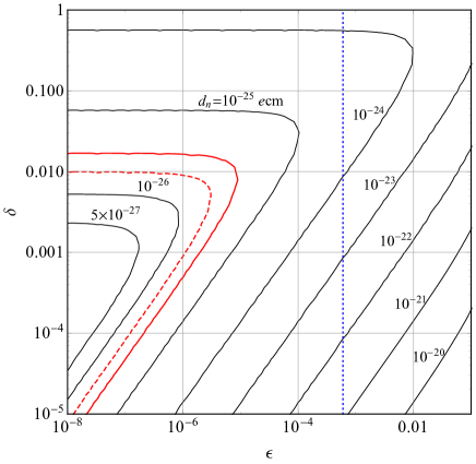
Figure 4: The potential sensitivity to the neutron EDM as functions of the selection impurity $\epsilon$ and the polarization angle $\delta$ in the pre- and post-selections. Here, we take $T=0.01$ sec, $E_{x}^{0}=10^{7}$ V/m, $E_{y}^{0}=10$ V/m, and $\alpha=10^{8}$ V/m².

Finally, we show a potential sensitivity of the weak measurement that can probe the neutron EDM signal. In this setup, the neutron EDM can be probed by precise measurement of $\Delta_{x}^{W}$. In current technology, it is possible to measure the neutron position by several methods with spatial resolutions of $100\,{\rm nm}$ Naganawa et al. (2018), $1\,\mu{\rm m}$ Jenke et al. (2013), $2\,\mu{\rm m}$ Hussey et al. (2017), $5\,\mu{\rm m}$ Matsubayashi et al. (2010); Trtik and Lehmann (2016), $22\,\mu{\rm m}$, Shishido et al. (2018), and $50\,\mu{\rm m}$ Kuroda (1989). These spatial resolutions determine the potential sensitivity to the neutron EDM signal. The detector schemes of Refs. Matsubayashi et al. (2010); Trtik and Lehmann (2016); Shishido et al. (2018); Kuroda (1989) are examined for the neutron beam, and a thermal neutron is examined in Ref. Hussey et al. (2017). On the other hand, the ones of Refs. Jenke et al. (2013); Naganawa et al. (2018) are examined for the UCN, but they can also be utilized for cold neutron (neutron beam) with small detection efficiency Mishima . Recently, the detector scheme of Ref. Naganawa et al. (2018) has been improved Mishima , and the detection efficiency becomes $\mathcal{O}(1\%)$ with spatial resolution of $1\text{--}2\,\mu{\rm m}$ for the cold neutron. Although the emitted neutron beam size is significantly larger than the spatial resolution of the detector, it would not raise a matter. Rather, the spatial resolution should be compared with the statistical uncertainty of the beam size, which will be discussed in the end of this section.

By requiring a condition $|\Delta_{x}^{W}|>1\,\mu{\rm m}$ as a reference value, we show the sensitivity to the neutron EDM in Fig. 4, where $\Delta_{x}^{W}$ includes both the EDM signal and the background shift, and the full-order formalism is used. Here, notice that the information necessary for this analysis is only a time-averaged shift of the center-of-mass of the neutrons passing the post-selection. The sensitivity is shown as a contour on the $\epsilon$–$\delta$ plane, here we take $T=0.01$ sec, $E_{x}^{0}=10^{7}$ V/m, $E_{y}^{0}=10$ V/m, and $\alpha=10^{8}$ V/m². Based on parameters in Refs. Piegsa (2013); Dress et al. (1977b) and discussions with an experimentalist at the J-PARC Mishima , these parameters are chosen. In the Fig. 4, the red (dashed) line corresponds to the current (improved) neutron EDM bound in Eq. (1) [Eq. (2)], and the larger $d_{\rm n}$ region is excluded. Moreover, we find the background effect is negligible on this plane.

We show that the impurity effect changes the sensitivity drastically, and find that the neutron EDM signal can be probed for a very small impurity region, $\epsilon<10^{-5}$. It is two orders of magnitude smaller than the current technology, e.g., $\epsilon=(6\pm 1_{\rm stat.}\pm 3_{\rm sys.})\times 10^{-4}$ Yoshioka et al. (2011), which is shown as the vertical blue dotted line in Fig. 4: the setup with $\epsilon=6\times 10^{-4}$ and $\delta=0.1$ $=5.7^{\circ}$ could probe a region $d_{\rm n}>3\times 10^{-25}~{}e\,{\rm cm}$.

We comment on contributions from nonzero $n_{p_{x0}}$ and $n_{p_{y0}}$ values. We find that if $n_{p_{x0,y0}}$ are smaller than $10^{-5}$, these effects do not appear in above numerical evaluations. We also find that the effect of $n_{p_{y0}}$ is more significant than $n_{p_{x0}}$: $\mathcal{O}(1)$ contributions are produced for $n_{p_{y0}}\sim 10^{-4}$ region.

We also comment on a statistical condition for measuring non-zero $\Delta_{x}^{W}$, where we compare the spatial resolution of the detector with the statistical uncertainty of the neutron beam. In such an experiment, one has to reject a null hypothesis of the neutron beam following the Gaussian distribution with the average position $0$ and the variance $d^{2}$. If one measures the time-averaged shift of the center-of-mass of the neutrons by $\mathcal{N}$ neutrons, the statistical condition for measuring non-zero $\Delta_{x}^{W}$ at $n\sigma$ level is expressed as $\Delta_{x}^{W}>n\cdot d/\sqrt{\mathcal{N}}$. If one considers a case that a resolution of $1\,\mu$m for $\Delta_{x}^{W}$ and $d=0.1\,{\rm m}$, the condition is $\mathcal{N}>10^{10}n^{2}$. In this setup, the number of neutrons $\mathcal{N}$ is

$$\mathcal{N}\simeq\mathcal{N}_{0}\cdot 2\epsilon\cdot\varepsilon_{\rm eff}\,,$$ (55)

where $\mathcal{N}_{0}$ represents the number of emitted neutrons, $2\epsilon$ is the neutron passing probability at the post-selection in Eq. (41), and $\varepsilon_{\rm eff}$ is the detection efficiency at the detector. Then, the statistical condition is

$$\mathcal{N}_{0}>\frac{10^{10}n^{2}}{2\epsilon\varepsilon_{\rm eff}}\,.$$ (56)

Since the $\mathcal{O}(10^{9})$ neutrons can be generated per second in the experiment Nakajima et al. (2017), a required time is $t>5n^{2}/(\epsilon\varepsilon_{\rm eff})$ sec. Even if the detection efficiency for the neutron beam is $\mathcal{O}(1\%)$ Jenke et al. (2013); Mishima , the statistical condition for $n=2$ is satisfied by $\mathcal{O}(2000/\epsilon)$ seconds neutron beam.

V Conclusions

In this paper, we proposed a novel approach in a search for the neutron EDM by applying the weak measurement, which is independent from the Ramsey method. Although the relativistic ${\bf E}\times{\bf v}$ effect provides a severe systematic uncertainty in the neutron EDM experiment in which the neutron beam is used, we find such a contribution is numerically irrelevant in the weak measurement. This is quite unexpected result, and we believe that this fact would provide a new virtue of the weak measurement.

To investigate a potential sensitivity to the neutron EDM search, we included the effect from the selection impurities in the pre- and post-selections. Our study showed that the size of the impurity crucially determines the sensitivity.

We found that the weak measurement can reach up to $d_{\rm n}>3\times 10^{-25}~{}e\,{\rm cm}$ within the current technology. This is one order of magnitude less sensitive that the current neutron EDM bound, where the UCNs based on the Ramsey method are used.

In addition, our approach could provide a new possibility to measure the weak value of the neutron spin polarization from the background effect. This fact makes our study fascinating in the point of view of the quantum mechanics.

The detailed study about the Fisher information based on Ref. Harris et al. (2017) would be one of future directions of this study, where one can explore whether the weak-value amplification in the neutron EDM measurement outperforms the conventional Ramsey method one. Also, the perturbative effects from the Gaussian beam profile Clark et al. (2015) could give additional systematic error in the weak measurement Turek et al. (2015).

Although the small impurity, $\epsilon<10^{-5}$, for probing the neutron EDM is difficult at the present time, we hope several improvements on the experimental technology, e.g., the sensitivity can be amplified by $\alpha$ and the resolution of $\Delta_{x}^{W}$ measurement, and anticipate that this kind of experiment will be performed in future.

Appendix A External electric field with gradient

In this appendix, we consider a general setup of the external electric field with spatial gradients. Let us consider an external electric field with gradients $\partial\hat{\bf E}/{\partial x}=(\alpha_{x},\,\alpha_{y},\,0)$:

$$\hat{\bf E}(x)=\left(E_{x}^{0}+\alpha_{x}x,\,E_{y}^{0}+\alpha_{y}x,\,0\right)\,,$$ (57)

where $E_{x,y}^{0}$ and $\alpha_{x,y}$ are constants. Note that the setup is insensitive to $E_{z}$ component and its relativistic effect.

When one considers a rotation of the coordinate that all spatial dependence go to single electric filed component, the following $\hat{\bf E}$ with a coordinate ${\bf x}^{\prime}$ are obtained:

$$\hat{\bf E}^{\prime}(x^{\prime},y^{\prime})^{T} =R\hat{\bf E}^{T}=\frac{1}{\sqrt{\alpha_{x}^{2}+\alpha_{y}^{2}}}\begin{pmatrix}\alpha_{x}E_{x}^{0}+\alpha_{y}E_{y}^{0}+(\alpha_{x}^{2}+\alpha_{y}^{2})x\\ -\alpha_{y}E_{x}^{0}+\alpha_{x}E_{y}^{0}\\ 0\end{pmatrix}$$ (58)

$$=\begin{pmatrix}\frac{1}{\sqrt{\alpha_{x}^{2}+\alpha_{y}^{2}}}(\alpha_{x}E_{x}^{0}+\alpha_{y}E_{y}^{0})+\alpha_{x}x^{\prime}-\alpha_{y}y^{\prime}\\ \frac{1}{\sqrt{\alpha_{x}^{2}+\alpha_{y}^{2}}}(-\alpha_{y}E_{x}^{0}+\alpha_{x}E_{y}^{0})\\ 0\end{pmatrix}\,,$$ (59)

and

$${\bf x}^{\prime}\equiv\begin{pmatrix}x^{\prime}\\ y^{\prime}\\ z^{\prime}\end{pmatrix}=R{\bf x}=\frac{1}{\sqrt{\alpha_{x}^{2}+\alpha_{y}^{2}}}\begin{pmatrix}\alpha_{x}x+\alpha_{y}y\\ -\alpha_{y}x+\alpha_{x}y\\ z\end{pmatrix}\,,$$ (60)

where the rotation matrix $R$ is

$$R=\begin{pmatrix}\cos\theta&\sin\theta&0\\ -\sin\theta&\cos\theta&0\\ 0&0&1\end{pmatrix}\,,~{}~{}{\rm with}~{}~{}\cos\theta=\frac{\alpha_{x}}{\sqrt{\alpha_{x}^{2}+\alpha_{y}^{2}}}\,.$$ (61)

The spatial dependence of $y^{\prime}$ in $\hat{\bf E}^{\prime}(x^{\prime},y^{\prime})$ would provide us with a spatial displacement of the neutron along $y^{\prime}$ axis. In order to obtain the experimental setup in Eq. (10), $\alpha_{y}\ll\alpha_{x}$ are thus required.

Appendix B Full-order calculation for $\Delta_{x}^{W}$

In this appendix, we give building blocks of the full-order calculation for $\Delta_{x}^{W}$ with respect to $g_{\mu}\alpha T$. The expected position shift of the center-of-mass of the neutron bunch is defined as [see Eqs. (37), (38), and (42) for the leading-order analysis]:

$$\Delta_{x}^{W}=\frac{{\rm Tr}\left[\left(\hat{x}+\frac{T}{2m_{\rm n}}\hat{p}_{x}\right)\hat{\rho}^{\rm total}_{\rm fin}\right]}{{\rm Tr}\left[\hat{\rho}^{\rm total}_{\rm fin}\right]}\,,$$ (62)

with

$${\rm Tr}\left[\hat{\rho}^{\rm total}_{\rm fin}\right] ={\langle G_{p_{x0}}|{\rm Tr}_{S}\left[\hat{\rho}^{S}_{\rm fin}e^{-iT\hat{H}}\hat{\rho}^{S}_{\rm ini}e^{iT\hat{H}}\right]|G_{p_{x0}}\rangle}\,,$$ (63)

$${\rm Tr}\left[\left(\hat{x}+\frac{T}{2m_{\rm n}}\hat{p}_{x}\right)\hat{\rho}^{\rm total}_{\rm fin}\right] ={\langle G_{p_{x0}}|\left(\hat{x}+\frac{T}{2m_{\rm n}}\hat{p}_{x}\right){\rm Tr}_{S}\left[\hat{\rho}^{S}_{\rm fin}e^{-iT\hat{H}}\hat{\rho}^{S}_{\rm ini}e^{iT\hat{H}}\right]|G_{p_{x0}}\rangle}\,.$$ (64)

In the full-order analysis, we discard only $\mathcal{O}(\chi^{2})$ contributions. Using Eqs. (15)–(17) for the time evolution operator, ${\rm Tr}_{S}[\hat{\rho}^{S}_{\rm fin}e^{-iT\hat{H}}\hat{\rho}^{S}_{\rm ini}e^{iT\hat{H}}]$ is expanded as

$${\rm Tr}_{S}\left[\hat{\rho}^{S}_{\rm fin}e^{-iT\hat{H}}\hat{\rho}^{S}_{\rm ini}e^{iT\hat{H}}\right]= e^{-iT\frac{\hat{p}^{2}_{x}}{2m_{\rm n}}}\biggl{\{}-\frac{1}{2\hat{E}_{x}^{2}}\bigg{[}\hat{E}_{x}^{2}(-1+(1-2\epsilon)^{2}\cos(\delta))\cos^{2}(\hat{E}_{x}g_{\mu}T)-(E^{0}_{y}n_{p_{x0}}-\hat{E}_{x}n_{p_{y0}})^{2}\sin^{2}(\hat{E}_{x}gT)$$

$$-(\hat{E}_{x}^{2}+(E^{0}_{y})^{2})n_{p_{z0}}^{2}\sin^{2}(\hat{E}_{x}g_{\mu}T)-(1-2\epsilon)^{2}(E^{0}_{y}n_{p_{x0}}-\hat{E}_{x}n_{p_{y0}})^{2}\cos(\delta)\sin^{2}(\hat{E}_{x}g_{\mu}T)$$

$$-(1-2\epsilon)^{2}(-\hat{E}_{x}+E^{0}_{y})(\hat{E}_{x}+E^{0}_{y})n_{p_{z0}}^{2}\cos(\delta)\sin^{2}(\hat{E}_{x}g_{\mu}T)$$

$$-2(1-2\epsilon)^{2}\hat{E}_{x}(E^{0}_{y}n_{p_{x0}}-\hat{E}_{x}n_{p_{y0}})n_{p_{z0}}\sin(\delta)\sin^{2}(\hat{E}_{x}g_{\mu}T)+(1-2\epsilon)^{2}\hat{E}_{x}E^{0}_{y}n_{p_{z0}}\sin(\delta)\sin(2\hat{E}_{x}g_{\mu}T)\bigg{]}$$

$$-\chi\frac{1}{2\hat{E}_{x}^{2}}\bigg{[}-2\hat{E}_{x}E^{0}_{y}n_{p_{z0}}\sin^{2}(\hat{E}_{x}g_{\mu}T)-2(1-2\epsilon)^{2}\hat{E}_{x}E^{0}_{y}n_{p_{z0}}\cos(\delta)\sin^{2}(\hat{E}_{x}g_{\mu}T)$$

$$+(1-2\epsilon)^{2}\hat{E}_{x}^{2}\sin(\delta)\sin(2\hat{E}_{x}g_{\mu}T)\bigg{]}\biggr{\}}e^{+iT\frac{\hat{p}^{2}_{x}}{2m_{\rm n}}}+\mathcal{O}(\chi^{2})\,,$$ (65)

where $\hat{E}_{x}$ is defined as $\hat{E}_{x}=E_{x}^{0}+\alpha\left(\hat{x}+T\hat{p}_{x}/2m_{\rm n}\right)$. To calculate Eqs. (63) and (64), the following building blocks are needed:

$${\langle G_{p_{x0}}|e^{-iT\frac{\hat{p}_{x}^{2}}{2m_{\rm n}}}\cos^{2}\left(\hat{E}_{x}g_{\mu}T\right)e^{+iT\frac{\hat{p}_{x}^{2}}{2m_{\rm n}}}|G_{p_{x0}}\rangle}=\frac{1}{4}\left[f_{1}(2g_{\mu})+f_{1}(-2g_{\mu})+2\right]\,,$$ (66)

$${\langle G_{p_{x0}}|e^{-iT\frac{\hat{p}_{x}^{2}}{2m_{\rm n}}}\sin^{2}\left(\hat{E}_{x}g_{\mu}T\right)e^{+iT\frac{\hat{p}_{x}^{2}}{2m_{\rm n}}}|G_{p_{x0}}\rangle}=-\frac{1}{4}\left[f_{1}(2g_{\mu})+f_{1}(-2g_{\mu})-2\right]\,,$$ (67)

$${\langle G_{p_{x0}}|e^{-iT\frac{\hat{p}_{x}^{2}}{2m_{\rm n}}}\frac{1}{\hat{E}_{x}^{2}}\sin^{2}\left(\hat{E}_{x}g_{\mu}T\right)e^{+iT\frac{\hat{p}_{x}^{2}}{2m_{\rm n}}}|G_{p_{x0}}\rangle}=T^{2}\int_{0}^{g_{\mu}}dg_{1}\int_{0}^{g_{1}}dg_{2}\left[f_{1}(2g_{2})+f_{1}(-2g_{2})\right]\,,$$ (68)

$${\langle G_{p_{x0}}|e^{-iT\frac{\hat{p}_{x}^{2}}{2m_{\rm n}}}\frac{1}{\hat{E}_{x}}\sin^{2}\left(\hat{E}_{x}g_{\mu}T\right)e^{+iT\frac{\hat{p}_{x}^{2}}{2m_{\rm n}}}|G_{p_{x0}}\rangle}=\frac{T}{2i}\int_{0}^{g_{\mu}}dg_{1}\left[f_{1}(2g_{1})-f_{1}(-2g_{1})\right]\,,$$ (69)

$${\langle G_{p_{x0}}|e^{-iT\frac{\hat{p}_{x}^{2}}{2m_{\rm n}}}\sin\left(2\hat{E}_{x}g_{\mu}T\right)e^{+iT\frac{\hat{p}_{x}^{2}}{2m_{\rm n}}}|G_{p_{x0}}\rangle}=\frac{1}{2i}\left[f_{1}(2g_{\mu})-f_{1}(-2g_{\mu})\right]\,,$$ (70)

$${\langle G_{p_{x0}}|e^{-iT\frac{\hat{p}_{x}^{2}}{2m_{\rm n}}}\frac{1}{\hat{E}_{x}}\sin\left(2\hat{E}_{x}g_{\mu}T\right)e^{+iT\frac{\hat{p}_{x}^{2}}{2m_{\rm n}}}|G_{p_{x0}}\rangle}=T\int_{0}^{g_{\mu}}dg_{1}\left[f_{1}(2g_{1})+f_{1}(-2g_{1})\right]\,,$$ (71)

$${\langle G_{p_{x0}}|\left(\hat{x}+\frac{T}{2m_{\rm n}}\hat{p}_{x}\right)e^{-iT\frac{\hat{p}_{x}^{2}}{2m_{\rm n}}}\cos^{2}\left(\hat{E}_{x}g_{\mu}T\right)e^{+iT\frac{\hat{p}_{x}^{2}}{2m_{\rm n}}}|G_{p_{x0}}\rangle}=\frac{1}{4}\left[f_{2}(2g_{\mu})+f_{2}(-2g_{\mu})+\frac{T}{2m_{\rm n}}p_{x0}\right]\,,$$ (72)

$${\langle G_{p_{x0}}|\left(\hat{x}+\frac{T}{2m_{\rm n}}\hat{p}_{x}\right)e^{-iT\frac{\hat{p}_{x}^{2}}{2m_{\rm n}}}\sin^{2}\left(\hat{E}_{x}g_{\mu}T\right)e^{+iT\frac{\hat{p}_{x}^{2}}{2m_{\rm n}}}|G_{p_{x0}}\rangle}=-\frac{1}{4}\left[f_{2}(2g_{\mu})+f_{2}(-2g_{\mu})-\frac{T}{2m_{\rm n}}p_{x0}\right]\,,$$ (73)

$${\langle G_{p_{x0}}|\left(\hat{x}+\frac{T}{2m_{\rm n}}\hat{p}_{x}\right)e^{-iT\frac{\hat{p}_{x}^{2}}{2m_{\rm n}}}\frac{1}{\hat{E}_{x}^{2}}\sin^{2}\left(\hat{E}_{x}g_{\mu}T\right)e^{+iT\frac{\hat{p}_{x}^{2}}{2m_{\rm n}}}|G_{p_{x0}}\rangle}=T^{2}\int_{0}^{g_{\mu}}dg_{1}\int_{0}^{g_{1}}dg_{2}\left[f_{2}(2g_{2})+f_{2}(-2g_{2})\right]\,,$$ (74)

$${\langle G_{p_{x0}}|\left(\hat{x}+\frac{T}{2m_{\rm n}}\hat{p}_{x}\right)e^{-iT\frac{\hat{p}_{x}^{2}}{2m_{\rm n}}}\frac{1}{\hat{E}_{x}}\sin^{2}\left(\hat{E}_{x}g_{\mu}T\right)e^{+iT\frac{\hat{p}_{x}^{2}}{2m_{\rm n}}}|G_{p_{x0}}\rangle}=\frac{T}{2i}\int_{0}^{g_{\mu}}dg_{1}\left[f_{2}(2g_{1})-f_{2}(-2g_{1})\right]\,,$$ (75)

$${\langle G_{p_{x0}}|\left(\hat{x}+\frac{T}{2m_{\rm n}}\hat{p}_{x}\right)e^{-iT\frac{\hat{p}_{x}^{2}}{2m_{\rm n}}}\sin\left(2\hat{E}_{x}g_{\mu}T\right)e^{+iT\frac{\hat{p}_{x}^{2}}{2m_{\rm n}}}|G_{p_{x0}}\rangle}=\frac{1}{2i}\left[f_{2}(2g_{\mu})-f_{2}(-2g_{\mu})\right]\,,$$ (76)

$${\langle G_{p_{x0}}|\left(\hat{x}+\frac{T}{2m_{\rm n}}\hat{p}_{x}\right)e^{-iT\frac{\hat{p}_{x}^{2}}{2m_{\rm n}}}\frac{1}{\hat{E}_{x}}\sin\left(2\hat{E}_{x}g_{\mu}T\right)e^{+iT\frac{\hat{p}_{x}^{2}}{2m_{\rm n}}}|G_{p_{x0}}\rangle}=T\int_{0}^{g_{\mu}}dg_{1}\left[f_{2}(2g1)+f_{2}(-2g_{1})\right]\,,$$ (77)

with

$$f_{1}(g_{\mu})\equiv{\langle G_{p_{x0}}|e^{-iT\frac{\hat{p}_{x}^{2}}{2m_{\rm n}}}e^{i\hat{E}_{x}g_{\mu}T}e^{+iT\frac{\hat{p}_{x}^{2}}{2m_{\rm n}}}|G_{p_{x0}}\rangle}$$

$$\quad\quad~{}~{}={e^{i\left(g_{\mu}E_{x}^{0}T-g_{\mu}\alpha T\frac{T}{2m_{\rm n}}p_{x0}\right)}e^{-\frac{(g_{\mu}\alpha T)^{2}}{2}\left[d^{2}+\frac{1}{4d^{2}}\left(\frac{T}{2m_{\rm n}}\right)^{2}\right]}}\,,$$ (78)

$$f_{2}(g_{\mu})\equiv{\langle G_{p_{x0}}|e^{-iT\frac{\hat{p}_{x}^{2}}{2m_{\rm n}}}\left(\hat{x}+\frac{T}{2m_{\rm n}}\hat{p}_{x}\right)e^{i\hat{E}_{x}g_{\mu}T}e^{+iT\frac{\hat{p}_{x}^{2}}{2m_{\rm n}}}|G_{p_{x0}}\rangle}$$

$$\quad\quad~{}~{}={\left\{-\frac{T}{2m_{\rm n}}(p_{x0}+g_{\mu}\alpha T)+ig_{\mu}\alpha T\left[d^{2}+\frac{1}{4d^{2}}\left(\frac{T}{2m_{\rm n}}\right)^{2}\right]\right\}e^{i\left(g_{\mu}E_{x}^{0}T-g_{\mu}\alpha T\frac{T}{2m_{\rm n}}p_{x0}\right)}e^{-\frac{(g_{\mu}\alpha T)^{2}}{2}\left[d^{2}+\frac{1}{4d^{2}}\left(\frac{T}{2m_{\rm n}}\right)^{2}\right]}}\,.$$ (79)

Combining Eqs. (63)–(79), one can numerically calculate the expected position shift of the center-of-mass of the neutron bunch at the full order. See e.g., Refs. Lee and Tsutsui (2014); Kawana and Ueda (2019) for detailed discussions of the damping factors in Eqs. (78) and (79).

References

- Kobayashi and Maskawa (1973) M. Kobayashi and T. Maskawa, “CP Violation in the Renormalizable Theory of Weak Interaction,” Prog. Theor. Phys. 49, 652–657 (1973).
- Ramsey (1982) N. F. Ramsey, “Electric-Dipole Moments of Particles,” Ann. Rev. Nucl. Part. Sci. 32, 211–233 (1982).
- Shabalin (1978) E. P. Shabalin, “Electric Dipole Moment of Quark in a Gauge Theory with Left-Handed Currents,” Sov. J. Nucl. Phys. 28, 75 (1978), [Yad. Fiz.28,151(1978)].
- Khriplovich (1986) I. B. Khriplovich, “Quark Electric Dipole Moment and Induced Term in the Kobayashi-Maskawa Model,” Phys. Lett. B173, 193–196 (1986), [Yad. Fiz.44,1019(1986)].
- Czarnecki and Krause (1997) A. Czarnecki and B. Krause, “Neutron electric dipole moment in the standard model: Valence quark contributions,” Phys. Rev. Lett. 78, 4339–4342 (1997), arXiv:hep-ph/9704355 [hep-ph] .
- Khriplovich and Zhitnitsky (1982) I. B. Khriplovich and A. R. Zhitnitsky, “What Is the Value of the Neutron Electric Dipole Moment in the Kobayashi-Maskawa Model?” Phys. Lett. 109B, 490–492 (1982).
- McKellar et al. (1987) B. H. J. McKellar, S. R. Choudhury, X.-G. He, and S. Pakvasa, “The Neutron Electric Dipole Moment in the Standard m Model,” Phys. Lett. B197, 556–560 (1987).
- Dragos et al. (2021) J. Dragos, T. Luu, A. Shindler, J. de Vries, and A. Yousif, “Confirming the Existence of the strong CP Problem in Lattice QCD with the Gradient Flow,” Phys. Rev. C 103, 015202 (2021), arXiv:1902.03254 [hep-lat] .
- Mannel and Uraltsev (2012) T. Mannel and N. Uraltsev, “Loop-Less Electric Dipole Moment of the Nucleon in the Standard Model,” Phys. Rev. D85, 096002 (2012), arXiv:1202.6270 [hep-ph] .
- Weinberg (1976) S. Weinberg, “Gauge Theory of CP Violation,” Phys. Rev. Lett. 37, 657 (1976).
- Deshpande and Ma (1977) N. G. Deshpande and E. Ma, “Comment on Weinberg’s Gauge Theory of CP Nonconservation,” Phys. Rev. D16, 1583 (1977).
- Weinberg (1989) S. Weinberg, “Larger Higgs Exchange Terms in the Neutron Electric Dipole Moment,” Phys. Rev. Lett. 63, 2333 (1989).
- Barr and Zee (1990) S. M. Barr and A. Zee, “Electric Dipole Moment of the Electron and of the Neutron,” Phys. Rev. Lett. 65, 21–24 (1990), [Erratum: Phys. Rev. Lett.65,2920(1990)].
- Ellis et al. (1982) J. R. Ellis, S. Ferrara, and D. V. Nanopoulos, “CP Violation and Supersymmetry,” Phys. Lett. 114B, 231–234 (1982).
- Buchmuller and Wyler (1983) W. Buchmuller and D. Wyler, “CP Violation and R Invariance in Supersymmetric Models of Strong and Electroweak Interactions,” Proceedings, DESY Workshop on Electroweak Interactions at High Energies: Hamburg, Germany, September 28-30, 1982, Phys. Lett. 121B, 321 (1983), [,277(1982)].
- Polchinski and Wise (1983) J. Polchinski and M. B. Wise, “The Electric Dipole Moment of the Neutron in Low-Energy Supergravity,” Phys. Lett. 125B, 393–398 (1983).
- Dugan et al. (1985) M. Dugan, B. Grinstein, and L. J. Hall, “CP Violation in the Minimal N=1 Supergravity Theory,” Nucl. Phys. B255, 413–438 (1985).
- Arnold et al. (2013) J. M. Arnold, B. Fornal, and M. B. Wise, “Phenomenology of scalar leptoquarks,” Phys. Rev. D88, 035009 (2013), arXiv:1304.6119 [hep-ph] .
- Fuyuto et al. (2019) K. Fuyuto, M. Ramsey-Musolf, and T. Shen, “Electric Dipole Moments from CP-Violating Scalar Leptoquark Interactions,” Phys. Lett. B788, 52–57 (2019), arXiv:1804.01137 [hep-ph] .
- Dekens et al. (2019) W. Dekens, J. de Vries, M. Jung, and K. K. Vos, “The phenomenology of electric dipole moments in models of scalar leptoquarks,” JHEP 01, 069 (2019), arXiv:1809.09114 [hep-ph] .
- Appelquist et al. (2004a) T. Appelquist, M. Piai, and R. Shrock, “Lepton dipole moments in extended technicolor models,” Phys. Lett. B593, 175–180 (2004a), arXiv:hep-ph/0401114 [hep-ph] .
- Appelquist et al. (2004b) T. Appelquist, M. Piai, and R. Shrock, “Quark dipole operators in extended technicolor models,” Phys. Lett. B595, 442–452 (2004b), arXiv:hep-ph/0406032 [hep-ph] .
- Sakharov (1967) A. D. Sakharov, “Violation of CP Invariance, C asymmetry, and baryon asymmetry of the universe,” Pisma Zh. Eksp. Teor. Fiz. 5, 32–35 (1967), [Usp. Fiz. Nauk161,no.5,61(1991)].
- Gavela et al. (1994) M. B. Gavela, P. Hernandez, J. Orloff, and O. Pene, “Standard model CP violation and baryon asymmetry,” Mod. Phys. Lett. A9, 795–810 (1994), arXiv:hep-ph/9312215 [hep-ph] .
- Fuyuto et al. (2016) K. Fuyuto, J. Hisano, and E. Senaha, “Toward verification of electroweak baryogenesis by electric dipole moments,” Phys. Lett. B755, 491–497 (2016), arXiv:1510.04485 [hep-ph] .
- Pendlebury et al. (2015) J. M. Pendlebury et al., “Revised experimental upper limit on the electric dipole moment of the neutron,” Phys. Rev. D92, 092003 (2015), arXiv:1509.04411 [hep-ex] .
- Ramsey (1949) N. F. Ramsey, “A New Molecular Beam Resonance Method,” Phys. Rev. 76, 996 (1949).
- Ramsey (1950) N. F. Ramsey, “A Molecular Beam Resonance Method with Separated Oscillating Fields,” Phys. Rev. 78, 695–699 (1950).
- (29) G. Pignol, “The new measurement of the neutron EDM,” PSI user’s meeting, PSI Villigen, 28 January 2020.
- Abel et al. (2020) C. Abel et al. (nEDM), “Measurement of the permanent electric dipole moment of the neutron,” Phys. Rev. Lett. 124, 081803 (2020), arXiv:2001.11966 [hep-ex] .
- Smith et al. (1957) J. H. Smith, E. M. Purcell, and N. F. Ramsey, “Experimental limit to the electric dipole moment of the neutron,” Phys. Rev. 108, 120–122 (1957).
- Baird et al. (1969) J. K. Baird, P. D. Miller, W. B. Dress, and N. F. Ramsey, “Improved upper limit to the electric dipole moment of the neutron,” Phys. Rev. 179, 1285–1291 (1969).
- Dress et al. (1977a) W. B. Dress, P. D. Miller, J. M. Pendlebury, Paul Perrin, and Norman F. Ramsey, “Search for an Electric Dipole Moment of the Neutron,” Phys. Rev. D15, 9 (1977a).
- Ramsey (1986) N. F. Ramsey, “Neutron magnetic resonance experiments,” Physica BC137, 223 (1986).
- Feynman et al. (1964) R. Feynman, R. Leighton, and M. Sands, “The Feynman’s Lectures on Physics,” (1964), Volume II.
- Altarev et al. (1996) I. S. Altarev et al., “Search for the neutron electric dipole moment,” Phys. Atom. Nucl. 59, 1152–1170 (1996), [Yad. Fiz.59N7,1204(1996)].
- Baker et al. (2006) C. A. Baker et al., “An Improved experimental limit on the electric dipole moment of the neutron,” Phys. Rev. Lett. 97, 131801 (2006), arXiv:hep-ex/0602020 [hep-ex] .
- Ito (2007) T. M. Ito, “Plans for a Neutron EDM Experiment at SNS,” 2nd Meeting of the APS Topical Group on Hadronic Physics (GHP2006) Nashville, Tennesse, October 22-24, 2006, J. Phys. Conf. Ser. 69, 012037 (2007), arXiv:nucl-ex/0702024 [NUCL-EX] .
- van der Grinten et al. (2009) M. G. D. van der Grinten et al. (CryoEDM), “CryoEDM: A cryogenic experiment to measure the neutron electric dipole moment,” Particle physics with slow neutrons. Proceedings, International Workshop, Grenoble, France, May 29-31, 2008, Nucl. Instrum. Meth. A611, 129–132 (2009).
- Serebrov et al. (2009) A. P. Serebrov et al., “Ultracold-neutron infrastructure for the PNPI/ILL neutron EDM experiment,” Nucl. Instrum. Meth. A611, 263–266 (2009).
- Lamoreaux and Golub (2009) S. K. Lamoreaux and R. Golub, “Experimental searches for the neutron electric dipole moment,” J. Phys. G36, 104002 (2009).
- Baker et al. (2011) C. A. Baker et al., “The search for the neutron electric dipole moment at the Paul Scherrer Institute,” Proceedings, 2nd International Workshop on Physics of fundamental Symmetries and Interactions at low energies and the precision frontier (PSI2010): PSI, Villigen, Switzerland, October 11-14, 2010, Phys. Procedia 17, 159–167 (2011).
- Masuda et al. (2012) Y. Masuda et al., “Neutron electric dipole moment measurement with a buffer gas comagnetometer,” Phys. Lett. A376, 1347 (2012).
- Altarev et al. (2012) I. Altarev et al., “A next generation measurement of the electric dipole moment of the neutron at the FRM II,” 5th International Workshop on From Parity Violation to Hadronic Structure and More (PAVI11) Rome, Italy, September 5-9, 2011, Nuovo Cim. C035N04, 122–127 (2012).
- Piegsa (2013) F. M. Piegsa, “New Concept for a Neutron Electric Dipole Moment Search using a Pulsed Beam,” Phys. Rev. C88, 045502 (2013), arXiv:1309.1959 [physics.ins-det] .
- Fedorov et al. (2005) V. V. Fedorov, E. G. Lapin, E. Lelievre-Berna, V. V. Nesvizhevsky, A. K. Petukhov, S. Y. Semenikhin, T. Soldner, F. Tasset, and V. V. Voronin, “The Laue diffraction method to search for a neutron EDM. Experimental test of the sensitivity,” Nucl. Instrum. Meth. B 227, 11–15 (2005).
- Fedorov et al. (2008) V. V. Fedorov, E. G. Lapin, S. Y. Semenikhin, V. V. Voronin, E. Lelievre-Berna, V. Nesvizhevsky, A. Petoukhov, T. Soldner, and F. Tasset, “First observation of the neutron spin rotation for Laue diffraction in a deformed noncentrosymmetric crystal,” Int. J. Mod. Phys. A 23, 1435–1445 (2008).
- Fedorov et al. (2009a) V. V. Fedorov et al., “Measurement of the neutron electric dipole moment by crystal diffraction,” Nucl. Instrum. Meth. A 611, 124–128 (2009a), arXiv:0907.1153 [nucl-ex] .
- Fedorov et al. (2009b) V. V. Fedorov et al., “Perspectives for nEDM search by crystal diffraction. Test experiment and results,” Nucl. Phys. A 827, 538c–540c (2009b).
- Fedorov et al. (2011) V. V. Fedorov et al., “Measurement of the neutron electric dipole moment via spin rotation in a non-centrosymmetric crystal,” Phys. Lett. B 694, 22–25 (2011), arXiv:1009.0153 [hep-ex] .
- Aharonov et al. (1964) Y. Aharonov, P. G. Bergmann, and J. L. Lebowitz, “Time symmetry in the quantum process of measurement,” Phys. Rev. 134, B1410–B1416 (1964).
- Aharonov et al. (1988) Y. Aharonov, D. Z. Albert, and L. Vaidman, “How the result of a measurement of a component of the spin of a spin-1/2 particle can turn out to be 100,” Phys. Rev. Lett. 60, 1351–1354 (1988).
- Lee and Tsutsui (2014) J. Lee and I. Tsutsui, “Merit of amplification by weak measurement in view of measurement uncertainty,” Quantum Studies: Mathematics and Foundations 1, 65–78 (2014).
- Sponar et al. (2015) S. Sponar, T. Denkmayr, H. Geppert, H. Lemmel, A. Matzkin, and Y. Hasegawa, “Weak values obtained in matter-wave interferometry,” Phys. Rev. A92, 062121 (2015), arXiv:1404.2125 [quant-ph] .
- Ritchie et al. (1991) N. W. M. Ritchie, J. G. Story, and Randall G. Hulet, “Realization of a measurement of a “weak value”,” Phys. Rev. Lett. 66, 1107–1110 (1991).
- Pryde et al. (2005) G. J. Pryde, J. L. O’Brien, A. G. White, T. C. Ralph, and H. M. Wiseman, “Measurement of quantum weak values of photon polarization,” Phys. Rev. Lett. 94, 220405 (2005).
- Aharonov et al. (2010) Y. Aharonov, S. Popescu, and J. Tollaksen, “A time-symmetric formulation of quantum mechanics,” Physics Today 63, 27–32 (2010).
- Kofman et al. (2012) A. G. Kofman, S. Ashhab, and F. Nori, “Nonperturbative theory of weak pre- and post-selected measurements,” Phys. Rep. 520, 43–133 (2012), arXiv:1109.6315 [quant-ph] .
- Aharonov and Vaidman (1991) Y. Aharonov and L. Vaidman, “Complete description of a quantum system at a given time,” Journal of Physics A: Mathematical and General 24, 2315–2328 (1991).
- Yokota et al. (2009) K. Yokota, T. Yamamoto, M. Koashi, and N. Imoto, “Direct observation of hardy’s paradox by joint weak measurement with an entangled photon pair,” New Journal of Physics 11, 033011 (2009).
- Hosten and Kwiat (2008) O. Hosten and P. Kwiat, “Observation of the spin hall effect of light via weak measurements,” Science 319, 787–790 (2008).
- Dixon et al. (2009) P. B. Dixon, D. J. Starling, A. N. Jordan, and J. C. Howell, “Ultrasensitive beam deflection measurement via interferometric weak value amplification,” Phys. Rev. Lett. 102, 173601 (2009), arXiv:0906.4828 [quant-ph] .
- Duck et al. (1989) I. M. Duck, P. M. Stevenson, and E. C. G. Sudarshan, “The Sense in Which a “Weak Measurement” of a Spin Particle’s Spin Component Yields a Value ,” Phys. Rev. D 40, 2112–2117 (1989).
- Vaidman (2014) L. Vaidman, “Comment on “How the result of a single coin toss can turn out to be 100 heads”,” (2014), arXiv:1409.5386 [quant-ph] .
- Dressel (2015) J. Dressel, “Weak values as interference phenomena,” Phys. Rev. A 91, 032116 (2015), arXiv:1410.0943 [quant-ph] .
- Qin et al. (2016) L. Qin, W. Feng, and X.-Q. Li, “Simple understanding of quantum weak values,” Scientific Reports 6, 20286 (2016), arXiv:1505.00595 [quant-ph] .
- Pospelov and Ritz (2005) M. Pospelov and A. Ritz, “Electric dipole moments as probes of new physics,” Annals Phys. 318, 119–169 (2005), arXiv:hep-ph/0504231 [hep-ph] .
- Ishikawa and Shimomura (2006) K. Ishikawa and T. Shimomura, “Generalized S-matrix in mixed representations,” Prog. Theor. Phys. 114, 1201–1234 (2006), arXiv:hep-ph/0508303 [hep-ph] .
- Ishikawa and Oda (2018) K. Ishikawa and K. Oda, “Particle decay in Gaussian wave-packet formalism revisited,” PTEP 2018, 123B01 (2018), arXiv:1809.04285 [hep-ph] .
- Mishima et al. (2009) K. Mishima et al., “Design of neutron beamline for fundamental physics at J-PARC BL05,” Nucl. Instrum. Meth. A600, 342–345 (2009).
- Nakajima et al. (2017) K. Nakajima et al., “Materials and Life Science Experimental Facility (MLF) at the Japan Proton Accelerator Research Complex II: Neutron Scattering Instruments,” Quantum Beam Sci. 1, 9 (2017).
- Naganawa et al. (2018) N. Naganawa et al., “A Cold/Ultracold Neutron Detector using Fine-grained Nuclear Emulsion with Spatial Resolution less than 100 nm,” Eur. Phys. J. C78, 959 (2018), arXiv:1803.00452 [physics.ins-det] .
- Jenke et al. (2013) T. Jenke et al., “Ultracold neutron detectors based on 10B converters used in the qBounce experiments,” Proceedings, 13th Vienna Conference on Instrumentation (VCI 2013): Vienna, Austria, February 11-15, 2013, Nucl. Instrum. Meth. A732, 1–8 (2013).
- Hussey et al. (2017) D. S. Hussey, J. M. LaManna, E. Baltic, and D. L. Jacobson, “Neutron imaging detector with 2 m spatial resolution based on event reconstruction of neutron capture in gadolinium oxysulfide scintillators,” Nucl. Instrum. Meth. A866, 9–12 (2017).
- Matsubayashi et al. (2010) M. Matsubayashi, A. Faenov, T. Pikuz, Y. Fukuda, and Y. Kato, “Neutron imaging of micron-size structures by color center formation in lif crystals,” Nucl. Instrum. Meth. A622, 637–641 (2010).
- Trtik and Lehmann (2016) P. Trtik and E. H. Lehmann, “Progress in high-resolution neutron imaging at the paul scherrer institut - the neutron microscope project,” Journal of Physics: Conference Series 746, 012004 (2016).
- Shishido et al. (2018) H. Shishido et al., “High-Speed Neutron Imaging Using a Current-Biased Delay-Line Detector of Kinetic Inductance,” Phys. Rev. Applied 10, 044044 (2018).
- Kuroda (1989) K. Kuroda, “A new trend in photomultiplier techniques and its implications in future collider experiments,” Nucl. Instrum. Meth. A277, 242–250 (1989).
- (79) K. Mishima, private communication.
- Dress et al. (1977b) W. B. Dress, P. D. Miller, J. M. Pendlebury, P. Perrin, and N. F. Ramsey, “Search for an Electric Dipole Moment of the Neutron,” Phys. Rev. D 15, 9 (1977b).
- Yoshioka et al. (2011) T. Yoshioka et al., “Polarization ofverycoldneutronusingapermanentmagnetquadrupole,” International Workshop on Neutron Optics: NOP2010 Alpe d’Huez, France, March 17-19, 2010, Nucl. Instrum. Meth. A634, S17–S20 (2011).
- Harris et al. (2017) J. Harris, R. W. Boyd, and J. S. Lundeen, “Weak Value Amplification Can Outperform Conventional Measurement in the Presence of Detector Saturation,” Phys. Rev. Lett. 118, 070802 (2017).
- Clark et al. (2015) C. Clark, R. Barankov, M. Huber, M. Arif, D. Cory, and D. Pushin, “Controlling neutron orbital angular momentum,” Nature 525, 504–506 (2015).
- Turek et al. (2015) Y. Turek, H. Kobayashi, T. Akutsu, C.-P. Sun, and Y. Shikano, “Post-selected von neumann measurement with hermite–gaussian and laguerre–gaussian pointer states,” New J. Phys. 17, 083029 (2015), arXiv:1410.3189 [quant-ph] .
- Kawana and Ueda (2019) K. Kawana and D. Ueda, “Amplification of gravitational motion via Quantum weak measurement,” PTEP 2019, 041A01 (2019), arXiv:1804.09505 [quant-ph] .