Scalar spectrum in a graviton soft wall model

Abstract

In this study we present a unified phenomenological analysis of the scalar glueball and scalar meson spectra within an AdS/QCD framework in the bottom up approach. For this purpose we generalize the recently developed graviton soft-wall (GSW) model, which has shown an excellent agreement with the lattice QCD glueball spectrum, to a description of glueballs and mesons with a unique energy scale. In this scheme, dilatonic effects, are incorporated in the metric as a deformation of the AdS space. We apply the model also to the heavy meson spectra with success. We obtain quadratic mass equations for all scalar mesons while the glueballs satisfy an almost linear mass equation. Besides their spectra, we also discuss the mixing of scalar glueball and light scalar meson states within a unified framework: the GSW model. To this aim, the light-front holographic approach, which connects the mode functions of AdS/QCD to the light-front wave functions, is applied. This relation provides the probabilistic interpretation required to properly investigate the mixing conditions.

1 Introduction

In the last few years, hadronic models, inspired by the holographic conjecture [1, 2], have been vastly used and developed in order to investigate non-perturbative features of glueballs and mesons, thus trying to grasp fundamental features of QCD [3, 4]. Recently we have used the so called AdS/QCD models to study the glueball spectrum [5, 6]. The holographic principle relies in a correspondence between a five dimensional classical theory with an AdS metric and a supersymmetric conformal quantum field theory with $N_{C}\rightarrow\infty$. This theory, different from QCD, is taken as a starting point to construct a 5 dimensional holographic dual of it. This is the so called bottom-up approach [7, 8, 9, 10]. To do so, models are constructed by modifying the five dimensional classical AdS theory with the aim of resembling QCD as much as possible. The main differences characterizing these models are related to the strategy used to break conformal invariance.

It must be noted that the predictions for observables in these models are at leading order in the number of colours expansion. For example, the meson masses are $\mathcal{O}(N^{0}_{c})$, thus these models reproduce the essential features of the meson spectrum  [11, 12, 13]. For mesons and baryons, the AdS/QCD approaches have been also successfully used to describe form factors and various types of parton distribution functions [13, 14, 15, 16]. Within this formalism, also the glueball masses, being $\mathcal{O}(N_{C}^{0})$, have been studied [6, 17, 18]. Besides these developments, which are in line with the present investigation, other models have been introduced recently by using the bottom-up holography. For example, an interesting development is the no-wall model [19], which has been successful in explaining the heavy quark spectra.

In this investigation, we start from the holographic Soft-Wall (SW) model, were a dilaton field is introduced to softly break conformal invariance, which allows to properly reproduce the Regge trajectories of the meson spectra. Within this scheme we have recently introduced a model, the graviton soft-wall model (GSW) [6, 20], which has been able to describe the lattice QCD glueball spectrum [21, 22, 23], whose slope was not reproduced by the traditional SW models. Since one of the goals of the present analysis is a fully characterization of the mixing between glueball and scalar meson spectra, it is fundamental to consider hadronic models which provide a complete description of both spectra. Therefore, in here we generalize the GSW model to study also the scalar mesons, known as the $f_{0}$ mesons [24, 25], particles with spin parity $J^{PC}=0^{++}$. Our approach provides in fact an excellent description of the light and heavy meson spectra and is able to reproduce properly their Regge trajectories.

In the next section we discuss the bottom-up approach of the AdS/QCD correspondence [7, 8, 9, 10], and describe the generalization of the GSW model [6] to describe both the glueballs and the mesons in the same model and with a unique energy scale. In section III we discuss glueball-meson mixing and finally in the conclusions we extract some consequences of our analysis.

2 Scalar glueball and light scalar meson spectrum in the graviton soft-wall model

The GSW model describes quite well the scalar glueball spectrum [6] of quantum gluodynamics (QGD). However, the conventional SW models based on the $AdS_{5}$ metric do not lead to a good simultaneous description of the glueball and meson spectra. We show next that if we generalize the metric by incorporating an exponential factor $e^{\alpha\varphi(z)}$ the GSW model achieves that goal. These kind of modifications have been adopted in several improvements of the SW model, see Refs. [17, 18, 27, 28, 26] . The GSW model is defined by the metric,

$$ds^{2}=\frac{R^{2}}{z^{2}}e^{\alpha\varphi(z)}(dz^{2}+\eta_{\mu\nu}dx^{\mu}dx^{\nu})=\frac{R^{2}}{z^{2}}e^{\alpha\varphi(z)}g_{MN}dx^{M}dx^{N}=\bar{g}_{MN}dx^{M}dx^{N}.$$ (1)

The function $\varphi(z)$ will be specified later on and the need for $\alpha$ will become apparent in the next subsections. This type of metrics with different prefactor $\alpha$ have been used by many authors up to very recently to explain the properties and spectra of hadrons  [29, 30, 31, 32, 33, 26]. Quantities evaluated in the GSW model are displayed with overline. The relation between the standard $AdS_{5}$ metric and $\bar{g}_{MN}$ is

$$\bar{g}^{MN} = e^{-\alpha\varphi(z)}g^{MN},$$ (2)

$$\sqrt{-\bar{g}} = e^{\frac{5}{2}\alpha\varphi(z)}\sqrt{-g}.$$ (3)

The GSW action in the scalar sector is then defined by

$$\bar{\mathit{I}}=\int d^{4}xdz\sqrt{-\bar{g}}e^{\beta\varphi(z)}\big{[}\bar{g}^{MN}\partial_{M}S(x,z)\partial_{N}S(x,z)+M^{2}_{5m}S^{2}(x,z)\big{]},$$ (4)

where $R^{2}M^{2}_{5m}=-3$ is the $AdS_{5}$ mass of the scalar meson, $S(x,z)$ the scalar meson field and $e^{\beta\varphi(z)}$ is a dilaton used to describe the soft-wall behaviour. Here $x$ stands for Minkowski coordinates and $z$ for the coordinates in the fifth dimension. In terms of the standard $AdS_{5}$ metric, this action becomes

$$\bar{\mathit{I}}=\int d^{4}xdz\sqrt{-g}e^{\varphi(z)(\frac{3}{2}\alpha+\beta)}\big{[}g^{MN}\partial_{M}S(x,z)\partial_{N}S(x,z)+e^{\alpha\varphi(z)}M^{2}_{5m}S^{2}(x,z)\big{]}.$$ (5)

Given these equations, we obtain the equation of motion (EoM) for the scalar field. The EoM of the scalar mesons and its spectrum is determined by variation of the action Eq. (5) with respect to the scalar field. The profile function of the dilaton field is the same of that adopted in the standard SW model:

$$\varphi(z)=kz^{2}.$$ (6)

where $k$ is a scale factor that is determined by fitting the spectra. Such a functional form leads to a correct description of the Regge trajectories of the meson spectra. The parameter $\beta$ is fixed by imposing that $\frac{3}{2}\alpha+\beta=-1$. Such a relation ensures that the kinetic term for the scalar meson is the same of that described in the standard SW model  [12, 18]. This ansatz was crucial to reproduce the Regge behaviour in the meson sector [6, 10, 11].

In the present analysis, we start by fitting the lattice glueball spectrum with the mass equation obtained from the Einstein equation for the graviton [6]. The fit will fix the product $\alpha k$. We next proceed to fit the PDG scalar meson spectrum with the mass equation derived from the EoM of the scalar field. This fit leads to separate values for $\alpha$ and $k$.

2.1 Glueballs

The Einstein equation, for the metric Eq. (1), leads to the glueball mode equation in the 5th-variable $z$ once the $x$ dependence has been factorized as $\Phi(z)e^{ix_{\mu}q^{\mu}}$, where $q^{2}=-M^{2}$ and $M$ represents the mass of the glueball modes

$$\frac{d^{2}\Phi(z)}{dz^{2}}-\left(\alpha kz+\frac{3}{z}\right)\frac{d\Phi(z)}{dz}+\left(\frac{8}{z^{2}}-6\alpha k-4\alpha^{2}k^{2}z^{2}+M^{2}\right)\Phi(z)-\frac{8}{z^{2}}e^{\alpha kz^{2}}\Phi(z)=0~{},$$ (7)

By performing the change of function

$$\Phi(z)=e^{\alpha kz^{2}/4}\left(\frac{z}{\alpha k}\right)^{\frac{3}{2}}\phi(z)$$ (8)

we get a Schrödinger type equation

$$-\frac{d^{2}\phi(z)}{dz^{2}}+\left(\frac{8}{z^{2}}e^{\alpha kz^{2}}-\frac{15}{4}\alpha^{2}k^{2}z^{2}+7\alpha k-\frac{17}{4z^{2}}\right)\phi(z)=M^{2}\phi(z).$$ (9)

In this equation it is apparent that $M^{2}$ represent the mode mass squared which will arise from the eigenvalues of an Hamiltonian operator scheme.

It is convenient to move to the adimensional variable $t=\sqrt{\alpha k/2}\;z$ and we define the mode by $\Lambda^{2}=(2/\alpha k)\;M^{2}$. The the equation becomes

$$-\frac{d^{2}\phi(t)}{dt^{2}}+\left(\frac{8}{t^{2}}e^{2t^{2}}-15t^{2}+14-\frac{17}{4t^{2}}\right)\phi(t)=\Lambda^{2}\phi(t).$$ (10)

This is a typical Schrödinger equation with no free parameters except for an energy scale in the mass determined by $\alpha k$. The potential term is uniquely determined by the metric and only the scale factor is unknown and will be determined from lattice QCD. This equation has no exact solutions and numerical solutions can be found [6]. One can be tempted to make the approximation

$$\frac{e^{2t^{2}}}{t^{2}}\sim\frac{1}{t^{2}}+2+2t^{2},$$ (11)

which leads to

$$-\frac{d^{2}\phi(t)}{dt^{2}}+\left(t^{2}+30+\frac{15}{4t^{2}}\right)\phi(t)=\Lambda^{2}\phi(t),$$ (12)

which is a Kummer equation that has exact solutions whose spectrum is given by

$$\Lambda^{2}_{n}=4n+36,\;n=0,1,2,\ldots.$$

The above approximation could in principle be relevant since it leads to a Schrödinger equation similar to that obtained in the SW model, see e.g. Ref. [18]. In addition, in the same Ref. [18] such an approximation has been directly used to solve the EoM for the scalar glueball, dual to the scalar field, if a modified AdS space is considered. However, at variance with Ref. [18], in our approach we considered the graviton as the dual to the glueball field [6]. Therefore, the EoM, Eq. (10), is different from that described and solved in Ref. [18] and does not allow an approximate analytical solution. In fact, as reported in Table 1, we see that the result from the exact and approximate calculation are quite different,

$n$	0	1	2	3	$\ldots$
$\Lambda^{2}_{n}$ (exact)	53.88	82.17	117.02	157.95	$\ldots$
$\Lambda^{2}_{n}$ (approx)	36	40	44	48	$\ldots$

Table 1: Exact versus approximate glueball modes.

The numerical solution is very different from the approximate one as it is clear from the potentials shown in the left panel of Fig. 1. One can see that for the approximate solution, the potential rises only for very large values of $t$ and therefore the bound states are close to each other in energy, while the potential for exact solution rises for $t\sim 2$ thus the bound states are well separated in energy. Moreover, we see in the right panel of Fig. 1 that the behaviour of the modes is also very different. Finally we want to stress that in the exact solution the dependence of the mass is linear with $n$ in the low $n$ region while in the approximation solution the mass squared is linear in $n$.

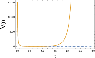
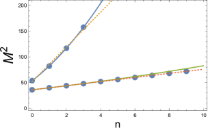
Figure 1: Left: We plot as a function of $t$ the potentials of the equivalent exact (solid), Eq.(10), and approximate (dotted), Eq.(12), Schrödinger equations. Right: We plot the glueball modes of the exact solution and approximate solution noticing that the latter is an almost linear relation with $M^{2}$ while the former is quadratic in mass in the region of our interest.

2.2 Mesons

In the case of the scalar mesons the variation of the action, Eq. (5), leads to

$$\partial_{M}(\sqrt{-g}e^{-\varphi(z)}g^{MN}\partial_{N}S(x,z))=\sqrt{-g}e^{-\varphi(z)(1-\alpha)}M^{2}_{5m}S(x,z).$$ (13)

Once we separate the $x$ dependence by factorizing $S(x,z)=\Sigma(z)e^{-iq_{\mu}x^{\mu}}$ with $q^{2}=-M^{2}$, where $M$ is the mass of the meson modes, we get

$$-\frac{d^{2}\Sigma(z)}{dz^{2}}+\left(\frac{3}{z}+2kz\right)\frac{d\Sigma(z)}{dz}+\frac{3}{z^{2}}e^{\alpha\varphi(z)}\Sigma(z)=M^{2}\Sigma(z)$$ (14)

where we have substituted the value of the scalar $AdS_{5}$ mass. By setting $\varphi(z)=kz^{2}$ and performing the change of function

$$\Sigma(z)=\left(\frac{z}{k}\right)^{\frac{3}{2}}e^{kz^{2}/2}\sigma(z),$$ (15)

we get a Schrödinger type equation

$$-\frac{d^{2}\sigma(z)}{dz^{2}}+\left(k^{2}z^{2}+2k+\frac{15}{4z^{2}}-\frac{3}{z^{2}}e^{\alpha kz^{2}}\right)\sigma(z)=M^{2}\sigma(z).$$ (16)

We now proceed to the change to the adimensional variable $u=\sqrt{k/2}\;z$,

$$-\frac{d^{2}\sigma(u)}{du^{2}}+\left(4u^{2}+4+\frac{15}{4u^{2}}-\frac{3}{u^{2}}e^{2\alpha u^{2}}\right)\sigma(u)=\Omega^{2}\sigma(u),$$ (17)

where $\Omega^{2}=(2/k)M^{2}$.

Let us perform the same approximation as before, namely to expand the exponential and keep up to three terms to obtain

$$-\frac{d^{2}\sigma(u)}{du^{2}}+\left((4-6\alpha)u^{2}+(4-6\alpha)+\frac{3}{4u^{2}}\right)\sigma(u)=\Omega^{2}\sigma(u).$$ (18)

This equation can be transformed into a Kummer type equation by the change of variables $v=(4-6\alpha^{2})^{1/4}u$

$$-\frac{d^{2}\sigma(v)}{dv^{2}}+\left(v^{2}+\frac{4-6\alpha}{\sqrt{4-6\alpha^{2}}}+\frac{3}{4v^{2}}\right)\sigma(v)=\frac{\Omega^{2}}{\sqrt{4-6\alpha^{2}}},$$ (19)

which has an exact spectrum given by

$$\Omega_{n}^{2}=4(n+1)\sqrt{4-6\alpha^{2}}+4-6\alpha,\;n=0,1,2,\ldots.$$ (20)

and the mode functions are

$$\sigma(v)=\mathcal{N}e^{-v^{2}/2}v^{3/2}{{}_{1}F_{1}}(-n,2,v^{2})$$ (21)

where $\mathcal{N}$ is a normalization factor and ${}_{1}F_{1}$ is a well known hypergeometric function and recall that $v=(4-6\alpha^{2})^{(1/4)}\;u$ where $u=(\sqrt{k/2}\;z)$. Note that the approximate solution only has bound states for $|\alpha|<\sqrt{2/3}$.

The meson modes are a function of $\alpha$. In the next section we will proceed to fix the parameters of the model by using phenomenological inputs. In the left panel of Fig. 2 we show the exact lowest mode for $\alpha=0.2$ (solid) together with the approximate solution obtained by expanding the exponential up to the third order (dotted). For small values of $\alpha$ both solutions are very similar and their mode values are almost equal. For larger values of $\alpha=0.4$ (see right panel of Fig. 2), closer to the no binding limit, the mode values are very similar but the exact solution becomes unstable. We shall discuss these details further in the next section.

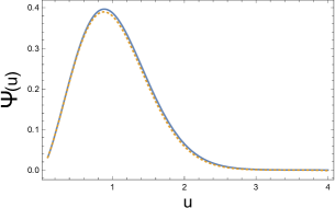
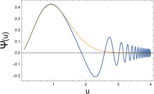
Figure 2: We plot as a function of $u$ for $\alpha=0.2$ (left) and $\alpha=0.4$ (right) the exact solution for the lowest mode (solid), Eq.(17), and the approximate lowest mode solution (dotted) obtained by expanding in the exact mode equation the exponential up to third order.

2.3 Phenomenological analysis

Our AdS/QCD model provides us with a succession of mass modes of differential equations which should be numerically solved. The equation for the glueballs Eq.(10) depends on a scale $\alpha k$ which we will use to match the glueball spectrum obtained from lattice QCD in the quenched approximation which is Gluodynamics  [21, 22, 23]. The equation for the mesons, Eq.(17), depends on $k$ and $\alpha$, separately. We use the PDG spectrum to fit the mesons spectrum [24, 25], which is certainly QCD, if we assume that QCD is the theory of the strong interactions. In principle, the scale of the glueballs and the mesons should be the same if we could fit QCD data, but since we are using lattice QCD in the quenched approximation to fit the latter, one could expect some minor differences between the two. We will choose the same mass scale. The fitting procedure is different from that used before by many authors [6, 12, 18] were an overall scale was used since in this case the scale affects the mode functions, which correspond to the light cone wave functions[8], through the relation between the $t$ and $z$ variables.

We proceed to fit the glueball spectrum. The used lattice data are shown in Table 2  [21, 22, 23] . We also use for the fit the results for the tensor glueball states since the theory predicts degeneracy between the scalar and the tensor glueball for all soft-wall models. The value of the parameter, obtained in the fit shown in Fig. 3 with the GSW model, is $\alpha k=(370$ MeV)². One should notice that the fit to the scalar glueball spectrum obtained by solving exactly the EoM leads to an almost linear relation between the mass and the mode number  [6].

$J^{PC}$	$0^{++}$	$2^{++}$	$0^{++}$	$2^{++}$	$0^{++}$	$0^{++}$
MP	$1730\pm 94$	$2400\pm 122$	$2670\pm 222$
YC	$1719\pm 94$	$2390\pm 124$
LTW	$1475\pm 72$	$2150\pm 104$	$2755\pm 124$	$2880\pm 164$	$3370\pm 180$	$3990\pm 277$

Table 2: Glueball masses [MeV] from lattice calculations by MP  [21], YC [22] and LTW  [23].

Meson	$f_{0}(500)$	$f_{0}(980)$	$f_{0}(1370)$	$f_{0}(1500)$	$f_{0}(1710)$	$f_{0}(2020)$	$f_{0}(2100)$	$f_{0}(2200)$
PDG	$475\pm 75$	$990\pm 20$	$1350\pm 150$	$1504\pm 6$	$1723\pm 6$	$1992\pm 16$	$2101\pm 7$	$2189\pm 13$

Table 3: Scalar meson masses [MeV] from PDG [24, 25].

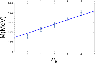
Figure 3: We plot the average lattice values for the scalar and tensor glueball masses of refs. [21, 22, 23] as a function of mode number. We show the fit to the spectrum from the modes of Eq. 10 by using just one parameter $\alpha k$.

Now that $\alpha k$ has been fixed, we will use $\alpha$ to fit the meson spectrum. In order to estimate the value of $\alpha$ let us use the approximate equation Eq.(19). From the mode equation Eq.(20) we get the spectrum

$$M_{n}^{2}=\Omega_{n}^{2}\dfrac{k}{2}=\Omega_{n}^{2}\dfrac{(370)^{2}}{2\alpha}~{}=A(\alpha)n+B(\alpha),$$ (22)

where $A(\alpha)=(740)^{2}\,(\sqrt{4-6\alpha^{2}}/2\alpha)$ and $B(\alpha)=(740)^{2}\;((\sqrt{4-6\alpha^{2}}+1-\frac{3}{2}\alpha)/2\alpha)$. Thus in the meson case our complicated equation of motion leads to a quadratic relation between mass and mode number, which is not the case for glueballs.

Having this analytic equation the fitting procedure is quite straightforward. The first question is if we should include the $f_{0}(500)$ in the fit. As discussed in our work [20], many authors have argued that this is not a conventional meson state but a tetraquark or a hybrid [34, 25]. In the present GSW model we have less freedom since the energy scale is fixed by the glueballs. In Fig. 4 we fit the PDG meson spectrum shown in Table 3 with our model. The left figure includes the $f_{0}(500)$ while the right figure does not.

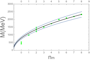
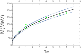
Figure 4: We plot the $f_{0}$ PDG meson spectrum [24, 25] as a function of mode number. Left panel: including the $f_{0}(500)$. The fits correspond to $\alpha=0.61$ (solid) and $\alpha=0.61\pm 0.04$ (dotted). Right panel: without the $f_{0}(500)$. The fits correspond to $\alpha=0.55$ (solid) and $\alpha=0.55\pm 0.04$ (dotted).

It is apparent again that the $f_{0}(500)$ is difficult to fit if the mass is so low as given in the PDG tables, and therefore, probably, the dynamical mechanism forming it is different from the rest of the mesons. From now on we will not consider the $f_{0}(500)$ in our fits to the meson spectrum.

The problem with the true solution, that corresponding to Eq.(17), is that it is very unstable as the binding potential becomes weaker, i.e. for values of $\alpha>0.2$ and much more unstable for the higher modes as shown in the right panel of Fig. 2. However, the spectrum does no differ much from the approximate spectrum and the mode functions have a similar structure before the large $u$ oscillations appear. One should notice that the value for which the approximate solution starts to be different from the exact solution, $u>1.5$, corresponds to $z>10/\Lambda_{QCD}$. Thus for a strong confined system such region is of little relevance. In Fig. 5 we analyse the behaviour of the mode values of the true solution. The dots represent the true solution. The upper points have been calculated for $\alpha=0.1$ and the lower points for $\alpha=0.2$. The lines represent the mode values of the approximate solution for $\alpha=0.1$ (solid) and $\alpha=0.3$ (dotted). Thus we see an almost perfect fit for $\alpha=0.1$ but for $\alpha=0.2$ the higher modes of the exact solution tends towards higher values of $\alpha$ of the approximate solution. If we look back to the right plot of Fig. 4 this is exactly what is happening, the lower values of the meson spectrum are fitted quite well by the approximate solution for $\alpha=0.51$, while the upper modes are fitted by the solution for $\alpha=0.59$. Having in mind these caveats from now on we will work with the approximate equation plotting not single curves but bands which take into account the difference between the true solution and the approximate one. The latter can be considered as the theoretical error in our approach.

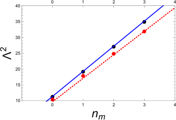
Figure 5: The dots represent the mode values of the true solution. The upper points correspond to $\alpha=0.1$, the lower points to $\alpha=0.2$. The lines represent the mode values of the approximate solution. The solid curve for $\alpha=0.1$ the dotted curve for $\alpha=0.3$.

One may conclude from the above analysis that the GSW model describes well both the scalar glueball and meson spectra with the same scale $\alpha k$. Let us remark that the energy scale arises from the metric as does the $\alpha$ modification which builds up the mesons. It is worth noticing that the value of $\alpha$ obtained from our phenomenological analysis for mesons is very close to the value of $\alpha$ obtained in Ref. [31] from a theoretical analysis developed for glueballs. In addition the dilatonic constant $\sqrt{k}=0.5$ GeV is extremely close to the values reported in Refs. [16, 36], i.e. $M_{\rho}/\sqrt{2}$. Let us recall that this fit is $\mathcal{O}(N_{C}^{0})$ and that corrections $\mathcal{O}(N_{C}^{-1})$ and higher should be added to obtain a precise value. However, the fact that the fit is quite good suggests that the contribution of the higher terms might be small.

Now that we have shown that our model describes well both spectra, a comment is necessary to highlight the importance of the structure of the metric. We have seen that the glueball spectrum in the region under scrutiny here has an almost linear relation between the mass and the mode number and this result is produced by our equations of motion (7) which cannot be approximated by a Kummer type equation as previously discussed. On the other hand, the meson equation, which is quite similar in structure to that of the glueball equation, acquires an $\alpha$ in the exponent of the exponential potential term. The value of $\alpha$ is crucial to allow for binding, but in so doing transforms the mode equation into an almost Kummer type equation with a quadratic relation between the mass and the mode number, as the experimental data indicate.

Now that we have an equation for the scalar mesons in the light sector, is it possible to generalize the equation to incorporate the heavy masses. In order to reproduce the heavy spectrum we have to add to the dynamics the mass of the heavy quarks. Several procedures are available [37, 38, 19] and we choose at this moment a very simple ansatz, namely to add a constants to the mass equation, which will be proven to be successful,

$$M_{n}=\sqrt{A(\alpha)n+B(\alpha)}+C,$$ (23)

where $C$ is the contribution of the quark masses, thus there will be a $C_{c}$ for the $c\bar{c}$ states and a different one $C_{b}$ for the $b\bar{b}$ states. In table 4 we show the values of the heavy scalar mesons masses collected by PDG  [24, 25]. It must be noted that some of the states do not have confirmed quantum numbers and others states themselves need to be confirmed.

			Scalar	Heavy	Mesons
$c\bar{c}$	$\chi_{c0}(1P)$	$\chi_{c0}(3860)$	$X(3915)$	$X(3940)$	$X(4160)$	$X(4350)$	$\chi_{c0}(4500)$	$\chi_{c0}(4700)$
$I^{G}(J^{PC})$	$0^{+}(0^{++})$	$0^{+}(0^{++})$	$0^{+}(0/2^{++})$	$?^{?}(?^{??})$	$?^{?}(?^{??})$	$0^{+}(?^{??})$	$0^{+}(0^{++})$	$0^{+}(0^{++})$
PDG	$3414\pm 0.30$	$3862^{+66}_{-45}$	$3918\pm 1.9$	$3942^{+13}_{-12}$	$4156^{+40}_{-35}$	$4350^{+5.3}_{-5.1}$	$4506^{+42}_{-41}$	$4704^{+24}_{-34}$
$b\bar{b}$	$\chi_{b0}(1P)$	$\chi_{b0}(1P)$
$I^{G}(J^{PC})$	$0^{+}(0^{++})$	$0^{+}(0^{++})$
PDG	$9859\pm 0.73$	$9912.21\pm 0.57$

Table 4: Heavy scalar meson spectrum [MeV] from PDG [25]. Notice that some of the particles are only suspected to be scalars and others need confirmation.

We show in Fig. 6 the fit obtained by Eq.(23) with the following parametrization. We have kept $\alpha$ fixed to the same values for all mesons, i.e. $\alpha=0.55$ (solid) and $\alpha=0.55\pm 0.04$ (dotted) and we have chosen for the light quark systems $C=0$, $C_{c}=2400$ MeV, for the $c\bar{c}$ mesons, and for the $b\bar{b}$ mesons $C_{b}=8700$ MeV. The fits are excellent given the simplicity of the model and moreover, and this is very exciting, $C_{c}\sim 2m_{c}$ and $C_{b}\sim 2m_{b}$. The heavy mesons have not been used at all to fit $\alpha$ and the model is showing that within its simplicity it is capable to reproduce, quite nicely, the scalar meson spectrum and therefore giving a lot of credibility to the glueball spectrum and the GSW model itself. Moreover we see that all mesons satisfy approximately the same mass trajectories apart from an overall scale associated with the quark masses and that all the elements in the PDG suspected of being scalar mesons seem to be scalar mesons. The model has proven to be tremendously predictive.

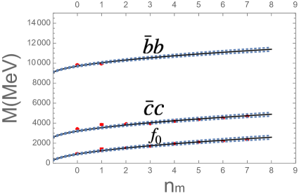
Figure 6: We show the scalar meson spectrum for all quark sectors. The light dots represent the scalar meson spectrum obtained from experimental data  [24, 25]. The curves correspond to Eq. (23) with $C_{c}=2400$ MeV for the $c\bar{c}$ mesons and $C_{b}=8700$ MeV for the $b\bar{b}$ mesons and the same two values of $\alpha$, i.e. $0.55$ (solid) and $0.55\pm 0.04$ (dotted) for all mesons.

3 Glueball-Meson mixing

In this section we provide an interpretation of the Mixing mechanism within a unified holographic description. In fact, as described in several analyses, see, e.g., Refs. [34, 39, 40, 41, 42], glueballs states can mix with mesons with similar masses and quantum numbers. Such an effect prevents a clear and safe extraction of the glueball spectra from data. It is therefore fundamental to provide a detailed description of the mixing effect in order to identify kinematic conditions where glueball states disentangle from those of mesons. In Fig. 7 we show the glueball lattice data (upper points) and the meson data (lower points). We plot also the fits with the GSW model discussed before and extend the fits to higher mode numbers to find that glueball masses with a certain mode number are equal to meson masses with a much larger mode number. For example, the glueball masses for $n_{g}=0,1,2$ are similar to the scalar meson masses for $n_{m}=4,7,10$ respectively. The difference in mode numbers grows as the masses of the glueballs increase due to the different slopes of the fitting curves. This observation has led us to discuss the meson glueball mixing scenario for high hadron masses in a recent paper [20]. We proceed to analyze the consequences of that observation in unified framework, by using the GSW model.

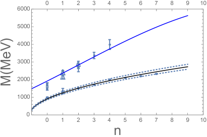
Figure 7: We show fits to the glueball spectrum (solid upper line) and scalar meson spectrum (lower band) obtained within the GSW model. The dark dots represent glueball spectrum obtained from lattice QCD [21, 22, 23]. The light dots represent the scalar meson spectrum obtained from experimental data  [24, 25]. We have extended the fits to high mode numbers to motivate our analysis of mixing.

Scalar glueballs might mix with scalar mesons [34, 39]. Recently, in view of the spectra of mesons and glueballs in AdS/QCD models, we have discussed the possibility that at high energies mixing might not be favorable and states with mostly gluonic valence structure might exist [20]. This is an exciting possibility since the presence of almost pure glueball states and the study of their decays would help in understanding many properties of QCD related to the physics of gluons. In here we have described an AdS/QCD model in the scalar sector that describes both scalar mesons an scalar glueballs on an equal footing by means of a unique energy scale. This energy scale enters the description of the mode functions which can be interpreted, in the previously developed scheme, as a light cone wave functions.

In order to investigate mixing between meson and glueball states we make use, in this section, of the Light-Front (LF) AdS/QCD formalism, see Ref. [43] for a useful review. In this formalism the equations of motion which describe the propagation of modes in anti-de Sitter space is taken to be equivalent to the equation for the light-front wave function for hadrons [44]. This approach has been successfully applied to describe several observable related to the non perturbative features of QCD such as decay constants, form factors, parton distribution functions (PDFs), generalised PDFs, transverse momentum dependent PDF and gravitational form factors [44, 45, 46, 47, 48, 49, 36, 50, 14, 15]. As shown in [48], the LF Holography matches the QCD running coupling in both the perturbative and non perturbative regions. Moreover, also the description of the $\rho$ meson electroproduction via LF AdS/QCD matches the data [36]. Due to all these remarkable results, we proceed to use LF AdS/QCD to describe the LF wave functions of glueballs and mesons calculated in terms of the solutions of the mode equations in the gravity sector

The holographic light-front representation of the equation of motion, in $AdS$ space can be recast in the form of a light-front Hamiltonian [8]

$$H_{LC}|\Psi_{n}>=M^{2}|\Psi_{n}>.$$ (24)

In the AdS/QCD light-front framework the above relation becomes a Schrödinger type equation

$$\left(-\frac{d^{2}}{dt^{2}}+V(t)\right)\Psi(t)=\Lambda^{2}\Psi(t)$$ (25)

where $t$ and $\Lambda^{2}$ in this equation are adimensional. The holographic light-front wave function are defined by $\Psi_{n}(t)=\;<t|\Psi_{n}>$ and are normalized as

$$<\Psi_{n}|\Psi_{n}>=\int dt|\Psi_{n}(t)|^{2}=1$$ (26)

The described mode functions introduce, in this way, probability distributions.

The eigenmodes of Eq.(25) determine the mass spectrum. In this framework, we get functions of $t$ for which we can define a probability distributions as in Eq.(26). In ref. [20] we discussed the mixing in a two dimensional Hilbert space generated by a meson and a glueball states, {$|\Psi_{m}>,|\Phi_{g}>$}. We found out that the mixing probability is proportional to the overlap probability of these two wave functions, i.e $|<\Psi_{m}|\Phi_{g}>|^{2}$ . Thus, in order to discuss the mixing, we need the mode functions. In the case of the glueballs we find the mode functions numerically since we have shown that the approximate solution is very different from the exact one, while in the meson case we use the approximate solution, which behaves similarly, with some caveats, to the exact mode function. The meson equation can be brought into Kummer’s form Eq.(19) by a convenient change of variables in terms of which the the mode functions are given by Eq.(21).

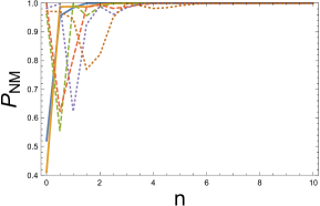
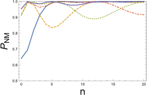
Figure 8: We plot the probability of no mixing as function of the meson mode number, $n$, and fixed glueball mode numbers. Left panel: $n_{g}=0$ (solid), $1$ (dashed), $3$ (dotted). Results have been obtained when both glueball and meson wave functions have been calculated within the same GSW model. We plot two lines for each $n_{g}$, one calculated with the meson wave function for $\alpha=0.51$ and the other calculated with the wave function for $\alpha=0.59$. Right Panel: $n_{g}=0$ (solid), $1$ (dashed), $2$ (dotted), $3$ (dot-dashed), $4$ (solid). Results have been obtained by using the GSW model to evaluate the glueball w.f. and the SW model for that of the meson, see Ref. [20].

In Fig. 8 we plot the probability of no mixing for low lying glueball modes ($n_{g}=1,2,3$) overlapping with mesons of modes up to mode number $n_{m}=10$. We observe that the overlap probability is small for the larger meson mode numbers and that it is only sizeable when the mode numbers of the two states are not very different. Let us make the discussion more detailed with an example. We choose a glueball of mode number $n_{g}=2$ and a meson of mode number $n=10$. They can be considered as candidates for mixing because the glueball mass in the model is $m(n_{g}=2)\sim 2800$ MeV and the meson mass is also $m(n_{m}=10)\sim 2800$ MeV. Thus this example is a prototype for a mixing scenario for heavy particles. In Fig.9 we show the mode functions for the $n_{g}=2$ glueball mode and that for the $n_{m}=10$ meson mode for the GSW model as a function of $t$. We notice that the meson function oscillates rapidly due to its larger mode number and therefore the overlap integral becomes very small. Note that the true mode function will be in between those two drawn, closer to the one of shorter wavelength for low modes and to the one of longer wavelength for the higher modes.

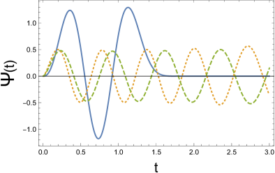
Figure 9: We plot the glueball mode function for $n_{g}=2$ and the meson mode functions for $n_{m}=10$ and $\alpha=0.51$ (dashed) and $\alpha=0.59$ (dotted).

Looking at Figs. 7 and left panel of Fig. 8, we see that a favorable mixing scenario is mostly excluded in the case of heavy glueballs and mesons, since the mass condition is satisfied for very different mode numbers. For example it can be seen that for $n_{g}=2,3,4$ the favorable meson modes of almost equal masses occur for $n\sim 10,13,17$. By comparing the left and right panels of Fig. 8, one can notice that only a unified description of glueballs and mesons within the same holographic model predicts a highly picked probability of mixing for low mode numbers and an extremely small probability for mode numbers that differ in several units. In fact, once the unified GSW model is adopted, for $n_{g}\leq 3$ then the mixing probability is negligible for $n_{m}\geq 3$. On the contrary, if one uses two different models, a tail at large $n_{m}$ can be found. The outcome of our analysis is that the AdS/QCD approach predicts the existence of almost pure glueball states in the scalar sector in the mass range above $2$ GeV.

4 Conclusion

In this work we have discussed the application of Graviton Soft Wall Model for both scalar glueballs and mesons. To this aim, we have initially compared the theoretical spectrum with lattice $QCD$ data in the case of the glueballs and the experimental $f_{0}$ spectrum of the PDG tables in the case of the mesons. The model introduces a unique energy scale for both glueballs and mesons. We have shown that the model respects the Regge behaviour and nicely reproduces both these spectra at leading order in $1/N_{c}$. How Regge behaviour comes about for the mesons is critically dependent on the value of the metric as described by the parameter $\alpha$. In our approach, the intrinsic Regge behaviour of the meson spectrum is a direct consequence of the metric and on the specific value of the parameter $\alpha$. The non linear equation obtained for the spectrum changes from a linear dependence on the mass to a quadratic dependence on the mass with the value of this parameter. In the latter case the non linear equation can be approximated by a Kummer type equation while in the former not. Thus the beauty of the model resides in that with similar equations it is able to reproduce the almost linear slope of the glueball spectra and the quadratic Regge trajectory for mesons. Moreover, the value of $\alpha$, obtained by fitting the meson spectrum $\sim 0.55\pm 0.04$ is very similar to that obtained by theoretical arguments from the glueball spectrum [31]. In addition, we remark that also the dilatonic constant we found is extremely close to that reported in Refs. [16, 36]. We have extended the model to the heavy quarks sector simply by adding a constant related to the quark masses to our equation for the spectrum as justified by other authors. The result of the analysis is excellent. Thus, the model is able to explain, within the limits of the leading $1/N_{C}$ dominance, all the scalar sector and moreover, predicts that some particles, whose quantum numbers are not known or need confirmation, are scalars or tensors.

We have noted that in our model the slope of the glueball spectrum, as a function of mode number, is also bigger than that of the meson spectrum and therefore for heavy almost degenerate glueballs and light quark mesons states their mode numbers differ considerably. Assuming a light-front quantum mechanical description of AdS/QCD correspondence, we have shown that the overlap probability of these heavy glueballs to heavy light quark mesons is small and thus one expects little mixing in the relatively high mass sector. Therefore, this is the kinematical region to look for almost pure glueball states. At present stage, large statistics of Central Exclusive Process (CEP) data is being collected by the LHC experiments, and we expect exciting new results to appear concerning the higher mass gluon enriched process.

References

- [1] J. M. Maldacena, Int. J. Theor. Phys. 38, 1113 (1999)
- [2] E. Witten, Adv. Theor. Math. Phys. 2, 505 (1998)
- [3] H. Fritzsch, M. Gell-Mann and H. Leutwyler, Phys. Lett. 47B (1973) 365.
- [4] H. Fritzsch and P. Minkowski, Phys. Lett. 56B (1975) 69.
- [5] V. Vento, Eur. Phys. J. A 53 (2017) no.9, 185
- [6] M. Rinaldi and V. Vento, Eur. Phys. J. A 54, 151 (2018)
- [7] J. Polchinski and M. J. Strassler, hep-th/0003136.
- [8] S. J. Brodsky and G. F. de Teramond, Phys. Lett. B 582 (2004) 211
- [9] L. Da Rold and A. Pomarol, Nucl. Phys. B 721 (2005) 79
- [10] A. Karch, E. Katz, D. T. Son and M. A. Stephanov, Phys. Rev. D 74 (2006) 015005
- [11] J. Erlich, E. Katz, D. T. Son and M. A. Stephanov, Phys. Rev. Lett. 95 (2005) 261602
- [12] P. Colangelo, F. De Fazio, F. Giannuzzi, F. Jugeau and S. Nicotri, Phys. Rev. D 78 (2008) 055009
- [13] G. F. de Teramond and S. J. Brodsky, Phys. Rev. Lett. 94, 201601 (2005).
- [14] M. Rinaldi, Phys. Lett. B 771, 563 (2017)
- [15] A. Bacchetta, S. Cotogno and B. Pasquini, Phys. Lett. B 771, 546 (2017)
- [16] G. F. de Teramond et al. [HLFHS Collaboration], Phys. Rev. Lett. 120, no. 18, 182001 (2018)
- [17] P. Colangelo, F. De Fazio, F. Jugeau and S. Nicotri, Phys. Lett. B 652 (2007) 73
- [18] E. Folco Capossoli and H. Boschi-Filho, Phys. Lett. B 753, 419 (2016)
- [19] S. Afonin and I. Pusenkov, Phys. Lett. B 726 (2013), 283-289
- [20] M. Rinaldi and V. Vento, J. Phys. G 47, no. 5, 055104 (2020)
- [21] C. J. Morningstar and M. J. Peardon, Phys. Rev. D 60 (1999) 034509
- [22] Y. Chen, A. Alexandru, S. J. Dong, T. Draper, I. Horvath, F. X. Lee, K. F. Liu and N. Mathur et al., Phys. Rev. D 73 (2006) 014516
- [23] B. Lucini, M. Teper and U. Wenger, JHEP 0406 (2004) 012
- [24] C. Patrignani et al. [Particle Data Group], Chin. Phys. C 40 (2016) no.10, 100001.
- [25] M. Tanabashi et al. [Particle Data Group], Phys. Rev. D 98 (2018) no.3, 030001 and 2019 update.
- [26] A. Vega and P. Cabrera, Phys. Rev. D 93, no. 11, 114026 (2016)
- [27] T. Akutagawa, K. Hashimoto and T. Sumimoto, arXiv:2005.02636 [hep-th].
- [28] T. Gutsche, V. E. Lyubovitskij, I. Schmidt and A. Y. Trifonov, Phys. Rev. D 99, no. 5, 054030 (2019)
- [29] I. R. Klebanov and J. M. Maldacena, Int. J. Mod. Phys. A 19, 5003 (2004)
- [30] M. A. Martin Contreras and A. Vega, Phys. Rev. D 101, no. 4, 046009 (2020)
- [31] E. Folco Capossoli, M. A. M. Contreras, D. Li, A. Vega and H. Boschi-Filho, [arXiv:1903.06269 [hep-ph]].
- [32] A. E. Bernardini, N. R. F. Braga and R. da Rocha, Phys. Lett. B 765, 81 (2017)
- [33] D. Li and M. Huang, JHEP 1311, 088 (2013)
- [34] V. Mathieu, N. Kochelev and V. Vento, Int. J. Mod. Phys. E 18 (2009) 1
- [35] E. Gregory, A. Irving, B. Lucini, C. McNeile, A. Rago, C. Richards and E. Rinaldi, JHEP 1210 (2012) 170
- [36] J. R. Forshaw and R. Sandapen, diffractive rho meson electroproduction,” Phys. Rev. Lett. 109, 081601 (2012)
- [37] T. Branz, T. Gutsche, V. E. Lyubovitskij, I. Schmidt and A. Vega, Phys. Rev. D 82 (2010), 074022
- [38] Y. Kim, J. Lee and S. H. Lee, Phys. Rev. D 75 (2007), 114008
- [39] V. Vento, Eur. Phys. J. A 52 (2016) no.1, 1
- [40] C. Amsler and F. E. Close, Phys. Rev. D 53, 295 (1996)
- [41] F. E. Close and N. A. Tornqvist, J. Phys. G 28, R249 (2002)
- [42] M. S. Chanowitz and S. R. Sharpe, Nucl. Phys. B 222, 211 (1983) Erratum: [Nucl. Phys. B 228, 588 (1983)].
- [43] L. Zou and H. Dosch, [arXiv:1801.00607 [hep-ph]].
- [44] S. J. Brodsky and G. F. de Teramond, Phys. Rev. Lett. 96, 201601 (2006)
- [45] S. J. Brodsky and G. F. de Teramond, Phys. Rev. D 77, 056007 (2008)
- [46] S. J. Brodsky and G. F. de Teramond, Phys. Rev. D 78, 025032 (2008)
- [47] G. F. de Teramond and S.J. Brodsky, Phys. Rev. Lett. 102, 081601 (2009)
- [48] S. J. Brodsky, G. F. de Teramond and A. Deur, Phys. Rev. D 81, 096010 (2010)
- [49] A. Vega, I. Schmidt, T. Branz, T. Gutsche and V. E. Lyubovitskij, Phys. Rev. D 80, 055014 (2009)
- [50] D. Chakrabarti, T. Maji, C. Mondal and A. Mukherjee, Phys. Rev. D 95, no. 7, 074028 (2017)