Mimetic Black Strings

Abstract

We present two new classes of black string solutions in the context of mimetic gravity. The horizon topology of these solutions can be either a flat $T^{2}$ torus with topology $S^{1}\times S^{1}$, or a standard cylindrical model with topology $R\times S^{1}$. The first class describes uncharged rotating black string which its asymptotic behavior is a quotient of anti-de Sitter (AdS) space, while the second class represents asymptotically AdS charged rotating black string. We study the casual structure and physical properties of these spacetimes and calculate, the entropy, electric charge, mass and angular momentum per unit length of rotating black strings.

1 Introduction

The idea of the mimetic gravity was proposed Mim1 , in order to shed the light on the problem of dark matter. Roughly speaking, isolating the conformal degree of freedom of the gravitational field in a covariant way, it was shown that the conformal degree of freedom can be dynamical even in the absence of matter. As a result, the extra scalar longitudinal degree of freedom of the gravitation field, can be interpreted as the energy density of the mimetic field which scales in term of the scalae factor $a$, as $a^{-3}$, which resembles the contribution of pressureless dust, without needing to particle dark matter Mim1 . In the past few years, mimetic theory of gravity has arisen a considerable attentions both in the cosmological setup as well as in stationary background. Cosmological dynamics of mimetic gravity, with various form of the potential for the mimetic field, has been investigated MimCos ; Dutta . It has been confirmed that this scenario can describe the thermal history of the universe, namely the successive sequence of radiation, matter, and dark-energy eras Dutta . Besides, at late times, mimetic cosmology is capable to alleviate the cosmic coincidence problem and can be brought into good agreement with observational data Dutta . It has been realized that with modification to the action of mimetic gravity, this model can address the singularities in contracting Friedmann and Kasner universes and yields a universe with limiting curvature and regular bounce MimCos1 . Considering the coupling between mimetic scalar field with a vector field, an anisotropic model of mimetic cosmology was explored in Sep . While inflationary model in the context of mimetic $f(G)$ gravity has been explored Zh , a unified description of dark energy and dark matter in the context of mimetic theory was suggested in Mat . Other studies on the mimetic cosmology can be found in Odin0 ; Odin1 ; Odin2 ; MimCos2 ; Gorj1 ; Gorj2 ; Gorj3 ; Gorj4 ; Leb ; Cham2 .

Parallel to the mimetic cosmology, the studies on static and stationary solutions of mimetic gravity started and have also being continued. Static and spherically symmetric black hole solutions of mimetic gravity have been explored in Myr1 ; Myr2 . The studies have also been generalized to modified Gauss-Bonnet mimetic gravity OdinGB as well as $f(R)$ mimetic theory OdinP ; Odinfr1 ; Odinfr2 ; Oik . In particular, it has been realized that, by suitably chosen mimetic potential for a given $f(R)$ gravity, this model admits an inflationary cosmology compatible with Planck observations OdinP . It was also observed that by modifying the action of mimetic gravity, a regular black hole can be exist without singularity inside the Schwarzschild spacetime Cham3 . Topological black holes in mimetic gravity in the presence of constant potential for the mimetic field were recently obtained in ShSa . By gluing an exterior static solution to a time-dependent anisotropic interior solution, the authors of Gorji2 constructed mimetic black hole spacetime. They also revealed that these two solutions match continuously on the event horizon Gorji2 . The authors of Nash1 ; Nash2 considered static and rotating solutions of mimetic gravity with flat or cylindrical horizon in the presence of cosmological constant. However, the obtained solution in Nash1 ; Nash2 are indeed nothing but the well-known black brane/string solutions of Einstein gravity. The reason is that they have simply assumed $\textbf{g}_{tt}=-\textbf{g}^{rr}$, and arrived at a special solution of the mimetic field equations. In order to reflect the impact of the extra degree of freedom of the gravitational field equations, encoded in the mimetic scalar field, on the metric functions, one need to consider the more general spacetime with $\textbf{g}_{tt}\neq-\textbf{g}^{rr}$ Myr1 ; Myr2 ; ShSa ; Gorji2 ; Ch ; Nash3 ; Der . Other studies on mimetic gravity can be carried out in Bar ; Gol ; Lim ; Cha ; Mal ; jibril .

One of the main question concerning mimetic theory, is that whether this theory is capable to reproduce the inferred flat rotation curves of galaxies. It was shown that adding a non-minimal coupling between matter and mimetic field yields the appearance of an extra force and the resulting equations of motion in the weak field limit provides a Modified Newtonian Dynamics (MOND)-like MimMOND theory which may alleviate the flat rotation curves of spiral galaxies without needing to particle dark matter. Also, constructing the potential associated with the mimetic field, by applying an inverse approach, for a general static spherically symmetric spacetime, it has been shown that the corrections to the Schwarzschild spacetime could provide an explanation for the inferred flat rotation curves of spiral galaxies within the mimetic gravity framework Myr2 . More recently, it has been realized ShSa that one is capable to reproduce the flat galactic rotation curves, in the context of mimetic gravity, without neither modifying the action MimMOND nor taking into account a complicated potential for the mimetic field Myr2 . Indeed, the original theory of mimetic gravity Mim1 was proposed in such a way that it naturally mimics dark matter as a geometrical effect. It was argued that the origin of the responsible term for recovering the flat galactic rotation curves in a static spacetime, is exactly the one which mimics dark matter in the cosmological setup ShSa .

In this paper, we are going to construct the general rotating black string solutions in the context of mimetic gravity. The rotating solutions of the Einstein equation with a negative cosmological constant with cylindrical and toroidal horizons have been investigated in Lem1 . The extension to include the Maxwell field has been done and the static and rotating electrically charged black string have been considered in Lem2 ; Awad ; mhd ; mhdk . When the gauge field is in the form of nonlinear electrodynamics, rotating black string solutions have been explored in H ; HS . The studies on the rotating black strings were also generalized to dilaton gravity mhdF ; She1 , holographic superfluids Betti and $f(R)$ gravity She2 .

This paper is structured as follows. In Sec. 2, we introduce the action and basic field equations. In Sec. 3, we analyze rotating black string in the context of mimetic gravity. In Sec. 4, we generalize our study to the case of charged rotating mimetic black string. We finish with conclusion and discussion in Sec. 5.

2 Field equations

The action of mimetic gravity in the presence of mimetic potential is MimCos

$$S=\int{d^{4}x\sqrt{-{g}}\left[\mathcal{R}+{\lambda}(\partial^{\mu}\phi\partial_{\mu}\phi-\epsilon)-V(\phi)+\mathcal{L}_{m}\right]},$$ (1)

where $\mathcal{R}$ is the Ricci scalar curvature, $\lambda$ is the Lagrange multiplier, and $V=V(\phi)$ is the potential for the mimetic scalar field $\phi$. Here $\mathcal{L}_{m}=-F_{\mu\nu}F^{\mu\nu}$ is the Lagrangian of the Maxwell field, where $F_{\mu\nu}=\partial_{\mu}A_{\nu}-\partial_{\nu}A_{\mu}$ is the electromagnetic field tensor and $A_{\mu}$ is the gauge potential. Besides, $\epsilon=\pm 1$ depends on the spacelike or timelike nature of the vector field $\partial_{\mu}\phi$. $\epsilon=+1$ corresponds to spacelike vector field $\partial_{\mu}\phi$, while $\epsilon=-1$ indicates timelike $\partial_{\mu}\phi$. Through this paper we set $8\pi G_{N}=1$ and work in the metric signature $(-,+,+,+)$. From the variation of the above action with respect to $\lambda$, one immediately finds

$$g^{\mu\nu}\partial_{\mu}\phi\partial_{\nu}\phi=\epsilon.$$ (2)

This constraint imposes strong restriction on the functional form of $\phi$ which in general depends on the metric line elements of the underlying theory. This condition can also be understood by assuming the physical metric $g_{\mu\nu}$ to be a function of two variable; namely an auxiliary metric $\tilde{g}_{\mu\nu}$ plus a scalar field $\phi$ and redefine the metric as $g_{\mu\nu}=\epsilon(\tilde{g}^{\alpha\beta}\partial_{\alpha}\phi\partial_{\beta}\phi)\tilde{g}_{\mu\nu}$ Mim1 . Then, one can immediately recovers (2). It was argued that considering this non-invertible conformal/disformal transformation, increases the number of degrees of freedom in such a way that in addition to two transverse degrees of freedom describing gravitons, the gravitational field acquires an extra dynamical longitudinal mode Der ; Fir .

The equations of motion can be derived by varying the action with respect to the metric $g_{\mu\nu}$, the scalar field $\phi$, and the gauge field $A_{\mu}$. The result is

$${G}_{\mu\nu} = \lambda\partial_{\mu}\phi\partial_{\nu}\phi-\frac{1}{2}g_{\mu\nu}V(\phi)+T_{\mu\nu},$$ (3)

$$\nabla^{\mu}(\lambda\partial_{\mu}\phi)=-\frac{1}{2}\frac{dV(\phi)}{d\phi},$$ (4)

$$\partial_{\mu}\left(\sqrt{-g}F^{\mu\nu}\right)=0,$$ (5)

where the energy momentum tensor of the Maxwell field is given by

$$T_{\mu\nu}=2F_{\mu\gamma}F_{\nu}^{\ \gamma}-\frac{1}{2}g_{\mu\nu}F_{\alpha\beta}F^{\alpha\beta},$$ (6)

Now, we take the trace of Eq. (3), combining with Eq. (2), yields

$$\lambda=\epsilon\left(G-T+2V\right),$$ (7)

where $G=G^{\mu}_{\mu}$ and $T=T^{\mu}_{\mu}$ are, respectively, the trace of the Einstein tensor and energy momentum tensor. Inserting $\lambda$ in the field Eqs. (3) and (4), we arrive at

$${G}_{\mu\nu} = \epsilon(G-T+2V)\partial_{\mu}\phi\partial_{\nu}\phi-\frac{1}{2}g_{\mu\nu}V(\phi)+T_{\mu\nu},$$ (8)

$$\nabla^{\mu}[(G-T+2V)\partial_{\mu}\phi]=-\frac{\epsilon}{2}\frac{dV(\phi)}{d\phi}.$$ (9)

Our aim here is to construct rotating black string solutions of the above field equations and investigate their properties. The metric of four-dimensional rotating solution with cylindrical or toroidal horizons can be written as Lem1 ; Lem2 ; Awad

$$ds^{2} = -f(r)g^{2}(r)\left(\Xi dt-ad\varphi\right)^{2}+\frac{dr^{2}}{f(r)}+\frac{r^{2}}{l^{4}}\left(adt-\Xi l^{2}d\varphi\right)^{2}+\frac{r^{2}}{l^{2}}dz^{2},$$ (10)

$$\Xi^{2} = 1+\frac{a^{2}}{l^{2}},$$

where the constants $a$ and $l$ have dimensions of length and as we will see later, $a$ is the rotation parameter and $l$ can be interpreted as the AdS radius, in case of constant potential. Compared to the line element of the rotating black string of Einstein gravity Awad , here we introduce a new function $g(r)$ in the metric due to the extra degree of freedom of the gravitational field, encoded by mimetic field. By solving the field equations, the unknown functions $f(r)$ and $g(r)$ would be determined. In metric (10) the ranges of the time and radial coordinates are $-\infty<t<\infty$, $0\leq r<\infty$. We are going to consider solutions in mimetic gravity with cylindrical symmetry. This implies that the spacetimes admit a commutative two dimensional Lie group $G_{2}$ of isometries Lem2 . The topology of the two dimensional surface, $t$=constant and $r$ =constant, generated by $G_{2}$ can be (i) the flat $T^{2}$ torus model with topology $S^{1}\times S^{1}$ $[\rm{i.e.}\ G_{2}=U(1)\times U(1)]$, and $0\leq\varphi<2\pi$, $0\leq z<2\pi l$, (ii) the standard cylindrical model with topology $R\times S^{1}$ $[\rm{i.e.}\ G_{2}=R\times U(1)]$, and $0\leq\varphi<2\pi$, $-\infty<z<\infty$, and (iii) the infinite plane $R^{2}$ with $-\infty<\varphi<\infty$ and $-\infty<z<\infty$ (this planar solution does not rotate). Hereafter, we shall consider the topology (i) and (ii).

In the coordinate system with metric (10), the general solution to the constraint equation (2) become

$$f(r)\phi^{\prime 2}=\epsilon,\ \rightarrow\ \phi(r)=\pm\int{\frac{dr}{\sqrt{|\epsilon f(r)|}}}+\rm const,$$ (11)

where without loss of generality one may choose $+$ sign of integral. The scalar field is always constrained by Eq. (2) or, equality in our case, by Eq. (11). Therefore, we have no new degrees of freedom for the scalar field $\phi$. Indeed, this constrained scalar field is not dynamical by itself, but induces mimetic dark matter in Einstein theory making the longitudinal mode of gravity dynamical Mim1 . Let us remind that in the cosmological setup the vector field $\partial^{\mu}\phi$ is always timelike because it plays the role of the four-velocity $u^{\mu}$ of the perfect fluid, where $\phi$ is the velocity potential Mim1 . Indeed, in the background of Friedmann-Robertson-Walker universe the general solution of the constraint equation (2) is $\phi=\pm t+A$, where $A$ is an integration constant, and without loss of generality one can identify $\phi=t$ MimCos . However, in the context of black hole/string, where, by definition, the spacetime has an event horizon, the vector field $\partial_{\mu}\phi$ changes from a spacelike vector to a timelike vector over the horizon. However, since, the scalar field $\phi$ is not dynamical by itself, one may not worry about this behvaiour and can still search for black hole/string solutions with real $f(r)$.

Considering the metric (10), the gauge potential takes the form

$$A_{\mu}=h(r)\left(\Xi\delta_{\mu}^{0}-a\delta_{\mu}^{\phi}\right).$$ (12)

With this gauge potential at hand, the nonvanishing components of the electromagnetic tensor become

$$F_{tr}=\Xi h^{\prime}(r),\ \ \ \ \ F_{\varphi r}=-ah^{\prime}(r)=-\frac{a}{\Xi}F_{tr}.$$ (13)

Inserting the gauge potential (12) into Eq. (5), one finds that the non-vanishing components of the Maxwell equation are just the ($t$) and $(\varphi)$ components, which both of them yield the following equation

$$rh^{\prime\prime}(r)g(r)-rh^{\prime}(r)g^{\prime}(r)+2h^{\prime}(r)g(r)=0,$$ (14)

where by prime we denote $r$ derivative. The above equation admits the following unique solution

$$h^{\prime}(r)=\frac{q}{r^{2}}g(r),$$ (15)

where we denote the constant of integration by $q$, since it should be related to the electric charge of the black hole. Hence from (13), we obtain

$$F_{tr}=\Xi\frac{q}{r^{2}}g(r),\ \ \ \ F_{\varphi r}=-a\frac{q}{r^{2}}g(r).$$ (16)

Inserting metric (10), condition (11), and the electromagnetic fields (16) into the field equations (8), we arrive at the following equations for the non-vanishing components of the gravitational field equations

$$gl^{2}\Xi^{2}\left(2r^{3}f^{\prime}+2f{r}^{2}+V\left(\phi\right){r}^{4}+2{q}^{2}\right)+a^{2}g\left(-2r^{3}f^{\prime}-r^{4}f^{\prime\prime}-r^{4}V(\phi)+2q^{2}\right)$$

$$+a^{2}\left(-2r^{4}fg^{\prime\prime}-2r^{3}fg^{\prime}-3r^{4}f^{\prime}g^{\prime}\right)=0,$$ (17)

$$3\,{r}^{3}gf^{\prime}+2\,{r}^{3}fg^{\prime}+{r}^{2}gf+3\,{r}^{4}f^{\prime}g^{\prime}+2\,{r}^{4}fg^{\prime\prime}+{r}^{4}gf^{\prime\prime}+\frac{3}{2}{r}^{4}gV\left(\phi\right)-{q}^{2}g=0,$$ (18)

$$\Xi^{2}l^{2}\left[2\,{r}^{3}(fg)^{\prime}+3{r}^{4}f^{\prime}g^{\prime}+2{r}^{4}fg^{\prime\prime}+{r}^{4}gf^{\prime\prime}+{r}^{4}\,gV\left(\phi\right)-2\,{q}^{2}g\right]$$

$$-a^{2}g\left(2r^{3}f^{\prime}+2r^{2}f+{r^{4}}V(\phi)+2q^{2}\right)=0,$$ (19)

$$2\,{r}^{3}(fg)^{\prime}+3{r}^{4}f^{\prime}g^{\prime}+2{r}^{4}fg^{\prime\prime}+{r}^{4}gf^{\prime\prime}+{r}^{4}\,gV\left(\phi\right)-2\,{q}^{2}g=0,$$ (20)

$$\Xi a\left(3r^{4}f^{\prime}g^{\prime}-2gfr^{2}-4q^{2}g+2r^{3}fg^{\prime}+r^{4}gf^{\prime\prime}+2r^{4}fg^{\prime\prime}\right)=0.$$ (21)

Our aim here is to solve the above field equations and obtain the unknown functions $f(r)$ and $g(r)$. Clearly, our solutions should also satisfy Eq. (9) for the scalar field. During this paper we consider the case for which the potential is constant, namely, $V(\phi)=V_{0}=-2\Lambda$, where for later convenience we assume this constant to be positive definite, i.e. $\Lambda=3/l^{2}>0$.

Multiplying Eq. (20) by factor $\Xi^{2}l^{2}$ and subtracting the resulting equation from (2), we arrive at

$$r^{3}f^{\prime}+r^{2}f+\frac{r^{4}}{2}V(\phi)+q^{2}=0.$$ (22)

Substituting $V(\phi)=-2\Lambda$ in Eq. (22), and solving for $f(r)$, we find

$$f(r) = -\frac{m}{r}+\frac{q^{2}}{r^{2}}+\frac{\Lambda}{3}r^{2},$$ (23)

where $m$ and $q$ are integration constants which are, respectively, related to the mass and charge of the black string. Inserting solution (23) into Eq. (18), we find the following equation for the metric function $g(r)$:

$$(2\Lambda r^{5}-6mr^{2}+6q^{2}r)g^{\prime\prime}+(8\Lambda r^{4}+3mr-12q^{2})g^{\prime}=0.$$

Solving yields

$$g(r)=c_{1}+c_{2}\int{\frac{r^{2}dr}{(|\Lambda r^{4}-3mr+3q^{2}|)^{3/2}}},$$ (25)

where $c_{1}$ and $c_{2}$ are the constants of integration. In the limiting case where $c_{2}=0$, our solution is nothing but the corresponding one of Einstein gravity which is indeed the solution obtained in Nash1 . Without loss of generality we can set $c_{1}=1$. Indeed, the effects of $c_{1}$ in function (25) can be absorbed by rescaling $t\rightarrow t/c_{1}$ and $\varphi\rightarrow\varphi/c_{1}$ in the line element (10). Thus, we rewrite the general solution as

$$g(r)=1+b\int{\frac{r^{2}dr}{(|\Lambda r^{4}-3mr+3q^{2}|)^{3/2}}},$$ (26)

where $b$ is a constant which reflects the imprint of the mimetic field in the solutions. One can easily check that the obtained solutions (23) and (26) are fully satisfied the field equations (9) and (2)-(21). Since the integral in the function (26) cannot be calculated easily, we consider in the following two sections the uncharged and charged rotating black strings, separately.

3 Uncharged mimetic black string

In this case ($q=0$), the field Eq. (2) reduces to

$$(2\Lambda r^{5}-6mr^{2})g^{\prime\prime}+(8\Lambda r^{4}+3mr)g^{\prime}=0,$$ (27)

which admit the following solution

$$g(r)=1+\frac{b_{0}\ r^{3/2}}{\sqrt{|\Lambda r^{3}-3m}|},$$ (28)

where $b_{0}$ is a constant with dimension $[length]^{-1}$ which incorporates the imprint of the mimetic field on the spacetime metric. The horizon, by its definition, is a null hypersurface $\mathcal{S}$ at constant $r=r_{+}$, determined by $\textbf{g}^{rr}=0$ Townsend . For the black string spacetime under consideration, this implies $\textbf{g}^{rr}=f(r_{+})=0$ which, using (23) with $q=0$, leads to $r_{+}=(3m/\Lambda)^{1/3}$. The sign in the denominator of (28) depends on inner ($r<r_{+}$) or outer ($r>r_{+}$) part of the solutions. For $r>r_{+}$, $|\Lambda r^{3}-3m|=\Lambda r^{3}-3m$, while for $r<r_{+}$, $|\Lambda r^{3}-3m|=3m-\Lambda r^{3}$. The spacetime is regular for whole range $0<r<\infty$ and the divergency in $g(r)$ at $r=r_{+}$ is just a coordinate singularity and all scalar invariants are finite in the whole range $0<r<\infty$. Our solution is not static and the Killing vector

$$\chi=\partial_{t}+\Omega_{+}\partial_{\varphi},$$ (29)

is the null generator of the event horizon where $\Omega_{+}$ is the angular velocity of the event horizon. Since the Killing vector (29) is normal to the null hypersurface $\mathcal{S}$ ($r=r_{+}$), thus $\mathcal{S}$ is a Killing horizon of the Killing vector field Townsend . By analytic continuation of the metric we can obtain the surface gravity and angular velocity associated with the horizon. The analytical continuation of the Lorentzian metric by $t\rightarrow i\tau$ and $a\rightarrow ia$ yields the Euclidean section, whose regularity at $r=r_{+}$ requires that we should identify $\tau\sim\tau+\beta_{+}$ and $\phi\sim\phi+i\beta_{+}\Omega_{+}$ where $\beta_{+}$ and $\Omega_{+}$ are the inverse Hawking temperature and the angular velocity of the horizon Townsend . It is a matter of calculation to show that

$$\beta_{+} = \frac{4\pi\Xi}{g(r_{+})f^{\prime}(r_{+})},$$ (30)

$$\Omega_{+} = \frac{a}{\Xi l^{2}}.$$ (31)

Of course the temperature can also be calculated via surface gravity. The general definition of surface gravity is Wald

$$\kappa=\sqrt{-\frac{1}{2}(\nabla^{\mu}\chi^{\nu})(\nabla_{\mu}\chi_{\nu})},$$ (32)

where in our case, $\chi^{\nu}=(1,0,\Omega_{+},0)$ is the Killing vector (29) associated with the Killing horizon $\mathcal{S}$. A simple calculation for the spacetime (10) gives $\kappa=g(r_{+})f^{\prime}(r_{+})/(2\Xi)$.

One may also calculate the entropy associated with the horizon. The entropy of the black string still obeys the so called area law of the entropy which states that the entropy of the black hole is a quarter of the event horizon area. It is a matter of calculation to show that the entropy per unit length of the string is

$${S}=\frac{r_{+}^{2}\Xi}{4l}.$$ (33)

In order to see the asymptotic behavior of the solutions, we consider the non-rotating case ($a=0$), where the line elements of the black string is given by

$$ds^{2} = -f(r)g^{2}(r)dt^{2}+\frac{dr^{2}}{f(r)}+r^{2}d\varphi^{2}+\frac{r^{2}}{l^{2}}dz^{2}.$$ (34)

Therefore, the $(tt)$ component of the static black string is given by ${-\textbf{g}_{tt}(r)}=f(r)g^{2}(r)=B(r)$, where

$$B(r)=\left(-\frac{m}{r}+\frac{\Lambda r^{2}}{3}\right)\left[1+\frac{b_{0}\ r^{3/2}}{\sqrt{|\Lambda r^{3}-3m|}}\right]^{2}.$$ (35)

Expanding $g(r)$ and $B(r)$ for large values of $r$, we arrive at

$$g(r)\approx 1+\frac{b_{0}}{\sqrt{\Lambda}}+\frac{3mb_{0}}{2\Lambda^{3/2}r^{3}}+O\left(\frac{1}{r^{6}}\right),$$ (36)

$$B(r)\approx\frac{r^{2}}{3}\left(\Lambda+b_{0}^{2}+2b_{0}\sqrt{\Lambda}\right)-\frac{m}{r}\left(1+\frac{b_{0}}{\sqrt{\Lambda}}\right)+O\left(\frac{1}{r^{4}}\right).$$ (37)

Thus as $r\rightarrow\infty$, the spacetime is a quotient of AdS although its asymptotic behavior get modified due to the presence of the mimetic field $\phi$ which its imprint incorporates in the metric functions via the constant $b_{0}$. Nevertheless, by redefining $(\Lambda+b_{0}^{2}+2b_{0}\sqrt{\Lambda})\mapsto\Lambda^{\prime}$, one can easily realize that the solution given in (37) is asymptotically AdS.

It is also interesting to calculate the curvature scalars of this spacetime. Expanding the Ricci scalar and the Kretschmann invariant around $r=0$, we arrive at

$$\lim_{r\rightarrow 0}R=\frac{\rm const.}{\sqrt{r^{3}}}-4\Lambda+b_{0}^{2}+\cdot\cdot\cdot,$$ (38)

$$\lim_{r\rightarrow 0}R_{\mu\nu\rho\sigma}R^{\mu\nu\rho\sigma}=\frac{12m^{2}}{r^{6}}-\frac{17mb_{0}^{2}}{r^{3}}+\cdot\cdot\cdot$$

Thus, both curvature invariants diverge as $r\rightarrow 0$, which confirms that there is an essential singularity located at $r=0$. On the other side, for the asymptotic region where $r\rightarrow\infty$, the invariants of the spacetime are obtained as

$$\lim_{r\rightarrow\infty}R = -4\Lambda,$$ (39)

$$\lim_{r\rightarrow\infty}R_{\mu\nu\rho\sigma}R^{\mu\nu\rho\sigma} = \frac{8}{3}\Lambda^{2},$$ (40)

It is also easy to show that Ricci and Kretschmann invariants have finite values on the horizon $r_{+}$. Having a look on Eq. (35), one may wonder that at the horizon, the function $-\textbf{g}_{tt}(r)=B(r)$ diverge and the metric becomes singular. However, this is indeed not the case. Simplifying the metric function (35), it can be rewritten

$$B(r)=\frac{\left(\sqrt{\Lambda r^{3}-3m}+b_{0}r^{3/2}\right)^{2}}{3r}$$ (41)

which clearly has a finite value at $r_{+}$. Furthermore, from the above expression we observe that $B(r)$ is well-defined for $r>r_{+}$ and has a minimum value $B(r)\mid_{\rm min}=b_{0}^{2}r_{+}^{2}/3$ at the horizon.

One may also look for the surface where the redshift becomes infinite. The infinite redshift surface is the surface where clock intervals in flat space correspond to infinite time intervals on the infinite redshift surface. More precisely, for an emitter $E$ and receiver $R$ with fixed spatial coordinates in a stationary spacetime, the gravitational frequency shift of a photon is, quite generally, given by Hob

$$\frac{\nu_{R}}{\nu_{E}}=\left[\frac{\textbf{g}_{tt}(A)}{\textbf{g}_{tt}(B)}\right]^{1/2},$$ (42)

where $A$ is the event at which the photon is emitted and $B$ the event at which it is received. Thus, we see that if the photon is emitted from a point with fixed spatial coordinates, then $\nu_{R}\rightarrow 0$ in the limit $\textbf{g}_{tt}\rightarrow 0$, so that the photon suffers an infinite redshift. Thus a surface defined by $\textbf{g}_{tt}=0$ is also often called an infinite redshift surface. For the Schwarzschild spacetime, both an infinite redshift surface and event horizon coincide, but in more general axisymmetric spacetime such as Kerr black holes these surfaces do not coincide. In our case, by setting $-\textbf{g}_{tt}=B(r)=0$, we find that the surface of infinite redshift is given by

$$r_{s}=\left(\frac{3m}{\Lambda-b_{0}^{2}}\right)^{1/3}.$$ (43)

Thus the infinite redshift surface only exist provided we have $\Lambda>b_{0}^{2}$. It can be seen that for $b_{0}=0$ the infinite redshift surface coincides with the event horizon. This is indeed an expected result, since in this case our solutions reduce to black string solutions of Einstein gravity.

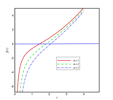
Figure 1: The behavior of $f(r)$ for rotating black string with $\Lambda=1$.

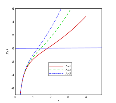
Figure 2: The behavior of $f(r)$ for rotating black string with $m=2$.

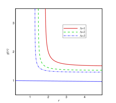
Figure 3: The behavior of $g(r)$ for rotating black string. Here we have taken $b_{0}=1/2$ and $m=2$.

The behaviour of the metric functions $f(r)$ and $g(r)$ are depicted in Figs. 1-3. From Figs. 1 and 2 we see that rotating black string in mimetic gravity has only one horizon at finite radius $r_{+}$ where $f(r)$ and hence $B(r)=f(r)g^{2}(r)$ change sign on it. We observe that with increasing $m$ or decreasing $\Lambda$, the radius of this horizon increases as well, which can be easily understood from its definition. Besides, as $r\rightarrow 0$, the metric function diverges, which confirm that there is a singularity at $r=0$ which already confirmed that it is indeed an essential singularity. Finally, from Fig. 3 it is observed that the function $g(r)$ approach to constant value $1+b_{0}/\sqrt{\Lambda}$ in large $r$ limit.

We finish this section by calculating the mass and angular momentum of the rotating mimetic black strings. We shall use the counterterm method inspired by AdS/CFT correspondence. In our case the suitable boundary term which removes the divergences of the action can be written

$$S_{b} = \frac{1}{8\pi}\int_{\partial\mathcal{M}}d^{3}x\sqrt{-\gamma}\left(\Theta(\gamma)+\frac{2}{l}\right),$$ (44)

where $\Theta$ is the trace of the extrinsic curvature $\Theta^{\mu\nu}$ for the boundary ${\partial\mathcal{M}}$ and $\gamma$ is the induced metric on the boundary. The second term in (44) is the the suitable counterterm. Variation of the action (44) with respect to boundary metric $\gamma_{\mu\nu}$ yields the following finite stress-energy tensor mhd

$$T^{ab}=\frac{1}{8\pi}\left[\Theta^{\mu\nu}-\Theta\gamma^{\mu\nu}+\frac{2}{l}\gamma^{\mu\nu}\right].$$ (45)

In order to compute the conserved charges of the spacetime, we choose a spacelike surface $\mathcal{B}$ in the boundary $\partial\mathcal{M}$ with metric $\sigma_{ij}$, and write the boundary metric in ADM (Arnowitt-Deser-Misner) form:

$$\gamma_{ab}dx^{a}dx^{a}=-N^{2}dt^{2}+\sigma_{ij}\left(d\varphi^{i}+V^{i}dt\right)\left(d\varphi^{j}+V^{j}dt\right),$$

where the coordinates $\varphi^{i}$ are the angular variables parameterizing the hypersurface of constant $r$ around the origin, and $N$ and $V^{i}$ are the lapse and shift functions respectively. For the Killing vector field $\mathcal{\xi}$ on the boundary, the quasilocal conserved quantities associated with the stress tensors of Eq. (45) are given by mhd

$$Q(\mathcal{\xi)}=\int_{\mathcal{B}}d^{2}x\sqrt{\sigma}T_{ab}n^{a}\mathcal{\xi}^{b},$$ (46)

where $\sigma$ is the determinant of the metric $\sigma_{ij}$, $\mathcal{\xi}$ and $n^{a}$ are, respectively, the Killing vector field and the unit normal vector on the boundary $\mathcal{B}$. For boundaries with timelike ($\xi=\partial/\partial t$) and rotational ($\varsigma=\partial/\partial\varphi$) Killing vector fields, one obtains the conserved mass and angular momenta of the system enclosed by the boundary $\mathcal{B}$ as mhd

$$M = \int_{\mathcal{B}}d^{2}x\sqrt{\sigma}T_{ab}n^{a}\xi^{b},$$ (47)

$$J = \int_{\mathcal{B}}d^{2}x\sqrt{\sigma}T_{ab}n^{a}\varsigma^{b}.$$ (48)

It is important to note that both $M$ and $J$ are independent of the particular choice of foliation $\mathcal{B}$ within the surface $\partial\mathcal{M}$ while they depend on the location of the boundary $\mathcal{B}$ in the spacetime. Then, it is a matter of calculations to show that the mass and angular momentum per unit length of the rotating string when $\mathcal{B}\rightarrow\infty$ are given by

$${M} = \frac{(3\Xi^{2}-1)m}{16\pi l}+\frac{b_{0}m\sqrt{3}}{24\pi},$$ (49)

$${J} = \frac{3\Xi\sqrt{\Xi^{2}-1}m}{16\pi},$$ (50)

where we have also used $\Lambda=3/l^{2}$. When $a=0$ ($\Xi=1$), the angular momentum per unit volume vanishes, which confirms that parameter $a$ is indeed the rotational parameters of the black string. Compared to the mass and angular momentum of black string solutions of Einstein gravity mhd ; Awad , we see that the angular momentum do not change, while the mass get an additional term. When $b_{0}=0$, the mass also reduces to the one of Einstein gravity mhd ; Awad .

4 Charged mimetic black string

Now we consider the general solutions given by (23) and (26). Since we are looking for the analytical solutions and the integral in (26) cannot be done analytically, we study the behaviour in two ranges. For large $r$, the dominant term in the integrand is $\Lambda r^{4}$ and we have

$$g(r) = 1+b\int{\frac{r^{2}dr}{(|\Lambda r^{4}-3mr+3q^{2}|)^{3/2}}}$$ (51)

$$\approx 1+\frac{b}{\Lambda^{3/2}}\int{\frac{dr}{r^{4}}}+\cdot\cdot\cdot\approx 1-\frac{b}{3\Lambda^{3/2}}\frac{1}{r^{3}}+\cdot\cdot\cdot$$ (52)

Thus the metric function $B(r)=f(r)g^{2}(r)$, for large $r$, is

$$B(r) = -\frac{m}{r}+\frac{q^{2}}{r^{2}}+\frac{\Lambda r^{2}}{3}-\frac{2b}{9\sqrt{\Lambda}}\frac{1}{r}+O\left(\frac{1}{r^{4}}\right),$$ (53)

which contains an additional term of $O(1/r)$ compared to charged rotating black string solution of Einstein gravity Awad . This term reflects the imprint of mimetic field on the spacetime. We observe that the asymptotic behaviour of the solutions is AdS which differs from the uncharged case where the spacetime was approximately asymptotically AdS. On the other hand when $r\rightarrow 0$, we can neglect the term $\Lambda r^{4}$ and the solution becomes

$$g(r) \approx 1+b\int{\frac{r^{2}dr}{(3q^{2}-3mr)^{3/2}}}\approx 1+\sqrt{3}b\left[2\left(\frac{2q}{3m}\right)^{3}+\left(\frac{r}{3q}\right)^{3}+\cdot\cdot\cdot\right],$$ (54)

and thus

$$B(r) \approx \left(-\frac{m}{r}+\frac{q^{2}}{r^{2}}+\frac{\Lambda r^{2}}{3}\right)\Bigg{\{}1+\sqrt{3}b\left[2\left(\frac{2q}{3m}\right)^{3}+\left(\frac{r}{3q}\right)^{3}+\cdot\cdot\cdot\right]\Bigg{\}}^{2}.$$ (55)

From (55) we observe that near the singularity where $r\rightarrow 0$ we have $B(r)\rightarrow\infty$, as one expected. When $b=0$, our solutions given in (53) and (55) reduce to asymptotically AdS charged black string of Einstein gravity.

The horizon can be obtained by solving $f(r)=0$, where $f(r)$ is given by Eq. (23). Thus, the horizons are the real root of equation $\Lambda r^{4}-3mr+3q^{2}=0$. Depending on the values of the parameters this equation may have zero, one or two roots. The cases with zero or one root correspond to naked singularity and extremal black hole, respectively. When this equation has two roots we encounter a black hole with two inner and outer horizon.

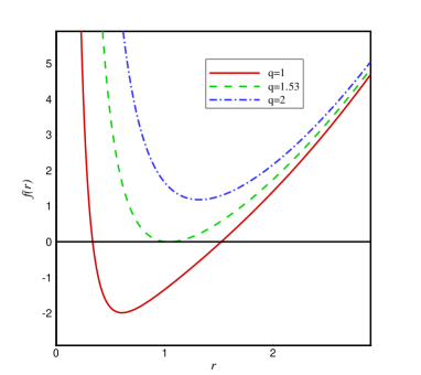
Figure 4: The behavior of $f(r)$ for charged rotating black string with different $q$, where we have taken $m=3$, $\Lambda=2$.

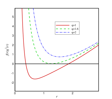
Figure 5: The behavior of $B(r)=f(r)g^{2}(r)$ for charged rotating black string given in Eq. (53) with different $q$. Here we have taken $m=2$, $b=3$ and $\Lambda=1$.

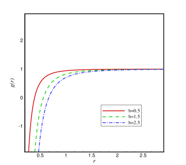
Figure 6: The behavior of $g(r)$ for charged rotating black string for large $r$ limit with $\Lambda=2$.

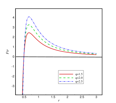
Figure 7: The behavior of $F_{tr}(r)$ for charged rotating black string for different $q$. Here we have taken $b=1$, $\Lambda=2$, $\Xi=1.2$.

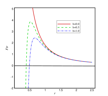
Figure 8: The behavior of $F_{tr}(r)$ for charged rotating black string for different parameter $b$. Here we have taken $q=1.5$, $\Lambda=2$, $\Xi=1.2$.

The behavior of the metric functions for charged rotating black string are depicted in Figs. 4-6. From Fig. 4, we see that, depending on the metric parameters, our solutions can represent black string with two horizons, an extremal black string or naked singularity. From Fig. 5, we also observe that our solutions admit two, one or zero surface of infinite redshift if the metric parameters are chosen suitably. We have also plotted the bahviour of $g(r)$ in Fig. 6, where it can be seen that $g(r)\rightarrow 1$ for large values of $r$ and goes to $-\infty$ as $r\rightarrow 0$.

Given the function $g(r)$, the explicit form of the electric field, for large $r$, is given by

$$F_{tr}=\frac{q\Xi}{r^{2}}\left[1-\frac{b}{3\Lambda^{3/2}}\frac{1}{r^{3}}+O\left(\frac{1}{r^{5}}\right)\right].$$ (56)

Let us note that for $b\neq 0$, the electric field has a maximum value at $r_{\rm max}=\left(\frac{5b}{6\Lambda^{3/2}}\right)^{1/3}$, and goes to zero as $r\rightarrow\infty$. This maximum value appears since the imprint of the mimetic field which contributes to the second negative term of (56) reduces the electric field compared to the case of Einstein gravity. Figs. 7 and 8 demonstrate the behaviour of the electric field $F_{tr}(r)$ for charged rotating mimetic black strings. From these figures we observe that the maximum value of electric field increases with increasing $q$, while it decreases and shifts to larger $r$ with increasing $b$. This can be understood since for larger $b$ the effects of the mimetic field makes the electric field weaker. The large $r$ limit behaviour of the metric functions as well as $F_{tr}(r)$ and $F_{\varphi r}(r)$ indicate that far from the black string $(r\gg r_{+})$, the effects of the mimetic field disappear and one recovers the Einstein gravity up to a constant.

We then look for the curvature singularity. To do that, we expand the scalar invariants for the obtained solutions,

$$\lim_{r\rightarrow 0}R=-\frac{126q^{2}}{r^{4}}+\cdot\cdot\cdot$$ (57)

$$\lim_{r\rightarrow 0}R_{\mu\nu\rho\sigma}R^{\mu\nu\rho\sigma}=\frac{26124q^{4}}{r^{8}}+\cdot\cdot\cdot$$ (58)

Therefore, we have an essential singularity located at $r=0$. On the other side, for the asymptotic region where $r\rightarrow\infty$, the invariants of the spacetime are obtained as

$$\lim_{r\rightarrow\infty}R=-4\Lambda,$$ (59)

$$\lim_{r\rightarrow\infty}R_{\mu\nu\rho\sigma}R^{\mu\nu\rho\sigma}=\frac{8}{3}\Lambda^{2}.$$ (60)

In order to calculate the mass and angular momentum of charged rotation black string, we use the method of the previous section. In this case the mass and angular momentum per unit length of the charged rotating black string are given by

$${M} = \frac{(3\Xi^{2}-1)m}{16\pi l}+\frac{b(\Xi^{2}-1)\sqrt{3}}{72\pi},$$ (61)

$${J} = \frac{\Xi\sqrt{\Xi^{2}-1}(27m+2\sqrt{3}bl)}{144\pi}.$$ (62)

When $b=0$, the above expressions for the mass and angular momentum restore their respective expressions in Einstein gravity. Let us note that $M$ and $J$ differ for charged and uncharged rotating black strings. This may due to the fact that the asymptotic behaviour of these two classes of solutions are different. For the uncharged string, the asymptotic behaviour is approximately AdS, while for charged rotating string, the solutions are asymptotically AdS. However, this issue deserves further investigation.

Finally, we calculate the electric charge of the mimetic black string. For this purpose, we first determine the electric field by considering the projections of the electromagnetic field tensor on special hypersurface. The normal vectors to such hypersurface are

$$u^{0}=\frac{1}{N},\text{ \ }u^{r}=0,\text{ \ }u^{i}=-\frac{V^{i}}{N},$$ (63)

where $N$ and $V^{i}$ are the lapse function and shift vector. Then the electric field is $E^{\mu}=g^{\mu\rho}F_{\rho\nu}u^{\nu}$, and the electric charge per unit length of the string can be found by calculating the flux of the electric field at infinity, yielding

$${Q}=\frac{\Xi q}{4\pi l}.$$ (64)

5 Conclusion and discussion

In conclusions, we have obtained two new classes of rotating black string solutions in the context of mimetic gravity and in the presence of a constant potential, $V(\phi)=-2\Lambda$ for the mimetic field $\phi$. We first, derived exact analytical solutions for uncharged rotating black string and investigated their physical properties. In this case, we found that the imprint of the mimetic field on the gravitational field equations makes a deviation from the AdS space for the the asymptotic behvaiour of the solution, although one can still has AdS solution by redefinition of $\Lambda$. We also obtained the surface of infinite red shift and observed that it is different from the event horizon and only exist for $\Lambda>b_{0}^{2}$. When $b_{0}=0$, the infinite redshift surface coincides with the event horizon. Then, we explored charged rotating mimetic black string. In this case we could obtain analytical solutions, after expanding the integrand in Eq. (26), namely for large/small values of $r$. In this case our solution is asymptotically AdS and may have no horizon (naked singularity), one or two horizons depending on the metric parameters. Besides, both electric field $F_{tr}$ and magnetic field $F_{\varphi r}$ diverge for small $r$, they have a maximum value at finite $r$ and go to zero as $r\rightarrow\infty$.

For both class of solutions, we also observed that the Kretschmann invariant $R_{\mu\nu\rho\sigma}R^{\mu\nu\rho\sigma}$ and the Ricci scalar diverge at $r=0$, and they are finite for $r\neq 0$. Thus, there is a n essential singularity located at $r=0$. Besides, $R_{\mu\nu\rho\sigma}R^{\mu\nu\rho\sigma}\rightarrow 8\Lambda^{2}/3$ and $R\rightarrow-4\Lambda$ as $r\rightarrow\infty$. In the absence of the mimetic field, our solutions reduce to the asymptotically AdS rotating black string in Einstein gravity mhd ; Awad . We also calculated the mass and angular momentum per unit length of the rotating black strings which has an additional term compared to the case of rotating string in Einstein gravity mhd ; Awad .

Let us confess that we also made some attempts to construct exact analytical solutions in case of variable potential, e.g., $V[\phi(r)]=V(r)$. Unfortunately, we failed to find exact analytical solutions which fully satisfy the field equations . For instance, if we examine $V=-2\alpha r^{-n}$ we obtain, for uncharged case ($q=0$), the following solution for Eq. (22)

$$f(r)=\frac{\alpha r^{2-n}}{3-n}-\frac{c_{1}}{r}.$$ (65)

Then depending on the value of $n$, one can solve the field equations (2)-(21) to obtain the function $g(r)$. For instance, for $n=2$ these equations admit the following consistent unique solution

$$g(r)=c_{1}+2\alpha r+\frac{c_{2}r^{3/2}}{\sqrt{\alpha r-c_{1}}},$$ (66)

where $c_{1}$ and $c_{2}$ are integration constants . The main challenge is that the obtained solutions for variable potential do not satisfy the equation of motion (9) of the scalar field. We have examined a wide range of functions for the potential and arrived at the same conclusion; the obtained solutions from the Einstein equations (8) do not satisfy the equation of motion (9) for the scalar field. This may be due to the nature of mimetic gravity which implies that $\phi$ is not a dynamical scalar field by itself, but only makes the longitudinal mode of gravity to be dynamical. However, this issue is not well settle down and certainly needs further clarification.

Many issues are remained for future investigations. First of all, this study can be generalized to higher dimensional spacetime by exploring the rotating black branes/holes in the framework of mimetic gravity. One may also try to derive $(2+1)$-dimensional BTZ like solutions of mimetic gravity. Investigation the geodesic motion of massless and massive particles around this spacetime is also another task. It is also interesting to explore thermodynamics, thermal stability, and phase transition of mimetic black holes/strings. We leave these issue for future studies.

- (1) A. H. Chamseddine and V. Mukhanov, Mimetic Dark Matter, JHEP 1311 (2013) 135, [arXiv:1308.5410].
- (2) A. H. Chamseddine, V. Mukhanov and A. Vikman, Cosmology with Mimetic Matter, JCAP 1406, 017 (2014), [arXiv:1403.3961].
- (3) J. Dutta, et. al., Cosmological dynamics of mimetic gravity, JCAP 1802, 041 (2018) [arXiv:1711.07290].
- (4) A. H. Chamseddine and V. Mukhanov, Resolving Cosmological Singularities, JCAP 03, 009 (2017), [arXiv:1612.05860].
- (5) M. H. Abbassi, A. Jozani, Anisotropic Mimetic Cosmology, H. R. Sepangi, Phys. Rev. D 97, 123510 (2018), [arXiv:1803.00209].
- (6) Yi Zhong, Diego Saez-Chillon Gomez, Inflation in mimetic f(G) gravity, Symmetry 10(5), 170 (2018), [arXiv:1805.03467],
- (7) J. Matsumoto, Unified description of dark energy and dark matter in mimetic matter model, [arXiv:1610.07847].
- (8) S. Nojiri, S. D. Odintsov, Mimetic gravity: inflation, dark energy and bounce Mod. Phys. Lett. A 29, no.40, 1450211, [arXiv:1408.3561].
- (9) S.D. Odintsov, V.K. Oikonomou, Accelerating cosmologies and the phase structure of gravity with Lagrange multiplier constraints: A mimetic approach, Phys. Rev. D 93, 023517 (2016), [arXiv:1511.04559].
- (10) S. Nojiri, S. D. Odintsov, V.K. Oikonomou, Mimetic Completion of Unified Inflation-Dark Energy Evolution in Modified Gravity, Phys. Rev. D 94, 104050 (2016), [arXiv:1608.07806].
- (11) N. Sadeghnezhad, K. Nozari, Braneworld Mimetic Cosmology, Phys. Lett. B 769, 134 (2017), [arXiv:1703.06269].
- (12) M. A. Gorji, S. Mukohyama, H. Firouzjahi, Cosmology in Mimetic SU(2) Gauge Theory, JCAP 05, 019 (2019), [arXiv:1903.04845].
- (13) M. A. Gorji, S. Mukohyama, H. Firouzjahi, S. A. Hosseini, Gauge Field Mimetic Cosmology, JCAP 08, 047 (2018) [arXiv:1807.06335].
- (14) M. B. Lopez, C.-Y. Chen and P. Chen, Primordial Cosmology in Mimetic Born-Infeld Gravity, JCAP 11 (2017) 053, [arXiv:1709.09192].
- (15) M. A. Gorji, S. A. Hosseini, H. Firouzjahi, Higher Derivative Mimetic Gravity, JCAP 01, 020 (2018), [arXiv:1709.09988].
- (16) L. Sebastiani, S. Vagnozzi and R. Myrzakulov, Mimetic Gravity: A Review of Recent Developments and Applications to Cosmology and Astrophysics, Adv. High Energy Phys. 2017, 3156915 (2017).
- (17) A.H. Chamseddine, V. Mukhanov, T. B. Russ, Asymptotically Free Mimetic Gravity, Eur. Phys. J. C 79 (2019) 558,[arXiv:1905.01343].
- (18) R. Myrzakulov, L. Sebastiani, Spherically symmetric static vacuum solutions in Mimetic gravity, Gen. Rel. Grav. 47, 89 (2015), [arXiv:1503.04293].
- (19) R. Myrzakulov, L. Sebastiani, S. Vagnozzi, S. Zerbini, Static spherically symmetric solutions in mimetic gravity, rotation curves and wormholes, Class. Quant. Grav. 33, 125005 (2016), [arXiv:1510.02284].
- (20) A. V. Astashenok, S. D. Odintsov, V.K. Oikonomou, Modified Gauss Bonnet gravity with the Lagrange multiplier constraint as mimetic theory, Class. Quant. Grav. 32, no.18, 185007 (2015), [arXiv:1504.04861].
- (21) S.D. Odintsov, V.K. Oikonomou, Viable Mimetic F(R) Gravity Compatible with Planck Observations, Annals Phys. 363, 503 (2015), [arXiv:1508.07488].
- (22) S. Nojiri, S.D. Odintsov, V.K. Oikonomou, Ghost-Free Gravity with Lagrange Multiplier Constraint, Phys. Lett. B 775, 44 (2017), [arXiv:1710.07838].
- (23) S.D. Odintsov, V.K. Oikonomou,The reconstruction of and mimetic gravity from viable slow-roll inflation, Nucl. Phys. B 929 79 (2018), [arXiv:1801.10529].
- (24) V.K. Oikonomou, Reissner-Nordstr m Black Holes in Mimetic Gravity, Universe 2, 10 (2016), [arXiv:1511.09117].
- (25) A. H. Chamseddine, V. Mukhanov, Nonsingular black hole, Eur. Phys. J. C 77, 183 (2017), [arXiv:1612.05861].
- (26) A. Sheykhi, G. Saskia, Topological black holes in mimetic gravity, [arXiv:1911.13072].
- (27) M. A. Gorji, et.al., Mimetic Black Holes, [arXiv:1912.04636].
- (28) G.G.L. Nashed, W. E Hanafy and K. Bamba, Charged rotating black holes coupled with nonlinear electrodynamics Maxwell field in the mimetic gravity, JCAP 01 (2019) 058, [arXiv:1809.02289]
- (29) G.G.L. Nashed, Charged and Non-Charged Black Hole Solutions in Mimetic Gravitational Theory, Symmetry 10, (2018) 559.
- (30) C.Y. Chen, M. Bouhmadi-López, P. Chen, Black hole solutions in mimetic Born-Infeld gravity, Eur. Phys. J. C 78 (2018) 59, [arXiv:1710.10638].
- (31) G. G. L. Nashed, Spherically symmetric black hole solution in mimetic gravity and anti-evaporation, Int. J. Geom Met. Mod. Phys. Vol.15, No. 09, 1850154 (2018).
- (32) N. Deruelle and J. Rua, Disformal Transformations,Veiled General Relativity and Mimetic Gravity, JCAP 09, (2014) 002, [arXiv:1407.0825].
- (33) A.O. Barvinsky, Dark matter as a ghost free conformal extension of Einstein theory, [arXiv:1311.3111].
- (34) A. Golovnev, On the recently proposed Mimetic Dark Matter, Phys. Lett. B 728, 39 (2014) [arXiv:1310.2790].
- (35) E.A. Lim, I. Sawicki and A. Vikman, Dust of Dark Energy, JCAP 05, 012 (2010) [arXiv:1003.5751].
- (36) M. Chaichian, J. Kluson, M. Oksanen and A. Tureanu, Mimetic Dark Matter, Ghost Instability and a Mimetic Tensor-Vector-Scalar Gravity, JHEP 12, 102 (2014), [arXiv:1404.4008].
- (37) O. Malaeb, Hamiltonian Formulation of Mimetic Gravity, Phys. Rev. D 91, 103526 (2015), [arXiv:1404.4195].
- (38) J. B. Achour, F. Lamy, H. Liu, K. Noui, Non-singular black holes and the Limiting Curvature Mechanism: A Hamiltonian perspective, JCAP 05, 072 (2018) [arXiv:1712.03876].
- (39) S. Vagnozzi, Recovering a MOND-like acceleration law in mimetic gravity, Class. Quant. Grav. 34, 185006 (2017), [arXiv:1708.00603].
- (40) J. P. S. Lemos, Cylindrical Black Hole in General Relativity, Phys. Lett. B 353, 46 (1995), [arXiv:gr-qc/9404041].
- (41) J. Lemos and V. Zanchin, Phys. Rev. D 54, 3840 (1996), [arXiv:hep-th/9511188].
- (42) A. M. Awad, Higher Dimensional Charged Rotating Solutions in (A)dS Space-times, Class. Quant. Grav. 20, 2827 (2003), [arXiv:hep-th/0209238].
- (43) M. H. Dehghani, Thermodynamics of Rotating Charged Black Strings and (A)dS/CFT Correspondence, Phys. Rev. D 66, 044006 (2002), [arXiv:hep-th/0205129].
- (44) M. H. Dehghani and A. Khodam- Mohammadi, Thermodynamics of a d-dimensional charged rotating black brane and the AdS/CFT correspondence, Phys. Rev. D 67, 084006 (2003), [arXiv:hep-th/0212126].
- (45) S.H. Hendi, Rotating Black String with Nonlinear Source, Phys. Rev. D 82, 064040 (2010), [arXiv:1008.5210].
- (46) S.H. Hendi, A. Sheykhi, Charge rotating black string in gravitating nonlinear electromagnetic fields, Phy. Rev. D. 88, 044044 (2013), [arXiv:1405.6998].
- (47) M. H. Dehghani, N. Farhangkhah, Charged Rotating Dilaton Black Strings, Phys. Rev. D71, 044008 (2005), [arXiv:hep-th/0412049 ] [arXiv:hep-th/0412049 ].
- (48) A. Sheykhi, Charged rotating dilaton black strings in AdS spaces, Phys. Rev. D 78, 064055 (2008) [arXiv:0809.1130].
- (49) Y. Brihaye, B. Hartmann, Holographic superfluids as duals of rotating black strings, JHEP 1009, 002 (2010), [arXiv:1006.1562].
- (50) S. Salarpour, A. Sheykhi, Y. Bahrampour, Rotating black strings in -Maxwell theory, Phys. Scr 87, 045004 (2013), [arXiv:1304.3057].
- (51) P.K. Townsend, Black Holes, [arXiv:gr-qc/9707012].
- (52) R.M. Wald, Gerneral Relativity, The University of Chicago Press 1984.
- (53) H. Firouzjahi, M. A. Gorji, S. A. Hosseini Mansoori, A. Karami and T. Rostami, Two-field disformal transformation and mimetic cosmology, JCAP 1811, 046 (2018), [arXiv:1806.11472].
- (54) M. P. Hobson, G. P. Efstathiou and A. N. Lasenby, General Relativity, An Introduction for Physicists, (Cambridge University Press, 2006).