Provable Meta-Learning of Linear Representations

Abstract

Meta-learning, or learning-to-learn, seeks to design algorithms that can utilize previous experience to rapidly learn new skills or adapt to new environments. Representation learning—a key tool for performing meta-learning—learns a data representation that can transfer knowledge across multiple tasks, which is essential in regimes where data is scarce. Despite a recent surge of interest in the practice of meta-learning, the theoretical underpinnings of meta-learning algorithms are lacking, especially in the context of learning transferable representations. In this paper, we focus on the problem of multi-task linear regression—in which multiple linear regression models share a common, low-dimensional linear representation. Here, we provide provably fast, sample-efficient algorithms to address the dual challenges of (1) learning a common set of features from multiple, related tasks, and (2) transferring this knowledge to new, unseen tasks. Both are central to the general problem of meta-learning. Finally, we complement these results by providing information-theoretic lower bounds on the sample complexity of learning these linear features.

1 Introduction

The ability of a learner to transfer knowledge between tasks is crucial for robust, sample-efficient inference and prediction. One of the most well-known examples of such transfer learning has been in few-shot image classification where the idea is to initialize neural network weights in early layers using ImageNet pre-training/features, and subsequently re-train the final layers on a new task (Donahue et al., 2014; Vinyals et al., 2016). However, the need for methods that can learn data representations that generalize to multiple, unseen tasks has also become vital in other applications, ranging from deep reinforcement learning (Baevski et al., 2019) to natural language processing (Ando and Zhang, 2005; Liu et al., 2019). Accordingly, researchers have begun to highlight the need to develop (and understand) generic algorithms for transfer (or meta) learning applicable in diverse domains (Finn et al., 2017). Surprisingly, however, despite a long line of work on transfer learning, there is limited theoretical characterization of the underlying problem. Indeed, there are few efficient algorithms for feature learning that provably generalize to new, unseen tasks. Sharp guarantees are even lacking in the linear setting.

In this paper, we study the problem of meta-learning of features in a linear model in which multiple tasks share a common set of low-dimensional features. Our aim is twofold. First, we ask: given a set of diverse samples from $t$ different tasks how we can efficiently (and optimally) learn a common feature representation? Second, having learned a common feature representation, how can we use this representation to improve sample efficiency in a new ($t+1$)st task where data may be scarce?

Formally, given an (unobserved) linear feature matrix $\mathbf{B}=(\mathbf{b}_{1},\ldots,\mathbf{b}_{r})\in\mathbb{R}^{d\times r}$ with orthonormal columns, our statistical model for data pairs $(\mathbf{x}_{i},y_{i})$ is:

$$y_{i}=\mathbf{x}_{i}^{\top}\mathbf{B}\bm{\alpha}_{t(i)}+\epsilon_{i}\quad;\quad\bm{\beta}_{t(i)}=\mathbf{B}\bm{\alpha}_{t(i)},$$ (1)

where there are $t$ (unobserved) underlying task parameters $\bm{\alpha}_{j}$ for $j\in\{1,\ldots,t\}$. Here $t(i)\in\{1,\ldots,t\}$ is the index of the task associated with the $i$th datapoint, $\mathbf{x}_{i}\in\mathbb{R}^{d}$ is a random covariate, and $\epsilon_{i}$ is additive noise. We assume the sequence $\{\bm{\alpha}_{t(i)}\}_{i=1}^{\infty}$ is independent of all other randomness in the problem. In this framework, the aforementioned questions reduce to recovering $\mathbf{B}$ from data from the first $\{1,\ldots,t\}$ tasks, and using this feature representation to recover a better estimate of a new task parameter, $\bm{\beta}_{t+1}=\mathbf{B}\bm{\alpha}_{t+1}$, where $\bm{\alpha}_{t+1}$ is also unobserved.

Our main result targets the problem of learning-to-learn (LTL), and shows how a feature representation $\hat{\mathbf{B}}$ learned from $t$ diverse tasks can improve learning on an unseen ($t+1$)st task which shares the same underlying linear representation. We informally state this result below.

Theorem 1 (Informal).

Suppose we are given $n_{1}$ total samples from $t$ diverse and normalized tasks which are used in Algorithm 1 to learn a feature representation $\hat{\mathbf{B}}$, and $n_{2}$ samples from a new ($t+1$)st task which are used along with $\hat{\mathbf{B}}$ and Algorithm 2 to learn the parameters $\hat{\bm{\alpha}}$ of this new ($t+1$)st task. Then, the parameter $\hat{\mathbf{B}}\hat{\bm{\alpha}}$ has the following excess prediction error on a new test point $\mathbf{x}_{\star}$ drawn from the training data covariate distribution:

$$\mathbb{E}_{\mathbf{x}_{\star}}[\langle\mathbf{x}_{\star},\hat{\mathbf{B}}\hat{\bm{\alpha}}-\mathbf{B}\bm{\alpha}_{t+1}\rangle^{2}]\leq\tilde{O}\left(\frac{dr^{2}}{n_{1}}+\frac{r}{n_{2}}\right),$$ (2)

with high probability over the training data.

The naive complexity of linear regression which ignores the information from the previous $t$ tasks has complexity $O(\frac{d}{n_{2}})$. Theorem 1 suggests that “positive” transfer from the first $\{1,\ldots,t\}$ tasks to the final ($t+1$)st task can dramatically reduce the sample complexity of learning when $r\ll d$ and $\frac{n_{1}}{n_{2}}\gg r^{2}$; that is, when (1) the complexity of the shared representation is much smaller than the dimension of the underlying space and (2) when the ratio of the number of samples used for feature learning to the number of samples present for a new unseen task exceeds the complexity of the shared representation. We believe that the LTL bound in Theorem 1 is the first bound, even in the linear setting, to sharply exhibit this phenomenon (see Section 1.1 for a detailed comparison to existing results). Prior work provides rates for which the leading term in 2 decays as $\sim\frac{1}{\sqrt{t}}$, not as $\sim\frac{1}{n_{1}}$. We identify structural conditions on the design of the covariates and diversity of the tasks that allow our algorithms to take full advantage of all samples available when learning the shared features. Our primary contributions in this paper are to:

• Establish that all local minimizers of the (regularized) empirical risk induced by 1 are close to the true linear representation up to a small, statistical error. This provides strong evidence that first-order algorithms, such as gradient descent (Jin et al., 2017), can efficiently recover good feature representations (see Section 3.1).

• Provide a method-of-moments estimator which can efficiently aggregate information across multiple differing tasks to estimate $\mathbf{B}$—even when it may be information-theoretically impossible to learn the parameters of any given task (see Section 3.2).

• Demonstrate the benefits and pitfalls of transferring learned representations to new, unseen tasks by analyzing the bias-variance trade-offs of the linear regression estimator based on a biased, feature estimate (see Section 4).

• Develop an information-theoretic lower bound for the problem of feature learning, demonstrating that the aforementioned estimator is a close-to-optimal estimator of $\mathbf{B}$, up to logarithmic and conditioning/eigenvalue factors in the matrix of task parameters (see Assumption 2). To our knowledge, this is the first information-theoretic lower bound for representation learning in the multi-task setting (see Section 5).

1.1 Related Work

While there is a vast literature on papers proposing multi-task and transfer learning methods, the number of theoretical investigations is much smaller. An important early contribution is due to Baxter (2000), who studied a model where tasks with shared representations are sampled from the same underlying environment. Pontil and Maurer (2013) and Maurer et al. (2016), using tools from empirical process theory, developed a generic and powerful framework to prove generalization bounds in multi-task and learning-to-learn settings that are related to ours. Indeed, the closest guarantee to that in our Theorem 1 that we are aware of is Maurer et al. (2016, Theorem 5). Instantiated in our setting, Maurer et al. (2016, Theorem 5) provides an LTL guarantee showing that the excess risk of the loss function with learned representation on a new datapoint is bounded by $\tilde{O}(\frac{r\sqrt{d}}{\sqrt{t}}+\sqrt{\frac{r}{n_{2}}})$, with high probability. There are several principal differences between our work and results of this kind. First, we address the algorithmic component (or computational aspect) of meta-learning while the previous theoretical literature generally assumes access to a global empirical risk minimizer (ERM). Computing the ERM in these settings requires solving a nonconvex optimization problem that is in general NP hard. Second, in contrast to Maurer et al. (2016), we also provide guarantees for feature recovery in terms of the parameter estimation error—measured directly in the distance in the feature space.

Third, and most importantly, in Maurer et al. (2016), the leading term capturing the complexity of learning the feature representation decays only in $t$ but not in $n_{1}$ (which is typically much larger than $t$). Although, as they remark, the $1/\sqrt{t}$ scaling they obtain is in general unimprovable in their setting, our results leverage assumptions on the distributional similarity between the underlying covariates $\mathbf{x}$ and the potential diversity of tasks to improve this scaling to $1/n_{1}$. That is, our algorithms make benefit of all the samples in the feature learning phase. We believe that for many settings (including the linear model that is our focus) such assumptions are natural and that our rates reflect the practical efficacy of meta-learning techniques. Indeed, transfer learning is often successful even when we are presented with only a few training tasks but with each having a significant number of samples per task (e.g., $n_{1}\gg t$).

There has also been a line of recent work providing guarantees for gradient-based meta-learning (MAML) (Finn et al., 2017). Finn et al. (2019); Khodak et al. (2019a, b), and Denevi et al. (2019) work in the framework of online convex optimization (OCO) and use a notion of (a potentially data-dependent) task similarity that assumes closeness of all tasks to a single fixed point in parameter space to provide guarantees. In contrast to this work, we focus on the setting of learning a representation common to all tasks in a generative model. The task model parameters need not be close together in our setting.

In concurrent work, Du et al. (2020) obtain results similar to ours for multi-task linear regression and provide comparable guarantees for a two-layer ReLU network using a notion of training task diversity akin to ours. Their generalization bound for the two-layer ReLU network uses a distributional assumption over meta-test tasks, but they provide bounds for linear regression holding for both random and fixed meta-test tasks. They provide purely statistical guarantees—assuming access to an ERM oracle for nonconvex optimization problems. Our focus is on providing sharp statistical rates for efficient algorithmic procedures (i.e., the method-of-moments and local minima reachable by gradient descent). Finally, we also show a (minimax)-lower bound for the problem of feature recovery (i.e., recovering $\mathbf{B}$).

2 Preliminaries

Throughout, we will use bold lower-case letters (e.g., $\mathbf{x}$) to refer to vectors and bold upper-case letters to refer to matrices (e.g., $\mathbf{X}$). We exclusively use $\mathbf{B}\in\mathbb{R}^{d\times r}$ to refer to a matrix with orthonormal columns spanning an $r$-dimensional feature space, and $\mathbf{B}_{\perp}$ to refer a matrix with orthonormal columns spanning the orthogonal subspace of this feature space. The norm $\|\cdot\|$ appearing on a vector or matrix refers to its $\ell_{2}$ norm or spectral norm respectively. The notation $\|{\cdot}\|_{\text{F}}$ refers to a Frobenius norm. $\langle\mathbf{x},\mathbf{y}\rangle$ is the Euclidean inner product, while $\langle\mathbf{M},\mathbf{N}\rangle=\mathrm{tr}(\mathbf{M}\mathbf{N}^{\top})$ is the inner product between matrices. Similarly, $\sigma_{\max}(\mathbf{M})$ and $\sigma_{\min}(\mathbf{M})$ refer to the maximum and minimum singular values of a matrix $\mathbf{M}$.

Generically, we will use “hatted” vectors and matrices (e.g., $\hat{\bm{\alpha}}$ and $\hat{\mathbf{B}}$) to refer to (random) estimators of their underlying population quantities. We will use $\gtrsim$, $\lesssim$, and $\asymp$ to denote greater than, less than, and equal to up to a universal constant and use $\tilde{O}$ to denote an expression that hides polylogarithmic factors in all problem parameters. Our use of $O$, $\Omega$, and $\Theta$ is otherwise standard.

Formally, an orthonormal feature matrix $\mathbf{B}$ is an element of an equivalence class (under right rotation) of a representative lying in $\text{Gr}_{r,d}(\mathbb{R})$—the Grassmann manifold (Edelman et al., 1998). The Grassmann manifold, which we denote as $\text{Gr}_{r,d}(\mathbb{R})$, consists of the set of $r$-dimensional subspaces within an underlying $d$-dimensional space. To define distance in $\text{Gr}_{r,d}(\mathbb{R})$ we define the notion of a principal angle between two subspaces $p$ and $q$. If $\mathbf{E}$ is an orthonormal matrix whose columns form an orthonormal basis of $p$ and $\mathbf{F}$ is an orthonormal matrix whose columns form an orthonormal basis of $q$, then a singular value decomposition of $\mathbf{E}^{\top}\mathbf{F}=\mathbf{U}\mathbf{D}\mathbf{V}^{\top}$ defines the principal angles as:

$$\mathbf{D}=\text{diag}(\cos\theta_{1},\cos\theta_{2},\ldots,\cos\theta_{k}),$$

where $0\leq\theta_{k}\leq\ldots\leq\theta_{1}\leq\frac{\pi}{2}$. The distance of interest for us will be the subspace angle distance $\sin\theta_{1}$, and for convenience we will use the shorthand $\sin\theta(\mathbf{E},\mathbf{F})$ to refer to it. With some abuse of notation we will use $\mathbf{B}$ to refer to an explicit orthonormal feature matrix and the subspace in $\text{Gr}_{r,d}(\mathbb{R})$ it represents. We now detail several assumptions we use in our analysis.

Assumption 1 (Sub-Gaussian Design and Noise).

The i.i.d. design vectors $\mathbf{x}_{i}$ are zero mean with covariance $\mathbb{E}[\mathbf{x}\mathbf{x}^{\top}]=\mathbf{I}_{d}$ and are $\mathbf{I}_{d}$-sub-gaussian, in the sense that $\mathbb{E}[\exp(\mathbf{v}^{\top}\mathbf{x}_{i})]\leq\exp\left(\frac{\|\mathbf{v}\|^{2}}{2}\right)$ for all $\mathbf{v}$. Moreover, the additive noise variables $\epsilon_{i}$ are i.i.d. sub-gaussian with variance parameter $1$ and are independent of $\mathbf{x}_{i}$.

Throughout, we work in the setting of random design linear regression, and in this context Assumption 1 is standard. Our results do not critically rely on the identity covariance assumption although its use simplifies several technical arguments. In the following we define the population task diversity matrix as $\mathbf{A}=(\bm{\alpha}_{1},\ldots,\bm{\alpha}_{t})^{\top}\in\mathbb{R}^{t\times r}$, $\nu=\sigma_{r}(\frac{\mathbf{A}^{\top}\mathbf{A}}{t})$, the average condition number as $\bar{\kappa}=\frac{\mathrm{tr}(\frac{\mathbf{A}^{\top}\mathbf{A}}{t})}{r\nu}$, and the worst-case condition number as $\kappa=\sigma_{1}(\frac{\mathbf{A}^{\top}\mathbf{A}}{t})/\nu$.

Assumption 2 (Task Diversity and Normalization).

The $t$ underlying task parameters $\bm{\alpha}_{j}$ satisfy $\|{\bm{\alpha}_{j}}\|=\Theta(1)$ for all $j\in\{1,\ldots,t\}$. Moreover, we assume $\nu>0$.

Recovering the feature matrix $\mathbf{B}$ is impossible without structural conditions on $\mathbf{A}$. Consider the extreme case in which $\bm{\alpha}_{1},\ldots,\bm{\alpha}_{t}$ are restricted to span only the first $r-1$ columns of the column space of the feature matrix $\mathbf{B}$. None of the data points $(\mathbf{x}_{i},y_{i})$ contain any information about the $r$th column-feature which can be any arbitrary vector in the complementary $d-r-1$ subspace. In this case recovering $\mathbf{B}$ accurately is information-theoretically impossible. The parameters $\nu$, $\bar{\kappa}$, and $\kappa$ capture how “spread out” the tasks $\bm{\alpha}_{j}$ are in the column space of $\mathbf{B}$. The condition $\|{\bm{\alpha}_{j}}\|=\Theta(1)$ is also standard in the statistical literature and is equivalent to normalizing the signal-to-noise (snr) ratio to be $\Theta(1)$. In linear models, the snr is defined as the square of the $\ell_{2}$ norm of the underlying parameter divided by the variance of the additive noise.

Our overall approach to meta-learning of representations consists of two phases that we term “meta-train” and “meta-test”. First, in the meta-train phase (see Section 3), we provide algorithms to learn the underlying linear representation from a set of diverse tasks. Second, in the meta-test phase (see Section 4) we show how to transfer these learned features to a new, unseen task to improve the sample complexity of learning. Detailed proofs of our main results can be found in the Appendix.

3 Meta-Train: Learning Linear Features

Here we address both the algorithmic and statistical challenges of provably learning the linear feature representation $\mathbf{B}$.

3.1 Local Minimizers of the Empirical Risk

The remarkable, practical success of first-order methods for training nonconvex optimization problems (including meta/multi-task learning objectives) motivates us to study the optimization landscape of the empirical risk induced by the model in (1). We show in this section that all local minimizers of a regularized version of empirical risk recover the true linear representation up to a small statistical error.

Jointly learning the population parameters $\mathbf{B}$ and $(\bm{\alpha}_{1},\ldots,\bm{\alpha}_{t})^{\top}$ defined by 1 is reminiscent of a matrix sensing/completion problem. We leverage this connection for our analysis, building in particular on results from Ge et al. (2017). Throughout this section we assume that we are in a uniform task sampling model—at each iteration the task $t(i)$ for the $i$th datapoint is uniformly sampled from the $t$ underlying tasks. We first recast our problem in the language of matrices, by defining the matrix we hope to recover as $\mathbf{M}_{\star}=(\bm{\alpha}_{1},\ldots,\bm{\alpha}_{t})^{\top}\mathbf{B}^{\top}\in\mathbb{R}^{t\times d}$. Since $\text{rank}(\mathbf{M}_{\star})=r$, we let $\mathbf{X}^{\star}\mathbf{D}^{\star}(\mathbf{Y}^{\star})^{\top}=\text{SVD}(\mathbf{M}_{\star})$, and denote $\mathbf{U}^{\star}=\mathbf{X}^{\star}(\mathbf{D}^{\star})^{1/2}\in\mathbb{R}^{t\times r}$, $\mathbf{V}^{\star}=(\mathbf{D}^{\star})^{1/2}\mathbf{Y}^{\star}\in\mathbb{R}^{d\times r}$. In this notation, the responses of the regression model are written as follows:

$$y_{i}=\langle\mathbf{e}_{t(i)}\mathbf{x}_{i}^{\top},\mathbf{M}_{\star}\rangle+\epsilon_{i}.$$ (3)

To frame recovery as an optimization problem we consider the Burer-Monteiro factorization of the parameter $\mathbf{M}=\mathbf{U}\mathbf{V}^{\top}$ where $\mathbf{U}\in\mathbb{R}^{t\times r}$ and $\mathbf{V}\in\mathbb{R}^{d\times r}$. This motivates the following objective:

$$\min_{\mathbf{U}\in\mathbb{R}^{t\times r},\mathbf{V}\in\mathbb{R}^{d\times r}}f(\mathbf{U},\mathbf{V})=\frac{2t}{n}\sum_{i=1}^{n}(y_{i}-\langle\mathbf{e}_{t(i)}\mathbf{x}_{i}^{\top},\mathbf{U}\mathbf{V}^{\top}\rangle)^{2}+\frac{1}{2}\|{\mathbf{U}^{\top}\mathbf{U}-\mathbf{V}^{\top}\mathbf{V}}\|_{\text{F}}^{2}.$$ (4)

The second term in 4 functions as a regularization to prevent solutions which send $\|{\mathbf{U}}\|_{\text{F}}\to 0$ while $\|{\mathbf{V}}\|_{\text{F}}\to\infty$ or vice versa. If the value of this objective 4 is small we might hope that an estimate of $\mathbf{B}$ can be extracted from the column space of the parameter $\mathbf{V}$, since the column space of $\mathbf{V}^{\star}$ spans the same subspace as $\mathbf{B}$. Informally, our main result states that all local minima of the regularized empirical risk are in the neighborhood of the optimal $\mathbf{V}^{\star}$, and have subspaces that approximate $\mathbf{B}$ well. Before stating our result we define the constraint set, which contains incoherent matrices with reasonable scales, as follows:

$$\mathcal{W}=\{~{}(\mathbf{U},\mathbf{V})~{}|~{}\max_{i\in[t]}\|{\mathbf{e}_{i}^{\top}\mathbf{U}}\|^{2}\leq\frac{C_{0}\bar{\kappa}r\sqrt{\kappa\nu}}{\sqrt{t}},\quad\|{\mathbf{U}}\|^{2}\leq C_{0}\sqrt{t\kappa\nu},\quad\|{\mathbf{V}}\|^{2}\leq C_{0}\sqrt{t\kappa\nu}~{}\},$$ (5)

for some large constant $C_{0}$. Under Assumption 2, this set contains the optimal parameters. Note that $\mathbf{U}^{\star}$ and $\mathbf{V}^{\star}$ satisfy the final two constraints by definition and Lemma 17 can be used to show that Assumption 2 actually implies that $\mathbf{U}^{\star}$ is incoherent, which satisfies the first constraint. Our main result follows.

Theorem 2.

Let Assumptions 1, LABEL: and 2 hold in the uniform task sampling model. If the number of samples $n_{1}$ satisfies $n_{1}\gtrsim\mathrm{polylog}(n_{1},d,t)(\kappa r)^{4}\max\{t,d\}$, then, with probability at least $1-1/\mathrm{poly}(d)$, we have that given any local minimum $(\mathbf{U},\mathbf{V})\in\text{int}(\mathcal{W})$ of the objective 4, the column space of $\mathbf{V}$, spanned by the orthonormal feature matrix $\hat{\mathbf{B}}$, satisfies:

$$\sin\theta(\hat{\mathbf{B}},\mathbf{B})\leq O\left(\frac{1}{\sqrt{\nu}}\sqrt{\frac{\max\{t,d\}r\log n_{1}}{n_{1}}}\right).$$

We make several comments on this result:

• The guarantee in Theorem 2 suggests that all local minimizers of the regularized empirical risk (4) will produce a linear representation at a distance at most $\tilde{O}(\sqrt{\max\{t,d\}r/n_{1}})$ from the true underlying representation. Theorem 5 guarantees that any estimator (including the empirical risk minimizer) must incur error $\gtrsim\sqrt{dr/n_{1}}$. Therefore, in the regime $t\leq O(d)$, all local minimizers are statistically close-to-optimal, up to logarithmic factors and conditioning/eigenvalue factors in the task diversity matrix.

• Combined with a recent line of results showing that (noisy) gradient descent can efficiently escape strict saddle points to find local minima (Jin et al., 2017), Theorem 2 provides strong evidence that first-order methods can efficiently meta-learn linear features.

The proof of Theorem 2 is technical so we only sketch the high-level ideas. The overall strategy is to analyze the Hessian of the objective 4 at a stationary point $(\mathbf{U},\mathbf{V})$ in $\text{int}(\mathcal{W})$ to exhibit a direction $\Delta$ of negative curvature which can serve as a direction of local improvement pointing towards $\mathbf{M}^{\star}$ (and hence show $(\mathbf{U},\mathbf{V})$ is not a local minimum). Implementing this idea requires surmounting several technical hurdles including (1) establishing various concentration of measure results (e.g., RIP-like conditions) for the sensing matrices $\mathbf{e}_{t(i)}\mathbf{x}_{i}^{\top}$ unique to our setting and (2) handling the interaction of the optimization analysis with the regularizer and noise terms. Performing this analysis establishes that under the aforementioned conditions all local minima in $\text{int}(\mathcal{W})$ satisfy $\|{\mathbf{U}\mathbf{V}^{\top}-\mathbf{M}^{\star}}\|_{F}\leq O(\sqrt{t\frac{\max\{t,d\}r\log n_{1}}{n_{1}}})$ (see Theorem 8). Guaranteeing that this loss is small is not sufficient to ensure recovery of the underlying features. Transferring this guarantee in the Frobenius norm to a result on the subspace angle critically uses the task diversity assumption (see Lemma 16) to give the final result.

3.2 Method-of-Moments Estimator

Algorithm 1 MoM Estimator for Learning Linear Features

0:  $\{(\mathbf{x}_{i},y_{i})\}_{i=1}^{n_{1}}$.

  $\hat{\mathbf{B}}\mathbf{D}_{1}\hat{\mathbf{B}}^{\top}\leftarrow$ top-$r$ SVD of $\frac{1}{n_{1}}\cdot\sum_{i=1}^{n_{1}}y_{i}^{2}\mathbf{x}_{i}\mathbf{x}_{i}^{\top}$

  return $\hat{\mathbf{B}}$

Next, we present a method-of-moments algorithm to recover the feature matrix $\mathbf{B}$ with sharper statistical guarantees. An alternative to optimization-based approaches such as maximum likelihood estimation, the method-of-moments is among the oldest statistical techniques (Pearson, 1894) and has recently been used to estimate parameters in latent variable models (Anandkumar et al., 2012).

As we will see, the technique is well-suited to our formulation of multi-task feature learning. We present our estimator in Algorithm 1, which simply computes the top-$r$ eigenvectors of the matrix $(1/n_{1})\sum_{i=1}^{n_{1}}y_{i}^{2}\mathbf{x}_{i}\mathbf{x}_{i}^{\top}$. Before presenting our result, we define the averaged empirical task matrix as $\bar{\mathbf{\Lambda}}=\frac{1}{n}\sum_{i=1}^{n}\bm{\alpha}_{t(i)}\bm{\alpha}_{t(i)}^{\top}$ where $\tilde{\nu}=\sigma_{r}(\bar{\mathbf{\Lambda}})$, and $\tilde{\kappa}=\mathrm{tr}(\bar{\mathbf{\Lambda}})/(r\tilde{\nu})$ in analogy with Assumption 2.

Theorem 3.

Suppose the $n_{1}$ data samples $\{(\mathbf{x}_{i},y_{i})\}_{i=1}^{n_{1}}$ are generated from the model in (1) and that Assumptions 1, LABEL: and 2 hold, but additionally that $\mathbf{x}_{i}\sim\mathcal{N}(0,\mathbf{I}_{d})$. Then, if $n_{1}\gtrsim\mathrm{polylog}(d,n_{1})rd\tilde{\kappa}/\tilde{\nu}$, the output $\hat{\mathbf{B}}$ of Algorithm 1 satisfies

$$\sin\theta(\hat{\mathbf{B}},\mathbf{B})\leq\tilde{O}\left(\sqrt{\frac{\tilde{\kappa}}{\tilde{\nu}}\frac{dr}{n_{1}}}\right),$$

with probability at least $1-O(n_{1}^{-100})$. Moreover, if the number of samples generated from each task are equal (i.e., $\bar{\mathbf{\Lambda}}=\frac{1}{t}\mathbf{A}^{\top}\mathbf{A}$), then the aforementioned guarantee holds with $\tilde{\kappa}=\bar{\kappa}$ and $\tilde{\nu}=\nu$.

We first make several remarks regarding this result.

• Theorem 3 is flexible—the only dependence of the estimator on the distribution of samples across the various tasks is factored into the empirical task diversity parameters $\tilde{\nu}$ and $\tilde{\kappa}$. Under a uniform observation model the guarantee also immediately translates into an analogous statement which holds with the population task diversity parameters $\nu$ and $\bar{\kappa}$.

• Theorem 3 provides a non-trivial guarantee even in the setting where we only have $\Theta(1)$ samples from each task, but $t=\tilde{\Theta}(dr)$. In this setting, recovering the parameters of any given task is information-theoretically impossible. However, the method-of-moments estimator can efficiently aggregate information across the tasks to learn $\mathbf{B}$.

• The estimator does rely on the moment structure implicit in the Gaussian design to extract $\mathbf{B}$. However, Theorem 3 has no explicit dependence on $t$ and is close-to-optimal in the constant-snr regime; see Theorem 5 for our lower bound.

We now provide a summary of the proof. Under oracle access to the population mean $\mathbb{E}[\frac{1}{n}\sum_{i}y_{i}^{2}\mathbf{x}_{i}\mathbf{x}_{i}^{\top}]=(2\bar{\mathbf{\Gamma}}+(1+\mathrm{tr}(\bar{\mathbf{\Gamma}}))\mathbf{I}_{d})$, where $\bar{\mathbf{\Gamma}}=\frac{1}{n}\sum_{i=1}^{n}\mathbf{B}\bm{\alpha}_{t(i)}\bm{\alpha}_{t(i)}^{\top}\mathbf{B}^{\top}$ (see Lemma 2), we can extract the features $\mathbf{B}$ by directly applying PCA to this matrix, under the condition that $\tilde{\kappa}>0$, to extract its column space. In practice, we only have access to the samples $\{(\mathbf{x}_{i},y_{i})\}_{i=1}^{n}$. Algorithm 1 uses the empirical moments $\frac{1}{n}\sum_{i}y_{i}^{2}\mathbf{x}_{i}\mathbf{x}_{i}^{\top}$ in lieu of the population mean. Thus, to show the result, we argue that $\frac{1}{n}\sum_{i=1}^{n}y_{i}^{2}\mathbf{x}_{i}\mathbf{x}_{i}^{\top}=\mathbb{E}[\frac{1}{n}\sum_{i=1}^{n}y_{i}^{2}\mathbf{x}_{i}\mathbf{x}_{i}^{\top}]+\mathbf{E}$ where $\|{\mathbf{E}}\|$ is a small, stochastic error (see Theorem 7). If this holds, the Davis-Kahan $\sin\theta$ theorem (Bhatia, 2013) shows that PCA applied to the empirical moments provides an accurate estimate of $\mathbf{B}$ under perturbation by a sufficiently small $\mathbf{E}$.

The key technical step in this argument is to show sharp concentration (in spectral norm) of the matrix-valued noise terms, $\mathbf{E}_{1}$, $\mathbf{E}_{2}$, and $\mathbf{E}_{3}$:

$$\frac{1}{n}\sum_{i=1}^{n}y_{i}^{2}\mathbf{x}_{i}\mathbf{x}_{i}^{\top}-(2\bar{\mathbf{\Gamma}}+(1+\mathrm{tr}(\bar{\mathbf{\Gamma}}))\mathbf{I}_{d}=\mathbf{E}_{1}+\mathbf{E}_{2}+\mathbf{E}_{3},$$

which separate the empirical moment from its population mean (see Lemmas 3, LABEL:, 4, LABEL: and 5). The exact forms are deferred to the Appendix B, but as an example we have that $\mathbf{E}_{2}=\frac{1}{n}\sum_{i=1}^{n}2\epsilon_{i}\mathbf{x}_{i}^{\top}\mathbf{B}\bm{\alpha}_{t(i)}\mathbf{x}_{i}\mathbf{x}_{i}^{\top}$. The noise terms $\mathbf{E}_{1},\mathbf{E}_{2}$, and $\mathbf{E}_{3}$ are neither bounded (in spectral norm) nor are they sub-gaussian/sub-exponential-like, since they contain fourth-order terms in the $\mathbf{x}_{i}$ and $\epsilon_{i}$. The important tool we use to show concentration of measure for these objects is a truncation argument along with the matrix Bernstein inequality (see Lemma 31).

4 Meta-Test: Transferring Features to New Tasks

Algorithm 2 Linear Regression for Learning a New Task with a Feature Estimate

0:  $\hat{\mathbf{B}},\{(\mathbf{x}_{i},y_{i})\}_{i=1}^{n_{2}}$.

  $\hat{\bm{\alpha}}\leftarrow(\sum_{i=1}^{n_{2}}\hat{\mathbf{B}}\mathbf{x}_{i}\mathbf{x}_{i}^{\top}\hat{\mathbf{B}}^{\top})^{\dagger}\hat{\mathbf{B}}^{\top}\sum_{i=1}^{n_{2}}\mathbf{x}_{i}y_{i}$

  return $\hat{\bm{\alpha}}$

Having estimated a linear feature representation $\hat{\mathbf{B}}$ shared across related tasks, our second goal is to transfer this representation to a new, unseen task—the ($t+1$)st task—to improve learning. In the context of the model in 1, the approach taken in Algorithm 2 uses $\hat{\mathbf{B}}$ as a plug-in surrogate for the unknown $\mathbf{B}$, and attempts to estimate $\bm{\alpha}_{t+1}\in\mathbb{R}^{r}$. Formally we define our estimator $\bm{\alpha}$ as follows:

$$\hat{\bm{\alpha}}=\arg\min_{\bm{\alpha}}\|{\mathbf{y}-\mathbf{X}\hat{\mathbf{B}}\bm{\alpha}}\|^{2},$$ (6)

where $n_{2}$ samples $(\mathbf{X},\mathbf{y})$ are generated from the model in 1 from the ($t+1$)st task. Effectively, the feature representation $\hat{\mathbf{B}}$ performs dimension reduction on the input covariates $\mathbf{X}$, allowing us to learn in a lower-dimensional space. Our focus is on understanding the generalization properties of the estimator in Algorithm 2, since (6) is an ordinary least-squares objective which can be analytically solved.

Assuming we have produced an estimate $\hat{\mathbf{B}}$ of the true feature matrix $\mathbf{B}$, we can present our main result on the sample complexity of meta-learned linear regression.

Theorem 4.

Suppose $n_{2}$ data points, $\{(\mathbf{x}_{i},y_{i})\}_{i=1}^{n_{2}}$, are generated from the model in (1), where Assumption 1 holds, from a single task satisfying $\|{\bm{\alpha}_{t+1}}\|^{2}\leq O(1)$. Then, if $\sin\theta(\hat{\mathbf{B}},\mathbf{B})\leq\delta$ and $n_{2}\gtrsim r\log n_{2}$, the output $\hat{\bm{\alpha}}$ from Algorithm 2 satisfies

$$\|{\hat{\mathbf{B}}\hat{\bm{\alpha}}-\mathbf{B}\bm{\alpha}_{t+1}}\|^{2}\leq\tilde{O}\left(\delta^{2}+\frac{r}{n_{2}}\right),$$ (7)

with probability at least $1-O(n_{2}^{-100})$.

Note that $\mathbf{B}\bm{\alpha}_{t+1}$ is simply the underlying parameter in the regression model in 1. We make several remarks about this result:

• Theorem 4 decomposes the error of transfer learning into two components. The first term, $\tilde{O}(\delta^{2})$, arises from the bias of using an imperfect feature estimate $\hat{\mathbf{B}}$ to transfer knowledge across tasks. The second term, $\tilde{O}(\frac{r}{n_{2}})$, arises from the variance of learning in a space of reduced dimensionality.

• Standard generalization guarantees for random design linear regression ensure that the parameter recovery error is bounded by $O(\frac{d}{n_{2}})$ w.h.p. under the same assumptions (Hsu et al., 2012). Meta-learning of the linear representation $\hat{\mathbf{B}}$ can provide a significant reduction in the sample complexity of learning when $\delta^{2}\ll\frac{d}{n_{2}}$ and $r\ll d$.

• Conversely, if $\delta^{2}\gg\frac{d}{n_{2}}$ the bounds in 7 imply that the overhead of learning the feature representation may overwhelm the potential benefits of transfer learning (with respect to baseline of learning the ($t+1$)st task in isolation). This accords with the well-documented empirical phenomena of “negative” transfer observed in large-scale deep learning problems where meta/transfer-learning techniques actually result in a degradation in performance on new tasks (Wang et al., 2019). For diverse tasks (i.e. $\kappa\leq O(1)$), using Algorithm 1 to estimate $\hat{\mathbf{B}}$ suggests that ensuring $\delta^{2}\ll\frac{d}{n_{2}}$, where $\delta^{2}=\tilde{O}(\frac{dr}{\nu n_{1}})$, requires $\frac{n_{1}}{n_{2}}\gg r/\nu$. That is, the ratio of the number of samples used for feature learning to the number of samples used for learning the new task should exceed the complexity of the feature representation to achieve “positive” transfer.

In order to obtain the rate in Theorem 4 we use a bias-variance analysis of the estimator error $\hat{\mathbf{B}}\hat{\bm{\alpha}}-\mathbf{B}\bm{\alpha}_{t+1}$ (and do not appeal to uniform convergence arguments). Using the definition of $\mathbf{y}$ we can write the error as,

$$\hat{\mathbf{B}}\hat{\bm{\alpha}}-\mathbf{B}\bm{\alpha}_{0}=\hat{\mathbf{B}}(\hat{\mathbf{B}}^{\top}\mathbf{X}^{\top}\mathbf{X}\hat{\mathbf{B}})^{-1}\hat{\mathbf{B}}\mathbf{X}^{\top}\mathbf{X}\mathbf{B}\bm{\alpha}_{0}-\mathbf{B}\bm{\alpha}_{0}+\hat{\mathbf{B}}(\hat{\mathbf{B}}^{\top}\mathbf{X}^{\top}\mathbf{X}\hat{\mathbf{B}})^{-1}\hat{\mathbf{B}}^{\top}\mathbf{X}^{\top}\bm{\epsilon}.$$

The first term contributes the bias term to 7 while the second contributes the variance term. Analyzing the fluctuations of the (mean-zero) variance term can be done by controlling the norm of its square, $\bm{\epsilon}^{\top}\mathbf{A}\bm{\epsilon}$, where $\mathbf{A}=\mathbf{X}\hat{\mathbf{B}}(\hat{\mathbf{B}}^{\top}\mathbf{X}^{\top}\mathbf{X}\hat{\mathbf{B}})^{-2}\hat{\mathbf{B}}^{\top}\mathbf{X}^{\top}$. We can bound this (random) quadratic form by first appealing to the Hanson-Wright inequality to show w.h.p. that $\bm{\epsilon}^{\top}\mathbf{A}\bm{\epsilon}\lesssim\mathrm{tr}(\mathbf{A})+\tilde{O}(\|{\mathbf{A}}\|_{\text{F}}+\|{\mathbf{A}}\|)$. The remaining randomness in $\mathbf{A}$ can be controlled using matrix concentration/perturbation arguments (see Lemma 18).

With access to the true feature matrix $\hat{\mathbf{B}}$ (i.e., setting $\hat{\mathbf{B}}=\mathbf{B}$) the term $\hat{\mathbf{B}}(\mathbf{B}^{\top}\mathbf{X}^{\top}\mathbf{X}\mathbf{B})^{-1}\mathbf{B}\mathbf{X}^{\top}\mathbf{X}\mathbf{B}\bm{\alpha}_{0}-\mathbf{B}\bm{\alpha}_{0}=0$, due to the cancellation in the empirical covariance matrices, $(\mathbf{B}^{\top}\mathbf{X}^{\top}\mathbf{X}\mathbf{B})^{-1}\mathbf{B}\mathbf{X}^{\top}\mathbf{X}\mathbf{B}=\mathbf{I}_{r}$. This cancellation of the empirical covariance is essential to obtaining a tight analysis of the least-squares estimator. We cannot rely on this effect in full since $\hat{\mathbf{B}}\neq\mathbf{B}$. However, a naive analysis which splits these terms, $(\hat{\mathbf{B}}^{\top}\mathbf{X}^{\top}\mathbf{X}\hat{\mathbf{B}})^{-1}$ and $\hat{\mathbf{B}}\mathbf{X}^{\top}\mathbf{X}\mathbf{B}$ can lead to a large increase in the variance in the bound. To exploit the fact $\hat{\mathbf{B}}\approx\mathbf{B}$, we project the matrix $\mathbf{B}$ in the leading $\mathbf{X}\mathbf{B}$ term onto the column space of $\hat{\mathbf{B}}$ and its complement—which allows a partial cancellation of the empirical covariances in the subspace spanned by $\hat{\mathbf{B}}$. The remaining variance can be controlled as in the previous term (see Lemma 19).

5 Lower Bounds for Feature Learning

To complement the upper bounds provided in the previous section, in this section we derive information-theoretic limits for feature learning in the model 1. To our knowledge, these results provide the first sample-complexity lower bounds for feature learning, with regards to subspace recovery, in the multi-task setting. While there is existing literature on (minimax)-optimal estimation of low-rank matrices (see, for example, Rohde et al. (2011)), that work focuses on the (high-dimensional) estimation of matrices, whose only constraint is to be low rank. Moreover, error is measured in the additive prediction norm. In our setting, we must handle the additional difficulties arising from the fact that we are interested in (1) learning a column space (i.e., an element in the $\text{Gr}_{r,d}(\mathbb{R})$) and (2) the error between such representatives is measured in the subspace angle distance. We begin by presenting our lower bound for feature recovery.

Theorem 5.

Suppose a total of $n$ data points are generated from the model in (1) satisfying Assumption 1 with $\mathbf{x}_{i}\sim\mathcal{N}(0,\mathbf{I}_{d})$, $\epsilon_{i}\sim\mathcal{N}(0,1)$, with an equal number from each task, and that Assumption 2 holds with $\bm{\alpha}_{j}$ for each task normalized to $\|{\bm{\alpha}_{j}}\|=\frac{1}{2}$. Then, there are $\bm{\alpha}_{j}$ for $r\leq\frac{d}{2}$ and $n\geq\max\left(\frac{1}{8\nu},r(d-r)\right)$ so that:

$$\inf_{\hat{\mathbf{B}}}\sup_{\mathbf{B}\in\text{Gr}_{r,d}(\mathbb{R})}\sin\theta(\hat{\mathbf{B}},\mathbf{B})\geq\Omega\left(\max\left(\sqrt{\frac{1}{\nu}}\sqrt{\frac{1}{n}},\sqrt{\frac{dr}{n}}\right)\right),$$

with probability at least $\frac{1}{4}$, where the infimum is taken over the class of estimators that are functions of the $n$ data points.

Again we make several comments on the result.

• The result of Theorem 5 shows that the estimator in Algorithm 1 provides a close-to-optimal estimator of the feature representation parameterized by $\mathbf{B}$–up to logarithmic and conditioning factors (i.e. $\kappa,\nu$) in the task diversity matrix–that is independent of the task number $t$. Note that under the normalization for $\bm{\alpha}_{i}$, as $\kappa\to\infty$ (i.e. the task matrix $\mathbf{A}$ becomes ill-conditioned) we have that $\nu\to 0$. So the first term in Theorem 5 establishes that task diversity is necessary for recovery of the subspace $\mathbf{B}$.

• The dimension of $\text{Gr}_{r,d}(\mathbb{R})$ (i.e., the number of free parameters needed to specify a feature set) is $r(d-r)\geq\Omega(dr)$ for $d/2\geq r$; hence the second term in Theorem 5 matches the scaling that we intuit from parameter counting.

• Obtaining tight dependence of our subspace recovery bounds on conditioning factors in the task diversity matrix (i.e. $\kappa,\nu$) is an important and challenging research question. We believe the gap between in conditioning/eigenvalue factors between Theorem 3 and Theorem 5 on the $\sqrt{dr/n}$ term is related to a problem that persists for classical estimators in linear regression (i.e. for the Lasso estimator in sparse linear regression). Even in this setting, a gap remains with respect to condition number/eigenvalue factors of the data design matrix $\mathbf{X}$, between existing upper and lower bounds (see Chen et al. (2016, Section 7), Raskutti et al. (2011, Theorem 1, Theorem 2) and Zhang et al. (2014) for example). In our setting the task diversity matrix $\mathbf{A}$ enters into the problem in a similar fashion to the data design matrix $\mathbf{X}$ in these aforementioned settings.

The dependency on the task diversity parameter $\frac{1}{\nu}$ (the first term in Theorem 5) is achieved by constructing a pair of feature matrices and an ill-conditioned task matrix $\mathbf{A}$ that cannot discern the direction along which they defer. The proof strategy to capture the second term uses a $f$-divergence based minimax technique from Guntuboyina (2011), similar in spirit to the global Fano (or Yang-Barron) method.

Lemma 1.

(Guntuboyina, 2011, Theorem 4.1) For any increasing function $\ell:[0,\infty)\to[0,\infty)$,

$$\inf_{\hat{\theta}}\sup_{\theta\in\Theta}\mathbb{P}_{\theta}[\ell(\rho(\hat{\theta},\theta))\geq\ell(\eta/2)]\geq\sup_{\eta>0,\epsilon>0}\left\{1-\left(\frac{1}{N(\eta)}+\sqrt{\frac{(1+\epsilon^{2})M_{C}(\epsilon,\Theta)}{N(\eta)}}\right)\right\}.$$

In the context of the previous result $N(\eta)$ denotes a lower bound on the $\eta$-packing number of the metric space $(\Theta,\rho)$. Moreover, $M_{C}(\epsilon,\Theta)$ is a positive real number for which there exists a set $G$ with cardinality $\leq M_{C}(\epsilon,S)$ and probability measures $Q_{\alpha}$, $\alpha\in G$ such that $\sup_{\theta\in S}\min_{\alpha\in G}\chi^{2}(\mathbb{P}_{\theta},Q_{\alpha})\leq\epsilon^{2}$, where $\chi^{2}$ denotes the chi-squared divergence. In words, $M_{C}(\epsilon,S)$ is an upper bound on the $\epsilon$-covering on the space $\{\mathbb{P}_{\theta}:\theta\in S\}$ when distances are measured by the square root of the $\chi^{2}$-divergence.

There are two key ingredients to using Lemma 21 and obtaining a tight lower bound. First, we must exhibit a large family of distinct, well-separated feature matrices $\{\mathbf{B}_{i}\}_{i=1}^{M}$ (i.e., a packing at scale $\eta$). Second, we must argue this set of feature matrices induces a family of distributions over data $\{(\mathbf{x}_{i},y_{i})\}_{B_{i}}$ which are statistically “close” and fundamentally difficult to distinguish amongst. This is captured by the fact the $\epsilon$-covering number, measured in the space of distributions with divergence measure $D_{f}(\cdot,\cdot)$, is small. The standard (global) Fano method, or Yang-Barron method (see Wainwright (2019, Ch. 15)), which uses the KL divergence to measure distance in the space of measures, is known to provide rate-suboptimal lower bounds for parametric estimation problems. Our case is no exception. To circumvent this difficulty we use the framework of Guntuboyina (2011), instantiated with the $f$-divergence chosen as the $\chi^{2}$-divergence, to obtain a tight lower bound.

Although the geometry of $\text{Gr}_{r,d}(\mathbb{R})$ is complex, we can adapt results from Pajor (1998) to provide sharp upper/lower bounds on the metric entropy (or global entropy) of the Grassmann manifold (see Proposition 9). At scale $\delta$, we find that the global covering/packing numbers of $\text{Gr}_{r,d}(\mathbb{R})$ in the subspace angle distance scale as $\asymp r(d-r)\log(\frac{1}{\delta})$. This result immediately establishes a lower bound on the packing number in $\text{Gr}_{r,d}(\mathbb{R})$ at scale $\eta$.

The second technical step of the argument hinges on the ability to cover the space of distributions parametrized by $\mathbf{B}$ in the space of measures $\{\mathbb{P}_{\mathbf{B}}:\mathbf{B}\in\text{Gr}_{r,d}(\mathbb{R})\}$—with distance measured by an appropriate $f$-divergence. In order to establish a covering in the space of measures parametrized by $\mathbf{B}$, the key step is to bound the distance $\chi^{2}(\mathbb{P}_{\mathbf{B}^{1}},\mathbb{P}_{\mathbf{B}^{2}})$ for two different measures over data generated from the model (1) with two different feature matrices $\mathbf{B}^{1}$ and $\mathbf{B}^{2}$ (see Lemma 22). This control can be achieved in our random design setting by exploiting the Gaussianity of the marginals over data $\mathbf{X}$ and the Gaussianity of the conditionals of $\mathbf{y}|\mathbf{X},\mathbf{B}$, to ultimately be expressed as a function of the angular distance between $\mathbf{B}^{1}$ and $\mathbf{B}^{2}$. From this, Proposition 9 also furnishes a bound on the covering number of $\{\mathbb{P}_{\mathbf{B}}:\mathbf{B}\in\text{Gr}_{r,d}(\mathbb{R})\}$ at scale $\epsilon$. Combining these two results with Lemma 21 and tuning the scales $\eta$ and $\epsilon$ appropriately gives the final theorem.

6 Simulations

We complement our theoretical analysis with a series of numerical experiments highlighting the benefits (and limits) of meta-learning. For the purposes of feature learning we compare the performance of the method-of-moments estimator in Algorithm 1 vs. directly optimizing the objective in 4. Additional details on our set-up are provided in Appendix G. We construct problem instances by generating Gaussian covariates and noise as $\mathbf{x}_{i}\sim\mathcal{N}(0,\mathbf{I}_{d})$, $\epsilon_{i}\sim\mathcal{N}(0,1)$, and the tasks and features used for the first-stage feature estimation as $\bm{\alpha}_{i}\sim\frac{1}{\sqrt{r}}\cdot\mathcal{N}(0,\mathbf{I}_{r})$, with $\mathbf{B}$ generated as a (uniform) random $r$-dimensional subspace of $\mathbb{R}^{d}$. In all our experiments we generate an equal number of samples $n_{t}$ for each of the $t$ tasks, so $n_{1}=t\cdot n_{t}$. In the second stage we generate a new, ($t+1$)st task instance using the same feature estimate $\mathbf{B}$ used in the first stage and otherwise generate $n_{2}$ samples, with the covariates, noise and $\bm{\alpha}_{t+1}$ constructed as before. Throughout this section we refer to features learned via a first-order gradient method as LF-FO and the corresponding meta-learned regression parameter on a new task by meta-LR-FO. We use LF-MoM and meta-LR-MoM to refer to the same quantities save with the feature estimate learned via the method-of-moments estimator. We also use LR to refer to the baseline linear regression estimator on a new task which only uses data generated from that task.

We begin by considering a challenging setting for feature learning where $d=100$, $r=5$, but $n_{t}=5$ for varying numbers of tasks $t$.

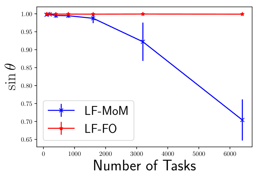
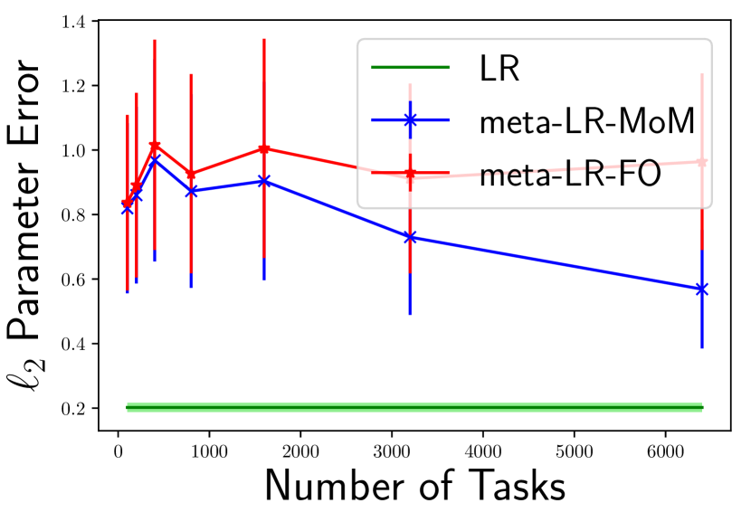
Figure 1: Left: LF-FO vs. LF-MoM estimator with error measured in the subspace angle distance $\sin\theta(\hat{\mathbf{B}},\mathbf{B})$. Right: meta-LR-FO and meta-LR-MoM vs. LR on new task with error measured on new task parameter. Here $d=100$, $r=5$, and $n_{t}=5$ while $n_{2}=2500$ as the number of tasks is varied.

As Fig. 1 demonstrates, the method-of-moments estimator is able to aggregate information across the tasks as $t$ increases to slowly improve its feature estimate, even though $n_{t}\ll d$. The loss-based approach struggles to improve its estimate of the feature matrix $\mathbf{B}$ in this regime. This accords with the extra $t$ dependence in Theorem 2 relative to Theorem 3. In this setting, we also generated a ($t+1$)st test task with $d\ll n_{2}=2500$, to test the effect of meta-learning the linear representation on generalization in a new, unseen task against a baseline which simply performs a regression on this new task in isolation. Fig. 1 also shows that meta-learned regressions perform significantly worse than simply ignoring first $t$ tasks. Theorem 4 indicates the bias from the inability to learn an accurate feature estimate of $\mathbf{B}$ overwhelms the benefits of transfer learning. In this regime $n_{2}\gg d$ so the new task can be efficiently learned in isolation. We believe this simulation represents a simple instance of the empirically observed phenomena of “negative” transfer (Wang et al., 2019).

We now turn to the more interesting use cases where meta-learning is a powerful tool. We consider a setting where $d=100$, $r=5$, and $n_{t}=25$ for varying numbers of tasks $t$. However, now we consider a new, unseen task where data is scarce: $n_{2}=25<d$.

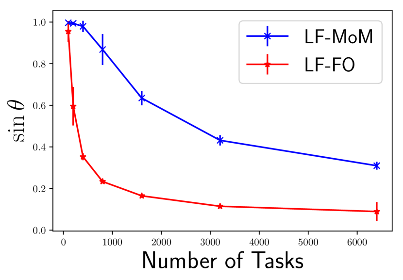
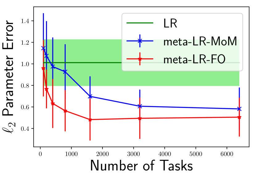
Figure 2: Left: LF-FO vs. LF-MoM estimator with error measured in the subspace angle distance $\sin\theta(\hat{\mathbf{B}},\mathbf{B})$. Right: meta-LR-FO and meta-LR-MoM vs. LR on new task with error measured on new task parameter. Here $d=100$, $r=5$, $n_{t}=25$ while $n_{2}=25$ while the number of tasks is varied.

As Fig. 2 shows, in this regime both the method-of-moments estimator and the loss-based approach can learn a non-trivial estimate of the feature representation. The benefits of transferring this representation are also evident in the improved generalization performance seen by the meta-regression procedures on the new task. Interestingly, the loss-based approach learns an accurate feature representation $\hat{\mathbf{B}}$ with significantly fewer samples then the method-of-moments estimator, in contrast to the previous experiment.

Similarly, if we consider an instance where $d=100$, $r=5$, $t=20$, and $n_{2}=50$ with varying numbers of training points $n_{t}$ per task, we see in Fig. 3 that meta-learning of representations provides significant value in a new task. Note that these numerical experiments show that as the number of tasks is fixed, but $n_{t}$ increases, the generalization ability of the meta-learned regressions significantly improves as reflected in the bound 2. As in the previous experiment, the loss-based approach is more sample-efficient then the method-of-moments estimator.

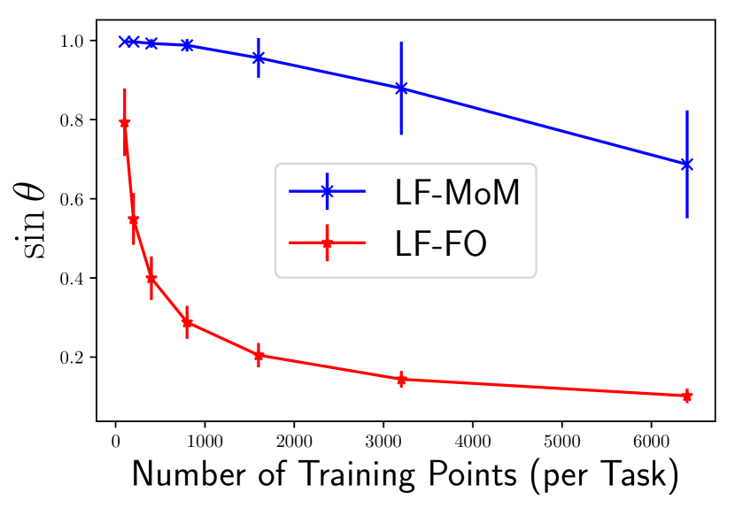
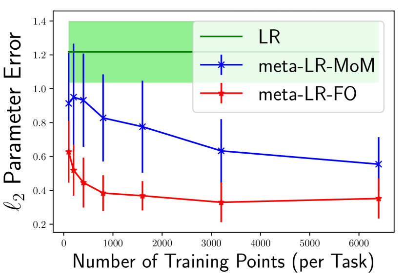
Figure 3: Left: LF-FO vs. LF-MoM estimator with error measured in the subspace angle distance $\sin\theta(\hat{\mathbf{B}},\mathbf{B})$. Right: meta-LR-FO and meta-LR-MoM vs. LR on new task with error measured on new task parameter. Here $d=100$, $r=5$, $t=20$, and $n_{2}=50$ while the number of training points per task ($n_{t}$) is varied.

7 Conclusions

In this paper we show how a shared linear representation may be efficiently learned and transferred between multiple linear regression tasks. We provide both upper and lower bounds on the sample complexity of learning this representation and for the problem of learning-to-learn. We believe our bounds capture important qualitative phenomena observed in real meta-learning applications absent from previous theoretical treatments.

8 Acknowledgements

The authors thank Niladri Chatterji for helpful discussions. This work was supported by the Army Research Office (ARO) under contract W911NF-17-1-0304 as part of the collaboration between US DOD, UK MOD and UK Engineering and Physical Research Council (EPSRC) under the Multidisciplinary University Research Initiative (MURI).

Notation and Set-up We first establish several useful pieces of notation used throughout the Appendices. We will say that a mean-zero random variable $x$ is sub-gaussian, $x\sim\text{sG}(\kappa)$, if $\mathbb{E}[\exp(\lambda x))]\leq\exp(\frac{\kappa^{2}\lambda^{2}}{2})$ for all $\lambda$. We will say that a mean-zero random variable $x$ is sub-exponential, $x\sim\text{sE}(\nu,\alpha)$, if $\mathbb{E}[\exp(\lambda x)]\leq\exp(\frac{\nu^{2}\lambda^{2}}{2})$ for all $|{\lambda}|\leq\frac{1}{\alpha}$. We will say that a mean-zero random vector is sub-gaussian, $\mathbf{x}\sim\text{sG}(\kappa)$, if $\forall\mathbf{v}\in\mathbb{R}^{p}$, $\mathbb{E}[\exp(\mathbf{v}^{\top}\mathbf{x})]\leq\exp(\frac{\kappa^{2}\|\mathbf{v}\|_{2}^{2}}{2})$. A standard Chernoff argument shows that if $x\sim\text{sE}(\nu,\alpha)$ then $\mathbb{P}[|{x}|\geq t]\leq 2\exp(-\frac{1}{2}\min(\frac{t^{2}}{\nu^{2}},\frac{t}{\alpha}))$. Throughout we will use $c,C$ to refer to universal constants that may change from line to line.

Appendix A Proofs for Section 1

Here we provide a formal statement of Theorem 1.

Theorem 6 (Formal statement of Theorem 1).

Suppose we are first given $n_{1}$ total samples from 1 which satisfy Assumption 1 and $\mathbf{x}_{i}\sim\mathcal{N}(0,\mathbf{I}_{d})$, with an equal number of samples from each task, which collectively satisfy Assumption 2. Then, we are presented $n_{2}$ samples also from 1, satisfying Assumption 1, but from a $t+1$st task which satisfies $\|{\bm{\alpha}_{t+1}}\|^{2}\leq O(1)$. If the $n_{1}$ samples are used in Algorithm 1 to learn a feature representation $\hat{\mathbf{B}}$, which is used in Algorithm 2 along with the $n_{2}$ samples to learn $\hat{\bm{\alpha}}$, and $n_{1}\gtrsim\mathrm{polylog}(d,n_{1})\frac{\bar{\kappa}dr}{\nu}$, $n_{2}\gtrsim r\log n_{2}$, the excess prediction error on a new datapoint drawn from the covariate distribution, is,

$$\mathbb{E}_{\mathbf{x}_{\star}}[\langle\mathbf{x}_{\star},\hat{\mathbf{B}}\hat{\bm{\alpha}}-\mathbf{B}\bm{\alpha}_{t+1}\rangle^{2}]\leq\tilde{O}\left(\frac{\bar{\kappa}dr}{\nu n_{1}}+\frac{r}{n_{2}}\right),$$

with probability at least $1-O(n_{1}^{-100}+n_{2}^{-100})$.

Proof.

Note that $\mathbb{E}_{\mathbf{x}_{\star}}[\langle\mathbf{x}_{\star},\hat{\mathbf{B}}\hat{\bm{\alpha}}-\mathbf{B}\bm{\alpha}_{t+1}\rangle^{2}]=\|{\hat{\mathbf{B}}\hat{\bm{\alpha}}-\mathbf{B}\bm{\alpha}_{t+1}}\|^{2}$. Combining Theorem 3, Theorem 4 and applying a union bound then gives the result. ∎

Note that in order to achieve the formulation in Theorem 1, we make the simplifying assumption that the training tasks are well-conditioned in the sense that $\bar{\kappa}\leq\kappa\leq O(1)$ and $\nu\geq\Omega(\frac{1}{r}$)—which is consistent with the normalization in Assumption 2. Such a setting is for example achieved (w.h.p.) if each $\bm{\alpha}_{t}\sim\mathcal{N}(0,\frac{1}{\sqrt{r}}\mathbf{\Sigma})$ where $\sigma_{1}(\mathbf{\Sigma})/\sigma_{r}(\mathbf{\Sigma})\leq O(1)$.

Appendix B Proofs for Section 3.2

Analyzing the performance of the method-of-moments estimator requires two steps. First, we show that the estimator $(1/n)\cdot\sum_{i=1}^{n}y_{i}^{2}\mathbf{x}_{i}\mathbf{x}_{i}^{\top}$ converges to its mean in spectral norm, up to error fluctuations $\tilde{O}(\sqrt{\frac{dr}{n}})$. Showing this requires adapting tools from the theory of matrix concentration. Second, a standard application of the Davis-Kahan $\sin\theta$ theorem shows that top-r PCA applied to this noisy matrix, $(1/n)\cdot\sum_{i=1}^{n}y_{i}^{2}\mathbf{x}_{i}\mathbf{x}_{i}^{\top}$, can extract a subspace $\hat{\mathbf{B}}$ close to the true column space of $\mathbf{B}$ up to a small error. Throughout this section we let $\bar{\mathbf{\Gamma}}=\frac{1}{n}\sum_{i=1}^{n}\bar{\mathbf{\Gamma}}_{i}$ with $\bar{\mathbf{\Gamma}}_{i}=\mathbf{B}\bm{\alpha}_{t(i)}\bm{\alpha}_{t(i)}^{\top}\mathbf{B}^{\top}$. We also let $\bar{\mathbf{\Lambda}}=\frac{1}{n}\sum_{i=1}^{n}\bm{\alpha}_{t(i)}\bm{\alpha}_{t(i)}^{\top}$ be the empirically observed task matrix. Note that under Assumption 2, we have that $\bar{\mathbf{\Gamma}}$ and $\bar{\mathbf{\Lambda}}$ behave identically since $\mathbf{B}$ has orthonormal columns we have that $\mathrm{tr}(\bar{\mathbf{\Gamma}})=\mathrm{tr}(\bar{\mathbf{\Lambda}})$ and $\sigma_{r}(\bar{\mathbf{\Gamma}})=\sigma_{r}(\bar{\mathbf{\Lambda}})$. Furthermore throughout this section we use $\tilde{\kappa}$ and $\tilde{\nu}$ to refer to the average condition number and $r$-th singular value of the empirically observed task matrix $\bar{\mathbf{\Lambda}}$ – since all our results hold in generality for this matrix. Note that under the uniform task observation model the task parameters of $\bar{\mathbf{\Lambda}}$ and the population task matrix $\frac{\mathbf{A}^{\top}\mathbf{A}}{t}$ are equal.

We first present our main theorem which shows our method-of-moments estimator can recover the true subspace $\mathbf{B}$ up to small error.

Proof of Theorem 3.

The proof follows by combining the Davis-Kahan sin $\theta$ theorem with our main concentration result for the matrix $\frac{1}{n}\sum_{i=1}^{n}y_{i}^{2}\mathbf{x}_{i}^{\top}\mathbf{x}_{i}-\mathbb{E}[\frac{1}{n}\sum_{i=1}^{n}y_{i}^{2}\mathbf{x}_{i}^{\top}\mathbf{x}_{i}]$. First note that $\mathbb{E}[\frac{1}{n}\sum_{i=1}^{n}y_{i}^{2}\mathbf{x}_{i}^{\top}\mathbf{x}_{i}]=(2\bar{\mathbf{\Gamma}}+(1+\mathrm{tr}(\bar{\mathbf{\Gamma}}))\mathbf{I}_{d}$ by Lemma 2 and define $\frac{1}{n}\sum_{i=1}^{n}y_{i}^{2}\mathbf{x}_{i}^{\top}\mathbf{x}_{i}-\mathbb{E}[\frac{1}{n}\sum_{i=1}^{n}y_{i}^{2}\mathbf{x}_{i}^{\top}\mathbf{x}_{i}]=\mathbf{E}$. Note that under the conditions of the result for $n\geq cd$ we have that $\|{\mathbf{E}}\|\leq\tilde{O}(\sqrt{\frac{d\tilde{\kappa}r\tilde{\nu}}{n}})$ by Theorem 7 for large-enough $c$ due to the SNR normalization; so again by taking sufficiently large $c$ such that $n\geq c\cdot\mathrm{polylog}(d,n)\tilde{\kappa}rd/\tilde{\nu}$ we can ensure that $\|{\mathbf{E}}\|\leq\delta\leq 2\tilde{\nu}$ for as small $\delta$ as we choose with the requisite probability. Since $\|{\mathbf{E}}\|\leq\delta$ we have that $\sigma_{r+1}(y_{i}^{2}\mathbf{x}_{i}\mathbf{x}_{i}^{\top})-\sigma_{r+1}((2\bar{\mathbf{\Gamma}}+(1+\mathrm{tr}(\bar{\mathbf{\Gamma}}))\mathbf{I}_{d})\leq\delta$ and since $\bar{\mathbf{\Gamma}}$ is rank $r$, $\sigma_{r}((2\bar{\mathbf{\Gamma}}+(1+\mathrm{tr}(\bar{\mathbf{\Gamma}}))\mathbf{I}_{d})-\sigma_{r+1}((2\bar{\mathbf{\Gamma}}+(1+\mathrm{tr}(\bar{\mathbf{\Gamma}}))\mathbf{I}_{d})=2\sigma_{r}(\bar{\mathbf{\Gamma}})$. Hence, applying the Davis-Kahan $\sin\theta$ theorem shows that,

$$\|{\hat{\mathbf{B}}_{\perp}^{\top}\mathbf{B}}\|\leq\frac{\|{\hat{\mathbf{B}}_{\perp}^{\top}\mathbf{E}\mathbf{B}}\|}{2\sigma_{r}(\bar{\mathbf{\Lambda}})-\delta}\leq\frac{\|{\mathbf{E}}\|}{2\sigma_{r}(\bar{\mathbf{\Lambda}})-\delta}\leq\frac{\|{\mathbf{E}}\|}{\tilde{\nu}}\leq\tilde{O}\left(\sqrt{\frac{1}{\tilde{\nu}}\frac{d\tilde{\kappa}r}{n}}\right),$$

where the final inequalities follows by taking $c$ large enough to ensure $\delta\leq\tilde{\nu}$ and Theorem 7.

∎

We now present our main result which proves the concentration of the estimator,

Theorem 7.

Suppose the $n$ data samples $(\mathbf{x}_{i},y_{i})$ are generated from the model in (12) and that Assumptions 1, LABEL: and 2 hold with $\mathbf{x}_{i}\sim\mathcal{N}(0,1)$ i.i.d. Then if $n\gtrsim c$ for sufficiently large $c$,

$$\|{\frac{1}{n}\sum_{i=1}^{n}y_{i}^{2}\mathbf{x}_{i}\mathbf{x}_{i}^{\top}-(2\bar{\mathbf{\Gamma}}+(1+\mathrm{tr}(\bar{\mathbf{\Gamma}}))\mathbf{I}_{d}))}\|\leq$$

$$\log^{3}n\cdot\log^{3}d\cdot O\left(\sqrt{\frac{d\tilde{\kappa}r\tilde{\nu}}{n}}+\frac{d}{n}\right),$$

with probability at least $1-O(n^{-100})$.

Proof.

Note that the mean of $\frac{1}{n}\sum_{i=1}^{n}y_{i}^{2}\mathbf{x}_{i}\mathbf{x}_{i}^{\top}$ is $2\bar{\mathbf{\Gamma}}+(1+\mathrm{tr}(\bar{\mathbf{\Gamma}}))\mathbf{I}_{d})$ by Lemma 2. Then using the fact that $y_{i}=\mathbf{x}_{i}^{\top}\mathbf{B}\bm{\alpha}_{t(i)}+\epsilon_{i}$, we can write down the error decomposition for the estimator into signal and noise terms,

$$\frac{1}{n}\sum_{i=1}^{n}y_{i}^{2}\mathbf{x}_{i}\mathbf{x}_{i}^{\top}-(2\bar{\mathbf{\Gamma}}+(1+\mathrm{tr}(\bar{\mathbf{\Gamma}}))\mathbf{I}_{d}=\frac{1}{n}\sum_{i=1}^{n}(\mathbf{x}_{i}\mathbf{B}\bm{\alpha}_{t(i)})^{2}\mathbf{x}_{i}\mathbf{x}_{i}^{\top}-(2\bar{\mathbf{\Gamma}}+\mathrm{tr}(\bar{\mathbf{\Gamma}}))\mathbf{I}_{d}+$$

$$\frac{1}{n}\sum_{i=1}^{n}2\epsilon_{i}\mathbf{x}_{i}\mathbf{B}\bm{\alpha}_{t(i)}\mathbf{x}_{i}\mathbf{x}_{i}^{\top}+\frac{1}{n}\sum_{i=1}^{n}\epsilon_{i}^{2}\mathbf{x}_{i}\mathbf{x}_{i}^{\top}-\mathbf{I}_{d}.$$

We proceed to control the fluctuations of each term in spectral norm individually using tools from matrix concentration. Applying Lemma 3, Lemma 4, Lemma 5, the triangle inequality and a union bound shows the desired quantity is upper bounded as,

$$\log^{3}n\cdot\log^{3}d\cdot O\left(\sqrt{\frac{d\max(1,\mathrm{tr}(\bar{\mathbf{\Gamma}}),\mathrm{tr}(\bar{\mathbf{\Gamma}})\max_{i}\|{\bm{\beta}_{i}}\|^{2})}{n}}+\frac{d\max(1,\max_{i}\|{\bm{\beta}_{i}}\|,\max_{i}\|{\bm{\beta}_{i}}\|^{2})}{n}\right).$$

Finally, using Assumption 2 and the fact that $\mathrm{tr}{\bar{\mathbf{\Gamma}}}=\mathrm{tr}{\bar{\mathbf{\Lambda}}}$ and the fact $\|{\bm{\beta}_{i}}\|=\|{\bm{\alpha}_{i}}\|$, simplifies the result to the theorem statement. Note that since $\|{\bm{\alpha}_{i}}\|=\Theta(1)$ for all $i$ we have that, $\mathrm{tr}(\bar{\mathbf{\Gamma}})=\Theta(1)$ so the SNR normalization guarantees the leading noise term satisfies $1\leq O(\mathrm{tr}(\bar{\mathbf{\Gamma}}))$. ∎

We begin by computing the mean of the estimator.

Lemma 2.

Suppose the $n$ data samples $(\mathbf{x}_{i},y_{i})$ are generated from the model in (1) and that Assumptions 1, LABEL: and 2 hold. Then,

$$\mathbb{E}[\frac{1}{n}\sum_{i=1}^{n}y_{i}^{2}\mathbf{x}_{i}\mathbf{x}_{i}^{\top}]=2\bar{\mathbf{\Gamma}}+(1+\mathrm{tr}(\bar{\mathbf{\Gamma}}))\mathbf{I}_{d}$$

where $\bar{\mathbf{\Gamma}}=\frac{1}{n}\sum_{i=1}^{n}\bar{\mathbf{\Gamma}}_{i}$ with $\mathbf{\Gamma}_{i}=\mathbf{B}\bm{\alpha}_{t(i)}\bm{\alpha}_{t(i)}^{\top}\mathbf{B}^{\top}$.

Proof.

Since $\epsilon_{i}$ is mean-zero, using the definition of $y_{i}$ we immediately obtain,

$$\mathbb{E}[\frac{1}{n}\sum_{i=1}^{n}y_{i}^{2}\mathbf{x}_{i}\mathbf{x}_{i}^{\top}]=\mathbf{I}_{d}+\mathbb{E}[\frac{1}{n}\sum_{i=1}^{n}\mathbf{x}_{i}^{\top}\mathbf{\Gamma}_{i}\mathbf{x}_{i}\mathbf{x}_{i}\mathbf{x}_{i}^{\top}]=\mathbf{I}_{d}+\mathbb{E}[\mathbf{x}^{\top}\bar{\mathbf{\Gamma}}\mathbf{x}\mathbf{x}\mathbf{x}^{\top}],$$

for $\mathbf{x}\sim\mathcal{N}(0,\mathbf{I}_{d})$. Using the eigendecomposition of $\bar{\mathbf{\Gamma}}$ we have that $\mathbb{E}[\mathbf{x}^{\top}\bar{\mathbf{\Lambda}}\mathbf{x}\mathbf{x}\mathbf{x}^{\top}]=\sum_{i=1}^{r}\sigma_{i}\mathbb{E}[(\mathbf{x}^{\top}\mathbf{v}_{i})^{2}\mathbf{x}\mathbf{x}^{\top}]$. Due to the isotropy of the Gaussian distribution, it suffices to compute $\mathbb{E}[(\mathbf{x}^{\top}\mathbf{e}_{1})^{2}\mathbf{x}\mathbf{x}^{\top}]$ and rotate the result back to $\mathbf{v}_{i}$. In particular we have that,

$$(\mathbb{E}[(\mathbf{x}^{\top}\mathbf{e}_{1})^{2}\mathbf{x}\mathbf{x}^{\top}])_{ij}=\begin{cases}0\quad i\neq j\\ 1\quad i=j\neq 1\\ 3\quad i=j=1\\ \end{cases}\implies\mathbb{E}[(\mathbf{x}^{\top}\mathbf{e}_{1})^{2}\mathbf{x}\mathbf{x}^{\top}]=2\mathbf{e}_{1}\mathbf{e}_{1}+\mathbf{I}_{d}\implies$$

$$\implies\mathbb{E}[(\mathbf{x}^{\top}\mathbf{v}_{i})^{2}\mathbf{x}\mathbf{x}^{\top}]=2\mathbf{v}_{i}\mathbf{v}_{i}+\mathbf{I}_{d}\implies\mathbf{E}[\mathbf{x}^{\top}\bar{\mathbf{\Gamma}}\mathbf{x}\mathbf{x}\mathbf{x}^{\top}]=2\bar{\mathbf{\Gamma}}+\mathrm{tr}(\bar{\mathbf{\Gamma}})\mathbf{I}_{d},$$

from which the conclusion follows. ∎

We start by controlling the fluctuations of the final noise term (which has identity mean).

Lemma 3.

Suppose the $n$ data samples $(\mathbf{x}_{i},y_{i})$ are generated from the model in (1) and that Assumptions 1, LABEL: and 2 hold. Then for $n\geq c$ for sufficiently large $c$,

$$\|{\frac{1}{n}\sum_{i=1}^{n}\epsilon_{i}^{2}\mathbf{x}_{i}\mathbf{x}_{i}^{\top}-\mathbf{I}_{d}}\|\leq O\left(\log^{2}n\left(\sqrt{\frac{d}{n}}+\frac{d}{n}\right)\right).$$

with probability at least $1-O(n^{-100})$.

Proof.

We first decompose the expression as,

$$\|{\frac{1}{n}\sum_{i=1}^{n}\epsilon_{i}^{2}\mathbf{x}_{i}\mathbf{x}_{i}^{\top}-\mathbf{I}_{d}}\|\leq\|{\frac{1}{n}\sum_{i=1}^{n}\epsilon_{i}^{2}\mathbf{x}_{i}\mathbf{x}_{i}^{\top}-\frac{1}{n}\sum_{i=1}^{n}\epsilon_{i}^{2}\mathbf{I}_{d}}\|+\|{\frac{1}{n}\sum_{i=1}^{n}\epsilon_{i}^{2}\mathbf{I}_{d}-\mathbf{I}_{d}}\|$$

We begin by controlling the second term. By a sub-exponential tail bound we have that $\mathbb{P}[|{\frac{1}{n}\sum_{i=1}^{n}\epsilon_{i}^{2}-1}|\geq t]\leq 2\exp(-Cn\min(t^{2}/8^{2},t/8))$, since $\epsilon_{i}^{2}$ is $\text{sE}(8,8)$ by Lemma 26. Letting $t=c\sqrt{\log(\frac{1}{\delta})/n}$ for sufficiently large $c$, and assuming $n\gtrsim\log(\frac{1}{\delta})$, implies $|{\frac{1}{n}\sum_{i=1}^{n}\epsilon_{i}^{2}-1}|\leq O(\sqrt{\frac{\log(1/\delta)}{n}})$ with probability at least $1-2\delta$. Hence $\|{\frac{1}{n}\sum_{i=1}^{n}\epsilon_{i}^{2}\mathbf{I}_{d}-\mathbf{I}_{d}}\|\leq O(\sqrt{\frac{\log(1/\delta)}{n}})$ on this event.

Now we apply Lemma 27 with $a_{i}=\epsilon_{i}$ to control the first term. Using the properties of sub-Gaussian maxima we can conclude that $\mathbb{P}[\max_{i}|{\epsilon}|_{i}\geq t]\leq 2n\exp(-t^{2}/2)$; taking $t=4\sqrt{\log n}+c\sqrt{\log(1/\delta)}$ for sufficiently large $c$ implies that $\max_{i}|{\epsilon_{i}}|\leq O(\sqrt{\log n})+O(\sqrt{\log(1/\delta)})$ with probability at least $1-\delta$. In the setting of Lemma 27, conditionally on $\epsilon_{i}$, $K=\max_{i}|\epsilon_{i}|$ and $\mathbf{\Sigma}=\mathbf{I}_{d}$ so taking $t=c\sqrt{\log(1/\delta)}$ for sufficiently large $c$ implies that $\|{\frac{1}{n}\sum_{i=1}^{n}\epsilon_{i}^{2}\mathbf{x}_{i}\mathbf{x}_{i}^{\top}-\frac{1}{n}\sum_{i=1}^{n}\epsilon_{i}^{2}\mathbf{I}_{d}}\|\leq K\cdot O(\sqrt{d/n}+\sqrt{\log(1/\delta)/n}+\frac{d}{n}+\frac{\log(1/\delta)}{n})$ with probability at least $1-2\delta$ conditionally on $\epsilon_{i}$. Conditioning on the event that $\max_{i}|{\epsilon_{i}}|\leq O(\sqrt{\log n})+O(\sqrt{\log(1/\delta)})$ to conclude the argument finally shows that,

$$\|{\frac{1}{n}\sum_{i=1}^{n}\epsilon_{i}^{2}\mathbf{x}_{i}\mathbf{x}_{i}^{\top}-\mathbf{I}_{d}}\|\leq O(\log n+\log(1/\delta))\cdot O(\sqrt{\frac{d}{n}}+\sqrt{\frac{\log(1/\delta)}{n}}+\frac{d}{n}+\frac{\log(1/\delta)}{n})+O(\sqrt{\frac{\log(1/\delta)}{n}}),$$

with probability at least $1-5\delta$. Selecting $\delta=n^{-100}$ implies that $\|{\frac{1}{n}\sum_{i=1}^{n}\epsilon_{i}^{2}\mathbf{x}_{i}\mathbf{x}_{i}^{\top}-\mathbf{I}_{d}}\|\leq O\left(\log^{2}n\left(\sqrt{\frac{d}{n}}+\frac{d}{n}\right)\right)$, with probability at least $1-O(n^{-100})$. ∎

We now proceed to controlling the fluctuations of the second noise term (which is mean-zero). Our main technical tool is Lemma 31.

Lemma 4.

Suppose the $n$ data samples $(\mathbf{x}_{i},y_{i})$ are generated from the model in (1) and that Assumptions 1, LABEL: and 2 hold. Then,

$$\|{\frac{1}{n}\sum_{i=1}^{n}2\epsilon_{i}\mathbf{x}_{i}^{\top}\mathbf{B}\bm{\alpha}_{t(i)}\mathbf{x}_{i}\mathbf{x}_{i}^{\top}}\|\leq O((\log n+\log d)\left(\sqrt{\frac{d\mathrm{tr}(\bar{\mathbf{\Gamma}})}{n}}+\frac{d\max_{i}\|{\bm{\beta}_{i}}\|(\log^{2}(n)+\log^{2}(d))}{n}\right).$$

with probability at least $1-O((nd)^{-100})$.

Proof.

To apply the truncated version of the matrix Bernstein inequality (in the form of Lemma 31) we need to set an appropriate truncation level $R$, for which need control on the norms of $Z_{i}=\|{2\epsilon_{i}\mathbf{x}_{i}^{\top}\mathbf{B}\bm{\alpha}_{t(i)}\mathbf{x}_{i}\mathbf{x}_{i}^{\top}}\|=2|{\epsilon_{i}}|\|{\mathbf{x}_{i}}\|^{2}|{\mathbf{x}_{i}^{\top}\mathbf{B}\bm{\alpha}_{t(i)}}|$. Using sub-gaussian, and sub-exponential tail bounds we have that $|{\epsilon_{i}}|\leq O(1+\sqrt{\log(1/\delta)})$, $\|{\mathbf{x}_{i}}\|^{2}\leq O(d+\max(\sqrt{d\log(1/\delta)},\log(1/\delta)))=O(d+\sqrt{d}\log(1/\delta))$, and $|{\mathbf{x}_{i}^{\top}\mathbf{B}\bm{\alpha}_{t(i)}}|\leq O(\|{\bm{\beta}_{i}}\|(1+\sqrt{\log(1/\delta)})$ each with probability at least $1-\delta$. Accordingly with probability at least $1-3\delta$ we have that $\|{Z_{i}}\|\leq O(\|{\bm{\beta}_{i}}\|d(1+\log^{2}(1/\delta)))$. We can rearrange this statement to conclude that $\mathbb{P}[\|{Z_{i}}\|\geq c_{1}\|{\bm{\beta}_{i}}\|d+t]\leq 3\exp(-c_{2}(\frac{t}{\|{\bm{\beta}_{i}}\|d})^{1/2})$ for some $c_{1},c_{2}$. Define a truncation level $R=c_{1}\max_{i}\|{\bm{\beta}_{i}}\|d+K\max_{i}\|{\bm{\beta}_{i}}\|d$ for some $K$ to be chosen later. We can also use the aforementioned tail bound to control $\|{\mathbb{E}[Z_{i}]-\mathbb{E}[Z_{i}^{\prime}]}\|\leq\mathbb{E}[Z_{i}\mathbbm{1}{[}\|{Z_{i}}\|\geq\alpha]]\leq\int_{K\|{\bm{\beta}_{i}}\|d}^{\infty}3\exp(-c_{2}(\frac{t}{\|{\bm{\beta}_{i}}\|d})^{1/2})\leq O((1+\sqrt{K})\exp(-c\sqrt{K})\max_{i}\|{\bm{\beta}_{i}}\|d)=\Delta$.

Next we must compute an upper bound for the matrix variance term

$$\|{\sum_{i=1}^{n}\mathbb{E}[\epsilon_{i}^{2}(\bm{\alpha}_{i}^{\top}\mathbf{B}^{\top}\mathbf{x}_{i})^{2}\|{\mathbf{x}_{i}}\|^{2}\mathbf{x}_{i}\mathbf{x}_{i}^{\top}]}\|=\|{\sum_{i=1}^{n}\mathbb{E}[(\bm{\alpha}_{i}^{\top}\mathbf{B}^{\top}\mathbf{x})^{2}\|{\mathbf{x}}\|^{2}\mathbf{x}\mathbf{x}^{\top}]}\|=n\|{\mathbb{E}[\mathbf{x}^{\top}\bar{\mathbf{\Gamma}}\mathbf{x}\|{\mathbf{x}}\|^{2}\mathbf{x}\mathbf{x}^{\top}]}\|=n\|{\sum_{i=1}^{r}\sigma_{i}\mathbb{E}[(\mathbf{v}_{i}^{\top}\mathbf{x})^{2}\|{\mathbf{x}}\|^{2}\mathbf{x}\mathbf{x}^{\top}]}\|$$

, taking an expectation over $\epsilon_{i}$ in the first equality, and diagonalizing $\bar{\mathbf{\Gamma}}$. As before due to isotropy of the Gaussian it suffices to compute the expectation with $\mathbf{v}_{i}=\mathbf{e}_{1}$ and rotate the result back to $\mathbf{v}_{i}$. Before computing the term we note that for a standard normal gaussian random variable $g\sim\mathcal{N}(0,1)$ we have that $\mathbb{E}[g^{6}]=15$, $\mathbb{E}[g^{4}]=3$, $\mathbb{E}[g^{2}]=1$. Then by simple combinatorics we find that,

$$(\mathbb{E}[x_{1}^{2}(\sum_{a=1}^{n}x_{a}^{2})\mathbf{x}\mathbf{x}^{\top}])_{ij}=\begin{cases}0\quad i\neq j\neq 1\\ 0\quad i=1\neq j\\ 2\cdot 3\cdot 1+(d-2)\cdot 1\quad i=j\neq 1\\ 15+3(d-1)\quad i=j=1\\ \end{cases}\implies$$

$$\mathbb{E}[(\mathbf{x}^{\top}\mathbf{e}_{1})^{2}\|{\mathbf{x}}\|^{2}\mathbf{x}\mathbf{x}^{\top}]=(2d+8)\mathbf{e}_{1}\mathbf{e}_{1}^{\top}+(d+4)\mathbf{I}_{d}$$

$$\implies\|{\sum_{i=1}^{n}\mathbb{E}[\epsilon_{i}^{2}(\bm{\alpha}_{i}^{\top}\mathbf{B}^{\top}\mathbf{x}_{i})^{2}\|{\mathbf{x}_{i}}\|^{2}\mathbf{x}_{i}\mathbf{x}_{i}^{\top}]}\|\leq n(d+4)\|{\bar{\mathbf{\Gamma}}+\mathrm{tr}(\bar{\mathbf{\Gamma}})\mathbf{I}_{d}}\|\leq 10nd(\mathrm{tr}(\bar{\mathbf{\Gamma}}))=\sigma^{2}.$$

Finally, we can assemble the previous two computations to conclude the result with appropriate choices of $R$ (parametrized through $K$) and $t$ by combining with Lemma 31. Before beginning recall by definition we have that $\mathrm{tr}(\bar{\mathbf{\Gamma}})=\frac{1}{n}\max_{i}\|{\bm{\beta}_{i}}\|^{2}$. Let us choose $\sqrt{K}=\frac{c_{3}}{c}(\log(n)+\log(d))$ for some sufficiently large $c_{3}$. In this case, we can choose $c_{3}$ such that $\Delta\leq O((\log n+\log d)\frac{\max_{i}\|{\bm{\beta}_{i}}\|d}{n^{10}d^{10}})\leq O(\frac{\sqrt{\mathrm{tr}(\bar{\mathbf{\Gamma}})}}{n^{8}d^{8}})$, since $\sqrt{\mathrm{tr}(\bar{\mathbf{\Gamma}})}\geq\frac{1}{\sqrt{n}}\max_{i}\|{\bm{\beta}_{i}}\|$. Similarly, our choice of truncation level becomes $R=O((\log^{2}(n)+\log^{2}(d))\max_{i}\|{\bm{\beta}_{i}}\|d)$. At this point we now choose $t=c_{4}(\log n+\log d)\max(\sigma/\sqrt{n},R/n)$ for sufficiently large $c_{4}$. For large enough $c_{4}$ we can guarantee that $t\geq 2\Delta\implies t-\Delta\geq\frac{t}{2}$.

Hence combining these results together and applying Lemma 31 we can provide the following upper bound on the desired quantity,

$$\mathbb{P}[\|{\frac{1}{n}\sum_{i=1}^{n}2\epsilon_{i}\mathbf{x}_{i}^{\top}\mathbf{B}\bm{\alpha}_{t(i)}\mathbf{x}_{i}\mathbf{x}_{i}^{\top}}\|\geq t]\leq O(d\exp(-c\cdot c_{4}(\log n+\log d))+O(n\sqrt{K}\exp(-c_{3}(\log n+\log d))\leq O((nd)^{-100}),$$

by taking $c_{3}$ and $c_{4}$ sufficiently large, with $t=O((\log n+\log d)\left(\sqrt{\frac{d\mathrm{tr}(\bar{\mathbf{\Gamma}})}{n}}+\frac{d\max_{i}\|{\bm{\beta}_{i}}\|(\log^{2}(n)+\log^{2}(d))}{n}\right)$. ∎

Finally we turn to controlling the fluctuations of the primary signal term around its mean using a similar argument to the previous term.

Lemma 5.

Suppose the $n$ data samples $(\mathbf{x}_{i},y_{i})$ are generated from the model in (1) and that Assumptions 1, LABEL: and 2 hold. Then

$$\|{\frac{1}{n}\sum_{i=1}^{n}(\mathbf{x}_{i}\mathbf{B}\bm{\alpha}_{t(i)})^{2}\mathbf{x}_{i}\mathbf{x}_{i}^{\top}-(2\bar{\mathbf{\Gamma}}+\mathrm{tr}(\bar{\mathbf{\Gamma}})\mathbf{I}_{d})}\|\leq$$

$$O((\log n+\log d)\left(\sqrt{\frac{d\mathrm{tr}(\bar{\mathbf{\Gamma}})\max_{i}\|{\bm{\beta}_{i}}\|^{2}}{n}}+\frac{d\max_{i}\|{\bm{\beta}_{i}}\|^{2}(\log^{2}(n)+\log^{2}(d))}{n}\right),$$

with probability at least $1-O((nd)^{-100})$.

Proof.

The proof is similar to the proof of Lemma 4 and uses Lemma 31. We begin by controlling the norms of $Z_{i}=(\mathbf{x}_{i}^{\top}\mathbf{B}\bm{\alpha}_{t(i)})^{2}\mathbf{x}_{i}\mathbf{x}_{i}^{\top}$. $\|{Z_{i}}\|=\|{\mathbf{x}_{i}}\|^{2}(\mathbf{x}_{i}^{\top}\mathbf{B}\bm{\alpha}_{t(i)})^{2}$. Using Gaussian and sub-exponential tail bounds we have that, $\|{\mathbf{x}_{i}}\|^{2}\leq O(d+\sqrt{d}\log(1/\delta))$ and $(\mathbf{x}_{i}^{\top}\mathbf{B}\bm{\alpha}_{t(i)})^{2}\leq O(\|{\bm{\beta}_{i}}\|^{2}(1+\log(1/\delta)))$ each with probability at least $1-\delta$. Hence with probability at least $1-2\delta$ we find that $\|{Z_{i}}\|\leq O(d\|{\bm{\beta}_{i}}\|^{2}(1+\log^{2}(1/\delta))$.

We can rearrange this statement to conclude that $\mathbb{P}[\|{Z_{i}}\|\geq c_{1}\|{\bm{\beta}_{i}}\|^{2}d+t]\leq 2\exp(-c_{2}(\frac{t}{\|{\bm{\beta}_{i}}\|^{2}d})^{1/2})$ for some $c_{1},c_{2}$. Define a truncation level $R=c_{1}\max_{i}\|{\bm{\beta}_{i}}\|^{2}d+K\max_{i}\|{\bm{\beta}_{i}}\|^{2}d$ for some $K$ to be chosen later. We can use the aforementioned tail bound to control $\|{\mathbb{E}[Z_{i}]-\mathbb{E}[Z_{i}^{\prime}]}\|\leq\mathbb{E}[Z_{i}\mathbbm{1}{[}\|{Z_{i}}\|\geq\alpha]]\leq\int_{K\|{\bm{\beta}_{i}}\|^{2}d}^{\infty}2\exp(-c_{2}(\frac{t}{\|{\bm{\beta}_{i}}\|^{2}d})^{1/2})\leq O((1+\sqrt{K})\exp(-c\sqrt{K})\max_{i}\|{\bm{\beta}_{i}}\|^{2}d)=\Delta$.

Next we must compute an upper bound the matrix variance term

$$\|{\sum_{i=1}^{n}\mathbb{E}[(\bm{\alpha}_{i}^{\top}\mathbf{B}^{\top}\mathbf{x}_{i})^{4}\|{\mathbf{x}_{i}}\|^{2}\mathbf{x}_{i}\mathbf{x}_{i}^{\top}]}\|=\|{\sum_{i=1}^{n}\mathbb{E}[(\bm{\beta}_{i}^{\top}\mathbf{x})^{4}\|{\mathbf{x}}\|^{2}\mathbf{x}\mathbf{x}^{\top}]}\|.$$

As before due to isotropy of the Gaussian it suffices to compute each expectation assuming $\bm{\beta}_{i}\propto\mathbf{e}_{1}$ and rotate the result back to $\bm{\beta}_{i}$. Before computing the term we note that for a standard normal gaussian random variable $g\sim\mathcal{N}(0,1)$ we have that $\mathbb{E}[g^{8}]=105$, $\mathbb{E}[g^{6}]=15$, $\mathbb{E}[g^{4}]=3$, $\mathbb{E}[g^{2}]=1$. Then by simple combinatorics we find that,

$$(\mathbb{E}[(\mathbf{x}^{\top}\mathbf{e}_{1})^{4}(\sum_{a=1}^{n}x_{a}^{2})\mathbf{x}\mathbf{x}^{\top}])_{ij}=\begin{cases}0\quad i\neq j\neq 1\\ 0\quad i=1\neq j\\ 15+3\cdot 3+(d-2)\cdot 3\quad i=j\neq 1\\ 105+15(d-1)\quad i=j=1\\ \end{cases}\implies$$

$$\mathbb{E}[(\mathbf{x}^{\top}\bm{\beta}_{i})^{4}\|{\mathbf{x}}\|^{2}\mathbf{x}\mathbf{x}^{\top}]=(2d+75)\mathbf{e}_{1}\mathbf{e}_{1}^{\top}+(3d+15)\mathbf{I}_{d}$$

$$\implies\|{\sum_{i=1}^{n}\mathbb{E}[(\bm{\alpha}_{i}^{\top}\mathbf{B}^{\top}\mathbf{x}_{i})^{4}\|{\mathbf{x}_{i}}\|^{2}\mathbf{x}_{i}\mathbf{x}_{i}^{\top}]}\|\leq O(d)\|{\sum_{i}^{n}\|{\bm{\beta}_{i}}\|^{4}(\bm{\beta}_{i}\bm{\beta}_{i}^{\top}+\mathbf{I}_{d})}\|\leq O(d\sum_{i=1}^{n}\|{\bm{\beta}_{i}}\|_{2}^{4})\leq$$

$$O(dn\max_{i}\|{\bm{\beta}_{i}}\|^{2}\mathrm{tr}(\bar{\mathbf{\Gamma}}))=\sigma^{2}.$$

Finally, we can assemble the previous two computations to conclude the result with appropriate choices of $R$ (parametrized through $K$) and $t$ by combining with Lemma 31. Before beginning recall by definition we have that $\mathrm{tr}{\bar{\mathbf{\Gamma}}}\geq\frac{1}{n}\max_{i}\|{\bm{\beta}_{i}}\|^{2}$. Let us choose $\sqrt{K}=\frac{c_{3}}{c}(\log(n)+\log(d))$ for some sufficiently large $c_{3}$. In this case, we can choose $c_{3}$ such that $\Delta\leq O((\log n+\log d)\frac{\max_{i}\|{\bm{\beta}_{i}}\|^{2}d}{n^{10}d^{10}})\leq O(\frac{\sqrt{\mathrm{tr}(\bar{\mathbf{\Gamma}})}\max_{i}\|{\bm{\beta}_{i}}\|}{n^{7}d^{7}})$, since $\sqrt{\mathrm{tr}(\bar{\mathbf{\Gamma}})}\geq\frac{1}{\sqrt{n}}\max_{i}\|{\bm{\beta}_{i}}\|$. Similarly, our choice of truncation level becomes $R=O((\log^{2}(n)+\log^{2}(d))\max_{i}\|{\bm{\beta}_{i}}\|^{2}d)$. At this point we now choose $t=c_{4}(\log n+\log d)\max(\sigma/\sqrt{n},R/n)$ for sufficiently large $c_{4}$. For large enough $c_{4}$ we can guarantee that $t\geq 2\Delta\implies t-\Delta\geq\frac{t}{2}$.

Hence combining these results together and applying Lemma 31 we can provide the following upper bound on the desired quantity:

$$\mathbb{P}[\|{\frac{1}{n}\sum_{i=1}^{n}(\mathbf{x}_{i}\mathbf{B}\bm{\alpha}_{t(i)})^{2}\mathbf{x}_{i}\mathbf{x}_{i}^{\top}-(2\bar{\mathbf{\Gamma}}+\mathrm{tr}(\bar{\mathbf{\Gamma}})\mathbf{I}_{d})}\|\geq t]$$

$$\leq O(d\exp(-c\cdot c_{4}(\log n+\log d))+O(n\sqrt{K}\exp(-c_{3}(\log n+\log d))$$

$$\leq O((nd)^{-100}),$$

by taking $c_{3}$ and $c_{4}$ sufficiently large, with

$$t=O((\log n+\log d)\left(\sqrt{\frac{d\mathrm{tr}(\bar{\mathbf{\Gamma}})\max_{i}\|{\bm{\beta}_{i}}\|^{2}}{n}}+\frac{d\max_{i}\|{\bm{\beta}_{i}}\|^{2}(\log^{2}(n)+\log^{2}(d))}{n}\right).$$

. ∎

Appendix C Proofs for Section 3.1

In our landscape analysis we consider a setting with $t$ tasks and we observe a datapoint from each of the $t$ tasks uniformly at random at each iteration. Formally, we define the matrix we are trying to recover as

$$\mathbf{M}_{\star}=(\bm{\alpha}_{1},\ldots,\bm{\alpha}_{t})^{\top}\mathbf{B}^{\top}\underbrace{=}_{\text{SVD}}\mathbf{X}^{\star}\mathbf{D}^{\star}(\mathbf{Y}{\star})^{\top}\in\mathbb{R}^{t\times d},$$ (8)

with $\mathbf{U}^{\star}=\mathbf{X}^{\star}(\mathbf{D}^{\star})^{1/2}$, and $(\mathbf{D}^{\star})^{1/2}(\mathbf{Y}^{\star})^{\top}=(\mathbf{V}^{\star})^{\top}$, from which we obtain the observations:

$$y_{i}=\langle\mathbf{e}_{t(i)}\mathbf{x}_{i}^{\top},\mathbf{M}_{\star}\rangle+\sigma\cdot\epsilon_{i},$$ (9)

where we sample tasks uniformly $t(i)\sim\{1,\ldots,t\}$ and $\mathbf{x}_{i}$ is a sub-gaussian random vector. Note that $\mathbf{M}^{\star}$ is a rank-$r$ matrix, $\mathbf{U}^{\star}\in\mathbb{R}^{t\times r}$, and $\mathbf{V}^{\star}\in\mathbb{R}^{d\times r}$. In this section, we denote $\tilde{d}=\max\{t,d\}$ and let $\sigma^{\star}_{1},\sigma^{\star}_{r}$ be the $1$-st and $r$-th eigenvalue of matrix $\mathbf{M}^{\star}$. We denote $\kappa^{\star}=\sigma^{\star}_{1}/\sigma^{\star}_{r}$ as its condition number. Note that as $\mathbf{B}$ is an orthonormal matrix we have that $\mathbf{M}^{\star}(\mathbf{M}^{\star})^{\top}=t\cdot\mathbf{A}^{\top}\mathbf{A}/t$ from which it follows that $(\sigma^{\star}_{1})^{2}=t\cdot\sigma_{1}(\mathbf{A}^{\top}\mathbf{A}/t)\leq t\bar{\kappa}\nu\leq O(t)$ by the normalization on $\|{\bm{\alpha}_{i}}\|$. Similarly $(\sigma^{\star}_{r})^{2}=t\sigma_{r}(\mathbf{A}^{\top}\mathbf{A}/t)\geq t\nu$. So it follows that $\sigma^{\star}_{1}\leq\sqrt{t\kappa\nu}$, $\sigma^{\star}_{r}\geq\sqrt{t\nu}$ and $\kappa^{\star}\leq\sqrt{\kappa}$. We use this to simplify the preconditions and the statement of the incoherence ball in the main although we work in full generality throughout the Appendix.

We now present the proof of our main result.

Proof of Theorem 2.

Under the conditions of the theorem note that by Theorem 8 we have that,

$$\|{\mathbf{U}\mathbf{V}^{\top}-\mathbf{M}^{\star}}\|_{F}\leq O\left(\sigma\sqrt{t\frac{\max\{t,d\}r\log n}{n}}\right),$$

for $n\geq\mathrm{polylog}(n,d,t)C\mu^{2}r^{4}\max\{t,d\}(\kappa^{\star})^{4}$. First recall by Lemma 17 the incoherence parameter can in fact be shown to be $\mu=O(\bar{\kappa})$ under our assumptions which gives the precondition on the sample complexity due to the task diversity assumption and normalization. To finally convert this bound to a guarantee on the subspace angle we directly apply Lemma 16 once again noting the task diversity assumption. Lastly note that as $\mathbf{B}$ is orthonormal we have that $\sigma^{\star}_{1}\leq\sqrt{t\kappa\nu}$, $\sigma^{\star}_{r}\geq\sqrt{t\nu}$ and $\kappa^{\star}\leq\sqrt{\kappa}$ as previously argued and $\sigma=1$ under the conditions of the result. ∎

C.1 Geometric Arguments for Landscape Analysis

Our arguments here are generally applicable to various matrix sensing/completion problems so we define some generic notation:

$$f(\mathbf{U},\mathbf{V})=\frac{2}{n}\sum_{i=1}^{n}(\langle\mathbf{A}_{i},\mathbf{U}\mathbf{V}^{\top}\rangle-\sqrt{t}y_{i})^{2}+\frac{1}{2}\|{\mathbf{U}^{\top}\mathbf{U}-\mathbf{V}^{\top}\mathbf{V}}\|_{\text{F}}^{2},$$ (10)

where $\mathbf{A}_{i}=\sqrt{t}\mathbf{e}_{t(i)}\mathbf{x}_{i}^{\top}$. We work under the following constraint set for large constant $C_{0}$:

$$\mathcal{W}=\{~{}(\mathbf{U},\mathbf{V})~{}|~{}\max_{i\in[t]}\|{\mathbf{e}_{i}^{\top}\mathbf{U}}\|^{2}\leq\frac{C_{0}\mu r\sigma^{\star}_{1}}{t},\quad\|{\mathbf{U}}\|^{2}\leq C_{0}\sigma^{\star}_{1},\quad\|{\mathbf{V}}\|^{2}\leq C_{0}\sigma^{\star}_{1}~{}\}.$$ (11)

We renormalize the statistical model for convenience simply for the purposes of the proof throughout Appendix C the remainder of as:

$$y_{i}=\langle\mathbf{A}_{i},\mathbf{M}^{\star}\rangle+n_{i},$$ (12)

where $n_{i}\sim\sqrt{t}\sigma\cdot\epsilon_{i}$ and where $\epsilon_{i}$ is a sub-gaussian random vector with parameter 1 (note this is because we have scaled $\mathbf{A}_{i}$ up by a factor of $\sqrt{t}$). $\mathbf{M}^{\star}$ is rank $r$, and we let $\mathbf{X}$ be the left singular vector of $\mathbf{M}^{\star}$, and assume $\mathbf{X}$ is $\mu$-incoherent; i.e., $\max_{i}\|{\mathbf{e}_{i}^{\top}\mathbf{X}}\|^{2}\leq\mu r/t$.

We now reformulate the objective (denoting $\mathbf{M}=\mathbf{U}\mathbf{V}^{\top}$) as

$$f(\mathbf{U},\mathbf{V})=2(\mathbf{M}-\mathbf{M}^{\star}):\mathcal{H}_{0}:(\mathbf{M}-\mathbf{M}^{\star})+\frac{1}{2}\|{\mathbf{U}^{\top}\mathbf{U}-\mathbf{V}^{\top}\mathbf{V}}\|_{\text{F}}^{2}+Q(\mathbf{U}),$$ (13)

where $\mathbf{M}:\mathcal{H}_{0}:\mathbf{M}=\frac{1}{n}\sum_{i=1}^{n}\langle\mathbf{A}_{i},\mathbf{M}\rangle^{2}$ and $\mathbf{E}[\mathbf{M}:\mathcal{H}_{0}:\mathbf{M}]=\|{\mathbf{M}}\|_{\text{F}}^{2}$ and $Q$ is a regularization term:

$$Q(\mathbf{U},\mathbf{V})=\frac{2}{n}\sum_{i=1}^{n}[(\langle\mathbf{M}-\mathbf{M}^{\star},\mathbf{A}_{i}\rangle-n_{i})^{2}-(\langle\mathbf{M}-\mathbf{M}^{\star},\mathbf{A}_{i}\rangle)^{2}].$$ (14)

In this section, we denote $\tilde{d}=\max\{t,d\}$ and let $\sigma^{\star}_{1},\sigma^{\star}_{r}$ be the $1$-st and $r$-th eigenvalue of matrix $\mathbf{M}^{\star}$. We denote $\kappa^{\star}=\sigma^{\star}_{1}/\sigma^{\star}_{r}$ as its condition number.

The high-level idea of the analysis uses ideas from Ge et al. [2017]. The overall strategy is to argue that if we are currently not located at local minimum in the landscape we can certify this by inspecting the gradient or Hessian of $f(\mathbf{U},\mathbf{V})$ to exhibit a direction of local improvement $\Delta$ to decrease the function value of $f$. Intuitively this direction brings us close to the true underlying $(\mathbf{U}^{\star},\mathbf{V}^{\star})$.

We now establish some useful definitions and notation for the following analysis

C.1.1 Definitions and Notation

Definition 1.

Suppose $\mathbf{M}^{\star}$ is the optimal solution with SVD is $\mathbf{X}^{\star}\mathbf{D}^{\star}\mathbf{Y}^{\star}{}^{\top}$. Let $\mathbf{U}^{\star}=\mathbf{X}^{\star}(\mathbf{D}^{\star})^{\frac{1}{2}}$, $\mathbf{V}^{\star}=\mathbf{Y}^{\star}(\mathbf{D}^{\star})^{\frac{1}{2}}$. Let $\mathbf{M}=\mathbf{U}\mathbf{V}^{\top}$ be the current point in the landscape. We reduce the problem of studying an asymmetric matrix objective to the symmetric case using the following notational transformations:

$$\mathbf{W}=\begin{pmatrix}\mathbf{U}\\ \mathbf{V}\end{pmatrix},\mathbf{W}^{\star}=\begin{pmatrix}\mathbf{U}^{\star}\\ \mathbf{V}^{\star}\end{pmatrix},\mathbf{N}=\mathbf{W}\mathbf{W}^{\top},\mathbf{N}^{\star}=\mathbf{W}^{\star}\mathbf{W}^{\star}{}^{\top}$$ (15)

We will also transform the Hessian operators to operate on $(t+d)\times r$ matrices. In particular, define the Hessians $\mathcal{H}_{1},\mathcal{G}$ such that for all $\mathbf{W}$ we have:

$$\mathbf{N}:\mathcal{H}_{1}:\mathbf{N} =\mathbf{M}:\mathcal{H}_{0}:\mathbf{M}$$

$$\mathbf{N}:\mathcal{G}:\mathbf{N} =\|{\mathbf{U}^{\top}\mathbf{U}-\mathbf{V}^{\top}\mathbf{V}}\|_{F}^{2}.$$

Now, letting $Q(\mathbf{W})=Q(\mathbf{U},\mathbf{V})$, we can rewrite the objective function $f(\mathbf{W})$ as

$$\frac{1}{2}\left[(\mathbf{N}-\mathbf{N}^{\star}):4\mathcal{H}_{1}:(\mathbf{N}-\mathbf{N}^{\star})+\mathbf{N}:\mathcal{G}:\mathbf{N}\right]+Q(\mathbf{W}).$$ (16)

We now introduce the definition of local alignment of two matrices.

Definition 2.

Given matrices $\mathbf{W},\mathbf{W}^{\star}\in\mathbb{R}^{d\times r}$, define their difference $\Delta=\mathbf{W}-\mathbf{W}^{\star}\mathbf{R}^{\star}$, where $\mathbf{R}^{\star}\in\mathbb{R}^{r\times r}$ is chosen as $\mathbf{R}^{\star}=\mathop{\rm argmin}_{\mathbf{Z}^{\top}\mathbf{Z}=\mathbf{Z}\mathbf{Z}^{\top}=\mathbf{I}}\|\mathbf{W}-\mathbf{W}^{\star}\mathbf{Z}\|_{F}^{2}.$

Note that this definition tries to “align” $\mathbf{U}$ and $\mathbf{U}^{\star}$ before taking their difference, and therefore is invariant under rotations. In particular, this definition has the nice property that as long as $\mathbf{N}=\mathbf{W}\mathbf{W}^{\top}$ is close to $\mathbf{N}^{\star}=\mathbf{W}^{\star}(\mathbf{W}^{\star})^{\top}$ in Frobenius norm, the corresponding $\Delta$ between them is also small (see Lemma 8).

C.1.2 Proofs for Landscape Analysis

With these definitions in hand we can now proceed to the heart of the landscape analysis. Since $\mathbf{W}^{\star}$ has rotation invariance, in the following section we always choose $\mathbf{W}^{\star}$ so that it aligns with the corresponding $\mathbf{W}$ according to Definition 2.

We first restate a useful result from Ge et al. [2017],

Lemma 6 ([Ge et al., 2017, Lemma 16]).

For the objective (16), let $\Delta,\mathbf{N},\mathbf{N}^{\star}$ be defined as in Definition 1, Definition 2. Then, for any $\mathbf{W}\in\mathbf{R}^{(t+d)\times r}$, we have

$$\Delta:\nabla^{2}f(\mathbf{W}):\Delta\leq \Delta\Delta^{\top}:\mathcal{H}:\Delta\Delta^{\top}-3(\mathbf{N}-\mathbf{N}^{\star}):\mathcal{H}:(\mathbf{N}-\mathbf{N}^{\star})$$

$$+4\langle\nabla f(\mathbf{W}),\Delta\rangle+[\Delta:\nabla^{2}Q(\mathbf{W}):\Delta-4\langle\nabla Q(\mathbf{W}),\Delta\rangle],$$ (17)

where $\mathcal{H}=4\mathcal{H}_{1}+\mathcal{G}$. Further, if $\mathcal{H}_{0}$ satisfies $\mathbf{M}:\mathcal{H}_{0}:\mathbf{M}\in(1\pm\delta)\|\mathbf{M}\|_{F}^{2}$ for some matrix $\mathbf{M}=\mathbf{U}\mathbf{V}^{\top}$, let $\mathbf{W}$ and $\mathbf{N}$ be defined as in (15), then $\mathbf{N}:\mathcal{H}:\mathbf{N}\in(1\pm 2\delta)\|\mathbf{N}\|_{F}^{2}$.

With this result we show a key result which shows that with enough samples all stationary points in the incoherence ball $\mathcal{W}$ that are not close to $\mathbf{W}^{\star}$ have a direction of negative curvature.

Lemma 7.

If Assumption 1 holds, then when the number of samples $n\geq C\mathrm{polylog}(d,n,t)\mu^{2}r^{4}\max\{t,d\}(\kappa^{\star})^{4}$ for a sufficiently large constant $C$, with probability at least $1-1/\mathrm{poly}(d)$, all stationary points $\mathbf{W}\in\text{int}(\mathcal{W})$ satisfy:

$$\Delta\Delta^{\top}:\mathcal{H}:\Delta\Delta^{\top}-3(\mathbf{N}-\mathbf{N}^{\star}):\mathcal{H}:(\mathbf{N}-\mathbf{N}^{\star})\leq-0.1\|{\mathbf{N}-\mathbf{N}^{\star}}\|_{\text{F}}^{2}.$$

Proof.

We divide the proof into two cases according to the norm of $\Delta$ and use different concentration inequalities in each case. In this proof, we denote $\Delta=(\Delta_{\mathbf{U}}^{\top},\Delta_{\mathbf{V}}^{\top})^{\top}$, clearly, we have $\|{\Delta_{\mathbf{U}}}\|_{\text{F}}\leq\|{\Delta}\|_{\text{F}}$ and $\|{\Delta_{\mathbf{V}}}\|_{\text{F}}\leq\|{\Delta}\|_{\text{F}}$.

Case 1: $\|{\Delta}\|_{\text{F}}^{2}\leq\sigma^{\star}_{r}/1000$. In this case, $\|{\Delta_{\mathbf{U}}}\|_{\text{F}}^{2}\leq\|{\Delta}\|_{\text{F}}^{2}\leq\sigma^{\star}_{r}/1000$ and $\|{\Delta_{\mathbf{V}}}\|_{\text{F}}^{2}\leq\|{\Delta}\|_{\text{F}}^{2}\leq\sigma^{\star}_{r}/1000$. By (19), we have

$$\Delta\Delta^{\top}:\mathcal{H}:\Delta\Delta^{\top}\leq\|{\Delta\Delta^{\top}}\|_{\text{F}}^{2}+0.004\sigma^{\star}_{r}\|{\Delta_{\mathbf{V}}}\|_{\text{F}}^{2}\leq 0.005\sigma^{\star}_{r}\|{\Delta}\|_{\text{F}}^{2}$$

On the other hand, denote $\mathbf{S}=\mathbf{W}^{\star}\Delta^{\top}+\Delta(\mathbf{W}^{\star})^{\top}$, by (18) and Lemma 6, we know:

$$\mathbf{S}:\mathcal{H}:\mathbf{S}\geq 0.999\|{\mathbf{S}}\|_{\text{F}}^{2}.$$

Since we choose $\mathbf{W}^{\star}$ to align with the corresponding $\mathbf{W}$ according to Definition 2, by Lemma 8.

$$\|{\mathbf{S}}\|_{\text{F}}^{2}=2(\|{\Delta^{\top}\mathbf{W}^{\star}}\|_{\text{F}}^{2}+\|{\Delta(\mathbf{W}^{\star})^{\top}}\|_{\text{F}}^{2})\geq 2\|{\Delta(\mathbf{W}^{\star})^{\top}}\|_{\text{F}}^{2}\geq 2\sigma^{\star}_{r}\|{\Delta}\|_{\text{F}}^{2}.$$

This gives:

$$\Delta\Delta^{\top}:\mathcal{H}:\Delta\Delta^{\top}-3(\mathbf{N}-\mathbf{N}^{\star}):\mathcal{H}:(\mathbf{N}-\mathbf{N}^{\star})$$

$$=\Delta\Delta^{\top}:\mathcal{H}:\Delta\Delta^{\top}-3(\mathbf{S}+\Delta\Delta^{\top}):\mathcal{H}:(\mathbf{S}+\Delta\Delta^{\top})$$

$$\leq-6\mathbf{S}:\mathcal{H}:\Delta\Delta^{\top}-3\mathbf{S}:\mathcal{H}:\mathbf{S}$$

$$\leq-\mathbf{S}:\mathcal{H}:\mathbf{S}-2\sqrt{\mathbf{S}:\mathcal{H}:\mathbf{S}}(\sqrt{\mathbf{S}:\mathcal{H}:\mathbf{S}}-3\sqrt{\Delta\Delta^{\top}:\mathcal{H}:\Delta\Delta^{\top}})$$

$$\leq-0.999\|{\mathbf{S}}\|_{\text{F}}^{2}-2\sqrt{\mathbf{S}:\mathcal{H}:\mathbf{S}}\cdot\sqrt{\sigma^{\star}_{r}}\cdot(\|{\Delta}\|_{\text{F}}-0.3\|{\Delta}\|_{\text{F}})\leq-0.999\|{\mathbf{S}}\|_{\text{F}}^{2}.$$

Finally, we know $\mathbf{N}-\mathbf{N}^{\star}=\mathbf{S}+\Delta\Delta^{\top}$, and $\|{\mathbf{S}}\|_{\text{F}}^{2}\geq 2\sigma^{\star}_{r}\|{\Delta}\|_{\text{F}}^{2}\geq 500\|{\Delta}\|_{\text{F}}^{4}=500\|{\Delta\Delta^{\top}}\|_{\text{F}}^{2}$. Therefore:

$$\|{\mathbf{N}-\mathbf{N}^{\star}}\|_{\text{F}}\leq\|{\mathbf{S}}\|_{\text{F}}+\|{\Delta\Delta^{\top}}\|_{\text{F}}\leq 2\|{\mathbf{S}}\|_{\text{F}}.$$

This gives:

$$\Delta\Delta^{\top}:\mathcal{H}:\Delta\Delta^{\top}-3(\mathbf{N}-\mathbf{N}^{\star}):\mathcal{H}:(\mathbf{N}-\mathbf{N}^{\star})\leq-0.999\|{\mathbf{S}}\|_{\text{F}}^{2}\leq-0.1\|{\mathbf{N}-\mathbf{N}^{\star}}\|_{\text{F}}^{2}.$$

Case 2: $\|{\Delta}\|_{\text{F}}^{2}\geq\sigma^{\star}_{r}/1000$, by (20), we have:

$$\frac{1}{n}\sum_{i=1}^{n}\langle\mathbf{A}_{i},\mathbf{M}-\mathbf{M}^{\star}\rangle^{2}\geq \|{\mathbf{M}-\mathbf{M}^{\star}}\|_{\text{F}}^{2}-(\sigma^{\star}_{r})^{2}/10^{6}\geq\|{\mathbf{M}-\mathbf{M}^{\star}}\|_{\text{F}}^{2}-0.001\sigma^{\star}_{r}\|{\Delta}\|_{\text{F}}^{2}.$$

This implies:

$$(\mathbf{N}-\mathbf{N}^{\star}):\mathcal{H}:(\mathbf{N}-\mathbf{N}^{\star})\geq\|{\mathbf{N}-\mathbf{N}^{\star}}\|_{\text{F}}^{2}-0.004\sigma^{\star}_{r}\|{\Delta}\|_{\text{F}}^{2}.$$

Then by (19), we have:

$$\Delta\Delta^{\top}:\mathcal{H}:\Delta\Delta^{\top}-3(\mathbf{N}-\mathbf{N}^{\star}):\mathcal{H}:(\mathbf{N}-\mathbf{N}^{\star})$$

$$\leq \|{\Delta\Delta^{\top}}\|_{\text{F}}^{2}+0.004\sigma^{\star}_{r}\|{\Delta}\|_{\text{F}}^{2}-3(\|{\mathbf{N}-\mathbf{N}^{\star}}\|_{\text{F}}^{2}-0.004\sigma^{\star}_{r}\|{\Delta}\|_{\text{F}}^{2})$$

$$\leq -\|{\mathbf{N}-\mathbf{N}^{\star}}\|_{\text{F}}^{2}+0.016\sigma^{\star}_{r}\|{\Delta}\|_{\text{F}}^{2}\leq-0.1\|{\mathbf{N}-\mathbf{N}^{\star}}\|_{\text{F}}^{2},$$

where the last step follows by applying Lemma 8. This finishes the proof. ∎

With this key structural lemma in hand, we now present the main technical result for the section which characterizes the effect of the additive noise $n_{i}$ on the landscape.

Theorem 8.

If Assumption 1 holds, when the number of samples $n\geq C\mathrm{polylog}(n,d,t)\mu^{2}r^{4}\max\{t,d\}(\kappa^{\star})^{4}$ for sufficiently large constant $C$, with probability at least $1-1/\mathrm{poly}(d)$, we have that any local minimum $(\mathbf{U},\mathbf{V})\in\text{int}(\mathcal{W})$ of the objective (10) satisfies:

$$\|{\mathbf{U}\mathbf{V}^{\top}-\mathbf{M}^{\star}}\|_{F}\leq O\left(\sigma\sqrt{\frac{t\max\{t,d\}r\log n}{n}}\right).$$

Proof.

By Lemma 7, we know

$$\Delta\Delta^{\top}:\mathcal{H}:\Delta\Delta^{\top}-3(\mathbf{N}-\mathbf{N}^{\star}):\mathcal{H}:(\mathbf{N}-\mathbf{N}^{\star})\leq-0.1\|\mathbf{N}-\mathbf{N}^{\star}\|_{F}^{2}.$$

In order to use Lemma 6, we bound the contribution from the noise term $Q$. Recall (14):

$$Q(\mathbf{W})= -\frac{4}{n}\sum_{i=1}^{n}(\langle\mathbf{M}-\mathbf{M}^{\star},\mathbf{A}_{i}\rangle n_{i})+\frac{2}{n}\sum_{i=1}^{n}(n_{i})^{2}$$

$$\langle\nabla Q(\mathbf{W}),\Delta\rangle= -\frac{4}{n}\sum_{i=1}^{n}(\langle\mathbf{U}\Delta_{\mathbf{V}}^{\top}+\Delta_{\mathbf{U}}\mathbf{V}^{\top},\mathbf{A}_{i}\rangle n_{i})$$

$$\Delta:\nabla^{2}Q(\mathbf{W}):\Delta= -\frac{8}{n}\sum_{i=1}^{n}(\langle\Delta_{\mathbf{U}}\Delta_{\mathbf{V}}^{\top},\mathbf{A}_{i}\rangle n_{i}).$$

Let $\mathbf{B}_{i}$ be the $(d_{1}+d_{2})\times(d_{1}+d_{2})$ matrix whose diagonal blocks are 0, and off diagonal blocks are equal to $\mathbf{A}_{i}$ and $\mathbf{A}_{i}^{\top}$ respectively. Then we have

$$[\Delta:\nabla^{2}Q(\mathbf{W}):\Delta-4\langle\nabla Q(\mathbf{W}),\Delta\rangle]$$

$$=-\frac{8}{n}\sum_{i=1}^{n}(\langle\Delta_{\mathbf{U}}\Delta_{\mathbf{V}}^{\top},\mathbf{A}_{i}\rangle n_{i})+\frac{16}{n}\sum_{i=1}^{n}(\langle\mathbf{U}\Delta_{\mathbf{V}}^{\top}+\Delta_{\mathbf{U}}\mathbf{V}^{\top},\mathbf{A}_{i}\rangle n_{i})$$

$$=\frac{24}{n}\sum_{i=1}^{n}(\langle\Delta_{\mathbf{U}}\Delta_{\mathbf{V}}^{\top},\mathbf{A}_{i}\rangle n_{i})+\frac{16}{n}\sum_{i=1}^{n}(\langle\mathbf{U}^{\star}\Delta_{\mathbf{V}}^{\top}+\Delta_{\mathbf{U}}(\mathbf{V}^{\star})^{\top},\mathbf{A}_{i}\rangle n_{i})$$

Now we can use Lemma 15 again to bound the noise terms:

$$|\frac{24}{n}\sum_{i=1}^{n}(\langle\Delta_{\mathbf{U}}\Delta_{\mathbf{V}}^{\top},\mathbf{A}_{i}\rangle n_{i})| \leq O\left(\sigma\sqrt{\frac{t\max\{t,d\}r\log n}{n}}\right)\sqrt{\|{\Delta_{\mathbf{U}}\Delta_{\mathbf{V}}^{\top}}\|_{\text{F}}^{2}+0.001\sigma^{\star}_{r}\|{\Delta_{\mathbf{V}}}\|_{\text{F}}^{2}}$$

$$|\frac{16}{n}\sum_{i=1}^{n}(\langle\mathbf{U}^{\star}\Delta_{\mathbf{V}}^{\top}+\Delta_{\mathbf{U}}(\mathbf{V}^{\star})^{\top},\mathbf{A}_{i}\rangle n_{i})| \leq O\left(\sigma\sqrt{\frac{t\max\{t,d\}r\log n}{n}}\right)\|{\mathbf{U}^{\star}\Delta_{\mathbf{V}}^{\top}+\Delta_{\mathbf{U}}(\mathbf{V}^{\star})^{\top}}\|_{F}.$$

On the one hand, by Lemma 8, we have:

$$\|{\Delta_{\mathbf{U}}\Delta_{\mathbf{V}}^{\top}}\|_{\text{F}}^{2}+0.001\sigma^{\star}_{r}\|{\Delta_{\mathbf{V}}}\|_{\text{F}}^{2}\leq\|{\Delta\Delta^{\top}}\|_{\text{F}}^{2}+0.001\sigma^{\star}_{r}\|{\Delta}\|_{\text{F}}^{2}\leq 3\|{\mathbf{N}-\mathbf{N}^{\star}}\|_{\text{F}}^{2}.$$

On the other hand, again by Lemma 8, we have:

$$\|{\mathbf{U}^{\star}\Delta_{\mathbf{V}}^{\top}+\Delta_{\mathbf{U}}(\mathbf{V}^{\star})^{\top}}\|^{2}_{F}\leq\|{\mathbf{W}^{\star}\Delta^{\top}+\Delta(\mathbf{W}^{\star})^{\top}}\|^{2}_{F}=2[\|{\mathbf{W}^{\star}\Delta^{\top}}\|_{\text{F}}^{2}+\|{\Delta^{\top}\mathbf{W}^{\star}}\|_{\text{F}}^{2}]\leq 10\|{\mathbf{N}-\mathbf{N}^{\star}}\|_{\text{F}}^{2}.$$

In sum, we have:

$$[\Delta:\nabla^{2}Q(\mathbf{W}):\Delta-4\langle\nabla Q(\mathbf{W}),\Delta\rangle]\leq O\left(\sigma\sqrt{\frac{t\max\{t,d\}r\log n}{n}}\right)\|{\mathbf{N}-\mathbf{N}^{\star}}\|_{\text{F}}.$$

Therefore, by Lemma 6, the Hessian at $\Delta$ direction is equal to:

$$\Delta:\nabla^{2}f(\mathbf{W}):\Delta\leq -0.1\|{\mathbf{N}-\mathbf{N}^{\star}}\|_{F}^{2}+O(\sigma\sqrt{\frac{t\max\{t,d\}r\log n}{n}})\|{\mathbf{N}-\mathbf{N}^{\star}}\|_{\text{F}}.$$

When the point further satisfies the second-order optimality condition we have

$$\|{\mathbf{N}-\mathbf{N}^{\star}}\|_{F}\leq O\left(\sigma\sqrt{\frac{t\max\{t,d\}r\log n}{n}}\right).$$

In particular, $\mathbf{M}-\mathbf{M}^{\star}$ is a submatrix of $\mathbf{N}-\mathbf{N}^{\star}$, so $\|{\mathbf{M}-\mathbf{M}^{\star}}\|_{F}\leq O(\sigma\sqrt{\frac{t\max\{t,d\}r\log n}{n}})$. ∎

C.2 Linear Algebra Lemmas

We collect together several useful linear algebra lemmas.

Lemma 8.

Given matrices $\mathbf{W},\mathbf{W}^{\star}\in\mathbb{R}^{d\times r}$, let $\mathbf{N}=\mathbf{W}\mathbf{W}^{\top}$ and $\mathbf{N}^{\star}=\mathbf{W}^{\star}(\mathbf{W}^{\star})^{\top}$, and let $\Delta,\mathbf{R}^{\star}$ be defined as in Definition 2, and let $\tilde{\mathbf{W}}^{\star}=\mathbf{W}^{\star}\mathbf{R}^{\star}$then we have the followings properties:

1. $\mathbf{W}(\tilde{\mathbf{W}}^{\star})^{\top}$ is a symmetric p.s.d. matrix;

2. $\|\Delta\Delta^{\top}\|_{F}^{2}\leq 2\|\mathbf{N}-\mathbf{N}^{\star}\|_{F}^{2}$;

3. $\sigma^{\star}_{r}\|\Delta\|_{F}^{2}\leq\|{\Delta(\tilde{\mathbf{W}}^{\star})^{\top}}\|_{\text{F}}^{2}\leq\frac{1}{2(\sqrt{2}-1)}\|\mathbf{N}-\mathbf{N}^{\star}\|_{F}^{2}$.

4. $\|{\Delta^{\top}\tilde{\mathbf{W}}^{\star}}\|_{\text{F}}^{2}\leq\|\mathbf{N}-\mathbf{N}^{\star}\|_{F}^{2}$

Proof.

Statement 1 is in the proof of Ge et al. [2017, Lemma 6]. Statement 2 is by Ge et al. [2017, Lemma 6]. Statement 3 & 4 follow by Lemma 9. ∎

Lemma 9.

Let $\mathbf{U}$ and $\mathbf{Y}$ be $d\times r$ matrices such that $\mathbf{U}^{\top}\mathbf{Y}=\mathbf{Y}^{\top}\mathbf{U}$ is a p.s.d. matrix. Then,

$$\sigma_{\min}(\mathbf{U}^{\top}\mathbf{U})\|{\mathbf{U}-\mathbf{Y}}\|_{\text{F}}^{2}\leq\|{(\mathbf{U}-\mathbf{Y})\mathbf{U}^{\top}}\|_{\text{F}}^{2}\leq \frac{1}{2(\sqrt{2}-1)}\|{\mathbf{U}\mathbf{U}^{\top}-\mathbf{Y}\mathbf{Y}^{\top}}\|_{\text{F}}^{2}$$

$$\|{(\mathbf{U}-\mathbf{Y})^{\top}\mathbf{U}}\|_{\text{F}}^{2}\leq \|{\mathbf{U}\mathbf{U}^{\top}-\mathbf{Y}\mathbf{Y}^{\top}}\|_{\text{F}}.$$

Proof.

For the first statement, the left inequality is immediate, so we only need to prove right inequality. To prove this, we let $\Delta=\mathbf{U}-\mathbf{Y}$, and expand:

$$\|{\mathbf{U}\mathbf{U}^{\top}-\mathbf{Y}\mathbf{Y}^{\top}}\|_{F}^{2}= \|{\mathbf{U}\Delta^{\top}+\Delta\mathbf{U}^{\top}-\Delta\Delta^{\top}}\|_{F}^{2}$$

$$=\mathrm{tr}(2\mathbf{U}^{\top}\mathbf{U}\Delta^{\top}\Delta+(\Delta^{\top}\Delta)^{2}+2(\mathbf{U}^{\top}\Delta)^{2}-4\mathbf{U}^{\top}\Delta\Delta^{\top}\Delta)$$

$$=\mathrm{tr}((4-2\sqrt{2})\mathbf{U}^{\top}(\mathbf{U}-\Delta)\Delta^{\top}\Delta+(\Delta^{\top}\Delta-\sqrt{2}\mathbf{U}^{\top}\Delta)^{2}+2(\sqrt{2}-1)\mathbf{U}^{\top}\mathbf{U}\Delta^{\top}\Delta)$$

$$\geq\mathrm{tr}((4-2\sqrt{2})\mathbf{U}^{\top}\mathbf{Y}\Delta^{\top}\Delta+2(\sqrt{2}-1)\mathbf{U}^{\top}\mathbf{U}\Delta^{\top}\Delta)\geq 2(\sqrt{2}-1)\|{\mathbf{U}\Delta^{\top}}\|_{\text{F}}^{2}.$$

The last inequality follows since $\mathbf{U}^{\top}\mathbf{Y}$ is a p.s.d. matrix. For the second statement, again, we have:

$$\|{\mathbf{U}\mathbf{U}^{\top}-\mathbf{Y}\mathbf{Y}^{\top}}\|_{F}^{2} =\|{\mathbf{U}\Delta^{\top}+\Delta\mathbf{U}^{\top}-\Delta\Delta^{\top}}\|_{F}^{2}$$

$$=\mathrm{tr}(2\mathbf{U}^{\top}\mathbf{U}\Delta^{\top}\Delta+(\Delta^{\top}\Delta)^{2}+2(\mathbf{U}^{\top}\Delta)^{2}-4\mathbf{U}^{\top}\Delta\Delta^{\top}\Delta)$$

$$=\mathrm{tr}(2\mathbf{U}^{\top}(\mathbf{U}-\Delta)\Delta^{\top}\Delta+(\Delta^{\top}\Delta-\mathbf{U}^{\top}\Delta)^{2}+(\mathbf{U}^{\top}\Delta)^{2})$$

$$\geq\mathrm{tr}(2\mathbf{U}^{\top}\mathbf{Y}\Delta^{\top}\Delta+(\mathbf{U}^{\top}\Delta)^{2})\geq\|{\mathbf{U}^{\top}\Delta}\|_{\text{F}}^{2},$$

where the last inequality follows since $\mathbf{U}^{\top}\Delta=\Delta^{\top}\mathbf{U}$. ∎

C.3 Concentration Lemmas

We need to show three concentration-style results for the landscape analysis. The first is an RIP condition for over matrices in the linear space $\mathcal{T}=\{\mathbf{U}_{\star}\mathbf{X}^{\top}+\mathbf{Y}\mathbf{V}_{\star}^{\top}|\mathbf{X}\in\mathbb{R}^{t\times r},\mathbf{Y}\in\mathbb{R}^{d\times r}\}$ using matrix concentration. The second and third are coarse concentration results that exploit the rank $r$ structure of the underlying matrix $\mathbf{M}$ and are used in the two distinct regimes where the distance to optimality can be small or large. Also note that throughout we can assume a left-sided incoherence condition on the underlying matrix of the form $\max_{i\in[t]}\|{\mathbf{e}_{i}^{\top}\mathbf{U}_{\star}}\|^{2}\leq\frac{\mu r}{t}$ due to Assumption 2.

We first present the RIP-style matrix concentration result which rests on an application of the matrix Bernstein inequality over a projected space. The proof has a similar flavor to results in Recht [2011]. First we define a projection operator on the space of matrices as $P_{\mathcal{T}}\mathbf{Z}=P_{\mathbf{U}}\mathbf{Z}+\mathbf{Z}P_{\mathbf{V}}-P_{\mathbf{U}}\mathbf{Z}P_{\mathbf{V}}$ where $P_{\mathbf{U}}$ and $P_{\mathbf{V}}$ are orthogonal projections onto the subspaces spanned by $U$ and $V$. While $P_{\mathbf{U}}$ and $P_{\mathbf{V}}$ are matrices, $P_{\mathcal{T}}$ is a linear operator mapping matrices to matrices. Intuitively we wish to show that for all $\mathbf{W}\in\mathbb{R}^{t\times d}$, that the observations matrices are approximately an isometry over the space of projected matrices w.h.p: $\frac{1}{n}\sum_{i=1}^{n}t(\langle\mathbf{e}_{t(i)}\mathbf{x}_{i}^{\top},P_{\mathcal{T}}\mathbf{W}\rangle^{2}\approx\|{P_{\mathcal{T}}\mathbf{W}}\|_{\text{F}}^{2}=\|{\mathbf{W}}\|_{\text{F}}^{2}$. Explicitly, we define the action of the operator $\mathbf{C}_{i}=\mathbf{A}_{i}\mathbf{A}_{i}^{\top}$ where $\mathbf{A}_{i}=\sqrt{t}\mathbf{x}_{i}\mathbf{e}_{j}^{\top}$ as $\mathbf{C}_{i}(\mathbf{M})=t\mathbf{x}_{i}\mathbf{e}_{j}^{\top}\langle\mathbf{e}_{j}\mathbf{x}_{i}^{\top},\mathbf{M}\rangle$.

We record a useful fact we will use in the sequel:

$$\sqrt{t}P_{\mathcal{T}}(\mathbf{x}_{i}\mathbf{e}_{j}^{\top})=P_{\mathbf{U}}\mathbf{e}_{i}\mathbf{x}_{j}^{\top}+\mathbf{e}_{i}(P_{\mathbf{V}}\mathbf{x}_{j})^{\top}-(P_{\mathbf{U}}\mathbf{e}_{i})(P_{\mathbf{V}}\mathbf{x}_{j})^{\top}\implies$$

$$\|{P_{\mathcal{T}}(\mathbf{x}_{i}\mathbf{e}_{j}^{\top}}\|_{\text{F}}^{2}=\langle P_{\mathcal{T}}(\mathbf{x}_{i}\mathbf{e}_{j}^{\top}),\mathbf{x}_{i}\mathbf{e}_{j}\rangle=\|{P_{\mathbf{U}}\mathbf{e}_{i}}\|^{2}\|{\mathbf{x}_{i}}\|^{2}+\|{\mathbf{e}_{i}}\|^{2}\|{P_{\mathbf{V}}\mathbf{x}_{i}}\|^{2}-\|{P_{\mathbf{U}}\mathbf{e}_{i}}\|^{2}\|{P_{\mathbf{V}}\mathbf{x}_{j}}\|^{2}\leq$$

$$\|{P_{\mathbf{U}}\mathbf{e}_{i}}\|^{2}\|{\mathbf{x}_{i}}\|^{2}+\|{P_{\mathbf{V}}\mathbf{x}_{i}}\|^{2},$$

where the last inequality holds almost surely.

We now present the proof of the RIP-style concentration result.

Lemma 10.

Under Assumptions 1, LABEL: and 2 and the uniform task sampling model above,

$$\|{\frac{1}{n}\sum_{i=1}^{n}P_{\mathcal{T}}\mathbf{A}_{i}\mathbf{A}_{i}^{\top}P_{\mathcal{T}}-P_{\mathcal{T}}}\|\leq(\log(ndt))\cdot O\left(\sqrt{\frac{\mu dr^{2}+tr^{2}}{n}}+\frac{(\mu dr+rt)\log(tdn)}{n}\right),$$

with probability at least $1-O(n^{-100})$, where $\mu=O(\bar{\kappa})$.

Proof.

Note that under the task assumption, Lemma 17 diversity implies incoherence of the matrix $\mathbf{U}^{\star}$ with incoherence parameter $\mu=O(\bar{\kappa})$. First, note $\mathbb{E}[\mathbf{C}_{i}(\mathbf{M})]=\mathbf{M}$ so $\mathbb{E}[\frac{1}{n}\sum_{i=1}^{n}P_{\mathcal{T}}\mathbf{A}_{i}P_{\mathcal{T}}-P_{\mathcal{T}}]=0$. To apply the truncated version of the matrix Bernstein inequality from Lemma 31 we first compute a bound on the norms of each $\mathbf{C}_{i}$ to set the truncation level $R$. Note that $\|{P_{\mathcal{T}}\mathbf{A}_{i}\mathbf{A}_{i}P_{\mathcal{T}}}\|=\|{P_{\mathcal{T}}(\mathbf{x}_{i}\mathbf{e}_{j}^{\top})}\|_{\text{F}}^{2}\leq t\cdot O((\frac{\mu r}{t}\|{\mathbf{x}_{i}}\|^{2}+\|{P_{\mathbf{V}}\mathbf{x}_{i}}\|^{2})$) using the fact the operator $\mathbf{A}_{i}$ is rank-one along with the Lemma 17 which shows task diversity implies incoherence with incoherence parameter $\bar{\kappa}$. Now exploiting Lemma 30 we have that $\|{\mathbf{x}_{i}}\|^{2}\leq O(d+\max(\sqrt{d\log(1/\delta)},\log(1/\delta)))=O(d+\sqrt{d}\log(1/\delta))$ and $\|{P_{V}\mathbf{x}_{i}}\|^{2}\leq O(r+\sqrt{r}\log(1/\delta))$ with probability at least $1-2\delta$ using sub-exponential tail bounds and a union bound. Hence $\|{P_{\mathcal{T}}\mathbf{A}_{i}P_{\mathcal{T}}}\|\leq O(\mu rd+\mu r\sqrt{d}\log(1/\delta))+tr+t\sqrt{r}\log(1/\delta))=O(\mu rd+tr+(\mu r\sqrt{d}+t\sqrt{r})\log(1/\delta))$.

We can rearrange this statement to conclude that $\mathbb{P}[\|{P_{\mathcal{T}}\mathbf{A}_{i}\mathbf{A}_{i}^{\top}P_{\mathcal{T}}}\|\geq c_{1}(\mu rd+tr)+x]\leq\exp(-c_{2}(\frac{x}{\mu r\sqrt{d}+t\sqrt{r}}))$ for some $c_{1},c_{2}$. Define a truncation level $R=c_{1}(\mu rd+rt)+K(\mu r\sqrt{d}+t\sqrt{r})$ for some $K$ to be chosen later. We can use the aforementioned tail bound to control $\|{\mathbb{E}[Z_{i}]-\mathbb{E}[Z_{i}^{\prime}]}\|\leq\mathbb{E}[Z_{i}\mathbbm{1}{[}\|{Z_{i}}\|\geq R]]\leq\int_{K(\mu r\sqrt{d}+t\sqrt{r})}^{\infty}\exp(-c_{2}(\frac{x}{\mu r\sqrt{d}+t\sqrt{r}}))\leq O(\exp(-cK)(\mu r\sqrt{d}+t\sqrt{r}))=\Delta$.

Now we consider the task of bounding the matrix variance term. The calculation is somewhat tedious but straightforward under our assumptions. We make use of the standard result that for two matrices $\mathbf{X}$ and $\mathbf{Y}$ that $\|{\mathbf{X}-\mathbf{Y}}\|\leq\max(\|{\mathbf{X}}\|,\|{\mathbf{Y}}\|)$.

It suffices to bound the operator norm $\|{\mathbf{E}[\|{P_{\mathcal{T}}\mathbf{A}_{i}}\|_{\text{F}}^{2}P_{\mathcal{T}}\mathbf{A}_{i}(P_{\mathcal{T}}\mathbf{A}_{i})^{\top}}\|$. Using the calculation from the prequel and carefully cancelling terms we can see that,

$$\|{\mathbb{E}[\|{P_{\mathcal{T}}\mathbf{A}_{i}}\|_{\text{F}}^{2}P_{\mathcal{T}}\mathbf{A}_{i}(P_{\mathcal{T}}\mathbf{A}_{i})^{\top}]}\|\leq t^{2}\|\mathbb{E}[(\|{P_{\mathbf{U}}\mathbf{e}_{i}}\|^{2}\|{\mathbf{x}_{i}}\|^{2}+\|{P_{\mathbf{V}}\mathbf{x}_{i}}\|^{2}-\|{P_{\mathbf{U}}\mathbf{e}_{i}}\|^{2}\|{P_{\mathbf{V}}\mathbf{x}_{j}}\|^{2})\cdot$$

$$(\|{P_{\mathbf{U}}\mathbf{e}_{i}}\|^{2}\mathbf{x}_{i}\mathbf{x}_{i}^{\top}+\|{P_{\mathbf{V}}\mathbf{x}}\|^{2}\mathbf{e}_{i}\mathbf{e}_{i}^{\top}-\|{P_{\mathbf{V}}\mathbf{x}_{i}}\|^{2}P_{\mathbf{U}}\mathbf{e}_{i}(P_{\mathbf{U}}\mathbf{e}_{i})^{\top}]\|$$

$$\leq t^{2}O(\|{\mathbb{E}[(\|{P_{\mathbf{U}}\mathbf{e}_{i}}\|^{2}\|{\mathbf{x}_{i}}\|^{2}\|{P_{\mathbf{U}}\mathbf{e}_{i}}\|^{2}\mathbf{x}_{i}\mathbf{x}_{i}^{\top}+(\|{P_{\mathbf{U}}\mathbf{e}_{i}}\|^{2}\|{\mathbf{x}_{i}}\|^{2}\|{P_{\mathbf{V}}\mathbf{x}_{i}}\|^{2}\mathbf{e}_{i}\mathbf{e}_{i}^{\top}}\|]+\|{P_{\mathbf{V}}\mathbf{x}_{i}}\|^{4}\mathbf{e}_{i}\mathbf{e}_{i}^{\top}).$$

We show how to calculate these leading terms as the subleading terms can be shown to be lower-order by identical calculations. First note using the fact that $\mathbb{E}[\|{P_{\mathbf{U}}\mathbf{e}_{i}}\|^{2}]\leq\frac{r}{t}\leq 1$, since $t\geq r$ by the task diversity assumption. Then $t^{2}\cdot\|{\mathbb{E}[(\|{P_{\mathbf{U}}\mathbf{e}_{i}}\|^{2}\|{\mathbf{x}_{i}}\|^{2}\|{P_{\mathbf{U}}\mathbf{e}_{i}}\|^{2}\mathbf{x}_{i}\mathbf{x}_{i}^{\top}}\|\leq\|{\mu rt\mathbb{E}[\|{\mathbf{x}_{i}}\|^{2}\mathbf{x}_{i}\mathbf{x}_{i}^{\top}]\mathbb{E}[\|{P_{\mathbf{U}}\mathbf{e}_{i}}\|^{2}]}\|\leq O(\mu r^{2}d)$ appealing to the fact $\mathbb{E}[\|{\mathbf{x}}\|^{2}\mathbf{x}\mathbf{x}^{\top}]\preceq O(\mathbf{I}_{d})$ by Lemma 28.

Similarly, we have that, $t^{2}\cdot\|{\mathbb{E}[\|{P_{\mathbf{U}}\mathbf{e}_{i}}\|^{2}\|{\mathbf{x}_{i}}\|^{2}\|{P_{\mathbf{V}}\mathbf{x}_{i}}\|^{2}\mathbf{e}_{i}\mathbf{e}_{i}^{\top}]}\|\leq\mu r\mathbb{E}[\|{\mathbf{x}_{i}}\|^{2}\|{P_{\mathbf{V}}\mathbf{x}_{i}}\|^{2}]\leq\mu r^{2}d$ using incoherence and by Lemma 28. Finally, we have that $t^{2}\cdot O(\|{\mathbb{E}[\|{P_{\mathbf{V}}\mathbf{x}_{i}}\|^{4}\mathbf{e}_{i}\mathbf{e}_{i}^{\top}}\|)\leq O(tr^{2})$. Hence we have that $\sigma^{2}=n\cdot O(\mu r^{2}d+tr^{2})$.

Finally, we can assemble the previous two computations to conclude the result with appropriate choices of $R$ (parametrized through $K$) and $x$ by combining with Lemma 31. Let us choose $K=\frac{c_{3}}{c}(\log(n)+\log(d)+\log(t))$ for some sufficiently large $c_{3}$. In this case, we can choose $c_{3}$ such that $\Delta\leq O(\frac{\mu r\sqrt{d}+t\sqrt{r}}{n^{10}d^{10}t^{10}})\leq O(\frac{\mu}{n^{10}d^{8}})$. Similarly, our choice of truncation level becomes $R=O(\mu rd+tr+(\log n+\log d+\log t)(\mu r\sqrt{d}+t\sqrt{r})$. At this point we now choose $x=c_{4}(\log n+\log d+\log t)\max(\sigma/\sqrt{n},R/n)$ for sufficiently large $c_{4}$. For large enough $c_{4}$ we can guarantee that $x\geq 2\Delta\implies x-\Delta\geq\frac{x}{2}$.

Hence combining these results together and applying Lemma 31 we can provide the following upper bound on the desired quantity:

$$\mathbb{P}[\|{\frac{1}{n}\sum_{i=1}^{n}P_{\mathcal{T}}\mathbf{A}_{i}P_{\mathcal{T}}-P_{\mathcal{T}}}\|\geq x]\leq$$

$$O(d\exp(-c\cdot c_{4}(\log n+\log d+\log t))+O(n\sqrt{K}\exp(-c_{3}(\log n+\log d+\log t))\leq O((ndt)^{-100})$$

by taking $c_{3}$ and $c_{4}$ sufficiently large, with $x=O((\log(ndt))\left(\sqrt{\frac{\mu dr^{2}+tr^{2}}{n}}+\frac{(\mu rd+tr)+(\mu r\sqrt{d}+t\sqrt{r})(\log(ndt)))}{n}\right)$. ∎

Lemma 11.

Let the covariates $\mathbf{x}_{i}$ satisfy the design conditions in Assumption 1 in the uniform task sampling model. Then for all matrices $\mathbf{M}$ matrices that are of rank $2r$, we have uniformly that,

$$|{\frac{1}{n}\sum_{i=1}^{n}\langle\mathbf{A}_{i},\mathbf{M}\rangle^{2}-\|{\mathbf{M}}\|_{\text{F}}^{2}}|\leq O\left(\sqrt{\frac{\max(t,d)r}{n}}\cdot\sqrt{t}\max_{i}\|{\mathbf{e}_{i}^{\top}\mathbf{M}}\|\|{\mathbf{M}}\|_{\text{F}}+\frac{\max(t,d)r}{n}\cdot t\max_{i}\|{\mathbf{e}_{i}^{\top}\mathbf{M}}\|^{2}\right).$$

with probability at least $1-(3000r)^{-10\max(t,d)r}$.

Proof.

Note that by rescaling it suffices to restrict attention to matrices $\mathbf{M}$ that are of rank $2r$ and have Frobenius norm $1$ (a set which we denote $\Gamma$). Applying Lemma 12, we have that,

$$|{\frac{1}{n}\sum_{i=1}^{n}t(\mathbf{e}_{t(i)}^{\top}\mathbf{M}\mathbf{x}_{i})^{2}-\|{\mathbf{M}}\|_{F}^{2}}|\leq O\left(\frac{1}{\sqrt{n}}\sqrt{\log(\frac{1}{\delta}})+\frac{1}{n}\log(\frac{1}{\delta})\right),$$

for any fixed $\mathbf{M}\in\Gamma$ with probability at least $1-\delta$. Now using 13 with $\epsilon=\frac{1}{1000}$ have that the set $\Gamma$ admits a cover $K$ of size at most $|K|=(3000r)^{(t+d+1)r}$. Now by choosing $\delta=(3000)^{-c(t+d+1)r}$ for a sufficiently large constant $c$ we can ensure that,

$$|{\frac{1}{n}\sum_{i=1}^{n}t(\mathbf{e}_{t(i)}^{\top}\mathbf{M}_{j}\mathbf{x}_{i})^{2}-\|{\mathbf{M}_{j}}\|_{F}^{2}}|\leq O\left(\frac{1}{\sqrt{n}}\sqrt{(\max(t,d)r}+\frac{1}{n}\max(t,d)r\right)\quad\forall\mathbf{M}_{j}\in K,$$

with probability at least $1-(3000r)^{-10\max(t,d)r}$ using a union bound. Now a straightforward Lipschitz continuity argument shows that since any $\mathbf{M}\in\Gamma$ can be written as $\mathbf{M}=\mathbf{M}_{i}+\epsilon a_{i}$ for $\mathbf{M}_{i}\in K$ and another $a_{i}\in\Gamma$, then

$$\sup_{\mathbf{M}\in\Gamma}|{\frac{1}{n}\sum_{i=1}^{n}t(\mathbf{e}_{t(i)}^{\top}\mathbf{M}\mathbf{x}_{i})^{2}-\|{\mathbf{M}}\|_{F}^{2}}|\leq 2(\sup_{\mathbf{M}_{j}\in K}|{\frac{1}{n}\sum_{i=1}^{n}t(\mathbf{e}_{t(i)}^{\top}\mathbf{M}_{j}\mathbf{x}_{i})^{2}-\|{\mathbf{M}_{j}}\|_{F}^{2}}|),$$

and hence the conclusion follows. Rescaling the result by $\|{\mathbf{M}}\|_{\text{F}}^{2}$ finishes the result. ∎

Lemma 12.

Let the covariates $\mathbf{x}_{i}$ satisfy the design condition in Assumption 1 in the uniform task sampling model. Then if $Y_{i}=t(\mathbf{e}_{t(i)}^{\top}\mathbf{A}\mathbf{x}_{i})^{2}-\|{\mathbf{A}}\|_{\text{F}}^{2}$, $Y_{i}$ is a sub-exponential random variable, and

$$|{\frac{1}{n}\sum_{i=1}^{n}t(\mathbf{e}_{t(i)}^{\top}\mathbf{M}\mathbf{x}_{i})^{2}-\|{\mathbf{M}}\|_{F}^{2}}|\leq O\left(\frac{\sqrt{t}\max_{i}\|{\mathbf{e}_{i}^{\top}\mathbf{M}}\|_{2}\|{\mathbf{M}}\|_{\text{F}}}{\sqrt{n}}\sqrt{\log(\frac{1}{\delta})}+\frac{t\max_{i}\|{\mathbf{e}_{i}^{\top}\mathbf{M}}\|^{2}}{n}\log(\frac{1}{\delta})\right),$$

for any fixed $\mathbf{M}$ with probability at least $1-\delta$.

Proof.

First note that under our assumptions $Y_{i}$, $\mathbb{E}[t(\mathbf{e}_{j}^{\top}\mathbf{A}\mathbf{x}_{i})^{2}]=\|{\mathbf{A}}\|_{F}^{2}$. To establish the result, we show the Bernstein condition holds with appropriate parameters. To do so, we bound for $k\geq 1$,

$$|{\mathbb{E}[Y_{i}^{k}]}|\leq t^{k}2^{2k}\mathbb{E}[(\mathbf{e}_{j}^{\top}\mathbf{M}_{j}\mathbf{x}_{i})^{2k}]=t^{k}2^{2k}\cdot\mathbb{E}[\|{\mathbf{e}_{j}^{\top}\mathbf{M}_{j}}\|^{2k}]C^{2k}k!\leq(C^{\prime})^{4k}k!\cdot\mathbb{E}[(t\|{\mathbf{e}_{j}^{\top}\mathbf{M}}\|^{2})^{k-1}\cdot(t\|{\mathbf{e}_{j}^{\top}\mathbf{M}}\|^{2})]$$

$$\leq(C^{\prime\prime})^{k}k!(t\nu^{2})^{k-2}(t\nu^{2}\|{\mathbf{A}}\|_{\text{F}}^{2})=\frac{1}{2}k!(\underbrace{C^{\prime\prime}t\nu^{2}}_{b})^{k-2}\cdot(\underbrace{C^{\prime\prime 2}t\nu^{2}\|{\mathbf{M}}\|_{\text{F}}^{2}}_{\sigma^{2}}),$$

by introducing an independent copy of $Y$, using Jensen’s inequality, and the inequality $(\frac{a+b}{2})^{k}\leq 2^{k-1}(a^{k}+b^{k})$ in the first inequality, and the sub-gaussian moment bound $\mathbb{E}[Z^{2k}]\leq 2k\Gamma(k)C^{2k}\leq k!C^{2k}$ for universal constant $C$ which holds under our design assumptions. Hence directly applying the Bernstein inequality (see Wainwright [2019, Proposition 2.9] shows that,

$$\mathbb{E}[e^{\lambda\cdot Y_{i}}]\leq e^{\lambda^{2}(\sqrt{2}\sigma)^{2}/2}\quad\forall|{\lambda}|\leq\frac{1}{2b}.$$

Hence, using a standard sub-exponential tail bound we conclude that,

$$|{\frac{1}{n}\sum_{i=1}^{n}t(\mathbf{e}_{t(i)}^{\top}\mathbf{M}\mathbf{x}_{i})^{2}-\|{\mathbf{M}}\|_{F}^{2}}|\leq O\left(\frac{\sigma}{\sqrt{n}}\sqrt{\log(\frac{1}{\delta}})+\frac{b}{n}\log(\frac{1}{\delta})\right)=$$

$$O\left(\frac{\sqrt{t}\max_{i}\|{\mathbf{e}_{i}^{\top}\mathbf{M}}\|_{2}\|{\mathbf{M}}\|_{\text{F}}}{\sqrt{n}}\sqrt{\log(\frac{1}{\delta})}+\frac{t\max_{i}\|{\mathbf{e}_{i}^{\top}\mathbf{M}}\|^{2}}{n}\log(\frac{1}{\delta})\right),$$

for any fixed $\mathbf{A}\in\Gamma$ with probability at least $1-\delta$. ∎

We now restate a simple covering lemma for rank-$O(r)$ matrices from Candes and Plan [2010].

Lemma 13 (Lemma 3.1 from Candes and Plan [2010]).

Let $\Gamma$ be the set of matrices $\mathbf{M}\in\mathbb{R}^{t\times d}$ that are of rank at most $r$ and have Frobenius norm equal to $1$. Then for any $\epsilon<1$, there exists an $\epsilon$-net covering of $\Gamma$ in the Frobenius norm, $S$, which has cardinality at most $(\frac{9}{\epsilon})^{(t+d+1)r}$.

We now state a central lemma which combines the previous concentration arguments into a single condition we use in the landscape analysis.

Lemma 14.

Let Assumptions 1, LABEL: and 2 hold in the uniform task sampling model. When number of samples is greater than $n\geq C\mathrm{polylog}(d,n,t)\mu^{2}r^{4}\max\{t,d\}(\kappa^{\star})^{4}$ with large-enough constant $C$, with at least $1-1/\mathrm{poly}(d)$ probability, we have following holds for all $(\mathbf{U},\mathbf{V})\in\mathcal{W}$ simultanously:

$$\frac{1}{n}\sum_{i=1}^{n}\langle\mathbf{U}^{\star}\Delta_{\mathbf{V}}^{\top}+\Delta_{\mathbf{U}}(\mathbf{V}^{\star})^{\top},\mathbf{A}_{i}\rangle^{2}\in (1\pm 0.001)\|{\mathbf{U}^{\star}\Delta_{\mathbf{V}}^{\top}+\Delta_{\mathbf{U}}(\mathbf{V}^{\star})^{\top}}\|_{\text{F}}^{2}$$ (18)

$$\frac{1}{n}\sum_{i=1}^{n}\langle\mathbf{A}_{i},\Delta_{\mathbf{U}}\Delta_{\mathbf{V}}^{\top}\rangle^{2}\leq \|{\Delta_{\mathbf{U}}\Delta_{\mathbf{V}}^{\top}}\|_{\text{F}}^{2}+0.001\sigma^{\star}_{r}\|{\Delta_{\mathbf{V}}}\|_{\text{F}}^{2}$$ (19)

$$\frac{1}{n}\sum_{i=1}^{n}\langle\mathbf{A}_{i},\mathbf{M}-\mathbf{M}^{\star}\rangle^{2}\geq \|{\mathbf{M}-\mathbf{M}^{\star}}\|_{\text{F}}^{2}-(\sigma^{\star}_{r})^{2}/10^{6},$$ (20)

where $\mathbf{M}=\mathbf{U}\mathbf{V}^{\top}$ and $\Delta_{\mathbf{U}},\Delta_{\mathbf{V}}$ are defined as in Definition 2. Here $\mu=O(\bar{\kappa})$.

Proof.

This result follows immediately by applying Lemma 10 to the first statement and Lemma 11 to the following two statements using the definition of the incoherence ball $\mathcal{W}$. ∎

Lemma 15.

Suppose the set of matrices $\mathbf{A}_{1},\mathbf{A}_{2},...,\mathbf{A}_{n}$ satisfy the event in Lemma 14, let $n_{1},n_{2},...,n_{m}$ be i.i.d. sub-gaussian random variables with variance parameter $t\sigma^{2}$, then with high probability for any $(\mathbf{U},\mathbf{V})\in\mathcal{W}$, we have

$$|\frac{1}{n}\sum_{i=1}^{n}(\langle\Delta_{\mathbf{U}}\Delta_{\mathbf{V}}^{\top},\mathbf{A}_{i}\rangle n_{i})| \leq O(\sigma\sqrt{\frac{t\max\{t,d\}r\log n}{n}})\sqrt{\|{\Delta_{\mathbf{U}}\Delta_{\mathbf{V}}^{\top}}\|_{\text{F}}^{2}+0.001\sigma^{\star}_{r}\|{\Delta_{\mathbf{V}}}\|_{\text{F}}^{2}}$$

$$|\frac{1}{n}\sum_{i=1}^{n}(\langle\mathbf{U}^{\star}\Delta_{\mathbf{V}}^{\top}+\Delta_{\mathbf{U}}(\mathbf{V}^{\star})^{\top},\mathbf{A}_{i}\rangle n_{i})| \leq O(\sigma\sqrt{\frac{t\max\{t,d\}r\log n}{n}})\|{\mathbf{U}^{\star}\Delta_{\mathbf{V}}^{\top}+\Delta_{\mathbf{U}}(\mathbf{V}^{\star})^{\top}}\|_{F}$$

for $n\gtrsim\mathrm{polylog}(d)$.

Proof.

Note since the left hand side of the expressions are linear in the matrices we can normalize to those of Frobenius norm 1. The proof of both statements is identical so we simply prove the second.

Define $\delta=\|{\mathbf{U}^{\star}\Delta_{\mathbf{V}}^{\top}+\Delta_{\mathbf{U}}(\mathbf{V}^{\star})^{\top}}\|_{\text{F}}$ and $\mathbf{M}=\mathbf{U}^{\star}\Delta_{\mathbf{V}}^{\top}+\Delta_{\mathbf{U}}(\mathbf{V}^{\star})^{\top}$ for convenience, which can be thought of as arbitrary rank-$r$ matrices. Then let $S$ be an $\epsilon$-net for all rank-$r$ matrices with Frobenius norm 1; by Lemma 13 we have that $\log|S|\leq O(\max(t,d)r\log(\frac{1}{\epsilon}))$. We set $\epsilon=\frac{1}{n^{3}}$ so $\log(\frac{1}{\epsilon})=O(\log n)$. Now for any matrix $\mathbf{M}\in S$ we have that $\frac{1}{n}\langle\mathbf{A}_{i},\mathbf{M}\rangle$ is a sub-gaussian random variable with variance parameter at most $t\sigma^{2}\frac{\delta^{2}}{n}$. Thus, using a sub-gaussian tail bound along with a union bound over the net shows that uniformly over the $\mathbf{M}\in S$,

$$|\frac{1}{n}\sum_{i=1}^{n}\langle\mathbf{M},\mathbf{A}_{i}\rangle n_{i})| \leq O\left(\sigma\delta\sqrt{\frac{t\max\{t,d\}r\log n}{n}}\right),$$

with probability at least $1-\frac{1}{\mathrm{poly}(d)}$. We now show how to lift to the set of all $\mathbf{M}$. Note that with probability at least $1-e^{-\Omega(n)}$ that $\|{\mathbf{n}}\|=O(\sqrt{t}\sigma\sqrt{n})$ by a sub-gaussian tail bound (see for example Lemma 30). Let $\mathbf{M}$ be an arbitrary element, and $\mathbf{M}^{\prime}$ its closest element in the cover; then we have that $\mathbf{z}_{i}=\langle\mathbf{A}_{i},\mathbf{M}-\mathbf{M}^{\prime}\rangle\leq\frac{\delta}{n^{2}}$ using the precondition on $\mathbf{A}_{i}$. Combining and using a union bound then shows that,

$$|{\frac{1}{n}\sum_{i=1}^{n}n_{i}\langle\mathbf{A}_{i},\mathbf{M}\rangle}|\leq|{\frac{1}{n}\sum_{i=1}^{n}n_{i}\langle\mathbf{A}_{i},\mathbf{M}^{\prime}\rangle}|+|{\frac{1}{n}\sum_{i=1}^{n}n_{i}\langle\mathbf{A}_{i},\mathbf{M}-\mathbf{M}^{\prime}\rangle}|\leq$$

$$O\left(\sigma\delta\sqrt{\frac{t\max\{t,d\}r\log n}{n}}\right)+\frac{\sqrt{t}\sigma\delta}{\sqrt{n}}\leq O\left(\sigma\delta\sqrt{\frac{t\max(t,d)r\log n}{n}}\right).$$

Rescaling and recalling the definition of $\delta$ gives the result. ∎

C.4 Task Diversity for the Landscape Analysis

Here we collect several useful results for interpreting the results of the landscape analysis. Throughout this section we use the notation $\mathbf{U}\in\mathbb{R}^{t\times r}$ and $\mathbf{V}\in\mathbb{R}^{d\times r}$.

The first result allow us to convert a guarantee on error in Frobenius norm to a guarantee in angular distance, assuming an appropriate diversity condition on $\mathbf{U}$.

Lemma 16.

Suppose $\mathbf{V}$ and $\hat{\mathbf{V}}$ are orthonormal projection matrices, that is $\mathbf{V}^{\top}\mathbf{V}=\mathbf{I}_{r}$, and $\hat{\mathbf{V}}^{\top}\hat{\mathbf{V}}=\mathbf{I}_{r}$. Then, for any $\epsilon>0$, if $\|{\hat{\mathbf{U}}\hat{\mathbf{V}}^{\top}-\mathbf{U}\mathbf{V}^{\top}}\|_{\text{F}}^{2}\leq\epsilon$ for some $\hat{\mathbf{U}}$ and $\mathbf{U}$, then:

$$\mathrm{dist}^{2}(\mathbf{V},\hat{\mathbf{V}})\leq\frac{\epsilon}{\nu t},$$

where $\nu=\sigma_{r}(\mathbf{U}^{\top}\mathbf{U})/t$.

Here the distance function is the sine function of the principal angle; i.e.

$$\mathrm{dist}(\mathbf{V},\hat{\mathbf{V}}):=\|{\mathbf{V}^{\top}\hat{\mathbf{V}}_{\perp}}\|,$$

and $\nu=\sigma_{r}(\mathbf{U}^{\top}\mathbf{U})/t$ represents an analog of the task diversity matrix.

Proof.

Define the function $f(\tilde{\mathbf{U}})=\|{\tilde{\mathbf{U}}\hat{\mathbf{V}}^{\top}-\mathbf{U}\mathbf{V}^{\top}}\|_{\text{F}}^{2}$. The precondition of the theorem states that there exists $\hat{\mathbf{U}}$ so that $\|{\hat{\mathbf{U}}\hat{\mathbf{V}}^{\top}-\mathbf{U}\mathbf{V}^{\top}}\|_{\text{F}}^{2}\leq\epsilon$. This clearly implies the following:

$$\min_{\tilde{\mathbf{U}}}f(\tilde{\mathbf{U}})\leq\epsilon.$$ (21)

Setting the gradient $\mathrm{d}f/\mathrm{d}\tilde{\mathbf{U}}=0$, we have the minimizer $\tilde{\mathbf{U}}^{\star}$ satisfies:

$$(\tilde{\mathbf{U}}^{\star}\hat{\mathbf{V}}^{\top}-\mathbf{U}\mathbf{V}^{\top})\hat{\mathbf{V}}=0,$$

which gives:

$$\tilde{\mathbf{U}}^{\star}=\mathbf{U}\mathbf{V}^{\top}\hat{\mathbf{V}}.$$

Plugging this back to Eq. (21) gives:

$$\|{\mathbf{U}\mathbf{V}^{\top}(\hat{\mathbf{V}}\hat{\mathbf{V}}^{\top}-\mathbf{I})}\|_{\text{F}}^{2}\leq\epsilon.$$

Finally, we have:

$$\|{\mathbf{U}\mathbf{V}^{\top}(\hat{\mathbf{V}}\hat{\mathbf{V}}^{\top}-\mathbf{I})}\|_{\text{F}}^{2}= \|{\mathbf{U}\mathbf{V}^{\top}\hat{\mathbf{V}}_{\perp}\hat{\mathbf{V}}_{\perp}^{\top}}\|_{\text{F}}^{2}=\|{\mathbf{U}\mathbf{V}^{\top}\hat{\mathbf{V}}_{\perp}}\|_{\text{F}}^{2}=\mathrm{tr}(\mathbf{U}^{\top}\mathbf{U}\mathbf{V}^{\top}\hat{\mathbf{V}}_{\perp}\hat{\mathbf{V}}_{\perp}^{\top}\mathbf{V})$$

$$\geq \sigma_{r}(\mathbf{U}^{\top}\mathbf{U})\|{\mathbf{V}^{\top}\hat{\mathbf{V}}_{\perp}}\|_{\text{F}}^{2}\geq\sigma_{r}(\mathbf{U}^{\top}\mathbf{U})\|{\mathbf{V}^{\top}\hat{\mathbf{V}}_{\perp}}\|^{2}.$$

The second last inequality follow since for any p.s.d. matrices $\mathbf{A}$ and $\mathbf{B}$, we have $\mathrm{tr}(\mathbf{A}\mathbf{B})\geq\sigma_{\min}(\mathbf{A})\mathrm{tr}(\mathbf{B})$. This concludes the proof. ∎

For the following let $\mathbf{A}=(\bm{\alpha}_{1},\cdots,\bm{\alpha}_{t})^{\top}\in\mathbb{R}^{t\times r}$ and denote the SVD of $\mathbf{A}=\mathbf{U}\mathbf{\Sigma}\mathbf{V}^{\top}$. Next we remark that our assumptions on task diversity and normalization implicit in the matrix $\mathbf{A}$ are sufficient to actually imply an incoherence condition on $\mathbf{U}$ (which is used in the matrix sensing/completion style analysis).

Lemma 17.

If $\mu=\frac{1}{r\sigma_{r}(\mathbf{A}^{\top}\mathbf{A}/t)}$ and $\max_{i\in[t]}\|{\bm{\alpha}_{i}}\|^{2}\leq C$, then we have:

$$\max_{i\in[t]}\|{\mathbf{e}_{i}^{\top}\mathbf{U}}\|^{2}\leq\frac{C\mu r}{t}.$$

Proof.

Since $\max_{i\in[t]}\|{\bm{\alpha}_{i}}\|^{2}\leq C$, we have, for any $i\in[t]$

$$C\geq\|{\bm{\alpha}_{i}}\|^{2}=\|{\mathbf{e}_{i}^{\top}\mathbf{A}}\|^{2}=\|{\mathbf{e}_{i}^{\top}\mathbf{U}\mathbf{\Sigma}}\|^{2}\geq\|{\mathbf{e}_{i}^{\top}\mathbf{U}}\|^{2}\sigma_{\min}^{2}(\mathbf{\Sigma})=\|{\mathbf{e}_{i}^{\top}\mathbf{U}}\|^{2}\sigma_{r}(\mathbf{A}^{\top}\mathbf{A})=(t/\mu r)\|{\mathbf{e}_{i}^{\top}\mathbf{U}}\|^{2},$$

which finishes the proof. ∎

Note in the context of Assumption 2 the incoherence parameter corresponds to the parameter $\bar{\kappa}\leq\kappa$ since under our normalization $\mathrm{tr}(\mathbf{A}^{\top}\mathbf{A}/t)=\Theta(1)$. Further to quickly verify the incoherence ball contains the true parameters it is important to recall the scale difference $\mathbf{M}^{\star}$ and $\mathbf{A}^{\top}\mathbf{A}/t$ by a factor of $\sqrt{t}$.

Appendix D Proofs for Section 4

Assuming we have obtained an estimate of the column space or feature set $\hat{\mathbf{B}}$ for the initial set of tasks, such that $\|{\hat{\mathbf{B}}^{\top}\mathbf{B}}\|\leq\delta$, we now analyze the performance of the plug-in estimator (which explicitly uses the estimate $\hat{\mathbf{B}}$ in lieu of the unknown $\mathbf{B}$) on a new task. Recall we define the estimator for the new tasks by a projected linear regression estimator: $\hat{\bm{\alpha}}=\mathop{\rm argmin}_{\bm{\alpha}}\|{\mathbf{y}-\mathbf{X}\hat{\mathbf{B}}\bm{\alpha}}\|^{2}\implies\hat{\bm{\alpha}}=(\hat{\mathbf{B}}^{\top}\mathbf{X}^{\top}\mathbf{X}\hat{\mathbf{B}})^{-1}\hat{\mathbf{B}}^{\top}\mathbf{X}^{\top}\mathbf{y}$.

Analyzing the performance of this estimator requires first showing that the low-dimensional empirical covariance and empirical correlation concentrate in $\tilde{O}(r)$ samples and performing an error decomposition to compute the bias resulting from using $\hat{\mathbf{B}}$ in lieu of $\mathbf{B}$ as the feature representation. We measure the performance the estimator with respect to its estimation error with respect to the underlying parameter $\mathbf{B}\bm{\alpha}_{0}$; in particular, we use $\|{\hat{\mathbf{B}}\hat{\bm{\alpha}}-\mathbf{B}\bm{\alpha}_{0}}\|^{2}$. Note that our analysis can accommodate covariates $\mathbf{x}_{i}$ generated from non-isotropic non-Gaussian distributions. In fact the only condition we require on the design is that the covariates are sub-gaussian random vectors in the following sense.

Assumption 3.

Each covariate vector $\mathbf{x}_{i}$ is mean-zero, satisfies $\mathbb{E}[\mathbf{x}\mathbf{x}^{\top}]=\mathbf{\Sigma}$ such that $\sigma_{\max}(\mathbf{\Sigma})\leq C_{\max}$ and $\sigma_{\min}(\mathbf{\Sigma})\geq C_{\min}>0$ and is $\mathbf{\Sigma}$-sub-gaussian, in the sense that $\mathbb{E}[\exp(\mathbf{v}^{\top}\mathbf{x}_{i})]\leq\exp\left(\frac{\|\mathbf{\Sigma}^{1/2}\mathbf{v}\|^{2}}{2}\right)$. Moreover, the additive noise $\epsilon_{i}$ is i.i.d. sub-gaussian with variance parameter $1$ and is independent of $\mathbf{x}_{i}$.

In the context of the previous assumption we also define the conditioning number as $C_{\text{cond}}=C_{\max}/C_{\min}$. Note that Assumption 1 immediately implies Assumption 3.

Throughout this section we will let $\hat{\mathbf{B}}$ and $\hat{\mathbf{B}}_{\perp}$ be orthonormal projection matrices spanning orthogonal subspaces which are rank $r$ and rank $d-r$ respectively—so that $\text{range}{(}\hat{\mathbf{B}})\oplus\text{range}{(}\hat{\mathbf{B}}_{\perp})=\mathbb{R}^{d}$.

Proof of Theorem 4.

To begin we use the definition of

$$\hat{\bm{\alpha}}=(\hat{\mathbf{B}}^{\top}\mathbf{X}^{\top}\mathbf{X}\hat{\mathbf{B}})^{-1}\hat{\mathbf{B}}\mathbf{X}^{\top}\mathbf{y}=(\hat{\mathbf{B}}^{\top}\mathbf{X}^{\top}\mathbf{X}\hat{\mathbf{B}})^{-1}\hat{\mathbf{B}}\mathbf{X}^{\top}\mathbf{X}\mathbf{B}\bm{\alpha}_{0}+(\hat{\mathbf{B}}^{\top}\mathbf{X}^{\top}\mathbf{X}\hat{\mathbf{B}})^{-1}\hat{\mathbf{B}}\mathbf{X}^{\top}\bm{\epsilon}$$

to decompose the error as,

$$(\hat{\mathbf{B}}\hat{\bm{\alpha}}-\mathbf{B}\bm{\alpha}_{0})=\hat{\mathbf{B}}(\hat{\mathbf{B}}^{\top}\mathbf{X}^{\top}\mathbf{X}\hat{\mathbf{B}})^{-1}\hat{\mathbf{B}}\mathbf{X}^{\top}\mathbf{X}\mathbf{B}\bm{\alpha}_{0}-\mathbf{B}\bm{\alpha}_{0}+\hat{\mathbf{B}}(\hat{\mathbf{B}}^{\top}\mathbf{X}^{\top}\mathbf{X}\hat{\mathbf{B}})^{-1}\hat{\mathbf{B}}^{\top}\mathbf{X}^{\top}\bm{\epsilon}.$$

Now squaring both sides of the equation gives, so

$$\|{\hat{\mathbf{B}}\hat{\bm{\alpha}}-\mathbf{B}\bm{\alpha}_{0}}\|^{2}\leq 2(\|{\hat{\mathbf{B}}(\hat{\mathbf{B}}^{\top}\mathbf{X}^{\top}\mathbf{X}\hat{\mathbf{B}})^{-1}\hat{\mathbf{B}}\mathbf{X}^{\top}\mathbf{X}\mathbf{B}\bm{\alpha}_{0}-\mathbf{B}\bm{\alpha}_{0}}\|^{2}+\|{\hat{\mathbf{B}}(\hat{\mathbf{B}}^{\top}\mathbf{X}^{\top}\mathbf{X}\hat{\mathbf{B}})^{-1}\hat{\mathbf{B}}^{\top}\mathbf{X}^{\top}\bm{\epsilon}}\|^{2}).$$

The first bias term can be bounded by Lemma 18, while the the variance term can be bounded by Lemma 19 . Combining the results and using a union bound gives the result. ∎

We now present the lemmas which allow us to bound the variance terms in the aforementioned error decomposition. For the following two results we also track the conditioning dependence with respect $C_{\min}$ and $C_{\max}$. We first control the term arising from the projection of the additive noise onto the empirical covariance matrix.

Lemma 18.

Let the sequence of $n$ i.i.d. covariates $\mathbf{x}_{i}$ and $n$ i.i.d. additive noise variables $\epsilon_{i}$ satisfy Assumption 3. Then if $n\gtrsim C_{\text{cond}}^{2}r\log n$,

$$\|{\hat{\mathbf{B}}(\hat{\mathbf{B}}^{\top}\mathbf{X}^{\top}\mathbf{X}\hat{\mathbf{B}})^{-1}\hat{\mathbf{B}}^{\top}\mathbf{X}^{\top}\bm{\epsilon}}\|^{2}\leq O\left(\frac{r\log n}{C_{\min}n}\right),$$

with probability at least $1-O(n^{-100})$.

Proof.

Since $\|{\hat{\mathbf{B}}(\hat{\mathbf{B}}^{\top}\mathbf{X}^{\top}\mathbf{X}\hat{\mathbf{B}})^{-1}\hat{\mathbf{B}}^{\top}\mathbf{X}^{\top}\bm{\epsilon}}\|^{2}\leq\|{(\hat{\mathbf{B}}^{\top}\mathbf{X}^{\top}\mathbf{X}\hat{\mathbf{B}})^{-1}\hat{\mathbf{B}}^{\top}\mathbf{X}^{\top}\bm{\epsilon}}\|^{2}$, it suffices to bound the latter term. Consider $\bm{\epsilon}^{\top}\underbrace{\frac{1}{n}\frac{\mathbf{X}\hat{\mathbf{B}}}{\sqrt{n}}(\hat{\mathbf{B}}^{\top}\frac{\mathbf{X}^{\top}\mathbf{X}}{n}\hat{\mathbf{B}})^{-2}\frac{\hat{\mathbf{B}}^{\top}\mathbf{X}^{\top}}{\sqrt{n}}}_{\mathbf{A}}\bm{\epsilon}$. So applying the Hanson-Wright inequality [Vershynin, 2018, Theorem 6.2.1] (conditionally on $\mathbf{X}$) to conclude that $\mathbb{P}[|{\bm{\epsilon}^{\top}\mathbf{A}\bm{\epsilon}-\mathbf{E}[\bm{\epsilon}^{\top}\mathbf{A}\bm{\epsilon}]}|\geq t]\leq 2\exp(-c\min(\frac{t^{2}}{\|{\mathbf{A}}\|_{F}^{2}},\frac{t}{\|{\mathbf{A}}\|}))$. Hence $\bm{\epsilon}^{\top}\mathbf{A}\bm{\epsilon}\leq\mathbf{E}[\bm{\epsilon}^{\top}\mathbf{A}\bm{\epsilon}]+O(\|{\mathbf{A}}\|_{F}\sqrt{\log(2/\delta_{1})})+O(\|{\mathbf{A}}\|\log(2/\delta_{1}))$ with probability at least $1-\delta_{1}$.

Now using cyclicity of the trace we have that $\mathbb{E}[\bm{\epsilon}^{\top}\mathbf{A}\bm{\epsilon}]=\frac{1}{n}\mathrm{tr}[(\hat{\mathbf{B}}^{\top}\frac{\mathbf{X}^{\top}\mathbf{X}}{n}\hat{\mathbf{B}})^{-1}]$. Similarly $\|{\mathbf{A}}\|=\frac{1}{n}\|{(\hat{\mathbf{B}}^{\top}\frac{\mathbf{X}^{\top}\mathbf{X}}{n}\hat{\mathbf{B}})^{-1}}\|=\frac{1}{n}\|{(\mathbf{E}+\hat{\mathbf{B}}^{\top}\mathbf{\Sigma}\hat{\mathbf{B}})^{-1}}\|$. Applying Lemma 20 to the matrix $\mathbf{E}$ with $\delta=n^{-200}$ and assuming $n\gtrsim C_{\text{cond}}^{2}r\log(1/\delta)\gtrsim C_{\text{cond}}^{2}r\log n$ shows that $\|{(\hat{\mathbf{B}}^{\top}\mathbf{\Sigma}\hat{\mathbf{B}})^{-1}\mathbf{E}}\|\leq\frac{1}{4}$. Also note that on this event and this regime of sufficiently large $n$, this concentration result shows that $\sigma_{\min}(\hat{\mathbf{B}}^{\top}\frac{\mathbf{X}^{\top}\mathbf{X}}{n}\hat{\mathbf{B}})>C_{\min}/2$, so the matrix is invertible. Hence an application of Lemma 25 shows that $\|{\mathbf{A}}\|\leq\frac{1}{n}(\frac{1}{C_{\min}}\cdot(1+C_{\text{cond}}\sqrt{\frac{r\log n}{n}}))\leq O(\frac{1}{C_{\min}n})$. Similarly since $\frac{\mathbf{X}\hat{\mathbf{B}}}{\sqrt{n}}$ is rank $r$ and invertible on this event, it follows $\|{\mathbf{A}}\|_{\text{F}}\leq\sqrt{r}\|{\mathbf{A}}\|\leq O(\frac{\sqrt{r}}{C_{\min}n})$ and that $\frac{1}{n}\mathrm{tr}[(\hat{\mathbf{B}}^{\top}\frac{\mathbf{X}^{\top}\mathbf{X}}{n}\hat{\mathbf{B}})^{-1}]\leq\frac{r}{C_{\min}n}$.

Hence taking $\delta_{1}=n^{-200}$, and using the union bound, we conclude that $\bm{\epsilon}^{\top}\mathbf{A}\bm{\epsilon}\leq\frac{1}{C_{\min}}\cdot O(\frac{r}{n})+O(\frac{\sqrt{r\log n}}{n})+O(\frac{\log n}{n})\leq O(\frac{r\log n}{C_{\min}n})$ with probability at least $1-O(n^{-100})$. ∎

We now control the error term which arises both from the variance in the random design matrix $\mathbf{X}$ and the bias due to mismatch between $\hat{\mathbf{B}}$ and $\mathbf{B}$.

Lemma 19.

Let the sequence of $n$ i.i.d. covariates $\mathbf{x}_{i}$ satisfy the design assumptions in Assumption 3, and assume $\sin(\hat{\mathbf{B}},\mathbf{B})\leq\delta\leq 1$. Then if $n\gtrsim C_{\text{cond}}^{2}r\log n$,

$$\|{\hat{\mathbf{B}}(\hat{\mathbf{B}}^{\top}\mathbf{X}^{\top}\mathbf{X}\hat{\mathbf{B}})^{-1}\hat{\mathbf{B}}\mathbf{X}^{\top}\mathbf{X}\mathbf{B}\bm{\alpha}_{0}-\mathbf{B}\bm{\alpha}_{0}}\|^{2}\leq O(\|{\bm{\alpha}_{0}}\|^{2}C_{\text{cond}}^{2}\delta^{2}),$$

with probability at least $1-O(n^{-100})$.

Proof.

To control this term we first insert a copy of the identity $\mathbf{I}_{d}=\hat{\mathbf{B}}\hat{\mathbf{B}}^{\top}+\hat{\mathbf{B}}_{\perp}\hat{\mathbf{B}}_{\perp}^{\top}$ to allow the variance term in the design cancel appropriately in the span of $\hat{\mathbf{B}}$; formally,

$$\hat{\mathbf{B}}(\hat{\mathbf{B}}^{\top}\mathbf{X}^{\top}\mathbf{X}\hat{\mathbf{B}})^{-1}\hat{\mathbf{B}}\mathbf{X}^{\top}\mathbf{X}\mathbf{B}\bm{\alpha}_{0}-\mathbf{B}\bm{\alpha}_{0}=\hat{\mathbf{B}}(\hat{\mathbf{B}}^{\top}\mathbf{X}^{\top}\mathbf{X}\hat{\mathbf{B}})^{-1}\hat{\mathbf{B}}\mathbf{X}^{\top}\mathbf{X}(\hat{\mathbf{B}}\hat{\mathbf{B}}^{\top}+\hat{\mathbf{B}}_{\perp}\hat{\mathbf{B}}_{\perp}^{\top})\mathbf{B}\bm{\alpha}_{0}-\mathbf{B}\bm{\alpha}_{0}=$$

$$(\hat{\mathbf{B}}\hat{\mathbf{B}}^{\top}-\mathbf{I})\mathbf{B}\bm{\alpha}_{0}+\hat{\mathbf{B}}(\hat{\mathbf{B}}^{\top}\mathbf{X}^{\top}\mathbf{X}\hat{\mathbf{B}})^{-1}\hat{\mathbf{B}}\mathbf{X}^{\top}\mathbf{X}\hat{\mathbf{B}}_{\perp}\hat{\mathbf{B}}_{\perp}^{\top}\mathbf{B}\bm{\alpha}_{0}=$$

$$\hat{\mathbf{B}}_{\perp}\hat{\mathbf{B}}_{\perp}^{\top}\mathbf{B}\bm{\alpha}_{0}+\hat{\mathbf{B}}(\hat{\mathbf{B}}^{\top}\mathbf{X}^{\top}\mathbf{X}\hat{\mathbf{B}})^{-1}\hat{\mathbf{B}}\mathbf{X}^{\top}\mathbf{X}\hat{\mathbf{B}}_{\perp}\hat{\mathbf{B}}_{\perp}^{\top}\mathbf{B}\bm{\alpha}_{0}\implies$$

$$\|{\hat{\mathbf{B}}(\hat{\mathbf{B}}^{\top}\mathbf{X}^{\top}\mathbf{X}\hat{\mathbf{B}})^{-1}\hat{\mathbf{B}}\mathbf{X}^{\top}\mathbf{X}\mathbf{B}\bm{\alpha}_{0}-\mathbf{B}\bm{\alpha}_{0}}\|^{2}\leq 2(\|{\bm{\alpha}_{0}}\|^{2}\delta^{2}+\|{(\hat{\mathbf{B}}^{\top}\mathbf{X}^{\top}\mathbf{X}\hat{\mathbf{B}})^{-1}\hat{\mathbf{B}}\mathbf{X}^{\top}\mathbf{X}\hat{\mathbf{B}}_{\perp}}\|^{2}\delta^{2}\|{\bm{\alpha}_{0}}\|^{2}).$$

We now turn to bounding the second error term, $\|{(\hat{\mathbf{B}}^{\top}\mathbf{X}^{\top}\mathbf{X}\hat{\mathbf{B}})^{-1}\hat{\mathbf{B}}^{\top}\mathbf{X}^{\top}\mathbf{X}\mathbf{B}}\|^{2}$. Let $\mathbf{E}_{1}=\hat{\mathbf{B}}^{\top}\frac{\mathbf{X}^{\top}\mathbf{X}}{n}\hat{\mathbf{B}}-\hat{\mathbf{B}}^{\top}\mathbf{\Sigma}\hat{\mathbf{B}}$ and $\mathbf{E}_{2}=\hat{\mathbf{B}}^{\top}\frac{\mathbf{X}^{\top}\mathbf{X}}{n}\mathbf{B}-\hat{\mathbf{B}}\mathbf{\Sigma}\mathbf{B}$. Applying Lemma 20 to the matrix $\mathbf{E}_{1}$ with $\delta=n^{-200}$ and assuming $n\gtrsim C_{\text{cond}}^{2}r\log(1/\delta)\gtrsim C_{\text{cond}}^{2}r\log n$ shows that $\|{(\hat{\mathbf{B}}^{\top}\mathbf{\Sigma}\hat{\mathbf{B}})^{-1}\mathbf{E}_{1}}\|\leq\frac{1}{4}$ and $\|{\mathbf{E}_{1}}\|\leq O(C_{\max}\sqrt{\frac{r\log n}{n}})$ with probability at least $1-O(n^{-100})$. A further application of Lemma 25 shows that $(\hat{\mathbf{B}}^{\top}\frac{\mathbf{X}^{\top}\mathbf{X}}{n}\hat{\mathbf{B}})^{-1}=(\mathbf{E}_{1}+\hat{\mathbf{B}}^{\top}\mathbf{\Sigma}\hat{\mathbf{B}})^{-1}=(\hat{\mathbf{B}}^{\top}\mathbf{\Sigma}\hat{\mathbf{B}})^{-1}+\mathbf{F}$, where $\|{\mathbf{F}}\|\leq\frac{4}{3}\|{(\hat{\mathbf{B}}^{\top}\mathbf{\Sigma}\hat{\mathbf{B}})^{-1}}\|\|{\mathbf{E}_{1}(\hat{\mathbf{B}}^{\top}\mathbf{\Sigma}\hat{\mathbf{B}})^{-1}}\|$ on this event. Similarly, defining $\hat{\mathbf{B}}^{\top}\frac{\mathbf{X}^{\top}\mathbf{X}}{n}\mathbf{B}=\mathbf{E}_{2}+\hat{\mathbf{B}}^{\top}\mathbf{\Sigma}\mathbf{B}$ and applying Lemma 20 again but to the matrix $\mathbf{E}_{2}$ with $\delta=n^{-200}$ and assuming $n\gtrsim C_{\text{cond}}^{2}r\log(1/\delta)\gtrsim C_{\text{cond}}^{2}r\log n$, guarantees that $\|{\mathbf{E}_{2}}\|\leq O(C_{\max}(\sqrt{\frac{r\log n}{n}})$ with probability at least $1-O(n^{-100})$.

Hence on the intersection of these two events,

$$\|{(\hat{\mathbf{B}}^{\top}\frac{\mathbf{X}^{\top}\mathbf{X}}{n}\hat{\mathbf{B}})^{-1}\hat{\mathbf{B}}^{\top}\frac{\mathbf{X}^{\top}\mathbf{X}}{n}\mathbf{B}}\|=\|{((\hat{\mathbf{B}}^{\top}\mathbf{\Sigma}\hat{\mathbf{B}})^{-1}+\mathbf{F})(\hat{\mathbf{B}}^{\top}\mathbf{\Sigma}\mathbf{B}+\mathbf{E}_{2})}\|\leq$$

$$\|{(\hat{\mathbf{B}}^{\top}\mathbf{\Sigma}\hat{\mathbf{B}})^{-1}\hat{\mathbf{B}}^{\top}\mathbf{\Sigma}\mathbf{B}}\|+\|{(\hat{\mathbf{B}}^{\top}\mathbf{\Sigma}\hat{\mathbf{B}})^{-1}\mathbf{E}_{2}}\|+\|{\mathbf{F}\hat{\mathbf{B}}^{\top}\mathbf{\Sigma}\mathbf{B}}\|+\|{\mathbf{E}_{2}\mathbf{F}}\|\leq$$

$$C_{\text{cond}}+O(C_{\text{cond}}\sqrt{\frac{r\log n}{n}})+O(C_{\text{cond}}^{2}\sqrt{\frac{r\log n}{n}})+O(C_{\text{cond}}^{2}\frac{r\log n}{n})\leq$$

$$C_{\text{cond}}+O(C_{\text{cond}}^{2}\sqrt{\frac{r\log n}{n}})=O(C_{\text{cond}}),$$

under the condition $n\gtrsim C_{\text{cond}}^{2}\frac{r\log n}{n}$. Taking a union bound over the aforementioned events and combining terms gives the result. ∎

Finally we present a concentration result for random matrices showing concentration when the matrices are projected along two (potentially different) subspaces.

Lemma 20.

Suppose a sequence of i.i.d. covariates $\mathbf{x}_{i}$ satisfy the design assumptions in Assumption 3. Then, if $\mathbf{A}$ and $\mathbf{B}$ are both rank $r$ orthonormal projection matrices,

$$\|{(\mathbf{A}^{\top}\frac{\mathbf{X}^{\top}\mathbf{X}}{n}\mathbf{B})-\mathbf{A}^{\top}\mathbf{\Sigma}\mathbf{B})}\|\leq O(C_{\max}(\sqrt{\frac{r}{n}}+\frac{r}{n}+\sqrt{\frac{\log(1/\delta)}{n}}+\frac{\log(1/\delta)}{n})),$$

with probability at least $1-\delta$.

Proof.

The result follows by a standard sub-exponential tail bound and covering argument. First note that for any fixed $\mathbf{u},\mathbf{v}\in\mathbb{S}^{r-1}$, we have that $\mathbf{u}^{\top}\mathbf{A}^{\top}\mathbf{x}_{i}$ and $\mathbf{v}^{\top}\mathbf{B}^{\top}\mathbf{x}_{i}$ are both $\text{sG}(\sqrt{C_{\max}})$. Hence for any fixed $\mathbf{u},\mathbf{v}\in\mathbb{S}^{r-1}$, $\mathbf{u}^{\top}\mathbf{A}^{\top}\mathbf{x}_{i}\mathbf{x}_{i}^{\top}\mathbf{B}\mathbf{v}-\mathbf{u}^{\top}\mathbf{A}^{\top}\mathbf{\Sigma}\mathbf{B}\mathbf{v}$ is $\text{sE}(8C_{\max},8C_{\max})$.

Now, let $S$ denote a $\epsilon$-cover of $\mathbb{S}^{r-1}$ which has cardinality at most $(\frac{3}{\epsilon})^{r}$ by a volume-covering argument. Hence for $\epsilon=\frac{1}{5}$,

$$\mathbb{P}[\sup_{\mathbf{u}\in S^{r-1},\mathbf{v}\in S^{r-1}}\mathbf{u}^{\top}\mathbf{A}^{\top}\mathbf{x}_{i}\mathbf{x}_{i}^{\top}\mathbf{B}\mathbf{v}-\mathbf{u}^{\top}\mathbf{A}^{\top}\mathbf{\Sigma}\mathbf{B}\mathbf{v}\geq t]\leq 225^{r}\exp(-cn\min(t^{2}/C_{\max}^{2},t/C_{\max}))),$$

using a union bound over the covers and a sub-exponential tail bound. Taking $t=C\cdot C_{\max}(\sqrt{\frac{r}{n}}+\frac{r}{n}+\sqrt{\frac{\log(1/\delta)}{n}}+\frac{\log(1/\delta)}{n})$ for sufficiently large $C$, shows that $225^{r}\exp(-cn\min(t^{2}/C_{\max}^{2},t/C_{\max})))\leq\delta$. Finally a standard Lipschitz continuity argument yields

$$\sup_{\mathbf{u}\in\mathbb{S}^{r-1},\mathbf{v}\in\mathbb{S}^{r-1}}\mathbf{u}^{\top}\frac{1}{n}\sum_{i=1}^{n}\mathbf{u}^{\top}\mathbf{A}^{\top}\mathbf{x}_{i}\mathbf{x}_{i}^{\top}\mathbf{B}\mathbf{v}-\mathbf{u}^{\top}\mathbf{A}^{\top}\mathbf{\Sigma}\mathbf{B}\mathbf{v}$$

$$\leq\frac{1}{1-3\epsilon}\sup_{\mathbf{u}\in S^{r-1},\mathbf{v}\in S^{r-1}}\mathbf{u}^{\top}\mathbf{A}^{\top}\mathbf{x}_{i}\mathbf{x}_{i}^{\top}\mathbf{B}\mathbf{v}-\mathbf{u}^{\top}\mathbf{A}^{\top}\mathbf{\Sigma}\mathbf{B}\mathbf{v},$$

which gives the result. ∎

Appendix E Proofs for Section 5

We begin by presenting the proof of the main statistical lower bound for recovering the feature matrix $\mathbf{B}$ and relevant auxiliary results. Following this we provide relevant background on Grassmann manifolds.

As mentioned in the main text our main tool is to use is a non-standard variant of the Fano method, along with suitable bounds on the cardinality of the packing number and the distributional covering number, to obtain minimax lower bound on the difficulty of estimating $\mathbf{B}$. We instantiate the $f$-divergence based lower bound below (which we instantiate with $\chi^{2}$-divergence). We restate this result for convenience.

Lemma 21.

[Guntuboyina, 2011, Theorem 4.1] For any increasing function $\ell:[0,\infty)\to[0,\infty)$,

$$\inf_{\hat{\theta}}\sup_{\theta\in\Theta}\mathbb{P}_{\theta}[\ell(\rho(\hat{\theta},\theta))\geq\ell(\eta/2)]\geq\sup_{\eta>0,\epsilon>0}\left\{1-\left(\frac{1}{N(\eta)}+\sqrt{\frac{(1+\epsilon^{2})M_{C}(\epsilon,\Theta)}{N(\eta)}}\right)\right\}.$$

In the context of the previous result $N(\eta)$ denotes a lower bound on the $\eta$-packing number of the metric space $(\Theta,\rho)$. Moreover, $M_{C}(\epsilon,\Theta)$ is a positive real number for which there exists a set $G$ with cardinality $\leq M_{C}(\epsilon,S)$ and probability measures $Q_{\alpha}$, $\alpha\in G$ such that $\sup_{\theta\in S}\min_{\alpha\in G}\chi^{2}(\mathbb{P}_{\theta},Q_{\alpha})\leq\epsilon^{2}$, where $\chi^{2}$ denotes the chi-squared divergence. In words, $M_{C}(\epsilon,S)$ is an upper bound on the $\epsilon$-covering on the space $\{\mathbb{P}_{\theta}:\theta\in S\}$ when distances are measured by the square root of the $\chi^{2}$-divergence.

We obtain the other term capturing the difficulty of estimating $\hat{\mathbf{B}}$ with respect to the task diversity minimum eigenvalue by constructing a pair of feature matrices which are hard to distinguish for a particular ill-conditioned task matrix $\mathbf{A}$. Using these two results we provide the proof of our main lower bound.

Proof of Theorem 5.

For our present purposes we simply take $\ell(\cdot)$ to be the identity function in our application of Lemma 21 as we obtain the second term in the lower bound. Then by the duality between packing and covering numbers we have that $\log N\geq\log M$ at the same scale (see for example Wainwright [2019, Lemma 5.5]), so once again by Proposition 9 we have that $\log N(\eta)\geq r(d-r)\log(\frac{c_{1}}{\eta})$. Then applying Lemma 22 we have that $M_{C}(\epsilon,\Theta^{\prime})\leq(\frac{c_{2}n}{\log(1+\epsilon^{2})})^{r(d-r)/2}$. For convenience we set $k=r(d-r)$ in the following. We now choose the pair $\eta$ and $\epsilon$ appropriately in Lemma 21. The lower bound writes as,

$$1-\left(\frac{1}{N(\eta)}+\sqrt{\frac{(1+\epsilon^{2})M_{C}(\epsilon,\Theta)}{N(\eta)}}\right)\geq 1-\left((\frac{\eta}{c_{2}})^{k}+(\frac{\eta}{c_{2}})^{k/2}\cdot(c_{1}n)^{k/4}\frac{(1+\epsilon^{2})^{1/2}}{\log(1+\epsilon^{2})^{k/4}}\right),$$

with the implicit constraint that $\epsilon^{\prime}=\sqrt{\frac{2}{n}\log(1+\epsilon^{2})}<1$. A simple calculus argument shows that $\epsilon\to\sqrt{1+\epsilon^{2}}/(\log(1+\epsilon^{2}))^{k/4}$ is minimized when $1+\epsilon^{2}=e^{k/2}$ (subject to $\sqrt{\frac{1}{2n}\log(1+\epsilon^{2})}<1)$. This constraint can always be ensured by taking $n>\frac{k}{4}$. We then have that the lower bound becomes

$$1-\left((\frac{\eta}{c_{2}})^{k}+(2e\frac{c_{1}}{c_{2}^{2}}\eta^{2}n/k)^{k/4}\right).$$ (22)

We now take $\eta=C\sqrt{k/n}$ so the bound simplifies to $1-\left((\frac{\eta}{c_{2}})^{k}+(2e\frac{c_{1}}{c_{2}^{2}}\eta^{2}n/k)^{k/4}\right)=1-\left((\frac{C}{c_{2}}\sqrt{k/n})^{k}+(2e\frac{c_{1}}{c_{2}^{2}}C^{2})^{k/4}\right)$. By choosing $C$ to be sufficiently small and taking $n>k$ we ensure that $1-\left((\frac{C}{c_{2}}\sqrt{k/n})^{k}+(2e\frac{c_{1}}{c_{2}^{2}}C^{2})^{k/4}\right)\geq\frac{99}{100}$. Finally, under the condition $r\leq\frac{d}{2}$ we have that $k\geq\frac{dr}{2}$. Combining with Lemma 21 gives the result for the second term.

The first term is lower bounded using the LeCam two-point method in an indepedent fashion as a consequence of Lemma 24. A union bound over the events on which the lower bounds hold give the result. Note that a single choice of $\mathbf{A}$ matrix can in fact be used for both lower bounds by simply opting for the choice of $\mathbf{A}$ used in Lemma 24.

∎

To implement the lower bound we require an upper bound on the covering number in the space of distributions of $\mathbb{P}_{\mathbf{B}}$. Throughout we use standard properties of the $\chi^{2}$-divergence which can be found in Tsybakov [2008, Section 2.4].

Lemma 22.

Suppose $n$ data points, $(\mathbf{x}_{i},y_{i})$, are generated from the model in (1) with i.i.d. covariates $\mathbf{x}_{i}\sim\mathcal{N}(0,\mathbf{I}_{d})$ and independent i.i.d. noise $\epsilon_{i}\sim\mathcal{N}(0,1)$. Further, assume the task parameters satisfy Assumption 2 with each task normalized to $\|{\bm{\alpha}_{i}}\|=\frac{1}{2}$. Then if $r\leq\frac{d}{2}$,

$$M_{C}(\epsilon,\Theta^{\prime})\leq\left(\frac{cn}{\log(1+\epsilon^{2})}\right)^{r(d-r)/2},$$

whenever $\sqrt{\frac{1}{2n}\log(1+\epsilon^{2})}<1$.

Proof.

We first upper bound the $\chi^{2}$ divergence between two data distributions for two distinct $\mathbf{B}^{i}$ and $\mathbf{B}^{j}$. Now the joint distribution over the observations for each measure $\mathbb{P}_{\mathbf{B}^{i}}$ can be written as $\mathbb{P}_{\mathbf{B}^{i}}\equiv\Pi_{k=1}^{t}p(\mathbf{X}_{k})p(\mathbf{y}|\mathbf{X}_{k},\mathbf{B}^{i},\bm{\alpha}_{j})$, where $p(\mathbf{X}_{k})$ corresponds to the density of the Gaussian design matrix, and $p(\mathbf{y}|\mathbf{X}_{k},\mathbf{B}^{i},\bm{\alpha}_{k})$ the Gaussian conditionals of the observations $\mathbf{y}$. So using standard properties of the $\chi^{2}$-divergence we find that,

$$\chi^{2}(\mathbb{P}_{\mathbf{B}^{i}},\mathbb{P}_{\mathbf{B}^{j}})=\Pi_{k=1}^{t}(1+\mathbb{E}_{\mathbf{X}_{k}}[\chi^{2}(p(\mathbf{y}|\mathbf{X}_{k},\mathbf{B}^{i}),p(\mathbf{y}|\mathbf{X}_{k},\mathbf{B}^{j}))])-1=$$

$$\Pi_{k=1}^{t}\mathbb{E}_{\mathbf{X}_{k}}\left[\exp\left(\|{\mathbf{X}_{k}(\mathbf{B}^{i}\bm{\alpha}_{k}-\mathbf{B}^{j}\bm{\alpha}_{k})}\|^{2}\right)\right]-1.$$

Now note that $\|{(\mathbf{B}^{i}\bm{\alpha}_{k}-\mathbf{B}^{j}\bm{\alpha}_{k})}\|^{2}\leq 2\|{\bm{\alpha}_{k}}\|^{2}\sigma_{1}(\mathbf{I}_{r}-(\mathbf{B}^{i})^{\top}\mathbf{B}^{j})$. Recognizing $\sigma_{r}((\mathbf{B}^{i})^{\top}\mathbf{B}^{j})=\cos\theta_{1}(\mathbf{B}^{i},\mathbf{B}^{j})$ and $\|{(\mathbf{B}_{\perp}^{i})^{\top}\mathbf{B}^{j}}\|=\sin\theta_{1}$, where $\theta_{1}$ is largest principal angle between the subspaces, we have that $1-\sigma_{r}((\mathbf{B}^{i})^{\top}\mathbf{B}^{j})=1-\sqrt{1-\|{(\mathbf{B}_{\perp}^{i})^{\top}\mathbf{B}^{j}}\|^{2}}\leq\|{(\mathbf{B}_{\perp}^{i})^{\top}\mathbf{B}^{j}}\|^{2}\leq 1$, using the elementary inequality $1-\sqrt{1-x^{2}}\leq x^{2}$ for $0\leq x\leq 1$. Thus, $\|{(\mathbf{B}^{i}\bm{\alpha}_{t}-\mathbf{B}^{j}\bm{\alpha}_{t})}\|^{2}\leq\frac{1}{2}$.

Now we use the identity that for $\mathbf{x}\sim\mathcal{N}(0,\mathbf{I}_{d})$, and $\|{\mathbf{v}}\|\leq\frac{1}{2}$ that $\mathbb{E}_{\mathbf{x}}\exp((\mathbf{v}^{\top}\mathbf{x})^{2})=\mathbb{E}_{\mathbf{x}}[\exp(\|{\mathbf{v}}\|^{2}((\frac{\mathbf{v}^{\top}}{\|{\mathbf{v}}\|}\mathbf{x})^{2}-1)]\exp(\|{\mathbf{v}}\|^{2})=\frac{\exp(-\|{\mathbf{v}}\|^{2}))}{\sqrt{1-2\|{\mathbf{v}}\|^{2}}}\cdot\exp(\|{\mathbf{v}}\|^{2})\leq\exp(2\|{\mathbf{v}}\|^{4})\cdot\exp(\|{\mathbf{v}}\|^{2})\leq\exp(2\|{\mathbf{v}}\|^{2})$. Hence combining the above two facts we obtain,

$$\chi^{2}(\mathbb{P}_{\mathbf{B}^{i}},\mathbb{P}_{\mathbf{B}^{j}})\leq\exp\left(2\sum_{k=1}^{t}n_{t}\|{\mathbf{B}^{i}\bm{\alpha}_{k}-\mathbf{B}^{j}\bm{\alpha}_{k}}\|^{2}\right)-1\leq\exp(2n\cdot\sin^{2}\theta(\mathbf{B}^{i},\mathbf{B}^{j}))-1$$

applying Lemma 23 in the inequality with a rescaling. Hence to ensure that $\chi^{2}(\mathbb{P}_{\mathbf{B}^{i},\mathbf{B}^{j}})\leq\epsilon^{2}$ we take $\mathbf{B}^{i}$ to be the closest element in a $\epsilon^{\prime}$ cover, $S$, of $\text{Gr}_{r,d}(\mathbb{R})$ to $\mathbf{B}^{j}$. Since further $\chi^{2}(\mathbb{P}_{\mathbf{B}^{i}},\mathbb{P}_{\mathbf{B}^{j}})\leq\exp(2n(\epsilon^{\prime})^{2})-1$ this is satisfied by taking $\epsilon^{\prime}=\sqrt{\frac{1}{2n}\log(1+\epsilon^{2})}$ (with the constraint we have $\epsilon^{\prime}<1$). Using Proposition 9, we then obtain that,

$$M_{C}(\epsilon,\Theta^{\prime})\leq\left(\frac{cn}{\log(1+\epsilon^{2})}\right)^{r(d-r)/2},$$

for a universal constant $c$. ∎

Lemma 23.

Let the task parameters $\bm{\alpha}_{i}$ each satisfy $\|{\bm{\alpha}_{i}}\|=1$ with parameter $\nu=\sigma_{r}(\frac{\mathbf{A}^{\top}\mathbf{A}}{t})>0$, and let $\mathbf{B}^{i}$ and $\mathbf{B}^{j}$ be distinct, rank-$r$ orthonormal feature matrices. Then,

$$\sum_{k=1}^{t}n_{t}\|{\mathbf{B}^{i}\bm{\alpha}_{k}-\mathbf{B}^{j}\bm{\alpha}_{k}}\|^{2}\leq n\sin^{2}\theta(\mathbf{B}^{i},\mathbf{B}^{j}).$$

where $n=t\cdot n_{t}$.

Proof.

We can simplify the expression as follows,

$$\sum_{k=1}^{t}n_{t}\|{\mathbf{B}^{i}\bm{\alpha}_{k}-\mathbf{B}^{j}\bm{\alpha}_{k}}\|^{2}=n\cdot\frac{1}{t}\sum_{j=1}^{t}2\cdot(\bm{\alpha}_{k}^{\top}\bm{\alpha}_{k}-\bm{\alpha}_{k}^{\top}(\mathbf{B}^{i})^{\top}\mathbf{B}^{j}\bm{\alpha}_{k})=n\cdot\mathrm{tr}\left(\left(\mathbf{I}_{r}-(\mathbf{B}^{i})^{\top}\mathbf{B}^{j}\right)\frac{\mathbf{A}^{\top}\mathbf{A}}{t}\right)$$

using the fact that $\mathbf{B}^{\top}\mathbf{B}=\mathbf{I}_{r}$ for an orthonormal feature matrix, the normalization of $\|{\bm{\alpha}_{k}}\|=1$, and the cyclic property of the trace. Now use the fact that $\mathrm{tr}\left(\left(\mathbf{I}_{r}-(\mathbf{B}^{i})^{\top}\mathbf{B}^{j}\right)\frac{\mathbf{A}^{\top}\mathbf{A}}{t}\right))\leq\sigma_{\max}(\mathbf{I}_{r}-(\mathbf{B}^{i})^{\top}\mathbf{B}^{j}))\cdot\mathrm{tr}(\frac{\mathbf{A}^{\top}\mathbf{A}}{t})\leq\frac{1}{4}(1-\cos\theta_{1})=\frac{1}{4}(1-\sqrt{1-\sin^{2}\theta_{1}})\leq\frac{1}{4}\sin^{2}\theta_{1}$, using the elementary inequality $1-\sqrt{1-x^{2}}\leq x^{2}$ for $0\leq x\leq 1$. Note that $\mathrm{tr}(\mathbf{A}^{\top}\mathbf{A}/t)\leq\frac{1}{4}$ follows from the normalization of the $\bm{\alpha}_{j}$. ∎

We now provide brief background on $\text{Gr}_{r,d}(\mathbb{R})$ and establish several pieces of notation relevant to the discussion. We denote the Grassmann manifold, which consists of the the set of $r$-dimensional subspaces within the underlying $d$-dimensional space, as $\text{Gr}_{r,d}(\mathbb{R})$. Another way to define it is as the homogeneous space of the orthogonal group $O(d)$ in the sense that,

$$\text{Gr}_{r,d}(\mathbb{R})\cong O(d)/(O(r)\times O(d-r)),$$

which defines its geometric structure. The underlying measure on the manifold $G_{r,n}(\mathbb{R})$ is the associated, normalized invariant (or Haar) measure.

Note that each orthonormal feature matrix $\mathbf{B}$, is contained in an equivalence class (under orthogonal rotation) of an element in $\text{Gr}_{r,d}(\mathbb{R})$. To define distance in $\text{Gr}_{r,d}(\mathbb{R})$ we define the notion of a principal angle between two subspaces $p$ and $q$. If $\mathbf{C}$ is an orthonormal matrix whose columns form an orthonormal basis of $p$ and $\mathbf{D}$ is an orthonormal matrix whose columns form an orthonormal basis of $q$, then the singular values of the decomposition of $\mathbf{C}^{\top}\mathbf{D}=\mathbf{U}\mathbf{D}\mathbf{V}^{\top}$ defines the principal angles as follows:

$$\mathbf{D}=\text{diag}(\cos\theta_{1},\cos\theta_{2},\ldots,\cos\theta_{k}),$$

where $0\leq\theta_{k}\leq\ldots\leq\theta_{1}\leq\frac{\pi}{2}$. As shorthand we let $\bm{\theta}=(\theta_{1},\theta_{2},\ldots,\theta_{k})$, and let $\sin$ and $\cos$ act element-wise on its components. The subspace angle distance which is induced by $\ell_{\infty}$ norms on the vector $\sin\theta$. We refer the reader to Pajor [1998] for geometric background on coding and packing/covering bounds in the context of Grassmann manifolds relevant to our discussion here.

In the following we let $M(\text{Gr}_{r,d}(\mathbb{R}),\sin\theta_{1},\eta)$ denote the $\eta$-covering number of $\text{Gr}_{r,d}(\mathbb{R})$ in the subspace angle distance.

Proposition 9.

[Pajor, 1998, Adapted from Proposition 8] For any integers $1\leq r\leq\frac{d}{2}$ and every $\epsilon>0$, we have that,

$$r(d-r)\log(\frac{c_{1}}{\eta})\leq\log M(\text{Gr}_{r,d}(\mathbb{R}),\sin\theta_{1},\eta)\leq r(d-r)\log(\frac{c_{2}}{\eta}),$$

for universal constants $c_{1},c_{2}>0$.

Proof.

Define for a linear operator $T$, $\sigma_{q}(T)=(\sum_{i\geq 1}|{s_{i}(T)}|^{p})^{1/p}$ for all $1\leq q\leq\infty$ where $s_{i}(T)$ denotes its $i$th singular value. Note that Proposition 8 in Pajor [1998] states the result in the distance metric $d(E,F)=\sigma_{q}(P_{E}-P_{F})$ where $P_{E}$ and $P_{F}$ denotes the projection operator onto the subspace $E$ and $F$ respectively, and $\sigma_{q}(T)=(\sum_{i\geq 1}|{s_{i}(T)}|^{p})^{1/p}$. However, as the computation in Proposition 6 of Pajor [1998] establishes, we have that $\sigma_{q}(P_{E}-P_{F})=(2\sum_{i=1}^{r}(1-\cos^{2}\theta_{i})^{q/2})^{1/q}$; taking $q\to\infty$ implies $\sigma_{q}(P_{E}-P_{F})=\sin\theta_{1}$, and hence directly translating the result gives the statement of the proposition. ∎

Finally, we include the proof of the lower bound which captures the dependence on the task diversity parameter. The proof uses the LeCam two-point method between two problem instances which are difficult to distinguish for a particular, ill-conditioned task matrix.

Lemma 24.

Under the conditions of Theorem 5, for $n\geq\frac{1}{8\nu}$,

$$\inf_{\hat{\mathbf{B}}}\sup_{\mathbf{B}\in\text{Gr}_{r,d}(\mathbb{R})}\sin\theta(\hat{\mathbf{B}},\mathbf{B})\geq\Omega\left(\sqrt{\frac{1}{\nu}}\sqrt{\frac{1}{n}}\right)$$

with probability at least $\frac{3}{10}$.

Proof.

First consider an ill-conditioned task matrix where the sequence of $\bm{\alpha}_{i}=\frac{1}{2}\mathbf{e}_{i}$ for $i\in[r-1]$ but then $\bm{\alpha}_{r}=\frac{1}{2}(\sqrt{1-b^{2}}\mathbf{e}_{r-1}+b\mathbf{e}_{r})$ for $0<b<1$ where $\mathbf{e}_{i}$ are the standard basis in $\mathbb{R}^{r}$. Now, consider two task models for two different subspaces $\mathbf{B}_{1}$ and $\mathbf{B}_{2}$ which are distinct in a single direction. Namely we take $\mathbf{B}_{1}=[\mathbf{e}_{1},\ldots,\mathbf{e}_{r}]$ and $\mathbf{B}_{2}=[\mathbf{e}_{1},\ldots,\mathbf{e}_{r-1},\sqrt{1-a^{2}}\mathbf{e}_{r}+a\mathbf{e}_{r+1}]$, for $0<a<1$, where $\mathbf{e}_{i}$ refer to the standard basis in $\mathbb{R}^{d}$. Here we have $\cos\theta_{1}=\|{\mathbf{B}_{2}^{\top}\mathbf{B}_{1}}\|=\sqrt{1-a^{2}}\implies\sin\theta_{1}=a$, where $\theta_{1}$ refers to the largest principle angle between the two subspaces.

Data is generated from the two linear models as,

$$y_{i}=\mathbf{x}_{i}^{\top}\mathbf{B}_{1}\bm{\alpha}_{j}+\epsilon_{i}\ i=1,\ldots,n$$

$$y_{i}=\mathbf{x}_{i}^{\top}\mathbf{B}_{2}\bm{\alpha}_{j}+\epsilon_{i}\ i=1,\ldots,n$$

with $n$ total samples generated evenly from each of $j$ in $[t]$ tasks ($n_{t}$ from each task) inducing two measures $\mathbb{P}_{1}$ and $\mathbb{P}_{2}$ over their respective data. The LeCam two-point method (see Wainwright [2019, Ch. 15] for example) shows that,

$$\inf_{\hat{\mathbf{B}}}\sup_{\mathbf{B}\in\text{Gr}_{r,d}(\mathbb{R})}\mathbb{P}_{\mathbf{B}}[\sin\theta(\hat{\mathbf{B}},\mathbf{B})\geq a]\geq\frac{1}{2}(1-\|{\mathbb{P}_{1}-\mathbb{P}_{2}}\|_{\text{TV}})$$ (23)

for the $\mathbf{B}_{1}$ and $\mathbf{B}_{2}$ of our choosing as above.

We can now upper bound the total variation distance (via the Pinsker inequality) similar to as in Lemma 22,

$$\|{\mathbb{P}_{1}-\mathbb{P}_{2}}\|_{\text{TV}}^{2}\leq\frac{1}{2}\text{KL}(\mathbb{P}_{1}|\mathbb{P}_{2})=\frac{1}{4}\sum_{j=1}^{t}\sum_{i=1}^{n_{t}}\|{\mathbf{B}_{1}\bm{\alpha}_{j}-\mathbf{B}_{2}\bm{\alpha}_{j}}\|_{2}^{2}=\frac{1}{2}n_{t}\sum_{j=1}^{t}(\|{\bm{\alpha}_{j}}\|^{2}-\bm{\alpha}_{j}^{\top}\mathbf{B}_{1}^{\top}\mathbf{B}_{2}\bm{\alpha}_{j})=\frac{n}{2}\cdot(\frac{1}{4}-\mathrm{tr}(\mathbf{B}_{1}^{\top}\mathbf{B}_{2}\mathbf{C}))$$ (24)

using cyclicity of the trace. Straightforward calculations show that given the $\mathbf{A}$ matrix, $\mathbf{C}=\frac{1}{4r}\begin{bmatrix}\mathbf{I}_{r-2}&\textbf{0}\\ \textbf{0}&\mathbf{M}_{1}\end{bmatrix}$, where $\mathbf{M}_{1}=\begin{bmatrix}2-b^{2}&b\sqrt{1-b^{2}}\\ b\sqrt{1-b^{2}}&b^{2}\\ \end{bmatrix}$. Similarly $\mathbf{B}_{1}^{\top}\mathbf{B}_{2}=\begin{bmatrix}\mathbf{I}_{r-2}&\textbf{0}\\ \textbf{0}&\mathbf{M}_{2}\end{bmatrix}$ where $\mathbf{M}_{2}=\begin{bmatrix}1&0\\ 0&\sqrt{1-a^{2}}\\ \end{bmatrix}$. Computing the trace term,

$$\frac{1}{4}-\mathrm{tr}((\mathbf{B}_{1}^{\top}\mathbf{B}_{2})\mathbf{C})=\frac{1}{4}-\frac{1}{4}\left(\frac{r-2}{r}+\frac{1}{r}\cdot\mathrm{tr}\Big{(}\begin{bmatrix}1&0\\ 0&\sqrt{1-a^{2}}\\ \end{bmatrix}\begin{bmatrix}2-b^{2}&b\sqrt{1-b^{2}}\\ b\sqrt{1-b^{2}}&b^{2}\\ \end{bmatrix}\Big{)}\right)=$$ (25)

$$\frac{1}{4r}b^{2}(1-\sqrt{1-a^{2}}).$$ (26)

Hence, $\|{\mathbb{P}_{1}-\mathbb{P}_{2}}\|_{\text{TV}}^{2}\leq\frac{n}{2r}b^{2}(1-\sqrt{1-a^{2}})\leq\frac{n}{2r}b^{2}a^{2}$. Combining with the LeCam two-point lemma shows that,

$$\inf_{\hat{\mathbf{B}}}\sup_{\mathbf{B}\in\text{Gr}_{r,d}(\mathbb{R})}\mathbb{P}_{\mathbf{B}}[\sin\theta(\hat{\mathbf{B}},\mathbf{B})\geq a]\geq\frac{1}{2}(1-\|{\mathbb{P}_{1}-\mathbb{P}_{2}}\|_{\text{TV}})\geq\frac{1}{2}(1-\sqrt{\frac{n}{2r}}ba).$$ (27)

Taking $a=\frac{1}{2}\sqrt{\frac{r}{n}}\frac{1}{b}<1$ suffices to ensure the lower bound with probability at least $\frac{3}{10}$. This induces the constraint $\frac{1}{2}\sqrt{\frac{r}{n}}\frac{1}{b}<1\implies n>\frac{r}{4b^{2}}$. As a last remark note that the $\mathbf{C}$ matrix has maximum and minimum eigenvalues $\frac{1}{4r}(1+\sqrt{1-b^{2}})$ and $\frac{1}{4r}(1-\sqrt{1-b^{2}})$. So $\nu=\frac{1}{4r}(1-\sqrt{1-b^{2}})\implies\sqrt{2}\sqrt{r\nu}\leq b\leq 2\sqrt{2}\sqrt{r\nu}$ for $0<b<1$ using the inequality $x^{2}/2\leq 1-\sqrt{1-x^{2}}\leq x^{2}$. Hence it follows $a\geq\frac{1}{8}\frac{1}{\sqrt{\nu}}\sqrt{\frac{1}{n}}$ as well. Similarly the constraint can reduce too $n>\frac{1}{8\nu}$. ∎

Appendix F Auxiliary Results

Here we collect several auxiliary results. We begin by stating a simple matrix perturbation result.

Lemma 25.

Let $\mathbf{A}$ be a positive-definite matrix and $\mathbf{E}$ another matrix which satisfies $\|{\mathbf{E}\mathbf{A}^{-1}}\|\leq\frac{1}{4}$, then,

$$(\mathbf{A}+\mathbf{E})^{-1}=\mathbf{A}^{-1}+\mathbf{F},$$

where $\|{\mathbf{F}}\|\leq\frac{4}{3}\|{\mathbf{A}^{-1}}\|\|{\mathbf{E}\mathbf{A}^{-1}}\|$.

Proof.

$$(\mathbf{A}+\mathbf{E})^{-1}=\mathbf{A}^{-1}(\mathbf{I}+\mathbf{E}\mathbf{A}^{-1})^{-1}.$$

Under the condition, $\|{\mathbf{E}\mathbf{A}^{-1}}\|\leq\frac{1}{4}$, $\mathbf{I}+\mathbf{E}\mathbf{A}^{-1}$ is invertible and has a convergent power series expansion so

$$(\mathbf{A}+\mathbf{E})^{-1}=\mathbf{A}^{-1}(\mathbf{I}-\mathbf{E}\mathbf{A}^{-1}+(\mathbf{E}\mathbf{A}^{-1})^{2}+\ldots)=\mathbf{A}^{-1}+\mathbf{F},$$

where $\mathbf{F}=\mathbf{A}^{-1}\cdot(-\mathbf{E}\mathbf{A}^{-1}+(\mathbf{E}\mathbf{A}^{-1})^{2}+\ldots)$. Moreover,

$$\|{\mathbf{F}}\|\leq\|{\mathbf{A}^{-1}}\|(\|{\mathbf{E}\mathbf{A}^{-1}}\|+\|{\mathbf{E}\mathbf{A}^{-1}}\|^{2}+\ldots)\leq\frac{\|{\mathbf{A}^{-1}}\|\|{\mathbf{E}\mathbf{A}^{-1}}\|}{1-\|{\mathbf{E}\mathbf{A}^{-1}}\|}\leq\frac{4}{3}\|{\mathbf{A}^{-1}}\|\|{\mathbf{E}\mathbf{A}^{-1}}\|.$$

∎

We now present several results related to the concentration of measure.

Lemma 26.

Let $x,y$ be mean-zero random variables that are both sub-gaussian with parameters $\kappa_{1}$ and $\kappa_{2}$ respectively. Then $z=xy-\mathbb{E}[xy]\sim\text{sE}(8\kappa_{1}\kappa_{2},8\kappa_{1}\kappa_{2})$.

The proof is a standard argument and omitted. Next we prove a matrix concentration result for the individually rescaled covariance matrices of i.i.d. random variables. The proof uses a standard covering argument.

Lemma 27.

Let $\mathbf{X}\in\mathbb{R}^{n\times d}$ be a random matrix with rows $a_{i}\mathbf{x}_{i}$, where $\mathbf{x}_{i}$ are i.i.d. random vectors satisfying the design conditions in Assumption 1. Then,

$$\|{\frac{1}{n}\mathbf{X}^{\top}\mathbf{X}-\frac{1}{n}\sum_{i=1}^{n}a_{i}^{2}\mathbf{\Sigma}}\|\leq\|{\mathbf{\Sigma}}\|K^{2}\max(\delta,\delta^{2})\quad\text{ for }\delta=C(\sqrt{d/n}+t/\sqrt{n}),$$

with probability at least $1-2\exp(-t^{2})$. Here $C$ denotes a universal constant and $K=\max_{i}|{a_{i}}|$.

Proof.

First note that we bring all the vectors to isotropic position by rotating so that $\|{\frac{1}{n}\mathbf{X}^{\top}\mathbf{X}-\frac{1}{n}\sum_{i=1}^{n}a_{i}^{2}\mathbf{\Sigma}}\|\leq\|{\mathbf{\Sigma}}\|\|{\frac{1}{n}\sum_{i=1}^{n}a_{i}^{2}(\mathbf{\Sigma}^{-1/2}\mathbf{x}_{i})(\mathbf{\Sigma}^{-1/2}\mathbf{x}_{i})^{\top}-\frac{1}{n}\sum_{i=1}^{n}a_{i}^{2}\mathbf{I}_{d}}\|$. Now by definition for any fixed $\mathbf{v}\in\mathbb{R}^{d}:\|{\mathbf{v}}\|=1$, each $\mathbf{v}^{\top}\mathbf{\Sigma}^{-1/2}\mathbf{x}_{i}$ is $\text{sG}(1)$ and hence $a_{i}^{2}(\mathbf{v}^{\top}\mathbf{\Sigma}^{-1/2}\mathbf{x}_{i})(\mathbf{\Sigma}^{-1/2}\mathbf{x}_{i})^{\top}\mathbf{v}$ is $\text{sE}(8a_{i}^{2},8a_{i}^{2})$ by Lemma 26. For the latter quantity Vershynin [2018, Theorem 4.6.1, Eq. 4.22] proves the result when $a_{i}=1$ using a standard covering argument along with a sub-exponential tail bound. A close inspection of the proof of Vershynin [2018, Theorem 4.6.1, Eq. 4.22] shows that the aforementioned analogous statement holds when the sequence of random vectors is scaled by $a_{i}$. ∎

We now include two useful results on operator norm bounds of higher-order matrices. The results only require the condition of $O(1)$-L4-L2 hypercontractivity (which is directly implied by Assumption 1—see for example the sub-gaussian moment bounds in Wainwright [2019, Theorem 2.6]). Formally, we say a random vector $\mathbf{x}$ is $L$-L4-L2 hypercontractive if $\mathbb{E}[\langle\mathbf{v},\mathbf{x}\rangle^{4}]\leq L^{2}(\mathbb{E}[\langle\mathbf{v},\mathbf{x}\rangle^{2}])^{2}$ for all unit vectors $\mathbf{v}$. Also note that if $\mathbf{x}$ is hypercontractive this immediately implies that $P_{\mathbf{V}}\mathbf{x}$ is also hypercontractive with the same constant where $P_{\mathbf{V}}$ is an orthogonal projection operator.

Lemma 28.

Let $\mathbf{x}$ be a mean-zero random vector from a distribution that is $L$-L$4$-L$2$ hypercontractive with covariance $\mathbf{\Sigma}$ and let $P_{\mathbf{V}}$ be an orthogonal projection operator onto a rank-$r$ subspace. Then

$$\|{\mathbb{E}[\|{\mathbf{x}}\|^{2}\mathbf{x}\mathbf{x}^{\top}]}\|\leq L\mathrm{tr}(\mathbf{\Sigma})\|{\mathbf{\Sigma}}\|;\quad\|{\mathbb{E}[\|{P_{\mathbf{V}}\mathbf{x}}\|^{2}\mathbf{x}\mathbf{x}^{\top}]}\|\leq Lr\|{\mathbf{\Sigma}}\|^{2};\quad\|{\mathbb{E}[\|{\mathbf{x}}\|^{2}P_{\mathbf{V}}\mathbf{x}(P_{\mathbf{V}}\mathbf{x})^{\top}}\|\leq L\mathrm{tr}(\mathbf{\Sigma})\|{\mathbf{\Sigma}}\|.$$ (28)

Proof of Lemma 28.

We introduce a vector $\mathbf{v}$ with $\|{\mathbf{v}}\|\leq 1$. Then,

$$\mathbb{E}[\langle\mathbf{v},\|{\mathbf{x}}\|^{2}\mathbf{x}\mathbf{x}^{\top}\mathbf{v}\rangle]=\mathbb{E}[\|{\mathbf{x}}\|^{2}\langle\mathbf{v},\mathbf{x}\rangle^{2}]\leq(\mathbb{E}[\|{\mathbf{x}}\|^{4}])^{1/2}(\mathbb{E}[\langle\mathbf{v},\mathbf{x}\rangle^{4}])^{1/2},$$ (29)

by the Cauchy-Schwarz inequality. For the first term we have $(\mathbb{E}[\|{\mathbf{x}}\|^{4}])^{1/2}\leq\sqrt{L}\mathrm{tr}(\mathbf{\Sigma})$ by Lemma 29. For the second term once again using $L$-L$4$-L$2$ hypercontractivity we have $(\mathbb{E}[\langle\mathbf{v},\mathbf{x}\rangle^{4}])^{1/2}\leq\sqrt{L}\mathbb{E}[\langle\mathbf{v},\mathbf{x}\rangle]^{2}\leq\sqrt{L}\|{\mathbf{\Sigma}}\|$. Maximizing over $\mathbf{v}$ gives the result. The remaining statements follow using an identical calculation and appealing to Lemma 29. ∎

Lemma 29.

Let $\mathbf{x}$ be a mean-zero random vector from a distribution that is $L$-L$4$-L$2$ hypercontractive with covariance $\mathbf{\Sigma}$ and let $P_{\mathbf{V}}$ be an orthogonal projection operator onto a rank-$r$ subspace. Then

$$\mathbb{E}[\|{\mathbf{x}}\|^{4}]\leq L(\mathrm{tr}\mathbf{\Sigma})^{2};\quad\mathbb{E}[\|{P_{\mathbf{V}}\mathbf{x}}\|^{2}]\leq r\|{\mathbf{\Sigma}}\|;\quad\mathbb{E}[\|{P_{\mathbf{V}}\mathbf{x}}\|^{2}\|{\mathbf{x}}\|^{2}]\leq Lr\|{\mathbf{\Sigma}}\|(\mathrm{tr}\mathbf{\Sigma});\|{\mathbb{E}[\|{P_{\mathbf{V}}\mathbf{x}}\|^{4}]}\|\leq L\|{\mathbf{\Sigma}}\|^{2}r^{2}.$$

Proof of Lemma 29.

A short computation using the Cauchy-Schwarz inequality and L4-L2 equivalence shows that,

$$\mathbb{E}[\|{\mathbf{x}}\|^{4}]=\mathbb{E}[(\sum_{i=1}^{d}\langle\mathbf{x},\mathbf{e}_{i}\rangle^{2})^{2}]=\mathbb{E}[\sum_{a,b}\langle\mathbf{x},\mathbf{e}_{a}\rangle^{2}\langle\mathbf{x},\mathbf{e}_{b}\rangle^{2}]\leq\sum_{a,b}(\mathbb{E}[\langle\mathbf{x},\mathbf{e}_{a}\rangle^{4}]\mathbb{E}[\langle\mathbf{x},\mathbf{e}_{b}\rangle^{4}])^{1/2}\leq$$

$$L\sum_{a,b}\mathbb{E}[\langle\mathbf{x},\mathbf{e}_{a}\rangle^{2}]\mathbb{E}[\langle\mathbf{x},\mathbf{e}_{b}\rangle^{2}]\leq L(\mathrm{tr}(\mathbf{\Sigma}))^{2}.$$

The second statement follows since $\mathbb{E}[\|{P_{\mathbf{V}}\mathbf{x}}\|^{2}]=\mathbb{E}[\mathrm{tr}(P_{\mathbf{V}}\mathbf{x}\mathbf{x}^{\top}]=\mathrm{tr}(P_{\mathbf{V}}\mathbf{\Sigma})\leq r\|{\mathbf{\Sigma}}\|$ where the last line follows by the von Neumann trace inequality and the fact $P_{\mathbf{V}}$ is a projection operator. The final statements follow by combining the previous calculations. ∎

Lemma 30.

Let $\mathbf{x}$ be a random vector in $d$ dimensions from a distribution satisfying Assumption 3. Then, we have:

$$\|{\mathbf{x}}\|\leq O\left(\sqrt{C_{\max}}(\sqrt{d}+\sqrt{\log 1/\delta})\right),$$

with probability at least $1-\delta$.

Proof of Lemma 30.

Note that by rotating the vectors into isotropic position $\mathbf{y}=\mathbf{\Sigma}^{-1/2}\mathbf{x}$ is $\mathbf{I}_{d}$-subgaussian in the sense of Assumption 3. Since $\|{\mathbf{x}}\|\leq\sqrt{C_{\max}}\|{\mathbf{\Sigma}^{-1/2}\mathbf{x}}\|$ it suffices to bound the norm of $\|{\mathbf{y}}\|$. First note that $\mathbb{E}[\|{\mathbf{y}}\|]\leq\sqrt{\mathbb{E}[\|{\mathbf{y}}\|^{2}]}=\sqrt{d}$. Now, take an $1/2$-net over the unit sphere, $G$; by a standard covering argument the number of elements in $G$ can be upper bounded by $6^{d}$ [Wainwright, 2019, Chapter 5]. By definition of $\mathbf{I}_{d}$-subgaussianity, for any $\mathbf{v}\in G$, we have that,

$$\mathbb{P}[|{\langle\mathbf{v},\mathbf{y}\rangle}|\geq t]\leq 2\exp\left(-\frac{t^{2}}{2}\right)$$

By a standard continuity argument it follows that $\max_{\mathbf{v}\in S^{d-1}}|{\langle\mathbf{v},\mathbf{y}\rangle}|\leq 3\max_{\mathbf{v}\in G}|{\langle\mathbf{v},\mathbf{y}\rangle}|$. So by a union bound, $\mathbb{P}[\|{\mathbf{y}}\|\geq t]\leq(12)^{d}\exp(-t^{2}/20)$. Therefore, by taking $t=C(\sqrt{d}+\sqrt{\log 1/\delta})$ for large-enough constant $C$ we can ensure that $(12)^{d}\exp(-t^{2}/20)\leq\delta$. Re-arranging gives the conclusion. ∎

Finally, we prove a truncated version of the matrix Bernstein inequality we can apply to matrices that are unbounded in spectral norm. This is our primary technical tool used to show concentration of the higher-order moments used in the algorithm to recover the feature matrix $\mathbf{B}$.

Lemma 31.

Consider a truncation level $R>0$. If $Z_{i}$ is a sequence of symmetric independent random matrices and if $Z_{i}^{\prime}=Z_{i}\mathbbm{1}{[}\|{Z_{i}}\|\leq R]$, then

$$\mathbb{P}[\|{\frac{1}{n}\sum_{i=1}^{n}Z_{i}-\mathbb{E}[Z_{i}]}\|\geq t]\leq\mathbb{P}[\|{\frac{1}{n}\sum_{i=1}^{n}Z^{\prime}_{i}-\mathbb{E}[Z_{i}^{\prime}]}\|\geq t-\Delta]+n\mathbb{P}[\|{Z_{i}}\|\geq R],$$

where $\Delta\geq\|{\mathbb{E}[Z_{i}]-\mathbb{E}[Z_{i}^{\prime}]}\|$. Further, for $t\geq\Delta$, we have that,

$$\mathbb{P}[\|{\frac{1}{n}\sum_{i=1}^{n}Z^{\prime}_{i}-\mathbb{E}[Z_{i}^{\prime}]}\|\geq t-\Delta]\leq 2d\exp\left(\frac{n^{2}(t-\Delta)^{2}}{\sigma^{2}+2Rn(t-\Delta)/3}\right),$$

where $\sigma^{2}=\|{\sum_{i=1}^{n}\mathbb{E}[(Z_{i}^{\prime}-\mathbb{E}[Z_{i}^{\prime}])^{2}]}\|\leq\|{\sum_{i=1}^{n}\mathbb{E}[Z_{i}^{2}]}\|$.

Proof.

The first statement follows by splitting on the event $\{\|{Z_{i}}\|\leq R:\forall i\in[n]\}$, along with a union bound, and an application of the triangle inequality to the first term. The second is simply a restatement of the matrix Bernstein inequality in Tropp [2012] along with the almost sure upper bound $\|{Z_{i}^{\prime}-\mathbb{E}[Z_{i}^{\prime}]}\|\leq\|{Z_{i}^{\prime}}\|+\|{\mathbb{E}[Z_{i}^{\prime}]}\|\leq R+\mathbb{E}[\|{Z_{i}^{\prime}}\|]\leq 2R$. The final bound on the matrix variance follows from the facts that for the p.s.d. matrix $\sum_{i=1}^{n}\mathbb{E}[(Z_{i}^{\prime}-\mathbb{E}[Z_{i}^{\prime}])^{2}]\preceq\sum_{i=1}^{n}\mathbb{E}[(Z_{i}^{\prime})^{2}]$ and that $(Z_{i}^{\prime})^{2}\preceq Z_{i}^{2}$. ∎

Appendix G Experimental Details

In our experiments we did find that gradient descent was able to decrease the loss in 4, but the algorithm was slow to converge. In practice, we found using the L-BFGS algorithm required no tuning and optimized the loss in 4 to high-precision in far fewer iterations [Liu and Nocedal, 1989]. Hence we used this first-order method throughout our experiments as our optimization routine. Our implementation is in Python, and we leveraged the autograd package to compute derivatives of the objective in 4, and the package Ray to parallelize our experiments [Maclaurin et al., 2015, Moritz et al., 2018]. Each experiment is averaged over 30 repetitions with error bars representing $\pm 1$ standard deviation over the repetitions. All the experiments herein were run on computer with 48 cores and 256 GB of RAM.

Note that after optimizing 4 directly using a first-order method in the variable ($\mathbf{U},\mathbf{V}$), we can extract an estimate $\hat{\mathbf{B}}$ of $\mathbf{B}$ by computing the column space of $\mathbf{V}$ (for example using the SVD of $\mathbf{V}$ or applying the Gram-Schmidt algorithm).

References

Anandkumar et al. (2012)
Animashree Anandkumar, Daniel Hsu, and Sham M Kakade.
A method of moments for mixture models and hidden Markov models.
In Conference on Learning Theory, pages 33–1, 2012.
Ando and Zhang (2005)
Rie Kubota Ando and Tong Zhang.
A framework for learning predictive structures from multiple tasks
and unlabeled data.
Journal of Machine Learning Research, 6(Nov):1817–1853, 2005.
Baevski et al. (2019)
Alexei Baevski, Sergey Edunov, Yinhan Liu, Luke Zettlemoyer, and Michael Auli.
Cloze-driven pretraining of self-attention networks.
arXiv preprint arXiv:1903.07785, 2019.
Baxter (2000)
Jonathan Baxter.
A model of inductive bias learning.
Journal of artificial intelligence research, 12:149–198, 2000.
Candes and Plan (2010)
EJ Candes and Y Plan.
Tight oracle bounds for low-rank matrix recovery from a minimal
number of noisy random measurements.
arXiv preprint arXiv:1001.0339, 2010.
Chen et al. (2016)
Xi Chen, Adityanand Guntuboyina, and Yuchen Zhang.
On bayes risk lower bounds.
The Journal of Machine Learning Research, 17(1):7687–7744, 2016.
Denevi et al. (2019)
Giulia Denevi, Carlo Ciliberto, Riccardo Grazzi, and Massimiliano Pontil.
Learning-to-learn stochastic gradient descent with biased
regularization.
arXiv preprint arXiv:1903.10399, 2019.
Donahue et al. (2014)
Jeff Donahue, Yangqing Jia, Oriol Vinyals, Judy Hoffman, Ning Zhang, Eric
Tzeng, and Trevor Darrell.
Decaf: A deep convolutional activation feature for generic visual
recognition.
In International conference on machine learning, pages
647–655, 2014.
Du et al. (2020)
Simon S Du, Wei Hu, Sham M Kakade, Jason D Lee, and Qi Lei.
Few-shot learning via learning the representation, provably.
arXiv preprint arXiv:2002.09434, 2020.
Edelman et al. (1998)
Alan Edelman, Tomás A Arias, and Steven T Smith.
The geometry of algorithms with orthogonality constraints.
SIAM journal on Matrix Analysis and Applications, 20(2):303–353, 1998.
Finn et al. (2017)
Chelsea Finn, Pieter Abbeel, and Sergey Levine.
Model-agnostic meta-learning for fast adaptation of deep networks.
In Proceedings of the 34th International Conference on Machine
Learning-Volume 70, pages 1126–1135. JMLR. org, 2017.
Finn et al. (2019)
Chelsea Finn, Aravind Rajeswaran, Sham Kakade, and Sergey Levine.
Online meta-learning.
arXiv preprint arXiv:1902.08438, 2019.
Ge et al. (2017)
Rong Ge, Chi Jin, and Yi Zheng.
No spurious local minima in nonconvex low rank problems: A unified
geometric analysis.
arXiv preprint arXiv:1704.00708, 2017.