Sphere tangencies, line incidences, and Lie’s line-sphere correspondence
Abstract
Two spheres with centers and and signed radii and are said to be in contact if . Using Lie’s line-sphere correspondence, we show that if is a field in which is not a square, then there is an isomorphism between the set of spheres in and the set of lines in a suitably constructed Heisenberg group that is embedded in ; under this isomorphism, contact between spheres translates to incidences between lines.
In the past decade there has been significant progress in understanding the incidence geometry of lines in three space. The contact-incidence isomorphism allows us to translate statements about the incidence geometry of lines into statements about the contact geometry of spheres. This leads to new bounds for Erdős’ repeated distances problem in , and improved bounds for the number of point-sphere incidences in three dimensions. These new bounds are sharp for certain ranges of parameters.
1 Introduction
Let be a field in which is not a square. For each quadruple , we associate the (oriented) sphere described by the equation . We say two oriented spheres are in “contact” if
| (1.1) |
If , then this has the following geometric interpretation:
In this paper we will explore the following type of extremal problem in combinatorial geometry: Let be a large integer. If is a set of oriented spheres in (possibly with some additional restrictions), how many pairs of spheres can be in contact? This question will be answered precisely in Theorem 1.8 below.
When , variants of this problem have been studied extensively in the literature [1, 4, 13, 25]. For example, Erdős’ repeated distances conjecture in [8] asserts that spheres in of the same radius must determine tangencies. The current best-known bound is in [26]. In Theorem 1.9 we will establish the weaker bound which is valid in all fields for which is not a square.
Before discussing this problem further, we will introduce some additional terminology. Let be a solution to in and let . Each element can be written uniquely as with . We define the involution , and we define
We define the Heisenberg group
| (1.2) |
The Heisenberg group contains a four-parameter family of lines. In particular, if , then contains the line
| (1.3) |
and every line contained in that is not parallel to the plane is of this form. If and are elements of , then the corresponding lines are coplanar (i.e. they either intersect or are collinear) precisely when
| (1.4) |
The Heisenberg group has played an important role in studying the Kakeya problem [15, 16, 19]. More recently, it has emerged as an important object in incidence geometry [10]. See [24] (and in particular, the discussion surrounding Proposition 5) for a nice introduction to the Heisenberg group in this context.
Our study of contact problems for spheres in begins by observing that the contact geometry of (oriented) spheres in is isomorphic to the incidence geometry of lines in that are not parallel to the plane. Concretely, to each oriented sphere centered at with radius , we can associate a line of the form (1.3), with , , , . Two oriented spheres and are in contact if and only if the corresponding lines and are coplanar. We will discuss this isomorphism and its implications in Section 2. This isomorphism is not new—it is known classically as Lie’s line-sphere correspondence (it is also similar in spirit to previous reductions that relate questions in incidence geometry to problems about incidences between lines in three space [20, 5, 22] ). However, we are not aware of this isomorphism previously being used in the context of combinatorial geometry.
The isomorphism is interesting for the following reason. In the past decade there has been significant progress in understanding the incidence geometry of lines in . This line of inquiry began with Dvir’s proof of the finite field Kakeya problem [6] and Guth and Katz’s proof of the joints conjecture [11], as well as subsequent simplifications and generalizations of their proof by Quilodrán and independently by Kaplan, Sharir, and Shustin [14]. More recently, and of direct relevance to the problems at hand, Guth and Katz resolved the Erdős distinct distances problem in (up to the endpoint) by developing new techniques for understanding the incidence geometry of lines in . Some of these techniques were extended to all fields by Kollár [17] and by Guth and the author [12]. The isomorphism described above allows us to translate these results about the incidence geometry of lines into statements about the contact geometry of spheres. We will describe a number of concrete statements below.
To begin exploring the contact geometry of oriented spheres, we should ask: what arrangements of oriented spheres in have many pairs of spheres that are in contact? The next example shows that there are sets of spheres in so that every pair of oriented spheres is in contact.
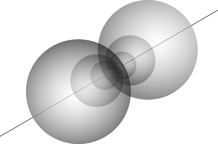
Example 1.1.
Let and let with for some nonzero . Consider the set of oriented spheres . Every pair of spheres from this set is in contact. See Figure 1.
Definition 1.2.
Let be a set of spheres, every pair of which is in contact. If is maximal (in the sense that no additional spheres can be added to while maintaining this property), then is called a “pencil of contacting spheres.” If is a set of oriented spheres and is a pencil of contacting spheres, we say that is -rich (with respect to ) if at least spheres from are contained in . We say is exactly -rich if exactly spheres from are contained in .
Remark 1.3.
If we identify each sphere in a pencil of contacting spheres with its coordinates , then the corresponding points form a line in . If we identify each sphere in a pencil of contacting spheres with its corresponding line in , then the resulting family of lines are all coplanar and pass through a common point (possibly at infinity111If two lines are parallel, then we say these lines pass through a common point at infinity.). This will be discussed further in Section 2.4.
The next result says that any two elements from a pencil of contacting spheres uniquely determine that pencil.
Lemma 1.4.
Let and be distinct oriented spheres that are in contact. Then the set of oriented spheres that are in contact with and is a pencil of contacting spheres.
We will defer the proof of Lemma 1.4 to Section 2.4. Example 1.1 suggests that rather than asking how many spheres from are in contact, we should instead ask how many -rich pencils can be determined by —each pencil that is exactly rich determines pairs of contacting spheres. We begin with the case . Since each pair of spheres can determine at most one pencil, a set of oriented spheres determines at most 2-rich pencils of contacting spheres. The next example shows that in general we cannot substantially improve this estimate, because there exist configurations of oriented spheres that determine -rich pencils.
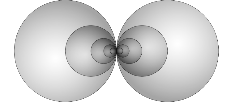
Example 1.5.
Let and be three spheres in , no two of which are in contact. Suppose that at least three spheres are in contact with each of and , and denote this set of spheres by . Let be the set of all spheres that are in contact with every sphere from . Then every sphere from is in contact with every sphere from and vice-versa. Furthermore, Lemma 1.4 implies that no two spheres from are in contact, and no two spheres from are in contact, so the spheres in do not determine any 3-rich pencils of contacting spheres. This means that if and , then determines 2-rich pencils of contacting spheres. See Figure 2.
Definition 1.6.
Let and be two sets of oriented spheres, each of cardinality at least three, with the property that each sphere from is in contact with each sphere from , and no two spheres from the same set are in contact. If and are maximal (in the sense that no additional spheres can be added to or while maintaining this property), then and are called a “pair of complimentary conic sections.”
Remark 1.7.
If we identify each sphere in a pair of complimentary conic sections with its coordinates , then the corresponding points are precisely the -points on a pair of conic sections in , neither of which are lines. If we identify each sphere in a pair of complimentary conic sections with its corresponding line in , then the resulting families of lines are contained in two rulings of a doubly-ruled surface in . Note, however, that the two rulings of this doubly-ruled surface contain additional lines that do not come from the pair of complimentary conic sections, since not all lines in the rulings will be contained in . This will be discussed further in Section 2.5.
We are now ready to state our main result. Informally, it asserts that the configurations described in Examples 1.1 and 1.5 are the only way that many pairs of spheres in can be in contact.
Theorem 1.8.
Let be a field in which is not a square. Let be a set of oriented spheres in , with (if has characteristic zero then we impose no constraints on ). Then for each , determines -rich pencils of contacting spheres. Furthermore, at least one of the following two things must occur:
-
•
There is a pair of complimentary conic sections so that
-
•
determines -rich pencils of contacting spheres.
Theorem 1.8 leads to new bounds for Erdős’ repeated distances problem in .
Theorem 1.9.
Let be a field in which is not a square. Let and let be a set of points in , with (if has characteristic zero then we impose no constraints on ). Then there are pairs satisfying
| (1.5) |
As discussed above, when the conjectured bound is and the current best known bound is [26]. For general fields in which is not a square, the previous best-known bound was .
Remark 1.10.
The bound given above cannot be improved without further restrictions on . Indeed, if we select to be a set of points in , then by pigeonholing there exists an element so that there are222Some care has to be taken when selecting the points in to ensure that not too many pairs of points satisfy , but this is easy to achieve. roughly solutions to (1.5). When is much smaller than (e.g. if ) it seems plausible that there should be solutions to (1.5).
Remark 1.11.
The requirement that not be a square is essential, since if is a square in then for each , the sphere is doubly-ruled by lines (see e.g. [21, Lemma 6]). It is thus possible to find an arrangement of spheres of radius , all of which contain a common line . Let , where is the set of centers of the spheres described above and is a set of points on . Then has pairs of points that satisfy (1.5).
Theorem 1.9 can also be used to prove new results for the incidence geometry of points and spheres in . In general, it is possible for points and spheres in to determine points-sphere incidences. For example, we can place points on a circle in and select spheres which contain that circle. The following definition, which is originally due to Elekes and Tóth [7] in the context of hyperplanes, will help us quantify the extent to which this type of situation occurs.
Definition 1.12.
Let be a field, let , and let be a real number. A sphere is said to be -non-degenerate (with respect to ) if for each plane we have .
Theorem 1.13 (Point-sphere incidences).
Let be a field in which is not a square. Let be a set of spheres (of nonzero radius) in and let be a set of points in , with (if has characteristic zero then we impose no constraints on ). Let and suppose the spheres in are -non-degenerate with respect to . Then there are incidences between the points in and the spheres in , where the implicit constant depends only on .
In [1], Apfelbaum and Sharir proved that points and -non-degenerate spheres in determine incidences, where the notation suppresses sub-polynomial factors. When , this bound simplifies to . Thus in the special case , Theorem 1.13 both strengthens the incidence bound of Apfelbaum and Sharir and extends the result from to fields in which is not a square. A construction analogous to the one from Remark 1.10 show that the bound cannot be improved unless we impose additional constraints on .
When , additional tools from incidence geometry become available, and we can say more.
Theorem 1.14.
Let a set of oriented spheres in . Then for each , determines -rich pencils of contacting spheres.
Note that a -rich pencil determines pairs of contacting spheres. Since the quantity is dyadically summable in , Theorem 1.14 allows us to bound the number of pairs of contacting spheres, provided not too many spheres are contained in a common pencil or pair of complimentary conic sections.
Corollary 1.15.
Let a set of oriented spheres in . Suppose that no pencil of contacting spheres is rich. Then at least one of the following two things must occur
-
•
There is a pair of complimentary conic sections so that
(1.6) -
•
There are pairs of contacting spheres.
The following (rather uninteresting) example shows that Theorem 1.14 can be sharp when there are pairs of complimentary conic sections that contain almost spheres from .
Example 1.16.
Let and let be a disjoint union , where for each index , each of and is a set of spheres contained in complimentary conic sections. The spheres in determine -rich pencils, and no pair of complimentary conic sections satisfy (1.6).
A similar example shows that Theorem 1.14 can be sharp when there are pencils that contain almost spheres from . More interestingly, the following “grid” construction shows that Theorem 1.14 can be sharp even when does not contain many spheres in a pencil or many spheres in complimentary conic sections.
Example 1.17.
Let , let , and let consist of all oriented spheres centered at of radius , where . We can verify that the equation
| (1.7) |
has roughly solutions. No linear pencil of contacting spheres contains more than spheres from . This means that determines roughly 2-rich pencils, and also determines roughly pairs of contacting spheres. On the other hand, if we fix three non-collinear points , , then the set of points satisfying (1.7) for each index must be contained in an irreducible degree two curve in . Bombieri and Pila [2] showed that such a curve contains points from . We conclude that every pair of complimentary conic sections contains spheres from .
1.1 Thanks
The author would like to thank Kevin Hughes and Jozsef Solymosi for helpful discussions, and Adam Sheffer for comments and corrections to an earlier version of this manuscript. The author would also like to thank Gilles Castel for assistance creating Figures 1 and 2. The author was partially funded by a NSERC discovery grant.
2 Lie’s line-sphere correspondence
In this section we will discuss the contact-incidence isomorphism introduced in Section 1. Throughout this section, will be a field in which is not a square, and is a degree-two extension of , where
2.1 Lines and the Klein quadric
In this section we will be concerned with points in and its projectivization . We will write elements of using the index set , and elements of will be denoted . Let be the symmetric bilinear form on given by
We define the Klein quadric to be the set
Since the polynomial is homogeneous, the above set is well-defined. Since , the above relation can also be written as
| (2.1) |
We will call this the Plücker relation.
There is a one-to-one correspondence between projective lines in and points in the Klein quadric. For our purposes, however, it will be more useful for us to identify a certain class of (affine) lines in with a large subset of the Klein quadric. Concretely, the (affine) line can be identified with the point
| (2.2) |
We will call this point the Plücker coordinates of the line. Conversely, the point with Plücker coordinates can be identified with the line .
Two lines and are coplanar (and thus either intersect or are parallel) if and only if their respective Plücker points and satisfy the relation .
2.2 Oriented spheres and the Lie quadric
In this section we will recall some basic facts from Lie sphere geometry. The primary reference is [3], especially Chapter 2, and [18]. Lie sphere geometry studies objects called “Lie spheres,” which unify the notion of a sphere, point, and plane (the latter two objects can be thought of as spheres that have zero and infinite radius, respectively). We will restrict attention to points and spheres.
Let be the symmetric bilinear form on defined by
We define the Lie quadric to be the set
Since the polynomial is homogeneous, the above set is well-defined. We will refer to the equation as as the Lie relation. It can also be written as
| (2.3) |
For each point with , we define the set
| (2.4) |
When , is the sphere defined by the equation
| (2.5) |
In particular, the oriented sphere centered at the point with radius can be identified with the point
| (2.6) |
A set of the form , with in the Lie Quadric will be referred to as a Lie sphere. We say that two Lie-spheres and are in “contact” if their corresponding Lie points and satisfy the relation , or equivalently
| (2.7) |
Indeed, examining (1.1), (2.6), and (2.7), we see that two oriented spheres and are in contact in the sense of (1.1) precisely when their corresponding Lie points satisfy .
2.3 Line-sphere correspondence
Consider the following map from the Lie quadric (which is a subset of ) to the Klein quadric (which is a subset of ). The point is mapped to
| (2.8) |
If , then
| (2.9) |
Setting , we see that if is an element of the Lie Quadric then is an element of the Klein Quadric. Furthermore, if and are distinct elements in the Lie Quadric, then the Lie spheres corresponding to and are in contact if and only if their images under are coplanar.
If is the oriented sphere centered at the point with radius , then by combining (2.6) and (2.8), we see that is mapped to the line in with Plücker coordinates
| (2.10) |
This corresponds to the line , where , , and . As we saw in Section 1, lines of this form are contained in the Heisenberg group .
2.4 Pencils of contacting spheres
In this section we will explore the structure of pencils of contacting spheres in , the Lie quadric, and the Heisenberg group. We will begin by proving Lemma 1.4. For the reader’s convenience we will restate it here.
Lemma 1.4.
Let and be distinct oriented spheres that are in contact. Then the set of oriented spheres that are in contact with and is a pencil of contacting spheres.
Proof.
We will prove the following equivalent statement: Let and be coplanar lines in the Heisenberg group that are not parallel to the plane. Let be the set of lines in the Heisenberg group not parallel to the plane that are coplanar with both and (so in particular . Then all of the lines in are contained in a common plane in and all pass through a common point (possibly at infinity). Furthermore, is maximal in the sense that no additional lines can be added to while maintaining the property that each pair of lines is coplanar.
First, observe that every line in that is not parallel to the plane points in a direction of the form , with . Every such line that points in the direction must be contained in the plane
| (2.11) |
In particular, this implies that any set of lines in that all point in the same direction and are not parallel to the plane must be contained in a common plane in .
Next, observe that if , then every line contained in passing through must be contained in the plane
| (2.12) |
If and are distinct points in , then the corresponding planes and are also distinct, and thus either are disjoint or intersect in a line. In particular, this implies that if two distinct lines contained in intersect at a point , then the unique plane in containing both lines is precisely .
Now, let and be three lines in that are pairwise coplanar. The following argument will show that and must be contained in a common plane and must pass through a common point (possibly at infinity).
First, if all three lines are parallel, then we have already shown that they are contained in a common plane and we are done. If not all three lines are parallel, then we can suppose that and intersect at a point , so and must be contained in . If is parallel to one of these lines, then without loss of generality we can suppose it is parallel to , and both lines point in direction . Then intersects two distinct lines contained in , so must also be contained in . But if , then this implies , which is impossible since . Thus we may suppose that is not parallel to either or . Suppose intersects and at distinct points. Then must also be contained in . But at least one of the points and must differ from , which implies there is a point with ; this is a contradiction. We conclude that passes through . Since all lines in passing through must be contained in , we conclude that and are coplanar and coincident.
It now immediately follows that if every line in is coplanar with both and , then each of these lines must either be parallel with and (if and are parallel), or must pass through their common intersection point (if and are not parallel). Furthermore, each line in must be contained in the plane spanned by and . In particular, all of the lines in are coplanar and pass through a common point (possibly at infinity). By construction the set is maximal, i.e. no additional lines can be added to while maintaining the property that all pairs of lines in are coplanar. ∎
If , then the set of lines in that are not parallel to the plane containing are of the form , where
| (2.13) |
The set of quadruples satisfying (2.13) belong to a line in ; we will call this line . Similarly, if , with , the set of lines in pointing in direction are of the form with . We will call this line .
Remark 2.1.
The above discussion implies that the spheres in a pencil of contacting spheres must either all have the same (signed) radius, or must all have different radii.
2.5 Complimentary conics
In this section we will discuss the structure of sets of spheres that form complimentary conics. The next lemma says that pencils of spheres and and pairs of complimentary conics are the only configurations allowing many spheres to be in contact.
Lemma 2.2.
Let and be sets of oriented spheres, each of cardinality at least three, so that every sphere in is in contact with every sphere in and vice-versa. Then either is contained in a pencil of contacting spheres (in which case every sphere in is in contact with every other sphere), or and are contained in complimentary conic sections.
Proof.
First, suppose that two spheres are in contact. Then by Proposition 1.4, the spheres in are contained in a pencil of contacting spheres. Since , we have that . Proposition 1.4 now implies that every sphere from is contained in . We conclude that is contained in a pencil of contacting spheres. An identical argument applies if two spheres are in contact. Thus we can suppose that no two spheres from are in contact, and no two spheres from are in contact. Let be the set of spheres in contact with each sphere from , and let be the set of spheres that are in contact with each sphere from ; we have that and are complimentary conics containing and , respectively. ∎
We will now consider the structure of a pair of complimentary conic sections. Let be elements of the Lie quadric, no two of which are in contact. Let and be the lines in corresponding to the images of and under . Let be the algebraic closure of (so in particular ), and let be the Zariski closure of in . Then and are skew lines in , and the set of lines in that are coplanar with each form a ruling of a doubly ruled surface in . Let be the set of lines in the ruling that contains the lines and and let be the set of lines in the other ruling. The sets and are irreducible conic curves in the variety . We then have and . Since is linear, this implies that and are precisely the -points of an irreducible curve in that is contained in the Lie quadric (or more precisely, contained in the variety ). Recalling the identification (2.5) of points in the Lie quadric with spheres in , we see that and correspond to sets of oriented spheres whose coordinates are contained in conic sections, neither of which are lines.
Note that for some triples it is possible that no elements of the Lie quadric will be in contact with each . This can happen, for example, if ; and correspond to disjoint spheres; and corresponds to a sphere contained inside . In this situation the complimentary conic sections and are well defined, but does not have any -points.
3 Incidence geometry in the Heisenberg group
In this section we will explore the incidence geometry of lines in the Heisenberg group. In particular, we will prove Theorems 1.8, 1.9, and 1.13. Our main tool is the following structure theorem for sets of lines in three space that determine many 2-rich points. The version stated here is Theorem 3.8 from [12]; a similar statement can also be found in [17].
Theorem 3.1.
There are absolute constants and so that the following holds. Let be a set of lines in , with (if has characteristic zero then we impose no constraints on ). Then for each , either determines at most -rich points, or there is a plane or doubly-ruled surface in that contains at least lines from .
Recall that lines contained in the Heisenberg group are somewhat special. In particular, Lemma 1.4 says that any set of pairwise coplanar lines must also pass through a common point (possibly at infinity). The next lemma is a version of Theorem 3.1 adapted to lines in the Heisenberg group. The hypotheses and conclusions of the theorem have also been slightly tweaked to better fit our needs for proving Theorems 1.8, 1.9, and 1.13.
Lemma 3.2.
There is an absolute constant so that the following holds. Let be a set of lines in the Heisenberg group that are not parallel to the plane, with (if has characteristic zero then we impose no constraints on ). Suppose that each line in is coloured either red or blue. Then for each , either there are at most points that are incident to at least one red and one blue line, or there is a doubly-ruled surface with one ruling that contains at least red lines and a second ruling that contains at least blue lines.
Proof.
Suppose that there are more than points that are incident to at least one red and one blue line (we will call such points bichromatic 2-rich points). We will show that if is chosen sufficiently large then there is a doubly-ruled surface with one ruling that contains at least red lines and a second ruling that contains at least blue lines.
Observe that Lemma 3.2 assumes that , while Theorem 3.1 places the more stringent requirement . Our first task will be to reduce the size of slightly. Without loss of generality we can assume that , since if then we can replace with and Theorem 3.1 remains true. Let be a set obtained by randomly keeping each element in with probability . With high probability, a set of this form will have cardinality at most and will will determine at least bichromatic 2-rich points, with . In particular, we can assume that has both of these properties.
Our next task is to prune the set slightly so that all of the unpruned lines contain many bichromatic 2-rich points. Define . For each index , let be obtained by removing a line from that contains at most bichromatic 2-rich points. If no such line exists, then halt. Observe that has cardinality and determines at least bichromatic 2-rich points. If is sufficiently large then this process must halt for some index with . Let be the resulting set; we have that determines at least bichromatic 2-rich points, with , and every line determines at least bichromatic 2-rich points.
Apply Theorem 3.1 to . If (and thus ) is chosen sufficiently large then there exists a plane or doubly-ruled surface that contains at least lines from ; Let be the set of lines from that are contained in . We claim that cannot be a plane; indeed if was a plane then by Lemma 1.4 the lines in must all intersect at a common point (possibly at infinity). In particular, each of the lines in contain at least 2-rich points, and at least of these 2-rich points must come from lines in . Thus the lines in must intersect in at least distinct points. Since each line in intersects in at most one point, this is impossible.
We conclude that is a doubly ruled surface. Since each line in that is not contained in can intersect in at most two points, by pigeonholing there exists a line that contains bichromatic 2-rich points, and at least of these points come from lines contained in the dual ruling of . Without loss of generality the line is red; this means that the ruling dual to contains at least blue lines. Again by pigeonholing, at least one of these blue lines contains bichromatic 2-rich points, and at least of these points come from lines contained in the ruling of dual to (i.e. the ruling that contains ). We conclude that the ruling containing must contain at least red lines. ∎
Corollary 3.3.
Let be a set of lines in the Heisenberg group that are not parallel to the plane, with (if has characteristic zero then we impose no constraints on ). Then either determines 2-rich points, or there is a doubly-ruled surface, each of whose rulings contain at least lines from .
Proof.
Suppose that determines 2-rich points. Randomly colour each line in either red or blue. With high probability determines at least bichromatic 2-rich points. If is sufficiently large, then Lemma 3.3 implies that there is a doubly-ruled surface, each of whose rulings contain at least lines from . ∎
Lemma 3.2 allows us to understand configurations of lines in that contain many bichromatic 2-rich points. The next lemma concerns configurations of lines in that contain many -rich points for . Since the proof of the next lemma is very similar to that of Lemma 3.2 (in particular it uses the same ideas of random sampling and refinement), we will just provide a brief sketch that highlights where the proofs differ.
Lemma 3.4.
Let be a set of lines in the Heisenberg group that are not parallel to the plane, with (if has characteristic zero then we impose no constraints on ). Let . Then determines -rich points.
Proof sketch.
Let be obtained by randomly selecting each line with probability . Then with positive probability we have that , and the number of 3-rich points determined by is at least half the number of -rich points determined by . We now argue as in the proof of Corollary 3.3; if determines 3-rich points, then there must exist a doubly-ruled surface that contains lines from , and each of these lines must contain at least 3-rich points. In particular, there must be at least 3-rich points contained in . Since is doubly (not triply!) ruled, this means that each of these 3-rich points must be incident to a line from that is not contained in . Since each line in not contained in can intersect in at most 2 points, the number of 3-rich points created in this way is at most , which is a contradiction. ∎
With these preliminary results established, we are now ready to prove the main results of this section.
Proof of Theorem 1.8.
First, using the line-sphere correspondence described in Section 2.3, Theorem 1.8 is implied by the following statement about lines in the Heisenberg group:
Let be a set of lines in the Heisenberg group that are not parallel to the plane, with (if has characteristic zero then we impose no constraints on ). Then for each , there are -rich points. Furthermore, at least one of the following two things must occur:
-
•
There is a doubly-ruled surface, each of whose ruling contain at least lines from .
-
•
determines -rich points.
The theorem now follows immediately from Corollary 3.3 and Lemma 3.4. ∎
Our proof of Theorem 1.9 will follow a similar strategy to the proof of Theorem 1.8. The main thing to verify is that not too many lines can be contained in a doubly-ruled surface.
Proof of Theorem 1.9.
Let be three points. Consider the set of points satisfying
| (3.1) | ||||
| (3.2) | ||||
| (3.3) |
Note that these three equations are satisfied precisely when
where
| (3.4) |
In particular, since is not a square in , the set does not contain any lines (see e.g. [21, Lemma 6]), so (3.1), (3.2), and (3.3) have no solutions when the points are collinear.
Note that the vectors and are parallel precisely if the points , , and are collinear (and thus there are no solutions to (3.1),(3.2), and (3.3)).
If and are not parallel, then the set of points satisfying (3.1), (3.2), and (3.3) is precisely the set of points satisfying (3.1), (3.5), and (3.6); this is the intersection of a line and a sphere of radius . Again, since a sphere of radius cannot contain any lines, this intersection consists of at most 2 points. To summarize,
| (3.7) |
Let , where is the map defined in Section 2.3, and we identify a point with the corresponding sphere of zero radius. Let , where is the sphere with center and radius .
Apply Lemma 3.2 to , where the first set of lines is coloured red and the second set is coloured blue. The bound (3.7) shows that there cannot exist a doubly-ruled surface with three red lines in one ruling and three blue lines in the other ruling. We conclude that determines bichromatic 2-rich points. Thus there are pairs of points from that satisfy (1.5). ∎
Finally, we will prove Theorem 1.13. The main observation is that while a pencil that is exactly -rich determines pairs of tangent spheres, this pencil only determines or fewer point-sphere incidences (i.e. at most tangencies between a sphere of zero radius and a sphere of nonzero radius).
Proof of Theorem 1.13.
Let be the set of lines associated to the points from (i.e. spheres of radius 0), and let be the set of lines associated to the spheres from . Observe that by Remark 2.1, each -rich pencil can contribute at most point-sphere incidences. Applying Lemma 3.4 to , we see that for each the set of pencils of richness between and can contribute at most incidences. Summing dyadically in , we conclude that the set of pencils of richness at least 3 can contribute incidences.
It remains to control the number of incidences arising from 2-rich points. Let . With this choice of , apply Lemma 3.2 to , where the first set of lines is coloured red and the second set is coloured blue. If contains bichromatic 2-rich points then we are done. If not, then there is a doubly-ruled surface with one ruling that contains at least red lines and a second ruling that contains at least blue lines. Let be the set of blue lines from one of these rulings (recall that blue lines correspond to spheres from . Recall that each red line in that is not contained in intersects in at most two points. Thus since , by pigeonholing there must exist a line that is incident to fewer than lines from that are not contained in . This implies that the corresponding sphere is not -non-degenerate, which contradicts the assumption that all of the spheres in are -non-degenerate. ∎
4 Improvements over
In this section we will show how Theorem 1.8 can be improved when . The main tool will be the following polynomial partitioning theorem due to Guth [9].
Theorem 4.1.
Let be a set of real algebraic varieties in , each of which has dimension and is defined by a polynomial of degree at most . Then for each , there is a -variate “partitioning” polynomial of degree at most so that is a disjoint union of “cells” (open connected sets), and each of these cells intersect varieties from . The implicit constant depends on and , but (crucially) is independent of and .
While the definition of the dimension of a real algebraic variety is slightly technical, we will only use the elementary facts that points in are algebraic varieties of dimension 0 and lines are algebraic varieties of dimension 1. Applying Theorem 4.1 to a set of points and to a set of lines in (with parameter in each case) and taking the product of the resulting partitioning polynomials, we obtain a polynomial whose zero-set efficiently partitions a set of points and a set of lines simultaneously. We will record this observation below.
Corollary 4.2.
Let be a set of points in and let be a set of lines in . Then for each , there is a polynomial of degree at most so that is a disjoint union of cells; each cell contains points from ; and each cell intersects lines from .
Note that while Corollary 4.2 guarantees that few points are contained in each cell and few lines meet each cell, it is possible that many points and lines are contained in the “boundary” of the cells. The next lemma helps us understand what configurations of points and lines are possible inside .
Lemma 4.3.
Let be irreducible and let . If is not a plane, then there are at most “bad” lines contained in . If is not a bad line, then there are “bad” points . If is not a bad point, then it is incident to at most one additional line that is contained in .
Proof.
Statements of this form appear frequently in the literature (see e.g. Theorem 1.9 from [23]), and follow directly from the machinery of Guth and the author developed in [12]. We will briefly outline the proof here. We say a point is 3-flecnodal if there are at least three distinct lines that contain and are contained in . If a line contains more than 3-flecnodal lines for some absolute constant , then all but finitely many points of must be 3-flecnodal (i.e. a Zariski-dense subset of is 3-flecnodal). If there are lines , each of which is 3-flecnodal at all but finitely many points, then there is a Zariski-dense subset so that for each point there are at least three lines containing and contained in . But since is irreducible, this immediately implies that is a plane. ∎
The next two lemmas will help us understand the incidence geometry of configurations of coplanar lines coming from the Heisenberg group. Recall that throughout this section, and .
Lemma 4.4.
Let be a set of points with . Suppose that every pair of points is connected by a line in the Heisenberg group. Then is contained in a (complex) line.
Proof.
Let . Define and define similarly. Then (resp. ) is precisely the intersection of with the tangent plane of at (resp. ). In particular, is contained in a complex line, and . Since the choice of and was arbitrary, we conclude that every subset of cardinality is collinear. Since this implies that all the points of are collinear. ∎
Lemma 4.5.
Let be a set of points and let be a set of lines in the Heisenberg group that are not parallel to the plane. Then
| (4.1) |
Proof.
By Corollary 3.4, for each the number of -rich points determined by is . Since a -rich point contributes incidences, we conclude that the number of incidences coming from points with richness is . The number of incidences coming from points with richness is at most . ∎
We are now ready to prove the main result of this section.
Proposition 4.6.
Let be a set of points and let be a set of lines in the Heisenberg group that are not parallel to the plane. Then
| (4.2) |
where is an absolute constant
Proof.
Our proof is closely modeled on the techniques of Sharir and Zlydenko from [23]. We will prove the result by induction on ; the base case for our induction will be when , where is an absolute constant to be specified below. Observe that if for a fixed constant , then then the result follows from Lemma 4.5; indeed, if then and thus
Henceforth we will assume that
| (4.3) |
where is a constant that will be specified below.
For each line of the form , let be the point . Define
For each point , let be the line described by (2.13). Define
By Lemma 4.5, for any set of points and any set of lines , we have the incidence bound
| (4.4) |
Let be a surjective linear map; we will choose this map so that the image of every line in remains a line, and no additional incidences are added. We will abuse notation slightly by replacing with the set (so now ) and replacing with the set (so now is a set of lines in ). Note that (4.4) remains true with these new definitions of and .
Define
| (4.5) |
where is the same constant as in (4.3). In the analysis that follows, “Case 1” will refer to the situation where , and “Case 2” will refer to the situation where .
Observe that Indeed, in Case 1 we have and thus . In Case 2 we have , and again . If we select , then we have ensured that . Inequality (4.3) implies that ; thus we can assume that . In summary, we have
| (4.6) |
Apply Corollary 4.2 to and with this choice of ; we obtain a partitioning polynomial . is a union of cells, each of which contains points from and each of which intersects line from .
In Case 1, we use (4.4) to control the number of point-line incidences inside the cells. If we index the cells with and define to be the set of lines from that intersect , then
| (4.7) |
In Case 2 each cell meets lines, and thus
| (4.8) |
Let , where consists of the lines not contained in and consists of the lines contained in . Since each line in can intersect at most times, we have
| (4.9) |
Our next task is to control the number of incidences formed by lines in . Factor into irreducible components , where the polynomials each have degree at least two and the polynomials have degree one (it is possible that all polynomials have degree at least two or no polynomials have degree at least two. In the former case we set and in the latter case we set ). For each index , define
We have . Similarly, let be the set of lines that are contained in and are not contained in for any index .
If for some and with , then the line must intersect , and cannot be contained in . Since can intersect in at most points, we can bound the number of such “cross-index” incidences as follows.
| (4.10) |
It remains to control incidences where and . Let consist of those points that are incident to at least 3 lines from . Define . By Lemma 4.3, for each index there are “bad” lines for some absolute constant . For each index , let be the set of bad lines associated to and let . If we choose the constant from (4.5) sufficiently small, then
Thus by the induction hypothesis we have
If then can be incident to at most bad points, for some absolute constant . Since
we have
If then can be incident to at most two lines from . Thus as long as we have
| (4.11) |
Proof of Theorem 1.14.
Let and let . We need to prove that determines -rich points. When is small the result follows from Theorem 1.8, so we can assume that , for some absolute constant to be determined later. Let be the set of -rich points determined by , and let . We clearly have . On the other hand, Proposition 4.6 implies that
| (4.14) |
Thus if the constant is selected sufficiently large compared to the implicit constant in (4.14), then , as desired. ∎
References
- [1] R. Apfelbaum and M. Sharir. Non-degenerate spheres in three dimensions. Combin. Prob. Comput., 20:503–512, 2011.
- [2] E. Bombieri and J. Pila. The number of integral points on arcs and ovals. Duke Math. J., 59:337–357, 1989.
- [3] T. E. Cecil. Lie Sphere Geometry. Springer, 1992.
- [4] K. Clarkson, H. Edelsbrunner, L. Guibas, M. Sharir, and E. Welzl. Combinatorial complexity bounds for arrangements of curves and surfaces. Discrete Comput. Geom, 5:99–160, 1990.
- [5] F. de Zeeuw. A short proof of Rudnev’s point-plane incidence bound. arXiv:1612.02719, 2016.
- [6] Z. Dvir. On the size of Kakeya sets in finite fields. J. Amer. Math. Soc., 22:1093–1097, 2009.
- [7] G. Elekes and C. D. Tóth. Incidences of not too degenerate hyperplanes. In Proc. 21st Annu. ACM Sympos. Comput. Geom., pages 16–21, 2005.
- [8] P. Erdős. On sets of distances of points in Euclidean space. Magyar Tudományos Akadémia Matematikai Kutató Intézet Közleményei, 5:165–169, 1960.
- [9] L. Guth. Polynomial partitioning for a set of varieties. Math. Proc. Camb. Philos. Soc., 159:459–469, 2015.
- [10] L. Guth. Polynomial Methods in Combinatorics. AMS, 2018.
- [11] L. Guth and N. Katz. Algebraic methods in discrete analogs of the Kakeya problem. Adv. Math., 225:2828–2839, 2010.
- [12] L. Guth and J. Zahl. Algebraic curves, rich points, and doubly-ruled surfaces. Amer. J. Math., 140:1187–1229, 2018.
- [13] H. Kaplan, J. Matoušek, Z. Safernová, and M. Sharir. Unit distances in three dimensions. Combin. Prob. Comput., 21:597–610, 2012.
- [14] H. Kaplan, M. Sharir, and E. Shustin. On lines and joints. Discrete. Comput. Geom., 44:838–843, 2010.
- [15] N. Katz, I. Łaba, and T. Tao. An improved bound on the Minkowski dimension of Besicovitch sets in . Ann. of Math., 152:383–446, 2000.
- [16] N. Katz and J. Zahl. An improved bound on the Hausdorff dimension of Besicovitch sets in . J. Amer. Math. Soc., 32:195–259, 2019.
- [17] J. Kollár. Szemerédi–Trotter-type theorems in dimension 3. Adv. Math., 271:30–61, 2015.
- [18] R. Milson. An overview of Lie’s line-sphere correspondence. In J. Leslie and T. Robart, editors, The geometrical study of differential equations, pages 129–162. AMS, 2001.
- [19] G. Mockenhaupt and T. Tao. Restriction and Kakeya phenomena for finite fields. Duke Math. J., 121:35–74, 2004.
- [20] M. Rudnev. On the number of incidences between points and planes in three dimensions. Combinatorica, 38:219–254, 2018.
- [21] M. Rudnev. Point-plane incidences and some applications in positive characteristic. In K. Schmidt and A. Winterhof, editors, Combinatorics and Finite Fields: Difference Sets, Polynomials, Pseudorandomness and Applications, pages 211–240. De Gruyter, 2019.
- [22] M. Rudnev and J. Selig. On the use of Klein quadric for geometric incidence problems in two dimensions. SIAM J. Discrete Math., 30:934–954, 2014.
- [23] M. Sharir and O. Zlydenko. Incidences between points and curves with almost two degrees of freedom. In Proc. 36th Annu. ACM Sympos. Comput. Geom., 2020.
- [24] T. Tao. Stickiness, graininess, planiness, and a sum-product approach to the kakeya problem. https://terrytao.wordpress.com/2014/05/07/stickiness-graininess-planiness-and-a-sum-product-approachto-the-kakeya-problem, 2014.
- [25] J. Zahl. An improved bound on the number of point-surface incidences in three dimensions. Contrib. Discrete Math., 8:100–121, 2013.
- [26] J. Zahl. Breaking the 3/2 barrier for unit distances in three dimensions. Int. Math. Res. Not., Vol 2019:6235–6284, 2019.