New Discontinuous Galerkin Algorithms and Analysis for Linear Elasticity with Symmetric Stress Tensor

Abstract

This paper presents a new and unified approach to the derivation and analysis of many existing, as well as new discontinuous Galerkin methods for linear elasticity problems. The analysis is based on a unified discrete formulation for the linear elasticity problem consisting of four discretization variables: strong symmetric stress tensor $\bm{\sigma}_{h}$ and displacement $u_{h}$ inside each element, and the modifications of these two variables $\check{\bm{\sigma}}_{h}$ and $\check{u}_{h}$ on elementary boundaries of elements. Motivated by many relevant methods in the literature, this formulation can be used to derive most existing discontinuous, nonconforming and conforming Galerkin methods for linear elasticity problems and especially to develop a number of new discontinuous Galerkin methods. Many special cases of this four-field formulation are proved to be hybridizable and can be reduced to some known hybridizable discontinuous Galerkin, weak Galerkin and local discontinuous Galerkin methods by eliminating one or two of the four fields. As certain stabilization parameter tends to zero, this four-field formulation is proved to converge to some conforming and nonconforming mixed methods for linear elasticity problems. Two families of inf-sup conditions, one known as $H^{1}$-based and the other known as $H({\rm div})$-based, are proved to be uniformly valid with respect to different choices of discrete spaces and parameters. These inf-sup conditions guarantee the well-posedness of the new proposed methods and also offer a new and unified analysis for many existing methods in the literature as a by-product. Some numerical examples are provided to verify the theoretical analysis including the optimal convergence of the new proposed methods.

1 Introduction

In this paper, we introduce a unified formulation and analysis for linear elasticity problems

$$\left\{\begin{aligned} A\bm{\sigma}-\epsilon(u)&=0\quad&\text{ in }{\rm\Omega},\\ {\rm div}\bm{\sigma}&=f\quad&\text{ in }{\rm\Omega},\\ u&=0\quad&\text{ on }\Gamma_{D},\\ \bm{\sigma}n&=0\quad&\text{ on }\Gamma_{N},\end{aligned}\right.$$ (1)

with ${\rm\Omega}\subset\mathbb{R}^{n}~{}(n=2,3)$ and $\partial{\rm\Omega}=\Gamma_{D}\cup\Gamma_{N}$, $\Gamma_{D}\cap\Gamma_{N}=\varnothing$. Here the displacement is denoted by $u:{\rm\Omega}\rightarrow\mathbb{R}^{n}$ and the stress tensor is denoted by $\bm{\sigma}:{\rm\Omega}\rightarrow\mathcal{S}$, where $\mathcal{S}$ is the set of symmetric $n\times n$ tensors. The linearized strain tensor $\epsilon(u)=\frac{1}{2}(\nabla u+\nabla u^{T})$. The compliance tensor $A:\mathcal{S}\rightarrow\mathcal{S}$

$$A\bm{\sigma}={1+\nu\over E}\bm{\sigma}-{(1+\nu)\nu\over(1+(n-2)\nu)E}tr(\bm{\sigma})I$$ (2)

is assumed to be bounded and symmetric positive definite, where $E$ and $\nu\in(0,\frac{1}{2})$ are the Young’s modulus and the Poisson’s ratio of the elastic material under consideration, respectively.

Finite element method (FEM) and its variants have been widely used for numerical solutions of partial differential equations. Conforming and nonconforming FEMs in primal form are two classic Galerkin methods for elasticity and structural problems hrennikoff1941solution ; courant1994variational ; feng1965finite . Mixed FEMs for the elasticity problem, derived from the Hellinger-Reissner variational principle, are also popular methods since they approximate not only the displacement but also the stress tensor. Unlike the mixed FEMs for scalar second-order elliptic problems, the strong symmetry is required for the stress tensor in the elasticity problem. This strong symmetry causes a substantial additional difficulty for developing stable mixed FEMs for the elasticity problem. To overcome such a difficulty, it was proposed in Fraejis1975 to relax or abandon the symmetric constraint on the stress tensor by employing Lagrangian functionals. This idea was developed in late nineteens amara1979equilibrium ; arnold1984peers ; arnold1988new ; stein1990mechanical ; stenberg1986construction ; stenberg1988family ; stenberg1988two , and further systematically explored in a recent work arnold2007mixed by utilizing a constructive derivation of the elasticity complex starting from the de Rham complex eastwood2000complex and mimicking the construction in the discrete case. Another framework to construct stable weakly symmetric mixed finite elements was presented in boffi2009reduced , where two approaches were particularly proposed with the first one based on the Stokes problem and the second one based on interpolation operators. To keep the symmetry of discrete stress, a second way is to relax the continuity of the normal components of discrete stress across the internal edges or faces of grids. This approach leads to nonconforming mixed FEMs with strong symmetric stress tensor yi2005nonconforming ; yi2006new ; man2009lower ; hu2007lower ; awanou2009rotated ; arnold2003nonconforming ; arnold2014nonconforming ; gopalakrishnan2011symmetric ; wu2017interior ; hu2019nonconforming . In 2002, based on the elasticity complex, the first family of symmetric conforming mixed elements with polynomial shape functions was proposed for the two-dimensional case in arnold2002mixed , which was extended to the three-dimensional case in arnold2008finite . Recently, a family of conforming mixed elements with fewer degrees of freedom was proposed for any dimension by discovering a crucial structure of discrete stress spaces of symmetric matrix-valued polynomials on any dimensional simplicial grids and proving two basic algebraic results in hu2014family ; hu2015family ; hu2016finite ; hu2014finite . Those new elements can be regarded as an improvement and a unified extension to any dimension of those from arnold2002mixed and arnold2008finite , without an explicit use of the elasticity complex. Besides the optimal convergence property with respect to the degrees of polynomials of discrete stresses, an advantage of those elements is that it is easy to construct their basis functions, therefore implement the elements. See stabilized mixed finite elements on simplicial grids for any dimension in chen2017stabilized .

Discontinuous Galerkin (DG) methods were also widely used in numerical solutions for the elasticity problem, see chen2010local ; hong2016robust ; hong2019conservative ; wang2020mixed . DG methods offer the convenience to discretize problems in an element-by-element fashion and use numerical traces to glue each element together arnold2002unified ; hong2012discontinuous ; hong2016uniformly ; hong2018parameter . This advantage makes DG methods an ideal option for linear elasticity problems to preserve the strong symmetry of the stress tensor. Various hybridizable discontinuous Galerkin (HDG) formulations with strong symmetric stress tensor were proposed and analyzed for linear elasticity problems, such as soon2008hybridizable ; soon2009hybridizable ; fu2015analysis ; qiu2018hdg ; chen2016robust . The HDG methods for linear elasticity problems contain three variables – stress $\bm{\sigma}_{h}$, displacement $u_{h}$ and numerical trace of displacement $\hat{u}_{h}$. In the HDG methods, the variable $\hat{u}_{h}$ is defined on element borders and can be viewed as the Lagrange multiplier for the continuity of the normal component of stress. Weak Galerkin (WG) methods were proposed and analyzed in wang2016locking ; wang2018weak ; wang2018hybridized ; chen2016robust ; yi2019lowest for linear elasticity problems. The main feature of the WG methods is the weakly defined differential operators over weak functions. A three-field decomposition method was discussed for linear elasticity problems in brezzi2005three . A new hybridized mixed method for linear elasticity problems was proposed in gong2019new .

Virtual element method is a new Galerkin scheme for the approximation of partial differential equation problems, and admits the flexibility to deal with general polygonal and polyhedral meshes. Virtual element method is experiencing a growing interest towards structural mechanics problems, and has contributed a lot to linear elasticity problems, see da2013virtual ; artioli2017stress ; artioli2018family ; dassi2020three and the reference therein. Recently, investigation of the possible interest in using virtual element method for traditional decompositions is presented in brezzi2021finite . As shown in brezzi2021finite , virtual element method looks promising for high-order partial differential equations as well as Stokes and linear elasticity problems. Some other interesting methods, say the tangential-displacement normal-normal-stress method which is robust with respect both shear and volume locking, were considered in pechstein2011tangential ; pechstein2018analysis .

In this paper, a unified formulation is built up for linear elasticity problems following and modifying the ones in hong2020extended ; hong2021extended for scalar second-order elliptic problems. The formulation is given in terms of four discretization variables — $\bm{\sigma}_{h}$, $\check{\bm{\sigma}}_{h}$, $u_{h}$, $\check{u}_{h}$. The variables $\bm{\sigma}_{h}$ and $u_{h}$ approximate the stress tensor $\bm{\sigma}$ and displacement $u$ in each element, respectively. Strong symmetry of the stress tensor is guaranteed by the symmetric shape function space of the variable $\bm{\sigma}_{h}$. The variables $\check{\bm{\sigma}}_{h}$ and $\check{u}_{h}$ are the residual corrections to the average of $\bm{\sigma}_{h}$ and $u_{h}$ along interfaces of elements, respectively. They can also be viewed as multipliers to impose the inter-element continuity property of $u_{h}$ and the normal component of $\bm{\sigma}_{h}$, respectively. The four variables in the formulation provide feasible choices of numerical traces, and therefore, the flexibility of recovering most existing FEMs for linear elasticity problems. There exist two different three-field formulations by eliminating the variable $\check{\bm{\sigma}}_{h}$ and $\check{u}_{h}$, respectively, and a two-field formulation by eliminating both. With the same choice of discrete spaces and parameters, these four-field, three-field, and two-field formulations are equivalent. Moreover, some particular discretizations induced from the unified formulation are hybridizable and lead to the corresponding one-field formulation.

As shown in hong2019unified ; hong2018uniform ; hong2020extended , the analysis of the formulation is classified into two classes: $H^{1}$-based class and $H({\rm div})$-based class. Polynomials of a higher degree for the displacement than those for the stress tensor are employed for the $H^{1}$-based formulation and the other way around for the $H({\rm div})$-based formulation. Both classes are proved to be well-posed under natural assumptions. Unlike scalar second order elliptic problems, there is no stable symmetric $H({\rm div})$-conforming mixed finite elements in the literature that approximates the stress tensor by polynomials with degree not larger than $k$ and $k\leq n$. This causes the difficulty to prove the inf-sup condition for the $H({\rm div})$-based formulation with $k\leq n$. The nonconforming element in wu2017interior is employed here to circumvent this difficulty with the jump of the normal component of $\bm{\sigma}_{h}$ embedded in the norm of the stress tensor $\bm{\sigma}_{h}$.

The unified formulation is closely related to some mixed element methods. As some parameters approach zero, some mixed element methods and primal methods can be proven to be the limiting cases of the unified formulation. In particular, both the nonconforming mixed element method in gopalakrishnan2011symmetric and the conforming mixed element methods in hu2014finite ; hu2014family ; hu2015family are some limiting cases of the formulation. The proposed four-field formulation is also closely related to most existing methods qiu2018hdg ; chen2016robust ; soon2009hybridizable ; fu2015analysis ; chen2010local ; wang2020mixed for linear elasticity as listed in the first three rows in Table 2, and the first row in Table 3 and Table 4. More importantly, some new discretizations are derived from this formulation as listed in Table 1. Under the unified analysis of the four-field formulation, all these new methods are well-posed and admit optimal error estimates. In Table 1, the first scheme is an $H^{1}$-based method and the following two schemes are $H({\rm div})$-based methods. The last scheme is a special case of the second one with $\gamma=0$ and $\eta=\tau^{-1}$. The last scheme is hybridizable and can be written as a one-field formulation with only one globally-coupled variable. In fact, after the elimination of variable $\check{\sigma}_{h}$ and a transformation from variable $\check{u}_{h}$ to variable $\hat{u}_{h}$ in the last method of Table 1, we obtain an optimal $H({\rm div})$-based HDG method.

The notation $\tau=\Omega(h_{e}^{-1})$ and $\tau=\Omega(h_{e})$ in Table 1 means there exist constants $c_{0}>0,C_{0}>0$ such that $c_{0}h_{e}^{-1}\leq\tau\leq C_{0}h_{e}^{-1}$ and $c_{0}h_{e}\leq\tau\leq C_{0}h_{e}$, respectively. For $k\geq 0$,

$$V^{k}_{h} =\{v_{h}\in L^{2}(\Omega,\mathbb{R}^{n}):v_{h}|_{K}\in\mathcal{P}_{k}(K,\mathbb{R}^{n}),\forall K\in\mathcal{T}_{h}\},$$ (3)

$$Q^{k}_{h} =\{\bm{\tau}_{h}\in L^{2}(\Omega,\mathcal{S}):\bm{\tau}_{h}|_{K}\in\mathcal{P}_{k}(K,\mathcal{S}),\forall K\in\mathcal{T}_{h}\},$$

$$\check{V}^{k}_{h} =\{\check{v}_{h}\in L^{2}({\mathcal{E}_{h}},\mathbb{R}^{n}):v_{h}|_{e}\in\mathcal{P}_{k}(e,\mathbb{R}^{n}),\forall e\in{\mathcal{E}_{h}},\ \check{v}_{h}|_{\Gamma_{D}}=0\},$$

$$\check{Q}^{k}_{h} {=\{\check{\bm{\tau}}_{h}\in L^{2}({\mathcal{E}_{h}},\mathcal{S}):\check{\bm{\tau}}_{h}|_{e}\in\bm{\mathcal{P}}_{k}(e,\mathcal{S}),\forall e\in{\mathcal{E}_{h}},\ \check{\bm{\sigma}}_{h}n|_{\Gamma_{N}}=0\},}$$

where $\bm{\mathcal{P}}_{k}(K,\mathbb{R}^{n})$ and $\bm{\mathcal{P}}_{k}(e,\mathbb{R}^{n})$ are vector-valued in $\mathbb{R}^{n}$ and each component is in the space of polynomials of degree at most $k$ on $K$ and $e$, respectively, and $\bm{\mathcal{P}}_{k}(K,\mathcal{S})$ are symmetric tensor-valued functions in $\mathcal{S}$ and each component is in the space of polynomials of degree at most $k$ on $K$.

	$\eta$	$\tau$	$\gamma$	$Q_{h}$	$V_{h}$	$\check{Q}_{h}$	$\check{V}_{h}$
1	$\mathcal{O}(h_{e})$	$\mathcal{O}(h_{e}^{-1})$	$\mathcal{O}(1)$	$Q_{h}^{k}$	$V_{h}^{k+1}$	$\check{Q}_{h}^{r}$	$\check{V}_{h}^{k}$
2	$\mathcal{O}(h_{e}^{-1})$	$\mathcal{O}(h_{e})$	$\mathcal{O}(1)$	$Q_{h}^{k+1}$	$V_{h}^{k}$	$\{0\}\ \text{or}\ \check{Q}_{h}^{m}$	$\check{V}_{h}^{k+1}$
3	$\tau^{-1}$	$\Omega(h_{e})$	0	$Q_{h}^{k+1}$	$V_{h}^{k}$	$\check{Q}_{h}^{k}$	$\check{V}_{h}^{k+1}$

Table 1: New proposed methods with $r\geq\max(1,k)$ and $m\geq 0$. For the second and third schemes, $\|\bm{\sigma}-\bm{\sigma}_{h}\|_{\rm div,h}=\mathcal{O}(h^{k+1})$ for any $k\geq 0$ and $\|\bm{\sigma}-\bm{\sigma}_{h}\|_{0}=\mathcal{O}(h^{k+2})$ if $k\geq n$.

Throughout this paper, we shall use letter $C$, which is independent of mesh-size $h$ and stabilization parameters $\eta,\tau,\gamma$, to denote a generic positive constant which may stand for different values at different occurrences. The notation $x\lesssim y$ and $x\gtrsim y$ means $x\leq Cy$ and $x\geq Cy$, respectively. Denote $x\lesssim y\lesssim x$ by $x\eqsim y$.

The rest of the paper is organized as follows. Some notation is introduced in Section 2. In Section 3, a four-field unified formulation is derived for linear elasticity problems. By proving uniform inf-sup conditions under two sets of assumptions, an optimal error analysis is provided for this unified formulation. Section 4 derives some variants of this four-field formulation, and reveals their relation with some existing methods in the literature. Section 5 illustrates two limiting cases of the unified formulation: mixed methods and primal methods. Numerical results are provided in Section 6 to verify the theoretical analysis including the optimal convergence of the new proposed methods. Some conclusion remarks are given in Section 7.

2 Preliminaries

Given a nonnegative integer $m$ and a bounded domain $D\subset\mathbb{R}^{n}$, let $H^{m}(D)$, $\|\cdot\|_{m,D}$ and $|\cdot|_{m,D}$ be the usual Sobolev space, norm and semi-norm, respectively. The $L^{2}$-inner product on $D$ and $\partial D$ are denoted by $(\cdot,\cdot)_{D}$ and $\langle\cdot,\cdot\rangle_{\partial D}$, respectively. Let $\|\cdot\|_{0,D}$ and $\|\cdot\|_{0,\partial D}$ be the norms of Lebesgue spaces $L^{2}(D)$ and $L^{2}(\partial D)$, respectively. The norms $\|\cdot\|_{m,D}$ and $|\cdot|_{m,D}$ are abbreviated as $\|\cdot\|_{m}$ and $|\cdot|_{m}$, respectively, when $D$ is chosen as $\Omega$.

Suppose that ${\rm\Omega}\subset\mathbb{R}^{n}$ is a bounded polygonal domain covered exactly by a shape-regular partition ${\mathcal{T}_{h}}$ of polyhedra. Let $h_{K}$ be the diameter of element $K\in{\mathcal{T}_{h}}$ and $h=\max_{K\in{\mathcal{T}_{h}}}h_{K}$. Denote the set of all interior edges/faces of ${\mathcal{T}_{h}}$ by ${\mathcal{E}_{h}^{I}}$, and all edges/faces on boundary $\Gamma_{D}$ and $\Gamma_{N}$ by ${\mathcal{E}_{h}^{D}}$ and ${\mathcal{E}_{h}^{N}}$, respectively. Let ${\mathcal{E}_{h}}={\mathcal{E}_{h}^{I}}\cup{\mathcal{E}_{h}^{D}}\cup{\mathcal{E}_{h}^{N}}$ and $h_{e}$ be the diameter of edge/face $e\in{\mathcal{E}_{h}}$. For any interior edge/face $e=K^{+}\cap K^{-}$, let $n^{i}$ = $n|_{\partial K^{i}}$ be the unit outward normal vector on $\partial K^{i}$ with $i=+,-$. For any vector-valued function $v_{h}$ and matrix-valued function $\bm{\tau}_{h}$, let $v_{h}^{\pm}$ = $v_{h}|_{\partial K^{\pm}}$, $\bm{\tau}_{h}^{\pm}$ = $\bm{\tau}_{h}|_{\partial K^{\pm}}$. Define the average $\{\cdot\}$ and the jump $[\cdot]$ on interior edges/faces $e\in{\mathcal{E}_{h}^{I}}$ as follows:

$$\begin{array}[]{ll}\{\bm{\tau}_{h}\}=\frac{1}{2}(\bm{\tau}_{h}^{+}+\bm{\tau}_{h}^{-}),&[\bm{\tau}_{h}]=\bm{\tau}_{h}^{+}n^{+}+\bm{\tau}_{h}^{-}n^{-},\\ \{v_{h}\}=\frac{1}{2}(v_{h}^{+}+v_{h}^{-}),&[v_{h}]=v_{h}^{+}\odot n^{+}+v_{h}^{-}\odot n^{-}-(v_{h}^{+}\cdot n^{+}+v_{h}^{-}\cdot n^{-})\bm{I}\end{array}$$ (4)

where $v_{h}\odot n=v_{h}n^{T}+nv_{h}^{T}$ and $\bm{I}$ is the identity tensor. For any boundary edge/face $e\subset\partial\Omega$, define

$$\begin{array}[]{lllll}\{\bm{\tau}_{h}\}=\bm{\tau}_{h},&[\bm{\tau}_{h}]=0,&\{v_{h}\}=v_{h},&[v_{h}]=v_{h}\odot n-(v_{h}\cdot n)\bm{I},&\text{on }\Gamma_{D},\\ \{\bm{\tau}_{h}\}=\bm{\tau}_{h},&[\bm{\tau}_{h}]=\bm{\tau}_{h}n,&\{v_{h}\}=v_{h},&[v_{h}]=0,&\text{on }\Gamma_{N}.\end{array}$$ (5)

Note that the jump $[v_{h}]$ in (4) is a symmetric tensor and

$$[v_{h}]n^{+}=v_{h}^{+}-v_{h}^{-},\qquad\forall e\in{\mathcal{E}_{h}}.$$ (6)

These properties are important for the Nitche’s technique in (13), since the trace of the stress tensor $\bm{\sigma}_{h}$ should be a symmetric tensor. Define some inner products as follows:

$$(\cdot,\cdot)_{\mathcal{T}_{h}}=\sum_{K\in{\mathcal{T}_{h}}}(\cdot,\cdot)_{K},\quad\langle\cdot,\cdot\rangle=\sum_{e\in{\mathcal{E}_{h}}}\langle\cdot,\cdot\rangle_{e},\quad\langle\cdot,\cdot\rangle_{\partial{\mathcal{T}_{h}}}=\sum_{K\in{\mathcal{T}_{h}}}\langle\cdot,\cdot\rangle_{\partial K}.$$ (7)

With the aforementioned definitions, there exists the following identity arnold2002unified :

$$\langle\bm{\tau}_{h}n,v_{h}\rangle_{\partial\mathcal{T}_{h}}=\langle\{\bm{\tau}_{h}\}n,[v_{h}]n\rangle+\langle[\bm{\tau}_{h}],\{v_{h}\}\rangle.$$ (8)

For any vector-valued function $v_{h}$ and matrix-valued function $\bm{\tau}_{h}$, define the piecewise gradient $\epsilon_{h}$ and piecewise divergence ${\rm div}_{h}$ by

$$\epsilon_{h}(v_{h})\big{|}_{K}=\epsilon(v_{h}|_{K}),\quad{\rm div}_{h}\bm{\tau}_{h}\big{|}_{K}={\rm div}(\bm{\tau}_{h}|_{K})\quad\forall K\in{\mathcal{T}_{h}}.$$

Whenever there is no ambiguity, we simplify $(\cdot,\cdot)_{\mathcal{T}_{h}}$ as $(\cdot,\cdot)$. The following crucial DG identity follows from integration by parts and (8)

$$(\bm{\tau}_{h},\epsilon_{h}(v_{h}))=-({\rm div}_{h}\bm{\tau}_{h},v_{h})+\langle[\bm{\tau}_{h}],\{v_{h}\}\rangle+\langle\{\bm{\tau}_{h}\}n,[v_{h}]n\rangle.$$ (9)

3 A four-field formulation and unified analysis

Let $Q_{h}$ and $V_{h}$ be approximations to $L^{2}({\rm\Omega},\mathcal{S})$ and $L^{2}({\rm\Omega},\mathbb{R}^{n})$, respectively, and be piecewise smooth with respect to $\mathcal{T}_{h}$. Let

$$\check{Q}_{h}=\{\check{\bm{\tau}}_{h}\in L^{2}(\mathcal{E}_{h},\mathcal{S}):\check{\bm{\tau}}_{h}n|_{\Gamma_{N}}=0\}\quad\text{ and }\quad\check{V}_{h}=\{\check{v}_{h}\in L^{2}(\mathcal{E}_{h},\mathbb{R}^{n}):\check{v}_{h}|_{\Gamma_{D}}=0\}.$$

We start with multiplying the first two equations in (1) by $\bm{\tau}_{h}\in Q_{h}$ and $v_{h}\in V_{h}$, respectively. It is easy to obtain that, for any $K\in\mathcal{T}_{h}$,

$$\left\{\begin{array}[]{rll}(A\bm{\sigma},\bm{\tau}_{h})_{0,K}+(u,{\rm div}_{h}\bm{\tau}_{h})_{0,K}-\langle u,\bm{\tau}_{h}n\rangle_{0,\partial K}&=0,&\ \forall\bm{\tau}_{h}\in Q_{h},\\ -(\bm{\sigma},\epsilon_{h}(v_{h}))_{0,K}+\langle\bm{\sigma}n,v_{h}\rangle_{0,\partial K}&=(f,v_{h})_{0,K},&\ \forall v_{h}\in V_{h}.\end{array}\right.$$ (10)

We introduce two independent discrete variables $\check{\bm{\sigma}}_{h}\in\check{Q}_{h}$ and $\check{u}_{h}\in\check{V}_{h}$ as

$$\bm{\sigma}|_{\partial K}\approx\hat{\bm{\sigma}}_{h}:=\acute{\bm{\sigma}}_{h}+\check{\bm{\sigma}}_{h},\qquad u|_{\partial K}\approx\hat{u}_{h}:=\acute{u}_{h}+\check{u}_{h},$$ (11)

where $\acute{\bm{\sigma}}_{h}=\acute{\bm{\sigma}}_{h}(\bm{\sigma}_{h},u_{h})$ and $\acute{u}_{h}=\acute{u}_{h}(\bm{\sigma}_{h},u_{h})$ are given in terms of $\bm{\sigma}_{h}$ and $u_{h}$. Here $\check{\bm{\sigma}}_{h}\in\check{Q}_{h}$ and $\check{u}_{h}\in\check{V}_{h}$ are some residual corrections to $\acute{\bm{\sigma}}_{h}$ and $\acute{u}_{h}$ along interfaces of mesh, respectively. Thus the formulation (10) can be written as

$$\left\{\begin{array}[]{rll}(A\bm{\sigma}_{h},\bm{\tau}_{h})_{0,K}+(u_{h},{\rm div}_{h}\bm{\tau}_{h})_{0,K}-\langle\hat{u}_{h},\bm{\tau}_{h}n\rangle_{0,\partial K}&=0,&\ \forall\bm{\tau}_{h}\in Q_{h},\\ -(\bm{\sigma}_{h},\epsilon_{h}(v_{h}))_{0,K}+\langle\hat{\bm{\sigma}}_{h}n,v_{h}\rangle_{0,\partial K}&=(f,v_{h})_{0,K},&\ \forall v_{h}\in V_{h}.\end{array}\right.$$ (12)

In order to preserve the continuity of the displacement and the normal component of stress across interfaces weakly, we employ two other equations following the Nitche’s technique to determine $\check{\bm{\sigma}}_{h}$ and $\check{u}_{h}$

$$\left\{\begin{array}[]{rll}\langle\check{\bm{\sigma}}_{h}+\tau[u_{h}],\check{\bm{\tau}}_{h}\rangle_{e}&=0,&\forall\check{\bm{\tau}}_{h}\in\check{Q}_{h},\\ \langle\check{u}_{h}+\eta[\bm{\sigma}_{h}],\check{v}_{h}\rangle_{e}&=0,&\forall\check{v}_{h}\in\check{V}_{h}.\end{array}\right.$$ (13)

The variable $\check{u}_{h}$ is not only a residual correction but also a multiplier on the jump $[\bm{\sigma}_{h}]$ along interfaces. Similarly, the variable $\check{\bm{\sigma}}_{h}$ is not only a residual correction but also a multiplier on the jump $[u_{h}]$ along interfaces. In this paper, we will discuss a special case with

$$\acute{\bm{\sigma}}_{h}=\{\bm{\sigma}_{h}\}+[\bm{\sigma}_{h}]\gamma^{T},\qquad\acute{u}_{h}=\{u_{h}\}-(\gamma^{T}n)[u_{h}]n,$$ (14)

where $\gamma\in\mathbb{R}^{n}$ is a column vector. Thus,

$$\hat{\bm{\sigma}}_{h}=\{\bm{\sigma}_{h}\}+[\bm{\sigma}_{h}]\gamma^{T}+\check{\bm{\sigma}}_{h},\qquad\hat{u}_{h}=\{u_{h}\}-(\gamma^{T}n)[u_{h}]n+\check{u}_{h}.$$ (15)

Remark 1

Note that the formulation, which seeks $(\bm{\sigma}_{h},\check{\bm{\sigma}}_{h},u_{h},\check{u}_{h})\in Q_{h}\times\check{Q}_{h}\times V_{h}\times\check{V}_{h}$ satisfying (12) and (13), is consistent, since $(\bm{\sigma},0,u,0)$ satisfies the equation (12) and (13) if $(\bm{\sigma},u)$ is the solution to the model (1).

3.1 $H^{1}$-based four-field formulation

Let $\eta_{1}=\tau^{-1}$ and $\eta_{2}=\eta$. By the DG identity (9), the resulting $H^{1}$-based four-field formulation seeks $(\bm{\sigma}_{h},\check{\bm{\sigma}}_{h},u_{h},\check{u}_{h})\in Q_{h}\times\check{Q}_{h}\times V_{h}\times\check{V}_{h}$ such that

$$\left\{\begin{array}[]{rll}(A\bm{\sigma}_{h},\bm{\tau}_{h})_{0,K}-(\epsilon_{h}(u_{h}),\bm{\tau}_{h})_{0,K}-\langle\hat{u}_{h}-u_{h},\bm{\tau}_{h}n\rangle_{0,\partial K}&=0,&\ \forall\bm{\tau}_{h}\in Q_{h},\\ -(\bm{\sigma}_{h},\epsilon_{h}(v_{h}))_{0,K}+\langle\hat{\bm{\sigma}}_{h}n,v_{h}\rangle_{0,\partial K}&=(f,v_{h})_{0,K},&\ \forall v_{h}\in V_{h},\\ \langle\eta_{1}\check{\bm{\sigma}}_{h}+[u_{h}],\check{\bm{\tau}}_{h}\rangle_{e}&=0,&\forall\check{\bm{\tau}}_{h}\in\check{Q}_{h},\\ \langle\check{u}_{h}+\eta_{2}[\bm{\sigma}_{h}],\check{v}_{h}\rangle_{e}&=0,&\forall\check{v}_{h}\in\check{V}_{h},\end{array}\right.$$ (16)

with $(\hat{\bm{\sigma}}_{h},\hat{u}_{h})$ defined in (15).

Denote the $L^{2}$ projection onto $\check{Q}_{h}$ and $\check{V}_{h}$ by $\check{P}_{h}^{\sigma}$ and $\check{P}_{h}^{u}$, respectively. Nitche’s technique in (13) implies that

$$\check{u}_{h}=-\eta\check{P}_{h}^{u}[\bm{\sigma}_{h}].$$ (17)

By plugging in the above equation and the identity (8) into (12), the four-field formulation (16) with $(\bm{\sigma}_{h},\check{\bm{\sigma}}_{h},u_{h},\check{u}_{h})$ is equivalent to the following three-field formulation, which seeks $(\bm{\sigma}_{h},\check{\bm{\sigma}}_{h},u_{h})\in Q_{h}\times\check{Q}_{h}\times V_{h}$ such that

$$\left\{\begin{array}[]{rlr}a_{W}(\bm{\sigma}_{h},\check{\bm{\sigma}}_{h};\bm{\tau}_{h},\check{\bm{\tau}}_{h})+b_{W}(\bm{\tau}_{h},\check{\bm{\tau}}_{h};u_{h})&=0,&\forall~{}(\bm{\tau}_{h},\check{\bm{\tau}}_{h})\in Q_{h}\times\check{Q}_{h},\\ b_{W}(\bm{\sigma}_{h},\check{\bm{\sigma}}_{h};v_{h})&=(f,v_{h}),&\forall~{}v_{h}\in V_{h},\end{array}\right.$$ (18)

with

$$\left\{\begin{array}[]{rl}a_{W}(\bm{\sigma}_{h},\check{\bm{\sigma}}_{h};\bm{\tau}_{h},\check{\bm{\tau}}_{h})&=(A\bm{\sigma}_{h},\bm{\tau}_{h})+\langle\eta_{2}\check{P}_{h}^{u}[\bm{\sigma}_{h}],[\bm{\tau}_{h}]\rangle+\langle\eta_{1}\check{\bm{\sigma}}_{h},\check{\bm{\tau}}_{h}\rangle,\\ b_{W}(\bm{\sigma}_{h},\check{\bm{\sigma}}_{h};v_{h})&=-(\bm{\sigma}_{h},\epsilon_{h}(v_{h}))+\langle(\{\bm{\sigma}_{h}\}+\check{\bm{\sigma}}_{h}+[\bm{\sigma}_{h}]\gamma^{T})n,[v_{h}]n\rangle.\end{array}\right.$$ (19)

Thanks to this equivalence, we will use the wellposedness of the three-field formulation (18) to prove that of the proposed four-field formulation (16) under the following $H^{1}$-based assumptions:

1. $\epsilon_{h}(V_{h})\subset Q_{h}$, $\epsilon_{h}(V_{h})|_{\mathcal{E}_{h}}\subset\check{Q}_{h}$ and $Q_{h}n|_{\mathcal{E}_{h}}\subset\check{Q}_{h}$;

2. $\check{Q}_{h}$ contains piecewise linear functions;

3. $\eta_{1}=\rho_{1}h_{e}$, $\eta_{2}=\rho_{2}h_{e}$ and there exist positive constants $C_{1}$, $C_{2}$ and $C_{3}$ such that

   $$0<\rho_{1}\leq C_{1},\quad 0<\rho_{2}\leq C_{2},\quad 0\leq\gamma\leq C_{3},$$

   namely $0<\eta\leq Ch_{e}$ and $\tau\geq Ch_{e}^{-1}$ in (13).

Define

$$\begin{array}[]{ll}\|\bm{\tau}_{h}\|_{0,h}^{2}=(A\bm{\tau}_{h},\bm{\tau}_{h})+\|\eta_{1}^{1/2}\{\bm{\tau}_{h}\}\|_{\mathcal{E}_{h}}^{2}+\|\eta_{2}^{1/2}\check{P}_{h}^{u}[\bm{\tau}_{h}]\|_{\mathcal{E}_{h}}^{2},&\|\check{\bm{\tau}}_{h}\|_{0,h}^{2}=\|\eta_{1}^{1/2}\check{\bm{\tau}}_{h}\|_{\mathcal{E}_{h}}^{2},\\ \|v_{h}\|_{1,h}^{2}=\|\epsilon_{h}(v_{h})\|_{0}^{2}+\|\eta_{1}^{-1/2}\check{P}_{h}^{\sigma}[v_{h}]\|_{\mathcal{E}_{h}}^{2},&\|\check{v}_{h}\|_{0,h}^{2}=\|\eta_{2}^{-1/2}\check{v}_{h}\|_{\mathcal{E}_{h}}^{2}.\end{array}$$ (20)

Assumption (G2) guarantees that $\|v_{h}\|_{1,h}$ is a norm for $V_{h}$. It follows from (4) that

$$[v_{h}]=(v_{h}^{+}-v_{h}^{-})\odot n^{+}-(v_{h}^{+}-v_{h}^{-})\cdot n^{+}\bm{I}.$$

Thus, by (6),

$$\|[v_{h}]\|_{0,e}\leq 2\|v_{h}^{+}-v_{h}^{-}\|_{0,e}=2\|[v_{h}]n^{+}\|_{0,e}.$$ (21)

This implies that the norm $\|\eta_{1}^{-1/2}\check{P}_{h}^{\sigma}[u_{h}]\|_{{\mathcal{E}_{h}}}$ is equivalent to $\|\eta_{1}^{-1/2}\check{P}_{h}^{\sigma}[u_{h}]n\|_{{\mathcal{E}_{h}}}$, namely,

$$c_{1}\|\eta_{1}^{-1/2}\check{P}_{h}^{\sigma}[u_{h}]\|_{{\mathcal{E}_{h}}}\leq\|\eta_{1}^{-1/2}\check{P}_{h}^{\sigma}[u_{h}]n\|_{{\mathcal{E}_{h}}}\leq c_{2}\|\eta_{1}^{-1/2}\check{P}_{h}^{\sigma}[u_{h}]\|_{{\mathcal{E}_{h}}}.$$ (22)

Define the lifting operators $r_{Q}:L^{2}({\mathcal{E}_{h}},\mathcal{S})\rightarrow Q_{h}$ and $l_{Q}:L^{2}({\mathcal{E}_{h}},\mathbb{R}^{n})\rightarrow Q_{h}$ by

$$(r_{Q}(\bm{\xi}),\bm{\tau}_{h})=-\langle\{\bm{\tau}_{h}\}n,\bm{\xi}n\rangle,\quad(l_{Q}(w),\bm{\tau}_{h})=-\langle[\bm{\tau}_{h}],w\rangle,\quad\forall\bm{\tau}_{h}\in Q_{h},$$ (23)

respectively, and define $r_{V}:L^{2}({\mathcal{E}_{h}},\mathbb{R}^{n})\rightarrow V_{h}$ and $l_{V}:L^{2}({\mathcal{E}_{h}},\mathcal{S})\rightarrow V_{h}$ by

$$(r_{V}(w),v_{h})=-\langle\{v_{h}\},w\rangle,\quad(l_{V}(\bm{\xi}),v_{h})=-\langle[v_{h}]n,\bm{\xi}\rangle,\qquad\forall v_{h}\in V_{h},$$ (24)

respectively. If $w|_{e}\in P_{k}(e,\mathbb{R}^{n})$, there exist the following estimates arnold2002unified

$$\|r_{Q}(\bm{\xi})\|_{0}^{2}\eqsim\|l_{V}(\bm{\xi})\|_{0}^{2}\eqsim\|h_{e}^{-1/2}\bm{\xi}\|_{{\mathcal{E}_{h}}}^{2},\quad\|l_{Q}(w)\|_{0}^{2}\eqsim\|r_{V}(w)\|_{0}^{2}\eqsim\|h_{e}^{-1/2}w\|_{{\mathcal{E}_{h}}}^{2}.$$ (25)

Theorem 3.1

Under Assumptions (G1)–(G3), the formulation (16) is uniformly well-posed with respect to the mesh size, $\rho_{1}$ and $\rho_{2}$. Furthermore, there exist the following properties:

1. Let $(\bm{\sigma}_{h},\check{\bm{\sigma}}_{h},u_{h},\check{u}_{h})\in Q_{h}\times\check{Q}_{h}\times V_{h}\times\check{V}_{h}$ be the solution of (16). There exists

   $$\|\bm{\sigma}_{h}\|_{0,h}+\|\check{\bm{\sigma}}_{h}\|_{0,h}+\|u_{h}\|_{1,h}+\|\check{u}_{h}\|_{0,h}\lesssim\|f\|_{-1,h}$$ (26)

   with $\|f\|_{-1,h}=\sup\limits_{v_{h}\in V_{h}\setminus\{0\}}\frac{(f,v_{h})}{\|v_{h}\|_{1,h}}$.

2. Let $(\bm{\sigma},u)\in H^{\frac{1}{2}+\epsilon}({\rm\Omega},\mathcal{S})\cap H({\rm div},{\rm\Omega},\mathcal{S})\times H^{1}({\rm\Omega},\mathbb{R}^{n})$ be the solution of (1) and $(\bm{\sigma}_{h},\check{\bm{\sigma}}_{h},u_{h},\check{u}_{h})\in Q_{h}\times\check{Q}_{h}\times V_{h}\times\check{V}_{h}$ be the solution of the formulation (16), the quasi-optimal approximation holds as follows:

   $$\|\bm{\sigma}-\bm{\sigma}_{h}\|_{0,h}+\|\check{\bm{\sigma}}_{h}\|_{0,h}+\|u-u_{h}\|_{1,h}+\|\check{u}_{h}\|_{0,h}$$ (27)

   $$\lesssim \inf_{\bm{\tau}_{h}\in Q_{h},v_{h}\in V_{h}}\big{(}\|\bm{\sigma}-\bm{\tau}_{h}\|_{0,h}+\|u-v_{h}\|_{1,h}\big{)}.$$

3. If $\bm{\sigma}\in H^{k+1}({\rm\Omega},\mathcal{S})$, $u\in H^{k+2}({\rm\Omega},\mathbb{R}^{n})(k\geq 0)$ and let $(\bm{\sigma}_{h},\check{\bm{\sigma}}_{h},u_{h},\check{u}_{h})\in Q_{h}^{k}\times\check{Q}_{h}^{r}\times V_{h}^{k+1}\times\check{V}_{h}^{k}$ be the solution of (16) with $r{\geq}\max(1,k)$, then we have the following error estimate:

   $$\|\bm{\sigma}-\bm{\sigma}_{h}\|_{0,h}+\|\check{\bm{\sigma}}_{h}\|_{0,h}+\|u-u_{h}\|_{1,h}+\|\check{u}_{h}\|_{0,h}\lesssim h^{k+1}(|\bm{\sigma}|_{k+1}+|u|_{k+2}).$$ (28)

Proof

Since the four-field formulation (16) is equivalent to the three-field formulation (18), it suffices to prove that (18) is well-posed under Assumptions (G1) – (G3), namely the coercivity of $a_{W}(\cdot,\cdot;\cdot,\cdot)$ and inf-sup condition for $b_{W}(\cdot,\cdot;\cdot)$ in (19).

By the definitions of bilinear form $a_{W}(\cdot,\cdot;\cdot,\cdot)$ and norms in (20),

$$a_{W}(\bm{\tau}_{h},\check{\bm{\tau}}_{h};\bm{\tau}_{h},\check{\bm{\tau}}_{h})\geq c\left(\|\bm{\tau}_{h}\|_{0,h}^{2}+\|\check{\bm{\tau}}_{h}\|^{2}_{0,h}\right),\quad\forall\bm{\tau}_{h}\in Q_{h},\check{\bm{\tau}}_{h}\in\check{Q}_{h},$$ (29)

which is coercive on $Q_{h}\times\check{Q}_{h}$.

For any $v_{h}\in V_{h}$, take $\bm{\tau}_{h}=\epsilon_{h}(v_{h})\in Q_{h}$ and $\check{\bm{\tau}}_{h}=\eta_{1}^{-1}\check{P}_{h}^{\sigma}[v_{h}]+\{\epsilon_{h}(v_{h})\}+[\epsilon_{h}(v_{h})\gamma^{T}]$. It holds that

$$\begin{split}b_{W}(\bm{\tau}_{h},\check{\bm{\tau}}_{h};v_{h})&=(\epsilon_{h}(v_{h}),\epsilon_{h}(v_{h}))+\langle\eta_{1}^{-1}\check{P}_{h}^{\sigma}[v_{h}]n,\check{P}_{h}^{\sigma}[v_{h}]n\rangle\gtrsim\|v_{h}\|_{1,h}^{2}.\end{split}$$ (30)

By trace inequality and inverse inequality, we have

$$\begin{split}\|\bm{\tau}_{h}\|_{0,h}^{2}+\|\check{\bm{\tau}}_{h}\|_{0,h}^{2}=&(A\epsilon_{h}(v_{h}),\epsilon_{h}(v_{h}))+\|\eta_{1}^{1/2}\{\epsilon_{h}(v_{h})\}\|_{0}^{2}+\|\eta_{2}^{1/2}\check{P}_{h}^{u}[\epsilon_{h}(v_{h})]\|_{0}^{2}\\ &+\|\eta_{1}^{1/2}(\eta_{1}^{-1}\check{P}_{h}^{\sigma}[v_{h}]+\{\epsilon_{h}(v_{h})\}+[\epsilon_{h}(v_{h})\gamma^{T}])\|_{0}^{2}\\ \lesssim&\|\epsilon_{h}(v_{h})\|_{0}^{2}+\|\eta_{1}^{-1/2}\check{P}_{h}^{\sigma}[v_{h}]\|_{0}^{2}=\|v_{h}\|_{1,h}^{2}.\end{split}$$ (31)

It follows that

$$\inf_{v_{h}\in V_{h}}\sup_{(\bm{\tau}_{h},\check{\bm{\tau}}_{h})\in Q_{h}\times\check{Q}_{h}}\frac{b_{W}(\bm{\tau}_{h},\check{\bm{\tau}}_{h};v_{h})}{(\|\bm{\tau}_{h}\|_{0,h}+\|\check{\bm{\tau}}_{h}\|_{0,h})\|v_{h}\|_{1,h}}\gtrsim 1.$$ (32)

By Theorem 4.3.1 in boffi2013mixed , a combination of (29) and (32) completes the proof.

Remark 2

For the case $\eta_{1}=0$, the third equation in (16) implies that $\check{P}^{\sigma}_{h}[u_{h}]=0$. The corresponding discrete space for $u_{h}$ becomes

$$V_{h}^{P}=\{v_{h}\in V_{h}:\langle[v_{h}],\check{\bm{\tau}}_{h}\rangle_{e}=0,\ \forall\check{\bm{\tau}}_{h}\in\check{Q}_{h}\},$$

and the norm for $u_{h}$ reduces to

$$\|u_{h}\|_{1,h}=\|\epsilon_{h}(u_{h})\|_{0}.$$

For this case, $\bm{\sigma}_{h}$, $u_{h}$ and $\check{u}_{h}$ are unique for the four-field formulation (16). The error estimates (26), (27) and (28) in Theorem 3.1 also hold for this case.

For the case $\eta_{2}=0$, the last equation in (16) implies that $\check{u}_{h}=0$, therefore $\|\check{u}_{h}\|_{0,h}=0$. The error estimates in Theorem 3.1 still holds for this case.

3.2 $H({\rm div})$-based four-field formulation

Let $\tau_{1}=\tau$ and $\tau_{2}=\eta^{-1}$. Similarly, by applying the DG identity (9) to the second equation in (12), the four-field formulation seeks $(\bm{\sigma}_{h},\check{\bm{\sigma}}_{h},u_{h},\check{u}_{h})\in Q_{h}\times\check{Q}_{h}\times V_{h}\times\check{V}_{h}$ such that

$$\left\{\begin{array}[]{rll}(A\bm{\sigma}_{h},\bm{\tau}_{h})_{0,K}+(u_{h},{\rm div}_{h}\bm{\tau}_{h})_{0,K}-\langle\hat{u}_{h},\bm{\tau}_{h}n\rangle_{0,\partial K}&=0,&\ \forall\bm{\tau}_{h}\in Q_{h},\\ ({\rm div}_{h}\bm{\sigma}_{h},v_{h})_{0,K}+\langle\hat{\bm{\sigma}}_{h}n-\bm{\sigma}_{h}n,v_{h}\rangle_{0,\partial K}&=(f,v_{h})_{0,K},&\ \forall v_{h}\in V_{h},\\ \langle\check{\bm{\sigma}}_{h}+\tau_{1}[u_{h}],\check{\bm{\tau}}_{h}\rangle_{e}&=0,&\forall\check{\bm{\tau}}_{h}\in\check{Q}_{h},\\ \langle\tau_{2}\check{u}_{h}+[\bm{\sigma}_{h}],\check{v}_{h}\rangle_{e}&=0,&\forall\check{v}_{h}\in\check{V}_{h},\end{array}\right.$$ (33)

with $(\hat{\bm{\sigma}}_{h},\hat{u}_{h})$ defined in (15).

Nitche’s technique in (13) implies that

$$\check{\bm{\sigma}}_{h}=-\tau\check{P}_{h}^{\sigma}[u_{h}],\quad\check{u}_{h}=-\eta\check{P}_{h}^{u}[\bm{\sigma}_{h}].$$ (34)

By plugging in the above equations and the identity (8) into (12), the four-field formulation (33) with $(\bm{\sigma}_{h},\check{\bm{\sigma}}_{h},u_{h},\check{u}_{h})$ is equivalent to the following two-field formulation, which seeks $(\bm{\sigma}_{h},u_{h})\in Q_{h}\times V_{h}$ such that

$$\left\{\begin{array}[]{rlr}a_{D}(\bm{\sigma}_{h},\bm{\tau}_{h})+b_{D}(\bm{\tau}_{h},u_{h})&=0,&\forall\bm{\tau}_{h}\in Q_{h},\\ b_{D}(\bm{\sigma}_{h},v_{h})-c_{D}(u_{h},v_{h})&=(f,v_{h}),&\forall v_{h}\in V_{h},\end{array}\right.$$ (35)

with

$$\left\{\begin{array}[]{rl}a_{D}(\bm{\sigma}_{h},\bm{\tau}_{h})&=(A\bm{\sigma}_{h},\bm{\tau}_{h})+\langle\eta\check{P}_{h}^{u}[\bm{\sigma}_{h}],[\bm{\tau}_{h}]\rangle,\\ b_{D}(\bm{\sigma}_{h},v_{h})&=({\rm div}_{h}\bm{\sigma}_{h},v_{h})-\langle[\bm{\sigma}_{h}],\{v_{h}\}\rangle+\langle(\gamma^{T}n)[\bm{\sigma}_{h}],[v_{h}]n\rangle\\ &=-(\bm{\sigma}_{h},\epsilon_{h}(v_{h}))+\langle\{\bm{\sigma}_{h}\}n,[v_{h}]n\rangle+\langle(\gamma^{T}n)[\bm{\sigma}_{h}],[v_{h}]n\rangle,\\ c_{D}(u_{h},v_{h})&=\langle\tau\check{P}_{h}^{\sigma}[u_{h}]n,[v_{h}]n\rangle.\end{array}\right.$$ (36)

Thanks to this equivalence, we will use the wellposedness of this two-field formulation (35) to prove that of the proposed four-field formulation (33) under the following $H(\rm div)$-based assumptions:

1. $Q_{h}=Q_{h}^{k+1}$, ${\rm div}_{h}Q_{h}=V_{h}\subset V_{h}^{k}$, $k\geq 0$;

2. $\check{V}_{h}^{k+1}\subset\check{V}_{h}$;

3. $\tau_{1}=\rho_{1}h_{e}$, $\tau_{2}=\rho_{2}h_{e}$ and there exist positive constants $C_{1}$, $C_{2}$, $C_{3}$ and $C_{4}$ such that

   $${C_{1}\leq\rho_{1}\leq C_{2},\quad 0<\rho_{2}\leq C_{3}},\quad 0\leq\gamma\leq C_{4},$$

   namely $\eta\geq Ch_{e}^{-1}$ and $C_{1}h_{e}\leq\tau\leq C_{2}h_{e}$.

We first state a crucial estimate wu2017interior for the analysis of $H({\rm div})$-based formulation as follows.

Lemma 1

For any $u_{h}\in V_{h}^{k}$, there exists $\bm{r}_{h}\in Q_{h}^{k+1}$ such that

$${\rm div}_{h}\bm{r}_{h}=u_{h},\qquad\|\bm{r}_{h}\|_{0}+\|{\rm div}_{h}\bm{r}_{h}\|_{0}+\|h_{e}^{-1/2}[\bm{r}_{h}]\|_{0}\leq C_{0}\|u_{h}\|_{0}.$$ (37)

and

$$\langle[\bm{r}_{h}],\check{v}_{h}\rangle=0,~{}\forall~{}\check{v}_{h}\in\check{V}^{k}_{h}.$$ (38)

Define

$$\begin{array}[]{ll}{\|\bm{\tau}_{h}\|_{\rm div,h}^{2}=\|\bm{\tau}_{h}\|_{0}^{2}+\|{\rm div}_{h}\bm{\tau}_{h}\|_{0}^{2}+\|\tau_{2}^{-1/2}[\bm{\tau}_{h}]\|_{\mathcal{E}_{h}}^{2},}&\|\check{\bm{\tau}}_{h}\|_{0,h}^{2}=\|\tau_{1}^{-1/2}\check{\bm{\tau}}_{h}\|_{\mathcal{E}_{h}}^{2},\\ \|v_{h}\|_{0,h}^{2}=\|v_{h}\|_{0}^{2}+\|\tau_{1}^{1/2}[v_{h}]\|_{\mathcal{E}_{h}}^{2}+\|\tau_{2}^{1/2}\{v_{h}\}\|_{\mathcal{E}_{h}}^{2},&\|\check{v}_{h}\|_{0,h}^{2}=\|\tau_{2}^{1/2}\check{v}_{h}\|_{\mathcal{E}_{h}}^{2}.\end{array}$$ (39)

A similar result to Lemma 3.3 in gatica2015analysis is proved below.

Lemma 2

There exists a constant $C>0$, independent of mesh size $h$, such that

$$(\bm{\tau}_{h},\bm{\tau}_{h})\leq C\left((A\bm{\tau}_{h},\bm{\tau}_{h})+\|{\rm div}_{h}\bm{\tau}_{h}\|_{0}^{2}+\|\tau_{2}^{-1/2}[\bm{\tau}_{h}]\|_{\mathcal{E}_{h}}^{2}\right),\quad\forall\bm{\tau}_{h}\in Q_{h}.$$ (40)

Proof

Denote $A_{\infty}\bm{\tau}_{h}={1+\nu\over E}\left(\bm{\tau}_{h}-{1\over n}tr(\bm{\tau}_{h})I\right)$ and $c_{\nu}={1+\nu\over E}\cdot\frac{1-2\nu}{n+n(n-2)\nu}>0$. It is obvious that

$$(A\bm{\tau}_{h},\bm{\tau}_{h})=(A_{\infty}\bm{\tau}_{h}+c_{\nu}tr(\bm{\tau}_{h})I,\bm{\tau}_{h})=(A_{\infty}\bm{\tau}_{h},\bm{\tau}_{h})+c_{\nu}\|tr(\bm{\tau}_{h})\|_{0}^{2}>(A_{\infty}\bm{\tau}_{h},\bm{\tau}_{h}).$$ (41)

Following the proof of Lemma 3.3 in gatica2015analysis , there exists a positive constant $C$ such that

$$(\bm{\tau}_{h},\bm{\tau}_{h})\leq C\left((A_{\infty}\bm{\tau}_{h},\bm{\tau}_{h})+\|{\rm div}_{h}\bm{\tau}_{h}\|_{0}^{2}+\|\tau_{2}^{-1/2}[\bm{\tau}_{h}]\|_{\mathcal{E}_{h}}^{2}\right),\quad\forall\bm{\tau}_{h}\in Q_{h},$$ (42)

where $C$ is independent of mesh size $h$. Combining (41) and (42), we obtain the desired result.

Theorem 3.2

Under Assumptions (D1)–(D3), the $H(\rm div)$-based formulation (33) is well-posed with respect to the mesh size, $\rho_{1}$ and $\rho_{2}$. Furthermore, there exist the following properties:

1. Let $(\bm{\sigma}_{h},\check{\bm{\sigma}}_{h},u_{h},\check{u}_{h})\in Q_{h}\times\check{Q}_{h}\times V_{h}\times\check{V}_{h}$ be the solution of (33). There exists

   $$\|\bm{\sigma}_{h}\|_{\rm div,h}+\|\check{\bm{\sigma}}_{h}\|_{0,h}+\|u_{h}\|_{0,h}+\|\check{u}_{h}\|_{0,h}\lesssim\|f\|_{0}.$$ (43)

2. Let $(\bm{\sigma},u)\in H^{\frac{1}{2}+\epsilon}({\rm\Omega},\mathcal{S})\cap H({\rm div},{\rm\Omega},\mathcal{S})\times H^{1}({\rm\Omega},\mathbb{R}^{n})$ be the solution of (1) and $(\bm{\sigma}_{h},\check{\bm{\sigma}}_{h},u_{h},\check{u}_{h})\in Q_{h}\times\check{Q}_{h}\times V_{h}\times\check{V}_{h}$ be the solution of the formulation (33), the quasi-optimal approximation holds as follows:

   $$\|\bm{\sigma}-\bm{\sigma}_{h}\|_{\rm div,h}+\|\check{\bm{\sigma}}_{h}\|_{0,h}+\|u-u_{h}\|_{0,h}+\|\check{u}_{h}\|_{0,h}$$ (44)

   $$\lesssim \inf_{\bm{\tau}_{h}\in Q_{h},v_{h}\in V_{h}}\big{(}\|\bm{\sigma}-\bm{\tau}_{h}\|_{\rm div,h}+\|u-v_{h}\|_{0,h}\big{)}.$$

3. If $\bm{\sigma}\in H^{k+2}({\rm\Omega},\mathcal{S})$, $u\in H^{k+1}({\rm\Omega},\mathbb{R}^{n})(k\geq 0)$ and let $(\bm{\sigma}_{h},\check{\bm{\sigma}}_{h},u_{h},\check{u}_{h})\in Q_{h}^{k+1}\times\check{Q}_{h}^{k}\times V_{h}^{k}\times\check{V}_{h}^{k+1}$ be the solution of (33), then we have the following error estimate:

   $$\|\bm{\sigma}-\bm{\sigma}_{h}\|_{\rm div,h}+\|\check{\bm{\sigma}}_{h}\|_{0,h}+\|u-u_{h}\|_{0,h}+\|\check{u}_{h}\|_{0,h}\lesssim h^{k+1}(|\bm{\sigma}|_{k+2}+|u|_{k+1}).$$ (45)

Proof

Since the four-field formulation (33) is equivalent to the two-field formulation (35), it suffices to prove that (35) is well-posed under Assumptions (D1) – (D3).

Consider the inf-sup of $b_{D}(\bm{\sigma}_{h},v_{h})=({\rm div}_{h}\bm{\sigma}_{h},v_{h})-\langle[\bm{\sigma}_{h}],\{v_{h}\}\rangle+\langle(\gamma^{T}n)[\bm{\sigma}_{h}],[v_{h}]n\rangle$. According to Lemma 1, for any $u_{h}\in V_{h}$, there exists $\bm{\sigma}_{h}\in Q_{h}$ such that

$${\rm div}_{h}\bm{\sigma}_{h}=u_{h},\qquad\langle[\bm{\sigma}_{h}],\{u_{h}\}\rangle_{0,e}=\langle[\bm{\sigma}_{h}],[u_{h}]n\rangle_{0,e}=0,$$

with $\|\bm{\sigma}_{h}\|_{0}+\|{\rm div}_{h}\bm{\sigma}_{h}\|_{0}+\|h_{e}^{-1/2}[\bm{\sigma}_{h}]\|_{\mathcal{E}_{h}}\lesssim\|u_{h}\|_{0}$. Then,

$$b_{D}(\bm{\sigma}_{h},u_{h})=\|u_{h}\|_{0}^{2}\geq c\|u_{h}\|_{0,h}\|\bm{\sigma}_{h}\|_{\rm div,h},$$ (46)

which proves the inf-sup condition of $b_{D}(\cdot,\cdot)$.

Define

$${\mathbb{K}}=\{\bm{\sigma}_{h}\in Q_{h}:({\rm div}_{h}\bm{\sigma}_{h},v_{h})-\langle[\bm{\sigma}_{h}],\{v_{h}\}\rangle+\langle(\gamma^{T}n)[\bm{\sigma}_{h}],[v_{h}]n\rangle=0,\ \forall v_{h}\in V_{h}\}.$$

It follows from the definition of ${\mathbb{K}}$ and the lifting operator in (24) that

$${\rm div}_{h}\bm{\sigma}_{h}=-r_{V}([\bm{\sigma}_{h}])+l_{V}((\gamma^{T}n)[\bm{\sigma}_{h}]),\quad\forall\bm{\sigma}_{h}\in{\mathbb{K}}.$$

According to Assumption (D2) and Lemma 2,

$$a_{D}(\bm{\sigma}_{h},\bm{\sigma}_{h})=(A\bm{\sigma}_{h},\bm{\sigma}_{h})+\langle\tau_{2}^{-1}[\bm{\sigma}_{h}],[\bm{\sigma}_{h}]\rangle\geq c\|\bm{\sigma}_{h}\|_{\rm div,h}^{2}.$$ (47)

This means that $a_{D}(\cdot,\cdot)$ is coercive on ${\mathbb{K}}$. By Theorem 4.3.1 in boffi2013mixed , a combination of (46) and (47) leads to the wellposedness of the two-field formulation (35), and completes the proof.

Remark 3

Note that the norm $\|\cdot\|_{\rm div,h}$ defined in (39) and the constants in (46) and (47) do not depend on the Poisson’s ratio $\nu$. Hence by Theorem 3.2, the proposed formulation (33) under Assumptions (D1)–(D3) is locking-free.

Remark 4

For the case $\tau_{1}=0$, the third equation in (33) implies that $\check{\bm{\sigma}}_{h}=0$, therefore $\|\check{\bm{\sigma}}_{h}\|_{0,h}=0$. The error estimates in Theorem 3.2 still holds for this case.

For the case $\tau_{2}=0$, the last equation in (33) implies that $\check{P}^{u}_{h}[\bm{\sigma}_{h}]=0$. The corresponding discrete space for $\bm{\sigma}_{h}$ becomes

$$Q_{h}^{M}=\{\bm{\tau}_{h}\in Q_{h}:\langle[\bm{\tau}_{h}],\check{v}_{h}\rangle_{e}=0,\ \forall\check{v}_{h}\in\check{V}_{h}\},$$

and the norm for $\bm{\tau}_{h}$ reduces to

$$\|\bm{\tau}_{h}\|_{\rm div,h}^{2}=\|\bm{\tau}_{h}\|_{0}^{2}+\|{\rm div}_{h}\bm{\tau}_{h}\|_{0}^{2}.$$

For this case, $\bm{\sigma}_{h}$, $u_{h}$ and $\check{\bm{\sigma}}_{h}$ are unique for the four-field formulation (33). The error estimates (43), (44) and (91) in Theorem 3.2 also hold for this case.

Let $\mathbb{M}$ be the space of real matrices of size $n\times n$. Given $\bm{\sigma}_{h}$ and $\hat{\bm{\sigma}}_{h}$, define a matrix-valued function $\tilde{\bm{\sigma}}_{h}\in\mathcal{P}_{k+1}(K;\mathbb{M})$:

$$\begin{array}[]{ll}\int_{e}\left(\tilde{\bm{\sigma}}_{h}-\hat{\bm{\sigma}}_{h}\right)n\cdot p_{k+1}ds=0,&\forall p_{k+1}\in\mathcal{P}_{k+1}\left(e;\mathbb{R}^{n}\right),\\ \int_{K}\left(\tilde{\bm{\sigma}}_{h}-\bm{\sigma}_{h}\right):\nabla p_{k}dx=0,&\forall p_{k}\in\mathcal{P}_{k}\left(K;\mathbb{R}^{n}\right),\\ \int_{K}\left(\tilde{\bm{\sigma}}_{h}-\bm{\sigma}_{h}\right):\bm{p}_{k+1}dx=0,&\forall\bm{p}_{k+1}\in\Phi_{k+1}(K),\end{array}$$ (48)

where $\Phi_{k+1}(K)=\left\{\bm{\tau}_{h}\in\mathcal{P}_{k+1}(K;\mathbb{M}):\operatorname{div}\bm{\tau}_{h}=0,\left.\bm{\tau}_{h}n\right|_{\partial K}=0\right\}.$

Define the following space

$$\mathrm{BDM}_{k+1}^{n\times n}:=\left\{\bm{\tau}\in H(\operatorname{div},\Omega;\mathbb{M}):\left.\bm{\tau}\right|_{K}\in\mathcal{P}_{k+1}(K;\mathbb{M}),\ \forall K\in\mathcal{T}_{h}\right\},$$

and the norm

$$\|\bm{\tau}_{h}\|_{A}^{2}=(A\bm{\tau}_{h},\bm{\tau}_{h}),\quad\forall\bm{\tau}_{h}\in L^{2}(\Omega,\mathcal{S}).$$

There exists the following estimate in wang2020mixed .

Lemma 3

The matrix-valued function $\tilde{\bm{\sigma}}_{h}\in\mathrm{BDM}_{k+1}^{n\times n}$ in (48) is well defined and

$$\left\|\tilde{\bm{\sigma}}_{h}-\bm{\sigma}_{h}\right\|_{0,K}\lesssim h_{K}^{1/2}\|(\hat{\bm{\sigma}}_{h}-\bm{\sigma}_{h})n\|_{\partial K}.$$ (49)

Furthermore, there exists a matrix-valued function $\tilde{\bm{\tau}}_{h}\in\mathrm{BDM}_{k+1}^{n\times n}$ such that $\bm{\sigma}_{h}^{\ast}:=\tilde{\bm{\sigma}}_{h}+\tilde{\bm{\tau}}_{h}\in H(\operatorname{div},\Omega,\mathcal{S}),$ and

$$\operatorname{div}\tilde{\bm{\tau}}_{h}=0\text{ and }\left\|\tilde{\bm{\tau}}_{h}\right\|_{0}\lesssim\left\|\bm{\sigma}_{h}-\tilde{\bm{\sigma}}_{h}\right\|_{0}.$$

Similar to the analysis in wang2020mixed , there exists the following $L^{2}$ error estimate of the discrete stress tensor for the XG formulation.

Theorem 3.3

Let $\bm{\sigma}\in H^{k+2}({\rm\Omega},\mathcal{S})$ and $u\in H^{k+1}({\rm\Omega},\mathbb{R}^{n})(k\geq n)$ be the solution of (1) and $(\bm{\sigma}_{h},\check{\bm{\sigma}}_{h},u_{h},\check{u}_{h})\in Q_{h}^{k+1}\times\check{Q}_{h}^{k}\times V_{h}^{k}\times\check{V}_{h}^{k+1}$ be the solution of (33). Under Assumptions (D1)–(D3), it holds that

$$\|\bm{\sigma}-\bm{\sigma}_{h}\|_{A}\leq h^{k+2}(|\bm{\sigma}|_{k+2}+|u|_{k+1}).$$ (50)

Proof

Recall the following $H({\rm div})$ four-field formulation (12) and (13)

$$\left\{\begin{array}[]{rll}(A\bm{\sigma}_{h},\bm{\tau}_{h})_{0,K}+(u_{h},{\rm div}_{h}\bm{\tau}_{h})_{0,K}-\langle\hat{u}_{h},\bm{\tau}_{h}n\rangle_{0,\partial K}&=0,&\ \forall\bm{\tau}_{h}\in Q_{h},\\ -(\bm{\sigma}_{h},\epsilon_{h}(v_{h}))_{0,K}+\langle\hat{\bm{\sigma}}_{h}n,v_{h}\rangle_{0,\partial K}&=(f,v_{h})_{0,K},&\ \forall v_{h}\in V_{h},\\ \langle\check{\bm{\sigma}}_{h}+\tau[u_{h}],\check{\bm{\tau}}_{h}\rangle_{e}&=0,&\forall\check{\bm{\tau}}_{h}\in\check{Q}_{h},\\ \langle\check{u}_{h}+\eta[\bm{\sigma}_{h}],\check{v}_{h}\rangle_{e}&=0,&\forall\check{v}_{h}\in\check{V}_{h}.\end{array}\right.$$ (51)

with $\hat{\bm{\sigma}}_{h}=\{\bm{\sigma}_{h}\}+[\bm{\sigma}_{h}]\gamma^{T}+\check{\bm{\sigma}}_{h}$ and $\hat{u}_{h}=\{u_{h}\}-(\gamma^{T}n)[u_{h}]n+\check{u}_{h}.$ By the second equation in the above equation and the definition of $\tilde{\bm{\sigma}}_{h}$ in (48),

$$(f,v_{h})= -(\bm{\sigma}_{h},\epsilon_{h}(v_{h}))+\langle\hat{\bm{\sigma}}_{h}n,v_{h}\rangle_{\partial\mathcal{T}_{h}}=-(\bm{\sigma}_{h},\nabla_{h}v_{h})+\langle\hat{\bm{\sigma}}_{h}n,v_{h}\rangle_{\partial\mathcal{T}_{h}}$$ (52)

$$= -(\tilde{\bm{\sigma}}_{h},\nabla_{h}v_{h})+\langle\tilde{\bm{\sigma}}_{h}n,v_{h}\rangle_{\partial\mathcal{T}_{h}}=({\rm div}\tilde{\bm{\sigma}}_{h},v_{h})=({\rm div}\bm{\sigma}_{h}^{*},v_{h}).$$

When $k\geq n$, there exists a projection $\Pi_{h}^{c}:H^{1}(\Omega,\mathcal{S})\rightarrow Q_{h}\cap H(\rm div,\Omega,\mathcal{S})$, see Remark 3.1 in hu2014finite for reference, such that

$$({\rm div}(\bm{\tau}-\Pi_{h}^{c}\bm{\tau}),v_{h})_{\Omega} =0 \hbox{for any}~{}v_{h}\in V^{k}_{h},$$ (53)

$$\left\|\bm{\tau}-\Pi_{h}^{c}\bm{\tau}\right\|_{0,\Omega} \lesssim h^{k+2}|\bm{\tau}|_{k+2,\Omega} \hbox{if}~{}\bm{\tau}\in H^{k+2}(\Omega,\mathcal{S}).$$

It follows from (52) and Lemma 3 that

$$({\rm div}(\bm{\sigma}_{h}^{*}-\Pi_{h}^{c}\bm{\sigma}),v_{h}) =({\rm div}(\tilde{\bm{\sigma}}_{h}-\bm{\sigma}),v_{h})+({\rm div}\tilde{\bm{\tau}}_{h},v_{h})=0$$ (54)

Let $\bm{\tau}_{h}=\Pi_{h}^{c}\bm{\sigma}-\bm{\sigma}_{h}^{*}\in H(\operatorname{div},\Omega,\mathcal{S})$. According to Assumption (D1), ${\rm div}_{h}Q_{h}\subset V_{h}$. Thus,

$${\rm div}\bm{\tau}_{h}=0.$$

It follows from (15), (33) and $\bm{\tau}_{h}\in H(\operatorname{div},\Omega,\mathcal{S})$ that

$$(A(\bm{\sigma}-\bm{\sigma}_{h}),\bm{\tau}_{h})= \langle u-\hat{u}_{h},\bm{\tau}_{h}n\rangle_{{\partial\mathcal{T}_{h}}}-(u-u_{h},{\rm div}\bm{\tau}_{h})=\langle{u-\hat{u}_{h}},[\bm{\tau}_{h}]\rangle=0.$$ (55)

Since

$$(A(\bm{\sigma}-\bm{\sigma}_{h}),\bm{\sigma}-\bm{\sigma}_{h})= (A(\bm{\sigma}-\bm{\sigma}_{h}),\bm{\sigma}-\Pi_{h}^{c}\bm{\sigma})+(A(\bm{\sigma}-\bm{\sigma}_{h}),\bm{\tau}_{h})+(A(\bm{\sigma}-\bm{\sigma}_{h}),\bm{\sigma}_{h}^{*}-\bm{\sigma}_{h})$$

$$= (A(\bm{\sigma}-\bm{\sigma}_{h}),\bm{\sigma}-\Pi_{h}^{c}\bm{\sigma})+(A(\bm{\sigma}-\bm{\sigma}_{h}),\bm{\sigma}_{h}^{*}-\bm{\sigma}_{h}),$$ (56)

we have

$$\|\bm{\sigma}-\bm{\sigma}_{h}\|_{A}\leq \|\bm{\sigma}-\Pi_{h}^{c}\bm{\sigma}\|_{A}+\|\bm{\sigma}_{h}^{*}-\bm{\sigma}_{h}\|_{A}\leq\|\bm{\sigma}-\Pi_{h}^{c}\bm{\sigma}\|_{A}+\|\tilde{\bm{\tau}}_{h}\|_{A}+\|\tilde{\bm{\sigma}}_{h}-\bm{\sigma}_{h}\|_{A}$$ (57)

$$\lesssim \|\bm{\sigma}-\Pi_{h}^{c}\bm{\sigma}\|_{0}+\|\bm{\sigma}_{h}-\tilde{\bm{\sigma}}_{h}\|_{0}.$$

A combination of (34) and Lemma 3 leads to

$$\|\bm{\sigma}_{h}-\tilde{\bm{\sigma}}_{h}\|_{0} \lesssim\|h_{K}^{1/2}(\hat{\bm{\sigma}}_{h}-\bm{\sigma}_{h})n\|_{{\partial\mathcal{T}_{h}}}\lesssim h^{1/2}{(\|\check{\bm{\sigma}}_{h}n\|_{{\mathcal{E}_{h}}}+\|[\bm{\sigma}_{h}]n\|_{\mathcal{E}_{h}})}$$ (58)

$$\lesssim h\|\check{\bm{\sigma}}_{h}\|_{0,h}+h\|\check{u}_{h}\|_{0,h}.$$

It follows from (57) and (58) that

$$\|\bm{\sigma}-\bm{\sigma}_{h}\|_{A}\lesssim h^{k+2}(|\bm{\sigma}|_{k+2}+|u|_{k+1}),$$

which completes that proof.

It needs to point out that the above two discretizations (16) and (33) are mathematically equivalent under the same choice of discrete spaces and parameters. But these two discretizations behave differently under different assumptions (G1)–(G3) or (D1)–(D3). discretizations under Assumptions (G1)–(G3) are more alike $H^{1}$-based methods and those under Assumptions (D1)–(D3) are more alike $H({\rm div})$-based methods. According to these two sets of assumptions, the parameter $\tau$ in (13) can tend to infinity in an $H^{1}$-based formulation, but not in an $H({\rm div})$-based formulation, while the parameter $\eta$ can tend to infinity in an $H({\rm div})$-based formulation, but not in an $H^{1}$-based formulation. In the rest of this paper, we will use (16) whenever an $H^{1}$-based formulation is considered, and (33) for an $H({\rm div})$-based formulation.

4 Variants of the four-field formulation

Note that the last two equations in (16) and (33) reveal the relations (34) between $\check{\bm{\sigma}}_{h}$, $\check{u}_{h}$ and $[u_{h}]$, $[\bm{\sigma}_{h}]$, respectively. In the four-field formulation (16) and (33), we can eliminate one or some of the four variables and obtain several reduced formulations as discussed below.

4.1 Three-field formulation without the variable $\check{\bm{\sigma}}_{h}$

The relations (15) and (34) imply that

$$\hat{\bm{\sigma}}_{h}=\{\bm{\sigma}_{h}\}+[\bm{\sigma}_{h}]\gamma^{T}-\tau_{1}\check{P}_{h}^{\sigma}[u_{h}].$$ (59)

A substitution of (59) into the four-field formulation (33) gives the following three-field formulation without the variable $\check{\bm{\sigma}}_{h}$ which seeks $(\bm{\sigma}_{h},u_{h},\check{u}_{h})\in Q_{h}\times V_{h}\times\check{V}_{h}$ such that

$$\left\{\begin{array}[]{rll}(A\bm{\sigma}_{h},\bm{\tau}_{h})_{0,K}+(u_{h},{\rm div}_{h}\bm{\tau}_{h})_{0,K}-\langle\hat{u}_{h},\bm{\tau}_{h}n\rangle_{0,\partial K}&=0,&\ \forall\bm{\tau}_{h}\in Q_{h},\\ -(\bm{\sigma}_{h},\epsilon_{h}(v_{h}))_{0,K}+\langle\hat{\bm{\sigma}}_{h}n,v_{h}\rangle_{0,\partial K}&=(f,v_{h})_{0,K},&\ \forall v_{h}\in V_{h},\\ \langle\tau_{2}\check{u}_{h}+[\bm{\sigma}_{h}],\check{v}_{h}\rangle_{e}&=0,&\forall\check{v}_{h}\in\check{V}_{h},\end{array}\right.$$ (60)

with $\hat{u}_{h}$ and $\hat{\bm{\sigma}}_{h}$ defined in (15) and (59), respectively.

The equivalence between the four-field formulations (16), (33) and the three-field formulation (60) gives the following optimal error estimates.

Theorem 4.1

There exist the following properties:

1. Under Assumptions (G1)–(G3), the $H^{1}$-based formulation (60) is uniformly well-posed with respect to mesh size, $\rho_{1}$ and $\rho_{2}$. Let $(\bm{\sigma}_{h},u_{h},\check{u}_{h})\in Q_{h}\times V_{h}\times\check{V}_{h}$ be the solution of (60). There exists

   $$\|\bm{\sigma}_{h}\|_{0,h}+\|u_{h}\|_{1,h}+\|\check{u}_{h}\|_{0,h}\lesssim\|f\|_{-1,h}.$$ (61)

   If $\bm{\sigma}\in H^{k+1}({\rm\Omega},\mathcal{S})$, $u\in H^{k+2}({\rm\Omega},\mathbb{R}^{n})(k\geq 0)$, let $(\bm{\sigma}_{h},u_{h},\check{u}_{h})\in Q_{h}^{k}\times V_{h}^{k+1}\times\check{V}_{h}^{k}$ be the solution of (60), then we have the following error estimate:

   $$\|\bm{\sigma}-\bm{\sigma}_{h}\|_{0,h}+\|u-u_{h}\|_{1,h}+\|\check{u}_{h}\|_{0,h}\lesssim h^{k+1}(|\bm{\sigma}|_{k+1}+|u|_{k+2}).$$ (62)

2. Under Assumptions (D1)–(D3), the $H({\rm div})$-based formulation (60) is uniformly well-posed with respect to mesh size, $\rho_{1}$ and $\rho_{2}$. Let $(\bm{\sigma}_{h},u_{h},\check{u}_{h})\in Q_{h}\times V_{h}\times\check{V}_{h}$ be the solution of (60). There exists

   $$\|\bm{\sigma}_{h}\|_{\rm div,h}+\|u_{h}\|_{0,h}+\|\check{u}_{h}\|_{0,h}\lesssim\|f\|_{0}$$ (63)

   If $\bm{\sigma}\in H^{k+2}({\rm\Omega},\mathcal{S})$, $u\in H^{k+1}({\rm\Omega},\mathbb{R}^{n})(k\geq 0)$, let $(\bm{\sigma}_{h},u_{h},\check{u}_{h})\in Q_{h}^{k+1}\times V_{h}^{k}\times\check{V}_{h}^{k+1}$ be the solution of (60), then we have the following error estimate:

   $$\|\bm{\sigma}-\bm{\sigma}_{h}\|_{\rm div,h}+\|u-u_{h}\|_{0,h}+\|\check{u}_{h}\|_{0,h}\lesssim h^{k+1}(|\bm{\sigma}|_{k+2}+|u|_{k+1}).$$ (64)

   Furthermore, if $k\geq n$,

   $$\|\bm{\sigma}-\bm{\sigma}_{h}\|_{A}\lesssim h^{k+2}(|\bm{\sigma}|_{k+2}+|u|_{k+1}).$$ (65)

4.1.1 A special case of the three-field formulation without $\check{\bm{\sigma}}_{h}$

Consider a special case of this three-field formulation (60) with

$$\tau_{2}=4\tau_{1},\quad\gamma=0,\quad V_{h}|_{\mathcal{E}_{h}}\subset\check{V}_{h}\quad V_{h}|_{\mathcal{E}_{h}}\subset\check{Q}_{h}n.$$ (66)

It follows from (59) that

$$\langle\hat{\bm{\sigma}}_{h}n,v_{h}\rangle_{\partial\mathcal{T}_{h}}=\langle\bm{\sigma}_{h}n-2\tau_{1}\check{P}_{h}^{\sigma}(u_{h}-\hat{u}_{h}),v_{h}\rangle_{\partial\mathcal{T}_{h}}.$$ (67)

By eliminating $\hat{\bm{\sigma}}_{h}$ in (16) or (33), we obtain the three-field formulation which seeks $(\bm{\sigma}_{h},u_{h},\check{u}_{h})\in Q_{h}\times V_{h}\times\check{V}_{h}$ such that

$$\left\{\begin{array}[]{rlll}(A\bm{\sigma}_{h},\bm{\tau}_{h})_{0,K}+(u_{h},{\rm div}_{h}\bm{\tau}_{h})_{0,K}-\langle\hat{u}_{h},\bm{\tau}_{h}n\rangle_{\partial K}=&0,&\bm{\tau}_{h}\in Q_{h},\\ -(\bm{\sigma}_{h},\epsilon_{h}(v_{h}))_{0,K}+\langle\bm{\sigma}_{h}n-2\tau_{1}\check{P}_{h}^{\sigma}(u_{h}-\hat{u}_{h}),v_{h}\rangle_{\partial K}=&(f,v_{h}),&v_{h}\in V_{h},\\ \langle\bm{\sigma}_{h}n-2\tau_{1}\check{P}_{h}^{\sigma}(u_{h}-\hat{u}_{h}),\hat{v}_{h}\rangle_{\partial\mathcal{T}_{h}}&=0,&\forall\check{v}_{h}\in\check{V}_{h}.\end{array}\right.$$ (68)

This reveals the close relation between the three-field formulation (60) and the HDG formulations fu2015analysis ; soon2009hybridizable ; chen2016robust ; qiu2018hdg . It implies that the special three-field formulation (60) mentioned above is also hybridizable under Assumptions (G1)-(G3). Therefore, the four-field formulation (16) or (33) with $\tau_{2}=2\tau_{1}$ and $\check{Q}_{h}n=\check{V}_{h}$ can be reduced to a one-field formulation with only the variable $\hat{u}_{h}$.

Table 2 lists three HDG methods for linear elasticity problems in the literature and a new $H({\rm div})$-based method. Since the three-field formulation (68) is equivalent to (16) and (33), the new method in Table 2 is well-posed according to Theorem 3.1.

cases	$\eta$	$\tau$	$\gamma$	$Q_{h}$	$\check{Q}_{h}$	$V_{h}$	$\check{V}_{h}$
1	$\tau^{-1}$	$\Omega(h_{e})$	0	$Q_{h}^{k}$	$\check{Q}_{h}^{k}$	$V_{h}^{k}$	$\check{V}_{h}^{k}$	soon2009hybridizable ; fu2015analysis
2	$\tau^{-1}$	$\Omega(h_{e}^{-1})$	0	$Q_{h}^{k}$	$\check{Q}_{h}^{k}$	$V_{h}^{k}$	$\check{V}_{h}^{k}$	soon2009hybridizable
3	$\tau^{-1}$	$\Omega(h_{e}^{-1})$	0	$Q_{h}^{k}$	$\check{Q}_{h}^{k}$	$V_{h}^{k+1}$	$\check{V}_{h}^{k}$	qiu2018hdg ; chen2016robust
4	$\tau^{-1}$	$\Omega(h_{e})$	0	$Q_{h}^{k+1}$	$\check{Q}_{h}^{k+1}$	$V_{h}^{k}$	$\check{V}_{h}^{k+1}$	new

Table 2: Some existing HDG methods and a new HDG method.

1. The first two HDG methods in this table were proposed in soon2009hybridizable , and the first one was then analyzed in fu2015analysis . The inf-sup conditions in Theorem 3.1 and 3.2 are not optimal for these two cases since the ${\rm degree\ of}\ Q_{h}$ equals to the ${\rm degree\ of}\ V_{h}$.

2. The third one is called the HDG method with reduced stabilization. It was proposed and analyzed to be a locking-free scheme in qiu2018hdg ; chen2016robust . Theorem 3.1 provides a brand new proof of the optimal error estimate for this HDG method.

3. The last one is a new three-field scheme proposed following the $H({\rm div})$-based formulation (68). The error estimate for this locking-free scheme is analyzed in Theorem 4.1. Note that the divergence of the stress tensor is approximated by ${\rm div}_{h}\bm{\sigma}_{h}$ directly in this new $H({\rm div})$-based scheme without any extra post-process as required in $H^{1}$-based methods.

4.1.2 Hybridization for the $H({\rm div})$-based formulation (68)

Similar to the hybridization in qiu2018hdg ; chen2016robust , the $H({\rm div})$-based three-field formulation (68) is also hybridizable under Asssumptions (D1)–(D3). It can be decomposed into two sub-problems as:

1. Local problems. For each element $K$, given $\hat{u}_{h}\in\check{V}_{h}$, find $(\bm{\sigma}_{h}^{K},u_{h}^{K})\in Q_{h}\times V_{h}$ such that

   $$\left\{\begin{array}[]{rll}(A\bm{\sigma}_{h}^{K},\bm{\tau}_{h})_{K}+(u_{h}^{K},{\rm div}\bm{\tau}_{h})_{K}=&\langle\hat{u}_{h},\bm{\tau}_{h}n\rangle_{\partial K},&\bm{\tau}_{h}\in Q_{h},\\ ({\rm div}_{h}\bm{\sigma}_{h}^{K},v_{h})_{K}-\langle 2\tau_{1}u_{h}^{K},v_{h}\rangle_{\partial K}=&(f,v_{h})_{K}-\langle 2\tau_{1}\hat{u}_{h},v_{h}\rangle_{\partial K},&v_{h}\in V_{h}.\end{array}\right.$$ (69)

   It is easy to see (69) is well-posed. Denote $H_{Q}:\check{V}_{h}\rightarrow Q_{h}$ and $H_{V}:\check{V}_{h}\rightarrow V_{h}$ by

   $$H_{Q}(\hat{u}_{h})|_{K}=\bm{\sigma}_{h}^{K}\quad\text{ and }\quad H_{V}(\hat{u}_{h})|_{K}=u_{h}^{K},$$

   respectively.

2. Global problem. Find $\hat{u}_{h}\in\check{V}_{h}$ such that

   $$\langle H_{Q}(\hat{u}_{h})n-2\tau_{1}(H_{V}(\hat{u}_{h})-\hat{u}_{h}),\hat{v}_{h}\rangle_{\partial\mathcal{T}_{h}}=0,\quad\hat{v}_{h}\in\check{V}_{h}.$$ (70)

   It follows from (69) that

   $$(AH_{Q}(\hat{v}_{h}),H_{Q}(\hat{u}_{h}))_{K}+\langle H_{V}(\hat{v}_{h}),{\rm div}(H_{Q}(\hat{u}_{h}))\rangle_{\partial K}=\langle\hat{v}_{h},H_{Q}(\hat{u}_{h})n\rangle_{\partial K},$$

   $$\langle 2\tau_{1}(\hat{u}_{h}-H_{V}(\hat{u}_{h})),H_{V}(\hat{v}_{h})\rangle_{\partial K}=(f,H_{V}(\hat{v}_{h}))_{K}-({\rm div}H_{Q}(\hat{u}_{h}),H_{V}(\hat{v}_{h}))_{K}.$$

   The global problem (70) can be written in the following symmetric positive form

   $$\begin{split}(AH_{Q}(\hat{u}_{h}),H_{Q}(\hat{v}_{h}))+\langle 2\tau_{1}(\hat{u}_{h}-H_{V}(\hat{u}_{h})),\hat{v}_{h}-H_{V}(\hat{v}_{h})\rangle_{\partial\mathcal{T}_{h}}=-(f,H_{V}(\hat{v}_{h})).\end{split}$$ (71)

   Since the original formulation (68) is well-posed, the global problem (71) is also well-posed.

Suppose Assumptions (D1)–(D3) hold. If the parameter $\tau_{1}$ is nonzero, the formulation (68) is an $H({\rm div})$-based HDG formulation, and it is hybridizable with only one variable $\hat{u}_{h}$ globally coupled in (71). If the parameter $\tau_{1}$ vanishes, the formulation (68) is a hybridizable mixed formulation gopalakrishnan2011symmetric ; gong2019new . This implies that the formulation (16) or (33) with (66) can be reduced to a one-field formulation with only the variable $\hat{u}_{h}$.

4.2 Three-field formulation without the variable $\check{u}_{h}$

The relations (15) and (34) imply that

$$\hat{u}_{h}=\{u_{h}\}-(\gamma^{T}n)[u_{h}]n-\eta_{2}\check{P}_{h}^{u}[\bm{\sigma}_{h}].$$ (72)

Another reduced formulation is resulted from eliminating $\check{u}_{h}$ in the four-field formulation (16) by use of (72). It seeks $(\bm{\sigma}_{h},\check{\bm{\sigma}}_{h},u_{h})\in Q_{h}\times\check{Q}_{h}\times V_{h}$ such that

$$\left\{\begin{array}[]{rll}(A\bm{\sigma}_{h},\bm{\tau}_{h})_{0,K}-(\epsilon_{h}(u_{h}),\bm{\tau}_{h})_{0,K}+\langle u_{h}-\hat{u}_{h},\bm{\tau}_{h}n\rangle_{0,\partial K}&=0,&\ \forall\bm{\tau}_{h}\in Q_{h},\\ -(\bm{\sigma}_{h},\epsilon_{h}(v_{h}))_{0,K}+\langle\hat{\bm{\sigma}}_{h}n,v_{h}\rangle_{0,\partial K}&=(f,v_{h})_{0,K},&\ \forall v_{h}\in V_{h},\\ \langle\eta_{1}\check{\bm{\sigma}}_{h}+[u_{h}],\check{\bm{\tau}}_{h}\rangle_{e}&=0,&\forall\check{\bm{\tau}}_{h}\in\check{Q}_{h},\end{array}\right.$$ (73)

with $\hat{u}_{h}$ and $\hat{\bm{\sigma}}_{h}$ defined in (72) and (15), respectively. The variable $\check{\bm{\sigma}}_{h}$ weakly imposes the $H^{1}$-continuity of the variable $u_{h}$ in formulation (16) or (33). This makes the three-field formulation (73) more alike primal methods.

Theorem 4.2

There exist the following properties:

1. Under Assumptions (G1)–(G3), the $H^{1}$-based formulation (73) is uniformly well-posed with respect to mesh size, $\rho_{1}$ and $\rho_{2}$. Let $(\bm{\sigma}_{h},\check{\bm{\sigma}}_{h},u_{h})\in Q_{h}\times\check{Q}_{h}\times V_{h}$ be the solution of (73). There exists

   $$\|\bm{\sigma}_{h}\|_{0,h}+\|u_{h}\|_{1,h}+\|\check{\bm{\sigma}}_{h}\|_{0,h}\lesssim\|f\|_{-1,h}.$$ (74)

   If $\bm{\sigma}\in H^{k+1}({\rm\Omega},\mathcal{S})$, $u\in H^{k+2}({\rm\Omega},\mathbb{R}^{n})(k\geq 0)$, let $(\bm{\sigma}_{h},\check{\bm{\sigma}}_{h},u_{h})\in Q_{h}^{k}\times\check{Q}_{h}^{r}\times V_{h}^{k+1}$ be the solution of (73) with $r=\max(1,k)$, then we have the following error estimate:

   $$\|\bm{\sigma}-\bm{\sigma}_{h}\|_{0,h}+\|u-u_{h}\|_{1,h}+\|\check{\bm{\sigma}}_{h}\|_{0,h}\lesssim h^{k+1}(|\bm{\sigma}|_{k+1}+|u|_{k+2}).$$ (75)

2. Under Assumptions (D1)–(D3), the $H({\rm div})$-based formulation (73) is uniformly well-posed with respect to mesh size, $\rho_{1}$ and $\rho_{2}$. Let $(\bm{\sigma}_{h},\check{\bm{\sigma}}_{h},u_{h})\in Q_{h}\times\check{Q}_{h}\times V_{h}$ be the solution of (73). There exists

   $$\|\bm{\sigma}_{h}\|_{\rm div,h}+\|u_{h}\|_{0,h}+\|\check{\bm{\sigma}}_{h}\|_{0,h}\lesssim\|f\|_{0}.$$ (76)

   If $\bm{\sigma}\in H^{k+2}({\rm\Omega},\mathcal{S})$, $u\in H^{k+1}({\rm\Omega},\mathbb{R}^{n})(k\geq 0)$, let $(\bm{\sigma}_{h},\check{\bm{\sigma}}_{h},u_{h})\in Q_{h}^{k+1}\times\check{Q}_{h}^{k}\times V_{h}^{k}$ be the solution of (73), then we have the following error estimate:

   $$\|\bm{\sigma}-\bm{\sigma}_{h}\|_{\rm div,h}+\|u-u_{h}\|_{0,h}+\|\check{\bm{\sigma}}_{h}\|_{0,h}\lesssim h^{k+1}(|\bm{\sigma}|_{k+2}+|u|_{k+1}).$$ (77)

   Furthermore, if $k\geq n$,

   $$\|\bm{\sigma}-\bm{\sigma}_{h}\|_{A}\lesssim h^{k+2}(|\bm{\sigma}|_{k+2}+|u|_{k+1}).$$ (78)

4.2.1 A special case of three-field formulation without $\check{\bm{\sigma}}_{h}$

For each variable $\bar{\bm{\tau}}_{h}=(\bm{\tau}_{h},\check{\bm{\tau}}_{h})\in Q_{h}\times\check{Q}_{h}$, define the weak divergence ${\rm div}_{w}:Q_{h}\times\check{Q}_{h}\rightarrow V_{h}$ by

$$({\rm div}_{w}\bar{\bm{\tau}}_{h},w_{h})_{0,K}=-(\epsilon_{h}(w_{h}),\bm{\tau}_{h})_{0,K}+\langle(\{\bm{\tau}_{h}\}+\check{\bm{\tau}}_{h})n,w_{h}\rangle_{0,\partial K},\ \forall w_{h}\in V_{h}.$$ (79)

The following lemma presents the relation between a special three-field formulation (73) and the weak Galerkin method.

Lemma 4

The formulation (73) with $\eta_{1}=4\eta_{2}$, $\gamma=0$, $Q_{h}n|_{\mathcal{E}_{h}}\subset\check{Q}_{h}$ and $Q_{h}n|_{\mathcal{E}_{h}}\subset\check{V}_{h}$ is equivalent to the problem that finds $\bar{\bm{\sigma}}_{h}\in Q_{h}\times\check{Q}_{h}$ and $u_{h}\in V_{h}$ such that

$$\left\{\begin{array}[]{rll}(A\bm{\sigma}_{h},\bm{\tau}_{h})+({\rm div}_{w}\bar{\bm{\tau}}_{h},u_{h})+s(\bar{\bm{\sigma}}_{h},\bar{\bm{\tau}}_{h})&=0,&\bar{\bm{\tau}}_{h}\in Q_{h}\times\check{Q}_{h},\\ ({\rm div}_{w}\bar{\bm{\sigma}}_{h},v_{h})&=(f,v_{h}),&v_{h}\in V_{h}\end{array}\right.$$ (80)

with $s(\bar{\bm{\sigma}}_{h},\bar{\bm{\tau}}_{h})=\langle 2\eta_{2}(\hat{\bm{\sigma}}_{h}-\bm{\sigma}_{h})n,(\hat{\bm{\tau}}_{h}-\bm{\tau}_{h})n\rangle_{{\partial\mathcal{T}_{h}}}$ and $\hat{u}_{h}$ and $\hat{\bm{\sigma}}_{h}$ defined in (72) and (59), respectively.

4.2.2 Hybridization for the three-field formulation (80)

Denote

$$Z_{h}=\{u_{h}\in V_{h}:\epsilon_{h}(u_{h})=0\},$$

$$V_{h}^{\perp}=\{u_{h}\in V_{h}:(u_{h},v_{h})=0,\ \forall v_{h}\in Z_{h}\}.$$

For any $\hat{\bm{\sigma}}_{h}\in\check{Q}_{h}$, denote $\hat{\bm{\sigma}}_{h,n}|_{e}=\hat{\bm{\sigma}}_{h}n_{e}$ and $\hat{\bm{\sigma}}_{h,t}|_{e}=\hat{\bm{\sigma}}_{h}t_{e}$ where $t_{e}$ is the unit tangential vector of edge $e$. By (67), the three-field formulation (80) can be decomposed into two sub-problems as:

1. Local problems. For each element $K$, given ${\hat{\bm{\sigma}}_{h,n}\in\hat{Q}_{h}n}$, find $(\bm{\sigma}_{h}^{K},u_{h}^{K})\in Q_{h}\times V_{h}^{\perp}$ such that for any $(\bm{\tau}_{h},v_{h})\in Q_{h}\times V_{h}^{\perp}$

   $$\left\{\begin{array}[]{rll}(A\bm{\sigma}_{h}^{K},\bm{\tau}_{h})_{K}-(\epsilon_{h}(u_{h}^{K}),\bm{\tau}_{h})_{K}+\langle 2\eta_{2}\bm{\sigma}_{h}^{K}n,\bm{\tau}_{h}n\rangle_{\partial K}&=\langle 2\eta_{2}{\hat{\bm{\sigma}}_{h,n}},\bm{\tau}_{h}n\rangle_{\partial K},\\ -(\bm{\sigma}_{h}^{K},\epsilon_{h}(v_{h}))_{K}&=(f,v_{h})_{K}-\langle{\hat{\bm{\sigma}}_{h,n}},v_{h}\rangle_{\partial K}.\end{array}\right.$$ (81)

   It is easy to see that the local problem (81) is well-posed if $\epsilon_{h}(V_{h})\subset Q_{h}$. Denote $W_{Q}:{\check{Q}_{h}n}\rightarrow Q_{h}$ and $W_{V}:{\check{Q}_{h}n}\rightarrow V_{h}^{\perp}$ by

   $$W_{Q}({\hat{\bm{\sigma}}_{h,n}})|_{K}=\bm{\sigma}_{h}^{K}\quad\text{ and }\quad W_{V}({\hat{\bm{\sigma}}_{h,n}})|_{K}=u_{h}^{K},$$

   respectively.

2. Global problem. Find $\hat{\bm{\sigma}}_{h}$ such that $({\hat{\bm{\sigma}}_{h,n}},u_{h}^{0})\in\hat{Q}_{h}\times Z_{h}$ satisfies

   $$\left\{\begin{array}[]{rll}\langle{\hat{\bm{\sigma}}_{h,n}},v_{h}^{0}\rangle_{\partial\mathcal{T}_{h}},&=(f,v_{h}^{0}),&\ \forall v_{h}^{0}\in Z_{h},\\ \langle 2\eta_{2}({\hat{\bm{\sigma}}_{h,n}}-W_{Q}({\hat{\bm{\sigma}}_{h,n}})n)+W_{V}({\hat{\bm{\sigma}}_{h,n}})+u_{h}^{0},{\hat{\bm{\tau}}_{h,n}}\rangle_{\partial\mathcal{T}_{h}}&=0,&\ \forall{\hat{\bm{\tau}}_{h,n}}\in{\check{Q}_{h}n},\end{array}\right.$$ (82)

   and $\hat{\bm{\sigma}}_{h,t}|_{\mathcal{E}_{h}}=(\{W_{Q}({\hat{\bm{\sigma}}_{h,n}})\}-\eta_{1}^{-1}[W_{V}({\hat{\bm{\sigma}}_{h,n}})])t|_{\mathcal{E}_{h}}$. It follows from (81) that

   $$\begin{split}(AW_{Q}({\hat{\bm{\sigma}}_{h,n}}),W_{Q}({\hat{\bm{\tau}}_{h,n}}))_{K}-(\epsilon_{h}(W_{V}({\hat{\bm{\sigma}}_{h,n}})),W_{Q}({\hat{\bm{\tau}}_{h,n}}))_{K}&\\ =\langle 2\eta_{2}({\hat{\bm{\sigma}}_{h,n}}-W_{Q}({\hat{\bm{\sigma}}_{h,n}})n),&W_{Q}({\hat{\bm{\tau}}_{h,n}})n\rangle_{\partial K},\\ \langle W_{V}({\hat{\bm{\sigma}}_{h,n}}),\hat{\bm{\tau}}_{h}n\rangle_{\partial K}-\langle W_{Q}({\hat{\bm{\tau}}_{h,n}}),\epsilon_{h}(W_{V}({\hat{\bm{\sigma}}_{h,n}}))\rangle_{\partial K}&=(f,W_{V}({\hat{\bm{\sigma}}_{h,n}}))_{K}.\end{split}$$ (83)

   Thus the second equation in (82) can be written as

   $$\begin{split}\langle\eta_{2}({\hat{\bm{\sigma}}_{h,n}}-W_{Q}({\hat{\bm{\sigma}}_{h,n}})n),{\hat{\bm{\tau}}_{h,n}}-W_{Q}({\hat{\bm{\tau}}_{h,n}})n\rangle_{\partial\mathcal{T}_{h}}+\langle u_{h}^{0},W_{V}(\hat{\bm{\tau}}_{h,n})\rangle_{\partial\mathcal{T}_{h}}=-(f,W_{V}(\hat{\bm{\tau}}_{h,n})).\end{split}$$ (84)

   Therefore, the global sub-problem (82) seeks $\hat{\bm{\sigma}}_{h}$ where $(\hat{\bm{\sigma}}_{h,n},u_{h}^{0})\in\hat{Q}_{h}\times Z_{h}$

   $$\left\{\begin{array}[]{rll}\langle\eta_{2}(\hat{\bm{\sigma}}_{h,n}-W_{Q}(\hat{\bm{\sigma}}_{h,n})n),\hat{\bm{\tau}}_{h,n}-W_{Q}(\hat{\bm{\tau}}_{h,n})n\rangle_{\partial\mathcal{T}_{h}}+\langle u_{h}^{0},\hat{\bm{\tau}}_{h,n}\rangle_{\partial\mathcal{T}_{h}}&=-(f,W_{V}(\hat{\bm{\tau}}_{h,n})),\\ \langle\hat{\bm{\sigma}}_{h,n},v_{h}^{0}\rangle_{\partial\mathcal{T}_{h}}&=(f,v_{h}^{0}),\end{array}\right.$$ (85)

   for any $(\hat{\bm{\tau}}_{h,n},v_{h}^{0})\in\check{Q}_{h}n\times Z_{h}$, and $\hat{\bm{\sigma}}_{h,t}|_{\mathcal{E}_{h}}=(\{W_{Q}(\hat{\bm{\sigma}}_{h,n})\}-\eta_{1}^{-1}[W_{V}(\hat{\bm{\sigma}}_{h,n})])t|_{\mathcal{E}_{h}}$.

Note that the three-field formulation is hybridizable under the Assumptions (G1)–(G3) or (D1)–(D3). This implies that the corresponding four-field formulation (16) or (33) is hybridizable.

4.3 Two-field formulation without the variables $\check{\bm{\sigma}}_{h}$ and $\check{u}_{h}$

Recall the two-field formulation (35) seeks: $(\bm{\sigma}_{h},u_{h})\in Q_{h}\times V_{h}$ such that

$$\left\{\begin{array}[]{rlr}(A\bm{\sigma}_{h},\bm{\tau}_{h})+(u_{h},{\rm div}_{h}\bm{\tau}_{h})-\langle\hat{u}_{h},\bm{\tau}_{h}n\rangle_{0,\partial K}&=0,&\ \forall\bm{\tau}_{h}\in Q_{h},\\ -(\bm{\sigma}_{h},\epsilon_{h}(v_{h}))+\langle\hat{\bm{\sigma}}_{h}n,v_{h}\rangle_{0,\partial K},&=(f,v_{h}),&\ \forall v_{h}\in V_{h},\end{array}\right.$$ (86)

with

$$\begin{array}[]{rlr}\hat{\bm{\sigma}}_{h}|_{e}&=\check{P}_{h}^{\sigma}(\{\bm{\sigma}_{h}\}-\tau[u_{h}]+[\bm{\sigma}_{h}]\gamma^{T})&\text{on}\ {\mathcal{E}_{h}},\\ \hat{u}_{h}|_{e}&=\check{P}_{h}^{u}(\{u_{h}\}-\eta[\bm{\sigma}_{h}]-{(\gamma^{T}n)[u_{h}]n})&\text{on}\ {\mathcal{E}_{h}}.\end{array}$$ (87)

It is a generalization of DG methods chen2010local ; cockburn2000development ; arnold2002unified .

Theorem 4.3

There exist the following properties:

1. Under Assumptions (G1)–(G3), the $H^{1}$-based formulation (86) is uniformly well-posed with respect to mesh size, $\rho_{1}$ and $\rho_{2}$. Let $(\bm{\sigma}_{h},u_{h})\in Q_{h}\times V_{h}$ be the solution of (86). There exists

   $$\|\bm{\sigma}_{h}\|_{0,h}+\|u_{h}\|_{1,h}\lesssim\|f\|_{-1,h}.$$ (88)

   If $\bm{\sigma}\in H^{k+1}({\rm\Omega},\mathcal{S})$, $u\in H^{k+2}({\rm\Omega},\mathbb{R}^{n})(k\geq 0)$, let $(\bm{\sigma}_{h},u_{h})\in Q_{h}^{k}\times V_{h}^{k+1}$ be the solution of (86), then we have the following error estimate:

   $$\|\bm{\sigma}-\bm{\sigma}_{h}\|_{0,h}+\|u-u_{h}\|_{1,h}\lesssim h^{k+1}(|\bm{\sigma}|_{k+1}+|u|_{k+2}).$$ (89)

2. Under Assumptions (D1)–(D3), the $H({\rm div})$-based formulation (86) is uniformly well-posed with respect to mesh size, $\rho_{1}$ and $\rho_{2}$. Let $(\bm{\sigma}_{h},\check{\bm{\sigma}}_{h},u_{h})\in Q_{h}\times\check{Q}_{h}\times V_{h}$ be the solution of (86). There exists

   $$\|\bm{\sigma}_{h}\|_{\rm div,h}+\|u_{h}\|_{0,h}\lesssim\|f\|_{0}$$ (90)

   If $\bm{\sigma}\in H^{k+2}({\rm\Omega},\mathcal{S})$, $u\in H^{k+1}({\rm\Omega},\mathbb{R}^{n})(k\geq 0)$, let $(\bm{\sigma}_{h},u_{h})\in Q_{h}^{k+1}\times V_{h}^{k}$ be the solution of (86), then we have the following error estimate:

   $$\|\bm{\sigma}-\bm{\sigma}_{h}\|_{\rm div,h}+\|u-u_{h}\|_{0,h}\lesssim h^{k+1}(|\bm{\sigma}|_{k+2}+|u|_{k+1}).$$ (91)

   Furthermore, if $k\geq n$,

   $$\|\bm{\sigma}-\bm{\sigma}_{h}\|_{A}\lesssim h^{k+2}(|\bm{\sigma}|_{k+2}+|u|_{k+1}).$$ (92)

Table 3 lists some well-posed $H^{1}$-based methods and the second method is a new one. It shows that the LDG method in chen2010local is the first one in Table 3 with $k=1$, $\eta=\gamma=0$ and $\tau=O(h_{e}^{-1})$. The comparison between the methods in Table 3 implies that the vanishing parameter $\eta$ causes the failure of the hybridization for the method in chen2010local .

cases	$\eta$	$\tau$	$\gamma$	$Q_{h}$	$\check{Q}_{h}$	$V_{h}$	$\check{V}_{h}$
1	0	$\Omega(h_{e}^{-1})$	0	$Q_{h}^{k}$	$\check{Q}_{h}^{k}$	$V_{h}^{k+1}$	$\check{V}_{h}^{k+1}$	chen2010local
2	$\mathcal{O}(h_{e})$	$\mathcal{O}(h_{e}^{-1})$	$\mathcal{O}(1)$	$Q_{h}^{k}$	$\check{Q}_{h}^{k}$	$V_{h}^{k+1}$	$\check{V}_{h}^{k}$	new

Table 3: $H^{1}$-based methods for linear elasticity problem.

Table 4 lists the LDG method in wang2020mixed and some new $H({\rm div})$-based methods. With the same choice of parameters and discrete spaces, all these methods are well-posed and admit the optimal error estimates for both the displacement and the stress tensor. It shows that the method induced from the formulation (86) with $\tau=0$, $\gamma=0$ and $\eta=O(h_{e}^{-1})$ is equivalent to the LDG method in wang2020mixed . The last two cases in Table 4 are brand new LDG methods. It implies that the vanishing parameter $\tau$ causes the failure of the hybridization for the method in wang2020mixed .

cases	$\eta$	$\tau$	$\gamma$	$Q_{h}$	$\check{Q}_{h}$	$V_{h}$	$\check{V}_{h}$
1	$\Omega(h_{e}^{-1})$	0	0	$Q_{h}^{k+1}$	$\check{Q}_{h}^{k}$	$V_{h}^{k}$	$\check{V}_{h}^{k+1}$	wang2020mixed
2	$\mathcal{O}(h_{e}^{-1})$	$\mathcal{O}(h_{e})$	$\mathcal{O}(1)$	$Q_{h}^{k+1}$	$\check{Q}_{h}^{k+1}$	$V_{h}^{k}$	$\check{V}_{h}^{k+1}$	new
3	$\tau^{-1}$	$\Omega(h_{e})$	$0$	$Q_{h}^{k+1}$	$\check{Q}_{h}^{k+1}$	$V_{h}^{k}$	$\check{V}_{h}^{k+1}$	new

Table 4: $H({\rm div})$-based methods for linear elasticity problem.

5 Two limiting cases

5.1 Mixed methods: A limiting case of the formulation (68)

The mixed methods gopalakrishnan2011symmetric ; hu2014family ; hu2015family ; arnold2002mixed for linear elasticity problems can be generalized into the following formulation which seeks $(\bm{\sigma}_{h}^{M},u_{h}^{M})\in Q_{h}^{M}\times V_{h}$ such that

$$\left\{\begin{array}[]{rll}(A\bm{\sigma}_{h}^{M},\bm{\tau}_{h}^{M})+(u_{h}^{M},{\rm div}\bm{\tau}_{h}^{M})&=0,&\ \forall\bm{\tau}_{h}^{M}\in Q_{h}^{M},\\ ({\rm div}_{h}\bm{\sigma}_{h}^{M},v_{h})&=(f,v_{h}),&\ \forall v_{h}\in V_{h},\end{array}\right.$$ (93)

with

$$Q_{h}^{M}=\{\bm{\tau}_{h}\in Q_{h}:\langle[\bm{\tau}_{h}],\check{v}_{h}\rangle=0,\ \forall\check{v}_{h}\in\check{V}_{h}\}.$$

Let $Q_{h}=Q_{h}^{k+1}$, $V_{h}=V_{h}^{k}$, $\check{V}_{h}=\check{V}_{h}^{k+1}$ for any $k\geq n$, the formulation (93) becomes the conforming mixed element in hu2014family ; hu2015family . Let

$$Q_{h}=\{\bm{\tau}_{h}\in Q_{h}^{k+2},{\rm div}_{h}\bm{\tau}_{h}|_{K}\in P_{k}(K,\mathbb{R}^{2})\},\quad V_{h}=V_{h}^{k},\quad\check{V}_{h}=\check{V}_{h}^{k+2}$$

for any $k\geq 1$. The corresponding formulation (93) is the conforming mixed element in arnold2002mixed .

Consider the three-field formulation (60) with $\gamma=0$, $\tau_{2}=0$, $\check{Q}_{h}=\{0\}$ and $V_{h}|_{\mathcal{E}_{h}}\subset\check{V}_{h}$. By the DG identity (9), this three-field formulation seeks $(\bm{\sigma}_{h},u_{h},\check{u}_{h})\in Q_{h}\times V_{h}\times\check{V}_{h}$ such that for any $(\bm{\tau}_{h},v_{h},\check{v}_{h})\in Q_{h}\times V_{h}\times\check{V}_{h}$,

$$\left\{\begin{split}(A\bm{\sigma}_{h},\bm{\tau}_{h})+(u_{h},{\rm div}_{h}\bm{\tau}_{h})-\langle\check{u}_{h}+\{u_{h}\},[\bm{\tau}_{h}]\rangle&=0,\\ ({\rm div}_{h}\bm{\sigma}_{h},v_{h})-\langle[\bm{\sigma}_{h}],\{v_{h}\}\rangle&=(f,v_{h}),\\ \langle[\bm{\sigma}_{h}],\check{v}_{h}\rangle&=0,\end{split}\right.$$ (94)

which is equivalent to the mixed formulation (93). As stated in Remark 4, the three-field formulation (94) is well-posed, thus (93) is also well-posed with

$$\|\bm{\sigma}_{h}^{M}\|_{\rm div,h}+\|u_{h}^{M}\|_{0,h}\lesssim\|f\|_{0}.$$ (95)

Furthermore, a similar analysis to the one in hong2020extended provides the following theorem.

Theorem 5.1

Assume (D1)-(D3) hold. Let $(\bm{\sigma}_{h},u_{h})\in Q_{h}\times V_{h}$ be the solution of (35) and $(\bm{\sigma}_{h}^{M},u_{h}^{M})\in Q_{h}^{M}\times V_{h}$ be the solution of the corresponding mixed method (93). If $V_{h}|_{\mathcal{E}_{h}}\subset\check{V}_{h}$, the formulation (35) with $\gamma=0$ and $\rho_{1}+\rho_{2}\rightarrow 0$ converges to the mixed method (93) and

$$\|\bm{\sigma}_{h}-\bm{\sigma}_{h}^{M}\|_{0}+\|{\rm div}_{h}(\bm{\sigma}_{h}-\bm{\sigma}_{h}^{M})\|_{0}+\|u_{h}-u_{h}^{M}\|_{0}\lesssim(\rho_{1}^{\frac{1}{2}}+\rho_{2}^{\frac{1}{2}})\|f\|_{0}.$$ (96)

Proof

Recall the two-field formulation (35)

$$\left\{\begin{array}[]{rlr}(A\bm{\sigma}_{h},\bm{\tau}_{h})+\langle\tau_{2}^{-1}\check{P}_{h}^{u}[\bm{\sigma}_{h}],[\bm{\tau}_{h}]\rangle+({\rm div}_{h}\bm{\tau}_{h},u_{h})-\langle[\bm{\tau}_{h}],\{u_{h}\}\rangle&=0,&\forall\bm{\tau}_{h}\in Q_{h},\\ ({\rm div}_{h}\bm{\sigma}_{h},v_{h})-\langle[\bm{\sigma}_{h}],\{v_{h}\}\rangle-\langle\tau_{1}\check{P}_{h}^{\sigma}[u_{h}]n,[v_{h}]n\rangle&=(f,v_{h}),&\forall v_{h}\in V_{h}.\end{array}\right.$$ (97)

Substracting (93) from (97), we obtain

$$\left\{\begin{array}[]{rlr}(A(\bm{\sigma}_{h}-\bm{\sigma}_{h}^{M}),\bm{\tau}_{h})+\langle\tau_{2}^{-1}\check{P}_{h}^{u}[\bm{\sigma}_{h}-\bm{\sigma}_{h}^{M}],[\bm{\tau}_{h}]\rangle&+({\rm div}_{h}\bm{\tau}_{h},u_{h}-u_{h}^{M})-\langle[\bm{\tau}_{h}],\{u_{h}-u_{h}^{M}\}\rangle\\ =-(u_{h}^{M},{\rm div}_{h}(\bm{\tau}_{h}-\bm{\tau}_{h}^{M}))&-(A\bm{\sigma}_{h}^{M},\bm{\tau}_{h}-\bm{\tau}_{h}^{M})+\langle[\bm{\tau}_{h}],\{u_{h}^{M}\}\rangle\\ ({\rm div}_{h}(\bm{\sigma}_{h}-\bm{\sigma}_{h}^{M}),v_{h})-\langle[\bm{\sigma}_{h}-\bm{\sigma}_{h}^{M}],\{v_{h}\}\rangle&-\langle\tau_{1}\check{P}_{h}^{\sigma}[u_{h}-u_{h}^{M}]n,[v_{h}]n\rangle\\ &=\langle\tau_{1}\check{P}_{h}^{\sigma}[u_{h}^{M}]n,[v_{h}]n\rangle\end{array}\right.$$ (98)

for any $(\bm{\tau}_{h},v_{h})\in Q_{h}\times V_{h}$. By the stability estimate in Theorem 4.3, trace inequality and note that $\tau_{1}=\rho_{1}h_{e}$, $\tau_{2}=\rho_{2}h_{e}$,

$$\|\bm{\sigma}_{h}-\bm{\sigma}_{h}^{M}\|_{\rm div,h}+\|u_{h}-u_{h}^{M}\|_{0,h}$$ (99)

$$\lesssim \sup_{\bm{\tau}_{h}\in Q_{h}}\frac{{|-(u_{h}^{M},{\rm div}_{h}(\bm{\tau}_{h}-\bm{\tau}_{h}^{M}))-(A\bm{\sigma}_{h}^{M},\bm{\tau}_{h}-\bm{\tau}_{h}^{M})+\langle[\bm{\tau}_{h}],\{u_{h}^{M}\}\rangle|}}{\|\bm{\tau}_{h}\|_{\rm div,h}}$$

$$+\sup_{v_{h}\in V_{h}}\frac{{|\langle\tau_{1}\check{P}_{h}^{\sigma}[u_{h}^{M}]n,[v_{h}]n\rangle|}}{\|v_{h}\|_{0,h}}$$

$$\lesssim \sup_{\bm{\tau}_{h}\in Q_{h}}\frac{\|u_{h}^{M}\|_{0}\|{\rm div}_{h}(\bm{\tau}_{h}-\bm{\tau}_{h}^{M})\|_{0}+\|{A}\bm{\sigma}_{h}^{M}\|_{0}\|\bm{\tau}_{h}-\bm{\tau}_{h}^{M}\|_{0}}{\|\bm{\tau}_{h}\|_{\rm div,h}}+(\rho_{1}^{\frac{1}{2}}+\rho_{2}^{\frac{1}{2}})\|u_{h}^{M}\|_{0}$$

where $\|\cdot\|_{\rm div,h}$ and $\|\cdot\|_{0,h}$ are defined in (39).

For any given $\bm{\tau}_{h}\in Q_{h}$, we have

$$\inf_{\bm{\tau}_{h}^{M}\in Q_{h}^{M}}\left(\|{\rm div}_{h}(\bm{\tau}_{h}-\bm{\tau}_{h}^{M})\|+\|\bm{\tau}_{h}-\bm{\tau}_{h}^{M}\|\right)\lesssim\big{(}\sum_{e\in\mathcal{E}_{h}}h_{e}^{-1}\|[\bm{\tau}_{h}]\|^{2}_{0,e}\big{)}^{\frac{1}{2}}\leq\rho_{2}^{\frac{1}{2}}\|\bm{\tau}_{h}\|_{{\rm div},h}$$ (100)

It follows from stability estimates (95) that

$$\|\bm{\sigma}_{h}-\bm{\sigma}_{h}^{M}\|_{\rm div,h}+\|u_{h}-u_{h}^{M}\|_{0,h}\lesssim(\rho_{1}^{\frac{1}{2}}+\rho_{2}^{\frac{1}{2}}){\left(\|u_{h}^{M}\|_{0}+\|\bm{\sigma}_{h}^{M}\|_{0}\right)}\lesssim(\rho_{1}^{\frac{1}{2}}+\rho_{2}^{\frac{1}{2}})\|f\|_{0},$$ (101)

which completes the proof.

5.2 Primal methods: A limiting case of the formulation (86)

The primal method for linear elasticity problems seeks $u_{h}^{P}\in V_{h}^{P}$ such that

$$(C\epsilon_{h}(u_{h}^{P}),\epsilon_{h}(v_{h}))=-(f,v_{h}),\ \forall v_{h}\in V_{h}^{P}$$ (102)

with $C=A^{-1}$ and

$$V_{h}^{P}=\{u_{h}\in V_{h}:\langle[u_{h}],\check{\bm{\tau}}_{h}\rangle=0,\forall\check{\bm{\tau}}_{h}\in\check{Q}_{h}\},$$ (103)

where $[v_{h}]$ is defined in (4). If $\epsilon_{h}(V_{h})\subset Q_{h}$, the formulation (102) is equivalent to the following formulation which seeks $(\bm{\sigma}_{h}^{P},u_{h}^{P})\in Q_{h}\times V_{h}^{P}$ such that

$$\left\{\begin{array}[]{rll}(A\bm{\sigma}_{h}^{P},\bm{\tau}_{h})-(\bm{\tau}_{h},\epsilon_{h}(u_{h}^{P}))&=0,&\bm{\tau}_{h}\in Q_{h},\\ -(\bm{\sigma}_{h}^{P},\epsilon_{h}(v_{h}))&=(f,v_{h}),&v_{h}\in V_{h}^{P}.\end{array}\right.$$ (104)

Consider the three-field formulation (73) with $\gamma=0$, $\check{V}=\{0\}$ seeks $(\bm{\sigma}_{h},u_{h},\check{\bm{\sigma}}_{h})\in Q_{h}\times V_{h}\times\check{Q}_{h}$ such that

$$\left\{\begin{array}[]{rll}(A\bm{\sigma}_{h},\bm{\tau}_{h})-(\bm{\tau}_{h},\epsilon_{h}(u_{h}))+\langle\{\bm{\tau}_{h}\}n,[u_{h}]n\rangle&=0,&\bm{\tau}_{h}\in Q_{h},\\ -(\bm{\sigma}_{h},\epsilon_{h}(v_{h}))+\langle\{\bm{\sigma}_{h}\}n+\check{\bm{\sigma}}_{h}n,[v_{h}]n\rangle&=(f,v_{h}),&v_{h}\in V_{h},\\ \langle\eta_{1}\check{\bm{\sigma}}_{h},\check{\bm{\tau}}_{h}\rangle+\langle[u_{h}],\check{\bm{\tau}}_{h}\rangle&=0,&\check{\bm{\tau}}_{h}\in\check{Q}_{h}.\end{array}\right.$$ (105)

If $V_{h}|_{\mathcal{E}_{h}}\subset\check{Q}_{h}n$, as $\eta_{1}\rightarrow 0$, the resulting formulation is exactly the primal formulation (104). Under the assumptions (G1)-(G3), Theorem 3.1 implies the well-posedness of (105), and

$$\|\bm{\sigma}_{h}\|_{0,h}+\|u_{h}\|_{1,h}+\|\check{\bm{\sigma}}_{h}\|_{0,h}\lesssim\|f\|_{0}.$$ (106)

By Remark 2, the primal formulation (104) is also well-posed with

$$\|\bm{\sigma}_{h}^{P}\|_{0,h}+\|u_{h}^{P}\|_{1,h}\lesssim\sup_{v_{h}\in V_{h}^{P}}\frac{(f,v_{h})}{\|v_{h}\|_{1,h}}.$$ (107)

Remark 5

If $V_{h}=V_{h}^{k+1},Q_{h}=Q_{h}^{k},\check{Q}_{h}=\check{Q}_{h}^{k},k\geq 1$, the formulation (105) tends to a high order nonconforming discretization (102) for the elasticity problem with only one variable. The relationship between the Crouzeix-Raviart element discretization and discontinuous Galerkin method for linear elasticity can be found in hansbo2003discontinuous .

In addition, a similar analysis to the one of Theorem 5.1 provides the following theorem.

Theorem 5.2

Assume that (G1)-(G3) hold. Let $(\bm{\sigma}_{h},u_{h})\in Q_{h}\times V_{h}$ be the solution of (86) and $(\bm{\sigma}_{h}^{P},u_{h}^{P})\in Q_{h}\times V_{h}^{P}$ be the solution of the corresponding primal method (104). Then the formulation (86) with $\rho_{1}+\rho_{2}\rightarrow 0$ converges to the primal method (104) and

$$\|\bm{\sigma}_{h}-\bm{\sigma}_{h}^{P}\|_{0}+\|\epsilon_{h}(u_{h}-u_{h}^{P})\|_{0}+\|h_{e}^{-1/2}[u_{h}-u_{h}^{P}]\|_{0}\lesssim(\rho_{1}^{1/2}+\rho_{2}^{1/2})\|f\|_{0}.$$ (108)

6 Numerical examples

In this section, we display some numerical experiments in 2D to verify the estimate provided in Theorem 3.1 and 3.2. We consider the model problem (1) on the unit square ${\rm\Omega}=(0,1)^{2}$ with the exact displacement

$$u=(\sin(\pi x)\sin(\pi y),\sin(\pi x)\sin(\pi y))^{T},$$

and set $f$ and $g$ to satisfy the above exact solution of (1). The domain is partitioned by uniform triangles. The level one triangulation $\mathcal{T}_{1}$ consists of two right triangles, obtained by cutting the unit square with a north-east line. Each triangulation $\mathcal{T}_{i}$ is refined into a half-sized triangulation uniformly, to get a higher level triangulation $\mathcal{T}_{i+1}$. For all the numerical tests in this section, fix the parameters $\rho_{1}=\rho_{2}=\gamma=1$ and $E=1$.

6.1 Various methods with fixed $\nu$

In this subsection, we fix $\nu=0.4$. Figure 1 and 2 plot the errors for the lowest order $H^{1}$-based methods mentioned in this paper. Figure 1 and 2 show that the $H^{1}$-based XG methods with

$$Q_{h}=Q_{h}^{0},V_{h}=V_{h}^{1},\check{Q}_{h}=\check{Q}_{h}^{0},\check{V}_{h}=\check{V}_{h}^{i}\quad\mbox{with}\quad i=0,1$$

are not well-posed, while those with

$$Q_{h}=Q_{h}^{0},V_{h}=V_{h}^{1},\check{Q}_{h}=\check{Q}_{h}^{1},\check{V}_{h}=\check{V}_{h}^{i}\quad\mbox{with}\quad i=0,1$$

are well-posed and admit the optimal convergence rate 1.00 as analyzed in Theorem 3.1. The discrete spaces of the former methods satisfy Assumption (G1), but does not meet Assumption (G2). This implies that Assumption (G2) is necessary for the wellposedness of the corresponding method.

Figure 1: Errors of the lowest order $H^{1}$-based methods with $Q_{h}=Q_{h}^{\alpha_{1}}$, $V_{h}=V_{h}^{\alpha_{2}}$, $\check{Q}_{h}=\check{Q}_{h}^{\alpha_{3}}$, $\check{V}_{h}=\check{V}_{h}^{\alpha_{4}}$ and $\alpha=(\alpha_{1},\alpha_{2},\alpha_{3},\alpha_{4})$.

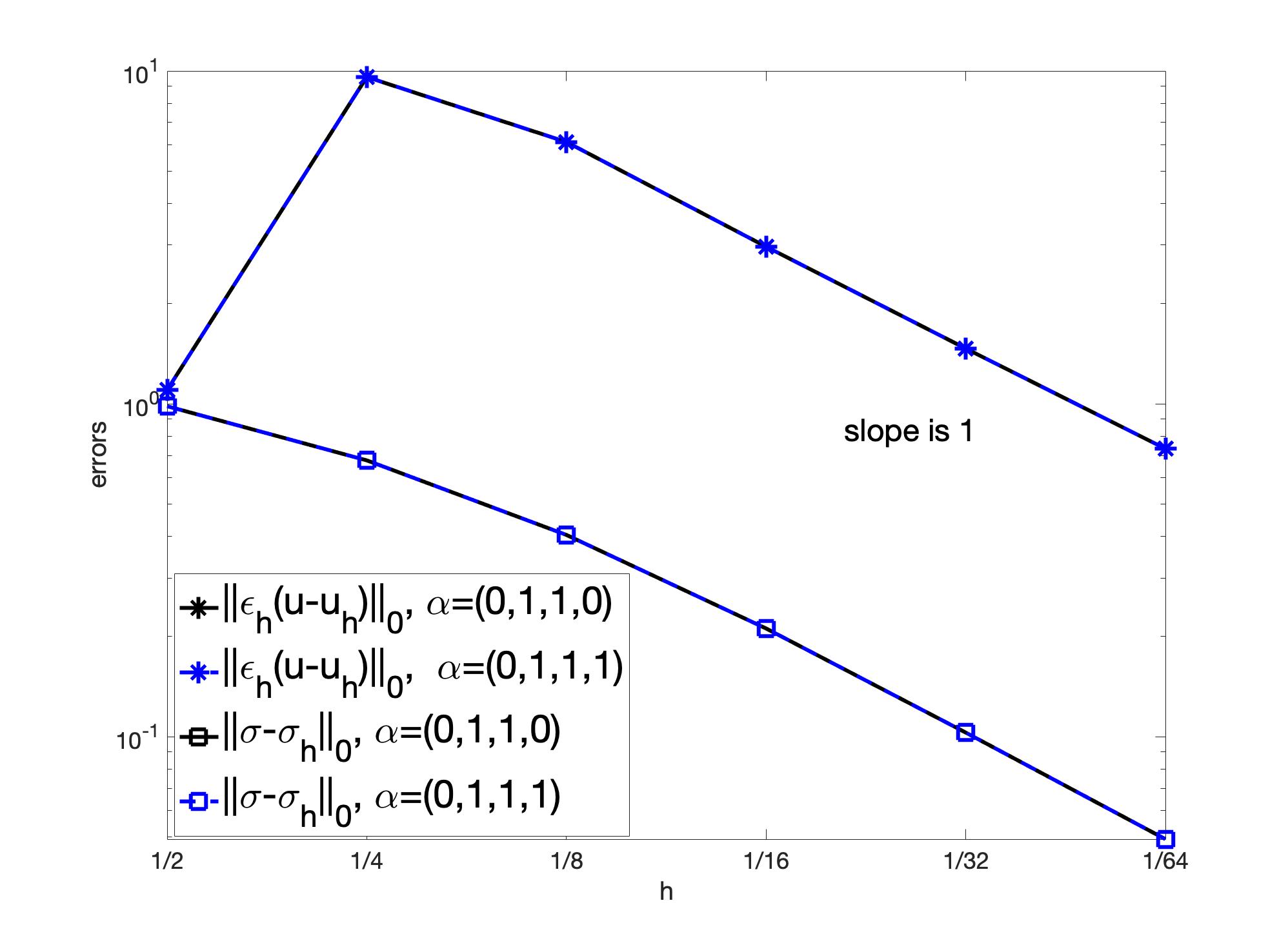
Figure 2: Errors of the lowest order $H^{1}$-based methods with $Q_{h}=Q_{h}^{\alpha_{1}}$, $V_{h}=V_{h}^{\alpha_{2}}$, $\check{Q}_{h}=\check{Q}_{h}^{\alpha_{3}}$, $\check{V}_{h}=\check{V}_{h}^{\alpha_{4}}$ and $\alpha=(\alpha_{1},\alpha_{2},\alpha_{3},\alpha_{4})$.

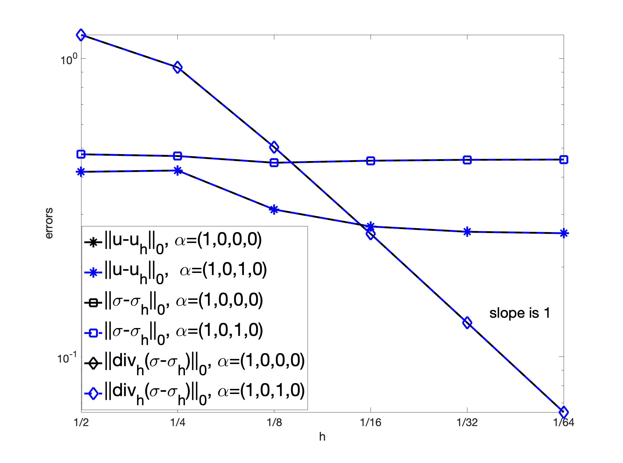
Figure 3: Errors of the lowest order $H({\rm div})$-based methods with $Q_{h}=Q_{h}^{\alpha_{1}}$, $V_{h}=V_{h}^{\alpha_{2}}$, $\check{Q}_{h}=\check{Q}_{h}^{\alpha_{3}}$, $\check{V}_{h}=\check{V}_{h}^{\alpha_{4}}$ and $\alpha=(\alpha_{1},\alpha_{2},\alpha_{3},\alpha_{4})$.

Figure 3 and 4 plot the errors of solutions for the lowest order $H({\rm div})$-based methods, which are new in literature. It is shown that the $H({\rm div})$-based methods with

$$Q_{h}=Q_{h}^{1},V_{h}=V_{h}^{0},\check{Q}_{h}=\check{Q}_{h}^{i},\check{V}_{h}=\check{V}_{h}^{0}\quad\mbox{with}\quad 0\leq i\leq 1$$ (109)

are not well-posed. Although the error $\|{\rm div}_{h}(\bm{\sigma}-\bm{\sigma}_{h})\|_{0}$ converges at the optimal rate $1.00$, the errors $\|\bm{\sigma}-\bm{\sigma}_{h}\|_{0}$ and $\|u-u_{h}\|_{0}$ do not converge at all. It also shows in Figure 3 and 4 that the new lowest order $H({\rm div})$-based methods with a larger space for $\check{V}_{h}$

$$Q_{h}=Q_{h}^{1},V_{h}=V_{h}^{0},\check{Q}_{h}=\check{Q}_{h}^{i},\check{V}_{h}=\check{V}_{h}^{1}\quad\mbox{with}\quad 0\leq i\leq 1$$ (110)

are well-posed and the corresponding errors $\|\bm{\sigma}-\bm{\sigma}_{h}\|_{0}$, $\|{\rm div}_{h}(\bm{\sigma}-\bm{\sigma}_{h})\|_{0}$ and $\|u-u_{h}\|_{0}$ admit the optimal convergence rate $1.00$. This coincides with the results in Theorem 3.2. The comparison between the $H({\rm div})$-based methods in (109) and (110) implies that Assumption (D2) is necessary for the wellposedness of the corresponding method.

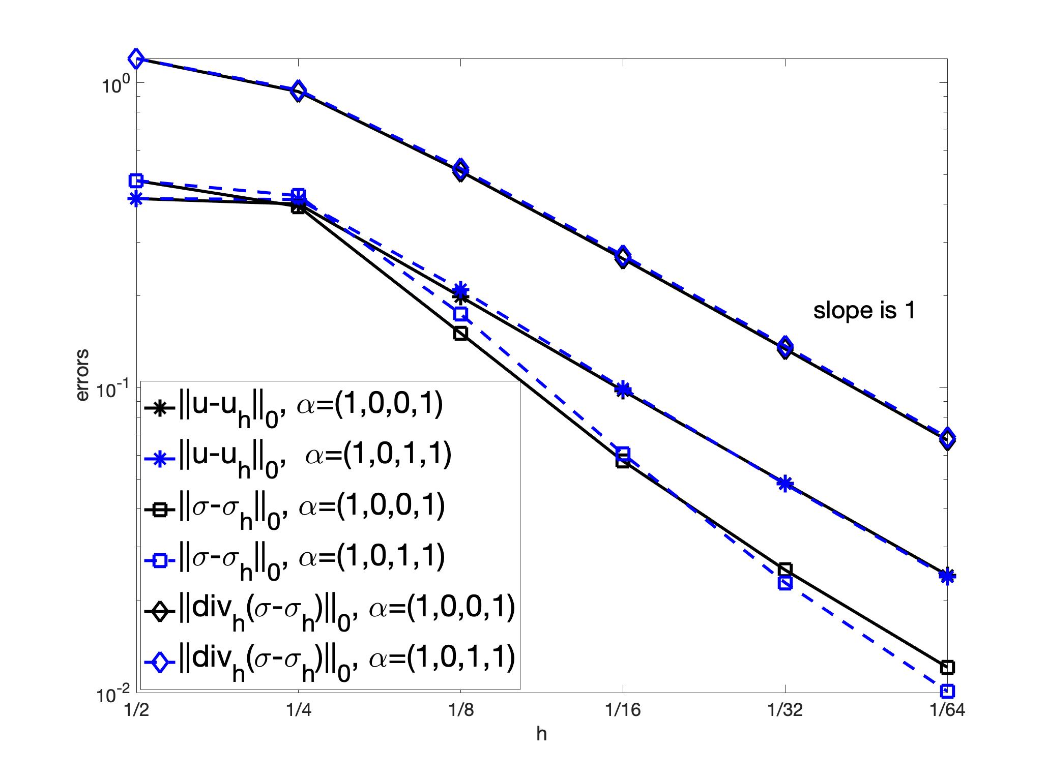
Figure 4: Errors of the lowest order $H({\rm div})$-based methods with $Q_{h}=Q_{h}^{\alpha_{1}}$, $V_{h}=V_{h}^{\alpha_{2}}$, $\check{Q}_{h}=\check{Q}_{h}^{\alpha_{3}}$, $\check{V}_{h}=\check{V}_{h}^{\alpha_{4}}$ and $\alpha=(\alpha_{1},\alpha_{2},\alpha_{3},\alpha_{4})$.

Figure 5: Errors for some high order $H({\rm div})$-based methods with $Q_{h}=Q_{h}^{\alpha_{1}}$, $V_{h}=V_{h}^{\alpha_{2}}$, $\check{Q}_{h}=\check{Q}_{h}^{\alpha_{3}}$, $\check{V}_{h}=\check{V}_{h}^{\alpha_{4}}$ and $\alpha=(\alpha_{1},\alpha_{2},\alpha_{3},\alpha_{4})$.

Consider the $L^{2}$ norm of the error of the stress tensor $\bm{\sigma}$. Figure 5 plots the errors for higher order $H({\rm div})$-based methods. For the XG formulation with $\alpha=(2,1,2,2)$, $k=1$ is less than $n=2$. Theorem 3.2 indicates that the convergence rate of $\|\bm{\sigma}-\bm{\sigma}_{h}\|_{0}$ is $2.00$ for this new second order $H({\rm div})$-based method, which is verified by the numerical results in Figure 5. For the XG formulation with $\alpha=(3,2,2,3)$, $k=n$ and the convergence rate of $\|\bm{\sigma}-\bm{\sigma}_{h}\|_{0}$ shown in Figure 5 is $4$, which coincides with the estimate in Theorem 3.3. This comparison indicates that the assumption $k\geq n$ in Theorem 3.3 is necessary and the error estimate of $\|\bm{\sigma}-\bm{\sigma}_{h}\|_{0}$ is optimal.

6.2 The lowest order methods with various $\nu$

Figure 6 plots the relative error of the approximate solutions of the $H^{1}$-based method with $Q_{h}^{0}\times\check{Q}_{h}^{1}\times V_{h}^{1}\times\check{V}_{h}^{0}$ with different $\nu$ ($\nu$ tends to $\frac{1}{2}$). Figure 6 shows that both $\|\epsilon_{h}(u-u_{h})\|_{0}$ and $\|\bm{\sigma}-\bm{\sigma}_{h}\|_{0}$ converge at the optimal rate 1.00, and the error $\|\bm{\sigma}-\bm{\sigma}_{h}\|_{0}$ are almost the same for different value of $\nu$.

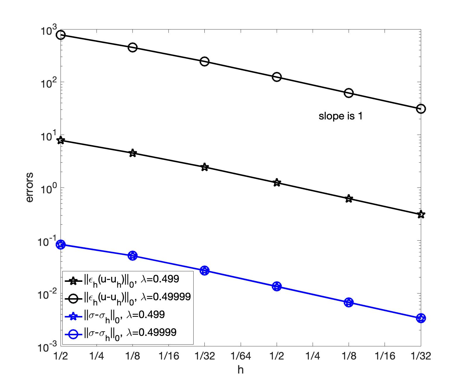
Figure 6: Errors for the lowest order $H^{1}$-based methods $Q_{h}^{0}\times\check{Q}_{h}^{1}\times V_{h}^{1}\times\check{V}_{h}^{0}$ with different $\nu$.

Figure 6 plots the relative error of the approximate solutions of the $H({\rm div})$-based method with $Q_{h}^{1}\times\check{Q}_{h}^{0}\times V_{h}^{0}\times\check{V}_{h}^{1}$ with different $\nu$ ($\nu$ tends to $\frac{1}{2}$). Figure 7 shows that the errors $\|u-u_{h}\|_{0}$, $\|\bm{\sigma}-\bm{\sigma}_{h}\|_{0}$ and $\|{\rm div}(\bm{\sigma}-\bm{\sigma}_{h})\|_{0}$ converge at the optimal rate 1.00, and the errors $\|\bm{\sigma}-\bm{\sigma}_{h}\|_{0}$ and $\|{\rm div}(\bm{\sigma}-\bm{\sigma}_{h})\|_{0}$ are almost the same as $\nu$ tends to $\frac{1}{2}$ which shows that the proposed schemes are locking-free.

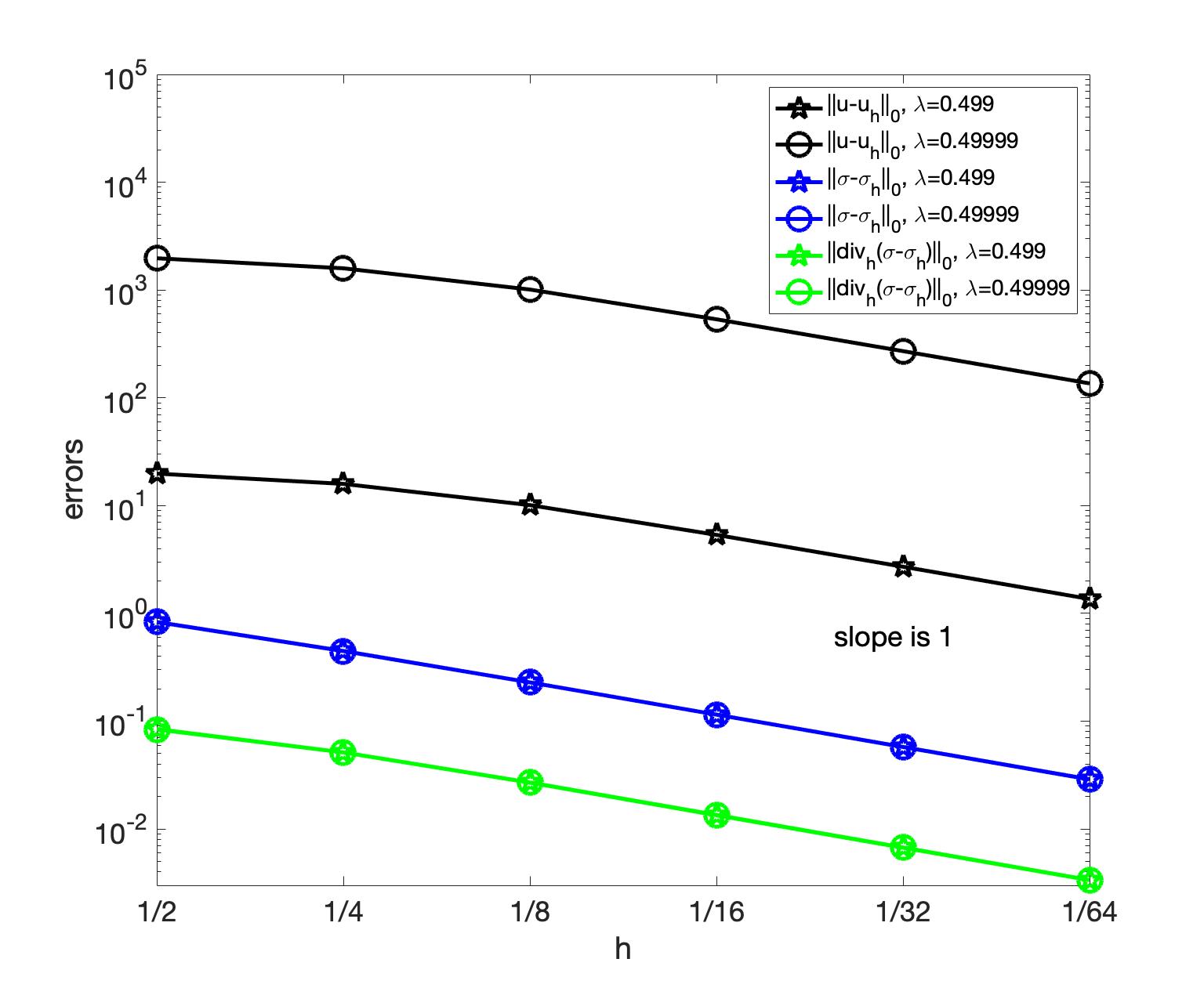
Figure 7: Errors for the lowest order $H({\rm div})$-based methods $Q_{h}^{1}\times\check{Q}_{h}^{0}\times V_{h}^{0}\times\check{V}_{h}^{1}$ with different $\nu$.

7 Conclusion

In this paper, a unified analysis of a four-field formulation is presented and analyzed for linear elasticity problem. This formulation is closely related to most HDG methods, WG methods, LDG methods and mixed finite elements in the literature. And some new methods are proposed following the unified framework. Some particular methods are proved to be hybridizable. In addition, uniform inf-sup conditions for the four-field formulation provide a unified way to prove the optimal error estimate under two different sets of assumptions. Also, these assumptions guide the design of some well-posed formulations new in literature.

References

- (1) Amara, M., Thomas, J.M.: Equilibrium finite elements for the linear elastic problem. Numerische Mathematik 33(4), 367–383 (1979)
- (2) Arnold, D., Awanou, G., Winther, R.: Finite elements for symmetric tensors in three dimensions. Mathematics of Computation 77(263), 1229–1251 (2008)
- (3) Arnold, D., Falk, R., Winther, R.: Mixed finite element methods for linear elasticity with weakly imposed symmetry. Mathematics of Computation 76(260), 1699–1723 (2007)
- (4) Arnold, D.N., Awanou, G., Winther, R.: Nonconforming tetrahedral mixed finite elements for elasticity. Mathematical Models and Methods in Applied Sciences 24(04), 783–796 (2014)
- (5) Arnold, D.N., Brezzi, F., Cockburn, B., Marini, L.D.: Unified analysis of discontinuous Galerkin methods for elliptic problems. SIAM journal on numerical analysis 39(5), 1749–1779 (2002)
- (6) Arnold, D.N., Brezzi, F., Douglas, J.: Peers: a new mixed finite element for plane elasticity. Japan Journal of Applied Mathematics 1(2), 347 (1984)
- (7) Arnold, D.N., Falk, R.S.: A new mixed formulation for elasticity. Numerische Mathematik 53(1-2), 13–30 (1988)
- (8) Arnold, D.N., Winther, R.: Mixed finite elements for elasticity. Numerische Mathematik 92(3), 401–419 (2002)
- (9) Arnold, D.N., Winther, R.: Nonconforming mixed elements for elasticity. Mathematical models and methods in applied sciences 13(03), 295–307 (2003)
- (10) Artioli, E., De Miranda, S., Lovadina, C., Patruno, L.: A stress/displacement virtual element method for plane elasticity problems. Computer Methods in Applied Mechanics and Engineering 325, 155–174 (2017)
- (11) Artioli, E., de Miranda, S., Lovadina, C., Patruno, L.: A family of virtual element methods for plane elasticity problems based on the Hellinger–Reissner principle. Computer Methods in Applied Mechanics and Engineering 340, 978–999 (2018)
- (12) Awanou, G.: A rotated nonconforming rectangular mixed element for elasticity. Calcolo 46(1), 49–60 (2009)
- (13) Boffi, D., Brezzi, F., Fortin, M.: Reduced symmetry elements in linear elasticity. Communications on Pure & Applied Analysis 8(1), 95–121 (2009)
- (14) Boffi, D., Brezzi, F., Fortin, M.: Mixed finite element methods and applications, vol. 44. Springer (2013)
- (15) Brezzi, F., Marini, L.D.: The three-field formulation for elasticity problems. GAMM-Mitteilungen 28(2), 124–153 (2005)
- (16) Brezzi, F., Marini, L.D.: Finite elements and virtual elements on classical meshes. Vietnam Journal of Mathematics pp. 1–29 (2021)
- (17) Chen, G., Xie, X.: A robust weak Galerkin finite element method for linear elasticity with strong symmetric stresses. Computational Methods in Applied Mathematics 16(3), 389–408 (2016)
- (18) Chen, L., Hu, J., Huang, X.: Stabilized mixed finite element methods for linear elasticity on simplicial grids in . Computational Methods in Applied Mathematics 17(1), 17–31 (2017)
- (19) Chen, Y., Huang, J., Huang, X., Xu, Y.: On the local discontinuous Galerkin method for linear elasticity. Mathematical Problems in Engineering (2010)
- (20) Cockburn, B., Karniadakis, G.E., Shu, C.W.: The development of discontinuous Galerkin methods. In: Discontinuous Galerkin Methods, pp. 3–50. Springer (2000)
- (21) Courant, R.: Variational methods for the solution of problems of equilibrium and vibrations. Lecture Notes in Pure and Applied Mathematics (1994)
- (22) Da Veiga, L.B., Brezzi, F., Marini, L.D.: Virtual elements for linear elasticity problems. SIAM Journal on Numerical Analysis 51(2), 794–812 (2013)
- (23) Dassi, F., Lovadina, C., Visinoni, M.: A three-dimensional Hellinger–Reissner virtual element method for linear elasticity problems. Computer Methods in Applied Mechanics and Engineering 364, 112910 (2020)
- (24) Eastwood, M.: A complex from linear elasticity. In: Proceedings of the 19th Winter School ” Geometry and Physics”, pp. 23–29. Circolo Matematico di Palermo (2000)
- (25) Feng, K.: Finite difference schemes based on variational principles. Applied Mathematics and Computational Mathematics 2, 238–262 (1965)
- (26) Fu, G., Cockburn, B., Stolarski, H.: Analysis of an HDG method for linear elasticity. International Journal for Numerical Methods in Engineering 102(3-4), 551–575 (2015)
- (27) Gatica, G.N., Sequeira, F.A.: Analysis of an augmented hdg method for a class of quasi-newtonian stokes flows. Journal of Scientific Computing 65(3), 1270–1308 (2015)
- (28) Gong, S., Wu, S., Xu, J.: New hybridized mixed methods for linear elasticity and optimal multilevel solvers. Numerische Mathematik 141(2), 569–604 (2019)
- (29) Gopalakrishnan, J., Guzmán, J.: Symmetric nonconforming mixed finite elements for linear elasticity. SIAM Journal on Numerical Analysis 49(4), 1504–1520 (2011)
- (30) Hansbo, P., Larson, M.G.: Discontinuous Galerkin and the Crouzeix–Raviart element: application to elasticity. ESAIM: Mathematical Modelling and Numerical Analysis 37(1), 63–72 (2003)
- (31) Hong, Q., Hu, J., Shu, S., Xu, J.: A discontinuous Galerkin method for the fourth-order curl problem. Journal of Computational Mathematics 30(6), 565–578 (2012)
- (32) Hong, Q., Kraus, J.: Uniformly stable discontinuous Galerkin discretization and robust iterative solution methods for the Brinkman problem. SIAM Journal on Numerical Analysis 54(5), 2750–2774 (2016)
- (33) Hong, Q., Kraus, J.: Parameter-robust stability of classical three-field formulation of BIOT’s consolidation model. Electronic Transactions on Numerical Analysis 48, 202–226 (2018)
- (34) Hong, Q., Kraus, J., Lymbery, M., Philo, F.: Conservative discretizations and parameter-robust preconditioners for Biot and multiple-network flux-based poroelasticity models. Numerical Linear Algebra with Applications 26(4), e2242 (2019)
- (35) Hong, Q., Kraus, J., Xu, J., Zikatanov, L.: A robust multigrid method for discontinuous Galerkin discretizations of Stokes and linear elasticity equations. Numerische Mathematik 132(1), 23–49 (2016)
- (36) Hong, Q., Li, Y., Xu, J.: An extended Galerkin analysis in finite element exterior calculus. arXiv preprint arXiv:2101.09735 (2021)
- (37) Hong, Q., Wang, F., Wu, S., Xu, J.: A unified study of continuous and discontinuous Galerkin methods. Science China Mathematics 62(1), 1–32 (2019)
- (38) Hong, Q., Wu, S., Xu, J.: An extended Galerkin analysis for elliptic problems. Science China Mathematics pp. 1–18 (2020)
- (39) Hong, Q., Xu, J.: Uniform stability and error analysis for some discontinuous Galerkin methods. Journal of Computational Mathematics 39(2), 283–310 (2020)
- (40) Hrennikoff, A.: Solution of problems of elasticity by the framework method. Journal of Applied Mechanics 8(4), A169–A175 (1941)
- (41) Hu, J.: Finite element approximations of symmetric tensors on simplicial grids in : The higher order case. Journal of Computational Mathematics 33(3), 283–296 (2015)
- (42) Hu, J., Ma, R.: Nonconforming mixed finite elements for linear elasticity on simplicial grids. Numerical Methods for Partial Differential Equations 35(2), 716–732 (2019)
- (43) Hu, J., Shi, Z.C.: Lower order rectangular nonconforming mixed finite elements for plane elasticity. SIAM Journal on Numerical Analysis 46(1), 88–102 (2007)
- (44) Hu, J., Zhang, S.: A family of conforming mixed finite elements for linear elasticity on triangular grids. arXiv preprint arXiv:1406.7457 (2014)
- (45) Hu, J., Zhang, S.: A family of symmetric mixed finite elements for linear elasticity on tetrahedral grids. Science China Mathematics 58(2), 297–307 (2015)
- (46) Hu, J., Zhang, S.: Finite element approximations of symmetric tensors on simplicial grids in : The lower order case. Mathematical Models and Methods in Applied Sciences 26(9), 1649–1669 (2016)
- (47) Man, H., Hu, J., Shi, Z.C.: Lower order rectangular nonconforming mixed finite element for the three-dimensional elasticity problem. Mathematical Models and Methods in Applied Sciences 19(01), 51–65 (2009)
- (48) Pechstein, A., Schöberl, J.: Tangential-displacement and normal–normal-stress continuous mixed finite elements for elasticity. Mathematical Models and Methods in Applied Sciences 21(08), 1761–1782 (2011)
- (49) Pechstein, A.S., Schöberl, J.: An analysis of the TDNNS method using natural norms. Numerische Mathematik 139(1), 93–120 (2018)
- (50) Qiu, W., Shen, J., Shi, K.: An HDG method for linear elasticity with strong symmetric stresses. Mathematics of Computation 87(309), 69–93 (2018)
- (51) Soon, S.: Hybridizable discontinuous Galerkin method for solid mechanics. Ph.D. thesis, University of Minnesota (2008)
- (52) Soon, S., Cockburn, B., Stolarski, H.: A hybridizable discontinuous Galerkin method for linear elasticity. International journal for numerical methods in engineering 80(8), 1058–1092 (2009)
- (53) Stein, E., Rolfes, R.: Mechanical conditions for stability and optimal convergence of mixed finite elements for linear plane elasticity. Computer methods in applied mechanics and engineering 84(1), 77–95 (1990)
- (54) Stenberg, R.: On the construction of optimal mixed finite element methods for the linear elasticity problem. Numerische Mathematik 48(4), 447–462 (1986)
- (55) Stenberg, R.: A family of mixed finite elements for the elasticity problem. Numerische Mathematik 53(5), 513–538 (1988)
- (56) Stenberg, R.: Two low-order mixed methods for the elasticity problem. The mathematics of finite elements and applications, VI (Uxbridge, 1987) pp. 271–280 (1988)
- (57) Fraeijs de Veubeke, B.: Stress function approach. Proc. of the World Congress on Finite Element Methods in Structural Mechanics. Vol. 1, Bournemouth, Dorset, England pp. J.1–J.51 (1975)
- (58) Wang, C., Wang, J., Wang, R., Zhang, R.: A locking-free weak Galerkin finite element method for elasticity problems in the primal formulation. Journal of Computational and Applied Mathematics 307, 346–366 (2016)
- (59) Wang, F., Wu, S., Xu, J.: A mixed discontinuous Galerkin method for linear elasticity with strongly imposed symmetry. Journal of Scientific Computing 83(1), 1–17 (2020)
- (60) Wang, R., Wang, X., Zhang, K., Zhou, Q.: Hybridized weak Galerkin finite element method for linear elasticity problem in mixed form. Frontiers of Mathematics in China 13(5), 1121–1140 (2018)
- (61) Wang, R., Zhang, R.: A weak Galerkin finite element method for the linear elasticity problem in mixed form. Journal of Computational Mathematics 36(4), 469–491 (2018)
- (62) Wu, S., Gong, S., Xu, J.: Interior penalty mixed finite element methods of any order in any dimension for linear elasticity with strongly symmetric stress tensor. Mathematical Models and Methods in Applied Sciences 27(14), 2711–2743 (2017)
- (63) Yi, S.Y.: Nonconforming mixed finite element methods for linear elasticity using rectangular elements in two and three dimensions. Calcolo 42(2), 115–133 (2005)
- (64) Yi, S.Y.: A new nonconforming mixed finite element method for linear elasticity. Mathematical Models and Methods in Applied Sciences 16(07), 979–999 (2006)
- (65) Yi, S.Y.: A lowest-order weak Galerkin method for linear elasticity. Journal of Computational and Applied Mathematics 350, 286–298 (2019)