The impact of electron-electron correlation in ultrafast attosecond single ionization dynamics

Abstract

The attosecond ultrafast ionization dynamics of correlated two- or many-electron systems have, so far, been mainly addressed investigating atomic systems. In the case of single ionization, it is well known that electron-electron correlation modifies the ionization dynamics and observables beyond the single active electron picture, resulting in effects such as the Auger effect or shake-up/down and knock-up/down processes. Here, we extend these works by investigating the attosecond ionization of a molecular system involving correlated two-electron dynamics, as well as non-adiabatic nuclear dynamics. Employing a charge-transfer molecular model system with two differently bound electrons, a strongly and a weakly bound electron, we distinguish different pathways leading to ionization, be it direct ionization or ionization involving elastic and inelastic electron scattering processes. We find that different pathways result in a difference in the electronic population of the parent molecular ion, which, in turn, involves different subsequent (non-adiabatic) postionization dynamics on different time scales.

I Introduction

For many elementary processes in multi-electron systems, such as in photoionization, electron-impact ionization, the Auger effect, and other radiative processes, the impact of correlated electron-electron dynamics plays a crucial role [1]. In the case of ionization, these electron correlations affect the state and the dynamics of the residual cation on an atto- and femtosecond timescale. As a consequence, the remaining bound electron(s) can be excited (shake-up/knock-up processes [2]), relaxed (shake-down/knock-down), or even ejected subsequently (Auger process) [3]. Such time-resolved ionization dynamics of multi-electron systems have been investigated in various theoretical and experimental studies, for a review see for example Ref. 4.

On the experimental side, the advent of ultrashort femto- or even attosecond pulses in the extreme ultraviolet (XUV) regime being available either via table-top high-order harmonic generation or the newest generation of (X)FEL sources, for example, paved the way for the observation of these processes in real time, e.g. employing the attosecond streaking technology [5, 6, 7, 8, 9]. However, resolving the details of these complex correlated many-body phenomena involving nuclear and electronic degrees of freedom still poses a challenge for computational simulations.

Most of the theoretical work has been focused on the helium atom as the simplest two-electron system [10, 9, 11, 2]. Effects which have been examined are the Wigner-Smith time delay and electron-electron correlation under the influence of an (infrared) laser field in the context of streaking spectroscopy [4, 11, 2, 12, 13]. For molecules, the physics becomes even more complex, also due to the multi-scatterer nature compared to the centrosymmetric atoms. Ning et al. have investigated the simplest, prototypical molecule, H${}_{2}^{+}$, and found pronounced interference effects (Cohen-Fano interferences, [14]) caused by the two scattering centers [15]. However, this prototype case inherently does not involve any multi-electron effects. Other molecular systems investigated theoretically include endohedral complexes of type A@C₆₀ [16, 17] or, employing multi-configurational approaches, ionization and subsequent charge migration of small amino acids [18, 19, 20, 21, 22, 23]. A few works have considered both, the correlated electron dynamics and the nuclear motion [24, 25, 26, 27].

In order to reduce computational costs, numerical simulations commonly employ approximations such as the sudden approximation, frozen nuclear degrees of freedom, or the single-active electron approximation [28]. Within the framework of the latter, one assumes that the dynamics of the active electrons is sufficiently fast so that the "inactive" electrons do no adapt within its time scale, i.e. no electron correlated dynamics occurs. However, it has been shown by Awasthi et al. that electron correlation even upon XUV- or X-ray-induced ionization of multi-electron systems plays an important role and cannot be neglected [29, 30].

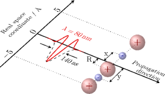
Figure 1: Configuration of the extended Shin-Metiu system: An ultrashort XUV pulse is used to ionize a linear molecule aligned with the pulse’s polarization axis. The molecule consists of two fixed nuclei at $\pm 5$ Å, two mobile electrons with coordinates $x$ and $y$, and a movable central nucleus at $R$. The mobile nucleus is initially localized at negative $R$ values, whereas the two electrons reside on both sides. Thus, in the electronic ground state, the electron at negative coordinates is stronger bound than the electron located at positive values.

In this work, we investigate the effects of such electron-electron correlation as well as non-adiabatic effects on the postionization dynamics of a molecular charge transfer model system in a time-resolved picture. Moreover, we aim to thoroughly distinguish the processes contributing to the electron-nuclear post-ionization dynamics. The model system, which has been originally suggested by Shin and Metiu [31, 32], has been extended by the group of Engel to include two electrons [33, 34]. This system, which will be introduced in more detail in Sec. II, possesses, due to asymmetric initial conditions, one stronger and one weaker bound electron with anti-parallel spin. Interaction with an attosecond XUV pulse leads to the emission of one electron. We show that several processes occur on different timescales which have an impact on the electronic configuration of the residual molecular ion: (a) direct photoemission of either the weaker or the stronger bound electron, without passing the respective other electron, yet, affecting its quantum state due to an altered electrostatic environment (shake-up/shake-down processes); (b) emission processes, where upon photoabsorption, the accelerated electron needs to ”pass“ the other electron. The latter process involves an immediate electron-electron interaction, which leads to both, inelastic and elastic scattering. As a result, the second electron is either excited into higher bound states (knock-up), relaxed into lower states (knock-down) [2], or adopts the momentum of the electron originally accelerated by the electric field and is emitted in its stead (”indirect“ photoemission); and (c) non-adiabatic transition processes during the postionization dynamics.

The paper is organized as follows: After a short description of the model and the numerical methods utilized in Sec. II, we will present the different pathways, analyzed additionally with the help of desymmetrized wave functions and restricted interactions of the electrons with the external electric field. The resulting dynamics is discussed by means of the final state-dependence in the residual ion in Sec. III. The paper ends with a summary and conclusion in Sec. IV.

II Theory

II.1 The full model system

The model we apply in this work represents an extension to the one originally suggested by Shin and Metiu [31, 32]. In their work, a linear, one-dimensional charge-transfer model system was employed consisting of two fixed nuclei with charges $Z_{1}$ and $Z_{2}$ at the positions $\pm L$/2, one moving nucleus ($Z$) in between with coordinate $R$, and one electron, here with coordinate $y$, giving rise to the potential:

$$V^{\text{1e}}(y,R )={}\frac{e^{2}}{4\pi\epsilon_{0}}\left[\frac{Z_{1}Z}{|L/2-R|}\!+\!\frac{Z_{2}Z}{|L/2+R|}\!-\!\frac{Z\>\text{erf}(|R-y|/R_{c})}{|R-y|}\right.$$

$$- \left.\frac{Z_{1}\>\text{erf}(|L/2-y|/R_{f})}{|L/2-y|}-\frac{Z_{2}\>\text{erf}(|L/2+y|/R_{f})}{|L/2+y|}\right],$$ (1)

where the error functions (erf) describe a truncated Coulomb interaction between individual particles. The truncation parameters $R_{f}$ and $R_{c}$ specify the interaction strength between the electron and the fixed nuclei and the mobile nucleus, respectively [31, 32].

Here, we use an extension to this model introduced by Engel and coworkers, where a second electron, $x$, is added to the system [33, 34]. The whole particle configuration is shown in Fig. 1. The system’s potential takes on the form

$$V^{\mathrm{2e}}(x,y,R)={} V^{\mathrm{1e}}(y,R)+\frac{e^{2}}{4\pi\epsilon_{0}}\left[-\frac{Z\>\text{erf}(|R-x|/R_{c})}{|R-x|}\right.$$

$$-\frac{Z_{1}\>\text{erf}(|L/2-x|/R_{f})}{|L/2-x|}-\frac{Z_{2}\>\text{erf}(|L/2+x|/R_{f})}{|L/2+x|}$$

$$\left.+\frac{\text{erf}(|x-y|/R_{e})}{|x-y|}\right],$$ (2)

where $R_{e}$ scales the electron-electron interaction [35, 36, 37, 34, 38, 39, 35, 40]. The fixed nuclei have a distance of $L=10$ Å. Nuclear charges are $Z=Z_{1}=Z_{2}=1$. All truncation parameters have been set to $R_{f}=R_{c}=R_{e}=1.5$ Å, corresponding to the weak-coupling regime [38].

The three particle configuration of the model and its dynamics can be fully solved numerically. However, for interpretation, we calculate for the one-electron (1e) and the two-electron (2e) systems the (adiabatic) electronic eigenfunctions, $\varphi^{\text{1e}}_{n}(y;R)$ and $\varphi^{\text{2e}}_{n}(x,y;R)$, with eigenvalues $V^{\text{1e}}_{n}(R)$ and $V^{\text{2e}}_{n}(R)$, respectively, by solving the following eigenvalue equations:

$$\left[\frac{p_{y}^{2}}{2m_{e}}+{V}^{\mathrm{1e}}(y,R)\right]\varphi^{\text{1e}}_{n}(y;R)={} V^{\text{1e}}_{n}(R)\,\varphi^{\text{1e}}_{n}(y;R)$$ (3)

$$\left[\frac{p_{x}^{2}}{2m_{e}}+\frac{p_{y}^{2}}{2m_{e}}+{V}^{\mathrm{2e}}(x,y,R)\right] \varphi^{\text{2e}}_{n}(x,y;R)={}$$

$$V^{\text{2e}}_{n}(R)\,\varphi^{\text{2e}}_{n}(x,y;R),$$ (4)

where $m_{e}$ is the electron mass and $p_{x}$ and $p_{y}$ refer to the electronic momenta. For the two-electron case, the wavefunctions are symmetrized according to Pauli’s principle and correspond to an anti-parallel spin configuration. The obtained potential energy curves, $V_{n}^{1e/2e}(R)$, are shown in Fig. 2a for one (upper panel) and two bound electrons (bottom panel). The one-electron model will be used to analyze the postionization dynamics of one ($y$) electron remaining in the parent ion after removal of the other ($x$) electron upon ionization. The first five electronic eigenfunctions of the single electron model, $\varphi_{n}^{\text{1e}}(y;R_{0})$, are shown in Fig. 2b for an asymmetric nuclear configuration, $R_{0}=-2.05$ Å, corresponding to the system initialization (see below). Note, that among these states, for $n=0,1$, and 3, the electron is mostly localized on the left-hand side ($y<0$), i.e. at the two close nuclei (in a strongly bound location), whereas for $n=2$ and 4 it is predominantly located at the right hand side ($y>0$), i.e. at the single nucleus (weakly bound).

The system interacts with an ultrashort attosecond XUV pulse which, using the dipole approximation and velocity gauge, results in the Hamiltonian:

$${\mathcal{H}}(t)={} \frac{{P}^{2}}{2M}+\frac{{p}_{x}^{2}}{2m_{e}}+\frac{{p}_{y}^{2}}{2m_{e}}+V^{\mathrm{2e}}(x,y,R)$$

$$+e\,\mathcal{A}(t)\left(-\frac{Z}{M}{P}+\frac{p_{x}}{m_{e}}+\frac{p_{y}}{m_{e}}\right),$$ (5)

where $M$ is the proton mass and $P$ the nuclear momentum. The electric field of the ultrashort ionizing XUV pulse is described via its vector potential $\mathcal{A}(t)$ with a polarization along the molecular axis:

$$\mathcal{A}(t)=-\frac{E_{0}}{\omega}\,g(t-T)\,\sin\big(\omega(t-T)+\phi\big{missing}).$$ (6)

Here, $E_{0}=-8.7$ V/Å (or -0.169 a.u.) is the electric field strength (corresponding to an intensity of 1.0$\times 10^{15}$ W/cm²), $\omega$ the field’s angular frequency, and $g(t-T)$ a Gaussian pulse envelope function centered around $T=0$ fs with a full-width half-maximum (FWHM) of $140$ as (2.894 a.u.). The angular frequency corresponds to a wavelength of $\lambda=80$ nm ($\hat{=}\;15.5$ eV or 0.570 a.u.), which is sufficient to singly ionize the molecule through single photon absorption, see Fig. 2a. The spectral width of the attosecond pulse intensity is 18.4 eV (0.676 a.u.). The carrier-envelope phase (CEP) $\phi$ is set to zero, corresponding to a sine-shaped vector potential or an approximately cosine-shaped electric field.

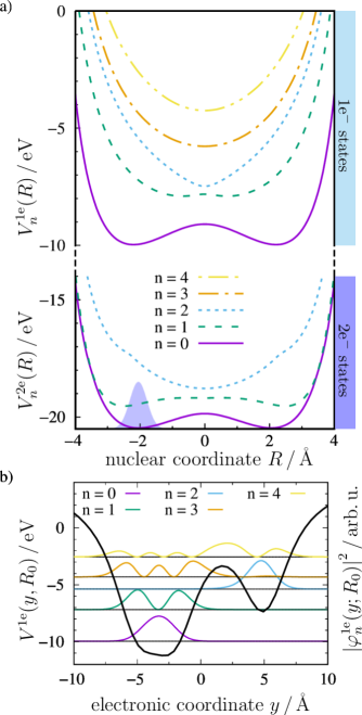
Figure 2: (a) Potential energy curves $V^{\text{1e,2e}}_{n}(R)$ for the lowest electronic eigenstates $\varphi^{\text{1e,2e}}_{n}$ of the one-electron (1e) and two-electron (2e) systems. The blue-shaded area depicts the initial nuclear wave packet $\chi(R)$ centered around the minimum at $R_{0}=-2.05\,\text{\AA{}}$.
(b) Potential energy $V^{\mathrm{1e}}(y,R_{0})$ (solid black line) and first five electronic eigenfunctions of the single-electron system, $\left|\varphi^{\text{1e}}_{n}(y;R_{0})\right|^{2}$, at the initial, near-equilibrium nuclear geometry $R_{0}$.

II.2 Propagation and initialization

The full system’s wave function $\Psi(x,y,R,t)$ is represented on a three-dimensional grid with a range of [-240, 240] Å with 1024 grid points in $x$- and $y$-direction, respectively, and of [-4.99, 4.99] Å with 128 points along the $R$-direction. The time-dependent Schrödinger equation for the Hamiltonian defined in Eq. (5) is solved numerically with a timestep of 5 as using the split-operator technique [41] and the FFTW 3 library [42] for Fourier transforms. For the details on the numerics please see our previous publications, e.g. Ref. 38. The simulation starts at $t_{0}=-4$ fs, well before the XUV pulse enters the system. Reflection at the grid boundaries is suppressed by multiplying $\Psi(x,y,R,t)$ at each timestep with a splitting function [43]

$$f(x,y)={} \big{[}1+\mathrm{e}^{\zeta_{1}\,(|x|-\zeta_{2})}\big{]}^{-1}\,\big{[}1+\mathrm{e}^{\zeta_{1}\,(|y|-\zeta_{2})}\big{]}^{-1}$$ (7)

with the parameters $\zeta_{1}=5.67$ Å^-1 and $\zeta_{2}=235$ Å.

II.2.1 Full fermionic wave function

The initial state is assumed to be a product state of the two-electron adiabatic electronic ground state, $\varphi_{0}^{\mathrm{2e}}(x,y;R)$, and a nuclear wave function

$$\Psi(x,y,R,t_{0})=\varphi_{0}^{\mathrm{2e}}(x,y;R)\,\chi(R).$$ (8)

The adiabatic electronic eigenstates are obtained by solving the field-free electronic Schrödinger equations, Eqs. (3) and (4), via the relaxation method [44].

The nuclear part of the initial wave function, $\chi(R)$, is assumed to be a Gaussian-shaped vibrational wave packet centered around the left local minimum of the double-well potential at $R_{0}\!=\!-2.05$ Å (see shaded area in Fig. 2a):

$$\chi(R)=N_{0}\,e^{-\beta_{R}(R-R_{0})^{2}}.$$ (9)

Here, $N_{0}$ serves as normalization constant and the width $\beta_{R}\!=\!7.14$ Å^-2. This way, the Gaussian closely resembles the left-hand side of the vibrational ground state eigenfunction, which is symmetric around $R=0$. We note that the factorized, asymmetric initial state does not correspond to the total ground state of the system. It rather corresponds to one of two energetically equal realizations. This is a common situation, where the system resides in one potential well as encountered, for example, in NH₃ inversion or isomerization processes.

The initial two-electron densities, i. e. $\int|\Psi(x,y,R,t_{0})|^{2}\,\mathrm{d}R$, is displayed in the top layer of Fig. 3. Note that cuts through the spatial distribution of the electronic part – given by the two-electron groundstate wavefunction $\varphi^{\text{2e}}_{0}(x,y;R)$ – approximately correspond to the one-electron functions $\varphi^{1e}_{0}(y;R)$ and $\varphi^{1e}_{2}(y;R)$. The simulation results obtained for these initial conditions (and their relation to the one-electron electronic eigenfunctions) are discussed in Sec. III.1. Please note that as we neglect any spin-dependent interaction, spin and spatial coordinates factorize. We therefore only consider the (symmetric) spatial part of the full wave function.

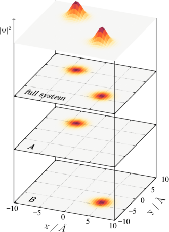
Figure 3: Initial two-electron densities, $\int|\Psi(x,y,R,t_{0})|^{2}\,\mathrm{d}R$, entering the propagation. Top plane: fully symmetric spatial wave function calculated via the relaxation method. Descending from top to bottom: Projection onto the 2D plane of the full system and the artificial subsystems, (A) and (B), respectively.

II.2.2 Artificial subsystems with distinguishable electrons

For analysis purposes, the full wave function, Eq. (8), is partitioned into two desymmetrized subsystems with

$$\text{(A)~{}~{}}\psi_{A}(x,y,R,t_{0})\equiv{} \sqrt{2}\,\Psi(x,y,R,t_{0})\,\Theta(y-x),$$ (10a)

$$\text{(B)~{}~{}}\psi_{B}(x,y,R,t_{0})\equiv{} \sqrt{2}\,\Psi(x,y,R,t_{0})\,\Theta(x-y),$$ (10b)

respectively (Fig. 3, lower panels). In above equation, $\Theta(x)$ is the Heaviside step function. These partial wave functions each describing one half of the full system, split along the $x\!=\!y$-diagonal. By doing so, the wave functions $\psi_{A}(x,y,R,t_{0})$ and $\psi_{B}(x,y,R,t_{0})$ vaguely resemble a wave function in Hartree-product form, because now $x$ and $y$ effectively describe identical, yet distinguishable electrons. In the initial configuration of subsystem A (B) the $x$ ($y$) electron is strongly bound (with an approximate binding energy of $E_{B}^{\text{strong}}=V^{\mathrm{1e}}_{2}(R_{0})-V^{\mathrm{2e}}_{0}(R_{0})=15.1$ eV), whereas the $y$ ($x$) electron ($E_{B}^{\text{weak}}=V^{\mathrm{1e}}_{0}(R_{0})-V^{\mathrm{2e}}_{0}(R_{0})=10.5$ eV) is weakly bound. Technically, the abrupt cut-off of the wavefunction leads to a weak field-free ionization signal. This background signal is removed from the propagated wave function until $t=-250$ as, i.e. before the ionizing XUV pulse interacts with the system, by truncating $\Psi(x,y,R,t\leq-250\,\text{as})$ through multiplication with $\Theta(25\,\text{\AA{}}-\absolutevalue{x})\,\Theta(25\,\text{\AA{}}-\absolutevalue{y})$. The different ionization pathways revealed by these subsystems’ dynamics are discussed in Sec. III.2.

II.2.3 Restricted field interaction

For analysis, further disentanglement of individual ionization pathways and their underlying intramolecular dynamics is achieved by artificially restricting the field interaction. To this end, simulations on subsystems A and B are performed with the modified Hamiltonian

$${\mathcal{H}}^{\prime}(t)={} \frac{{P}^{2}}{2M}+\frac{{p}_{x}^{2}}{2m_{e}}+\frac{{p}_{y}^{2}}{2m_{e}}+V^{\mathrm{2e}}(x,y,R)$$

$$+e\,\mathcal{A}(t)\left(-\frac{Z}{M}{P}+\frac{p_{\xi}}{m_{e}}\right),$$ (11)

where $\xi\in\{x,y\}$ refers to either the $x$ or the $y$ electron. Thus, field interaction is limited to a specific electron. This restriction allows us to distinguish direct and electron correlation driven photoionization pathways. Obtained results are presented and discussed in Sec. III.3.

II.3 Identification of single ionization

To isolate fractions of the wave functions that belong to the singly ionized system, the photoelectron dynamics are devined via the ionization signal in regions far from the molecule using the mask function

$$c(x,y)=c_{x}(x)\cdot\big{[}1-c_{y}(y)\big{]}$$ (12)

with

$$c_{\xi}(\xi)=\begin{cases}0&\text{if }0~{}<~{}\lvert\xi\rvert\leq\xi_{c}\\ \sin^{2}\big{(}\frac{\lvert\xi\rvert-\xi_{c}}{\Delta\xi}\frac{\pi}{2}\big{)}&\text{if }\xi_{c}<\lvert\xi\rvert\leq\xi_{c}\!+\!\Delta\xi\\ 1&\text{if }\xi_{c}\!+\!\Delta\xi<\lvert\xi\rvert\leq\xi_{\mathrm{end}}\end{cases},$$ (13)

where $\xi\in\{x,y\}$ with corresponding $x_{c}=y_{c}=25$ Å, $\Delta x=\Delta y=10\,$Å, and $x_{\mathrm{end}}=y_{\mathrm{end}}=240\,$Å marking the end points of the simulation grid. As a result, the mask $c(x,y)$ selects parts of the electronic wave functions

$$\psi_{\text{out}}(x,y,R,t)\equiv c(x,y)\,\psi(x,y,R,t)$$ (14)

at large $x$ and low $y$ coordinates, corresponding to the emission of the $x$ electron, whereas the other ($y$) electron remains bound at the parent molecular ion. Due to symmetry in the electronic coordinates, it is sufficient to only evaluate signals along the $x$ direction. Note, that this mask is independent of $R$, as the nuclear part of the wave function remains well confined between the two outer nuclei. Further segmentation of $\psi_{\text{out}}(x,y,R,t)$ into subregions $S$ will be introduced in Sec. III.1.

III Results and Discussion

III.1 Fully correlated fermionic wave function

Interaction of the initial state with the ultrashort XUV pulse induces electron dynamics within the (non-ionized) two-electron system and leads to single ionization. While for atomic systems, an ionization signal can be extracted via projection of the wave function onto a set of Coulomb waves [11], such an approach is not feasible for the multi-centered potential of the molecular model employed here. Instead, we remove the two-electron components for the first 35 two-electron states, for which both electrons are bound, from the total wavefunction. Then we project the remainder (containing only a single bound electron) onto the basis spanned by the electronic eigenfunctions $\{\varphi_{n}^{\text{1e}}(y;R)\}$ of the one-electron system [2]:

$$P_{n}(t)={}\iint\left|{\int\varphi^{\text{1e}}_{n}(y;R)\,\Psi^{\text{1e}}(x,y,R,t)~{}\mathrm{d}y}\right|^{2}\mathrm{d}x~{}\mathrm{d}R,$$ (15)

using the following defintions:

$$\Psi^{\text{1e}}(x,y,R,t)\equiv{}\Psi(x,y,R,t)-\sum_{m=0}^{34}a^{\text{2e}}_{m}(t)\,\varphi^{\text{2e}}_{m}(x,y;R),$$ (16)

$$a^{\text{2e}}_{m}(t)\equiv{}\iiint{\varphi^{\text{2e}}_{m}(x,y;R)\,\Psi(x,y,R,t)~{}\mathrm{d}x}~{}\mathrm{d}y~{}\mathrm{d}R.$$ (17)

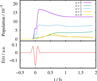
Figure 4: Population of the single-electron states upon projection onto the basis spanned by $\{\varphi_{n}^{\mathrm{1e}}(y;R)\}$ after removal of all two-electron states (upper panel) and temporal profile of the XUV pulse’s electric field (lower panel).

The populations $P_{n}(t)$ are shown in Fig. 4 upper panel. Note, that in the basis considered here, only contributions are obtained, where the $y$ electron remains bound, while the $x$ electron is ejected. Projection onto $\{\varphi^{\text{1e}}_{n}(x;R)\}$ yields the same results for reversed roles. One finds that the first five one-electron states are considerably populated through the ultrashort XUV pulse (Fig. 4 lower panel) around $t=0$.

For comparison, within the single active electron approximation, the sudden removal of one of the electrons would yield time-independent one-electron state occupations obtained by projection of $\varphi_{0}^{\text{2e}}(x,y;R)$ onto $\{\varphi^{\text{1e}}_{n}(y;R)\}$:

$$b^{\text{1e}}_{n}\equiv{}{} \iint\big{|}\int\varphi^{\text{1e}}_{n}(y;R)\,\varphi^{\text{2e}}_{0}(x,y;R)~{}\mathrm{d}y\big{|}^{2}\,\mathrm{d}x~{}\mathrm{d}R.$$ (18)

For the initial conditions considered here, only the states $n=0$ (ejecting the weakly bound electron) and $n=2$ (ejecting the strongly bound electron) would be populated significantly, leaving the remaining electron more tightly bound in the molecular system (shake-down process [9]). The occupation of higher one-electron states, i.e. $n=$1,3, and 4, corresponding to a shake-up process [9], would be approximately two orders of magnitudes lower ($b^{\text{1e}}_{1}/b^{\text{1e}}_{0}=0.013$, $b^{\text{1e}}_{3}/b^{\text{1e}}_{0}=0.008$, $b^{\text{1e}}_{4}/b^{\text{1e}}_{2}=0.006$).

In contrast, in our simulation with fully correlated electrons, depicted in Fig. 4, these three states show significant occupations. It is also noteworthy, that their population continues to rise after the XUV pulse has passed the system, while in particular the population of the one-electron groundstate ($n=0$) declines. Since non-adiabatic transitions occur on a much longer timescale (see below), we trace these phenomena back to the continued interaction between the bound ($y$) and the ejected ($x$) electron on early timescales, where a transition to higher bound states is associated with a knock-up process and one to lower states corresponds to a knock-down process [2].

In the following, we aim to disentangle and quantify the various correlation-induced processes that occur during different ionization pathways. To this end, we will evaluate the postionization dynamics. Fig. 5 depicts a snapshot of the two-electron density, $\int\absolutevalue{\Psi(x,y,R,t)}^{2}\,\mathrm{d}R$, of the full antisymmetric system at $t=3$ fs after XUV-pulse interaction. As can be gathered, the dominant part of the wave function remains around the origin (corresponding to the non-ionized part of the system), with minor parts being delocalized into the $x$ or $y$ direction. These four double-stripe structures, where either $x$ or $y$ coordinate stays localized within $\pm$10 Å, represent different single ionization processes. Electron densities in regions of high values of both coordinates, $|x|$ and $|y|$, simultaneously, corresponding to double ionization, are approximately four orders of magnitudes lower due to the much larger energy threshold for double ionization. Consequently, such contributions are not visible in Fig. 5. In the following, we will concentrate on the single ionization dynamics occurring during the interval of 1 to 20 fs after pulse arrival.

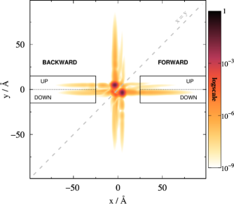
Figure 5: Two-electron density, $\int|\Psi(x,y,R,t=3\text{\,fs})|^{2}\,\mathrm{d}R$, of the fully antisymmetric system (mirror symmetry w.r.t. the $x=y$ diagonal) 3 fs after ionization with an 140 as XUV pulse centered at $T=0$ fs. Four different ionization channels can be distinguished, here illustrated for the emission of the $x$-electron ($x$ direction): Emission occurs either in forward ($x>+25$ Å) or backward ($x<-25$ Å) direction for positive (up) or negative (down) positions of the remaining $y$ electron. The corresponding channels along the $y$-axis are equivalent.

Naturally, the electron densities are symmetric with respect to the $x\!=\!y$-diagonal. It is therefore sufficient to restrict the analysis to electron densities emitted along one axis. Here we chose the $x$ axis and ascribe the labels forward/backward for positive/negative values in $x$. An apparent feature of the single ionization channels is the occurrence of two ionization pathways in every direction. This indicates that the remaining electron eventually stays at different potential minima (around $R=0$), for which we introduce the labels up/down for positive/negative values in $y$, respectively, as indicated in Fig. 5. The electron densities in these four distinct ionization channels differ from each other in shape and amplitude. To distinguish the underlying processes, an evaluation region is defined according to Eqs. (12) and (13) and further separated into subregions $S$ according to the ascribed labels, allowing us to collect and analyze the emitted wave function $\psi^{S}_{\text{out}}(x,y,R,t)$ of each channel separately. As the region of ionization is defined for $\absolutevalue{x}\geq 25$ Å, no emission signal is detected until $t\approx 1$ fs, when the fastest components of the ionized wave function enter the evaluation region. Ionization signal, i.e. $I_{S}(t)=\iiint\absolutevalue{\psi_{\text{out}}^{S}(x,y,R,t)}^{2}\,\mathrm{d}x\,\mathrm{d}y\,\mathrm{d}R$, builds up within a subregion $S$ mainly over the period of $\sim$5 fs. The build up is traced back to a kinetic energy distribution whose central 80% lie between 0.3 and 4.5 eV with a maximum at 1.4 eV. After 5 fs the overall probability to find both electrons in each subregion continues to increase only slightly due to parts of the wave packet with lower kinetic energy entering the subregion. The respective probabilities at 5 fs are $3.9\times 10^{-6}$, $1.1\times 10^{-4}$, $1.8\times 10^{-5}$, and $2.8\times 10^{-5}$ for the forward-up, forward-down, backward-up, and backward-down subregion, respectively.

Fig. 6 shows the time evolution of the average momentum, $\langle p_{y}\rangle^{S}(t)$, of electron $y$, which remains bound in the molecular ion after electron $x$ has been emitted. The quantity $\langle p_{y}\rangle^{S}(t)$ is calculated via the density distribution for the remaining $y$ electron, $\rho_{S}(p_{y},t)$ by integrating over $\psi^{S}_{\text{out}}$ in each individual channels $S$:

$$\langle p_{y}\rangle^{S}(t)=\frac{\int p_{y}\,\rho_{S}(p_{y},t)~{}\differential p_{y}}{\int\rho_{S}(p_{y},t)~{}\differential p_{y}},$$ (19)

where

$$\rho_{S}(p_{y},t)=\iint\left|\widetilde{\psi}_{\text{out}}^{S}(p_{x},p_{y},P,t)\right|^{2}~{}\differential p_{x}~{}\differential P,\\$$ (20)

Here, $\widetilde{\psi}_{\text{out}}^{S}$ is the Fourier-transformed wave function $\psi^{S}_{\text{out}}$. The average momentum $\langle p_{y}\rangle^{S}(t)$ illustrates that all four regions differ in the dynamics induced in the parent ion.

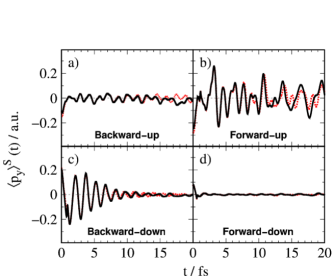
Figure 6: Time-resolved momentum expectation values $\langle p_{y}\rangle^{S}(t)$ of the remaining $y$ electron (black solid lines) after ionization of the full system for the different ionization channels, see Fig. 5, as indicated. For comparison, results from a simulation with a frozen nuclear configuration are added (red dotted lines). The expectation value $\langle p_{y}\rangle^{S}(t)$ of the remaining bound electron $y$ serves as an indicator for electron scattering during the emission process.

In the following, we will interpret the different dynamics seen in Fig. 6a–d based on the leading contributions to photoemission into each evaluation region. However, there are further contributions to each channel, which will be isolated and investigated in Secs. III.2 and III.3.

We interpret the observations as follows: In the forward-down channel, Fig. 6d, the signal stems primarily from the direct emission of the weakly bound electron on the right-hand side of the molecule towards positive $x$ values, i.e. without passing the parent ion (and in particular the other electron) first. The strongly bound electron therefore remains on the left-hand side and is hardly affected by the ionization dynamics which is reflected in the nearly constant momentum expectation value of the remaining electron. In contrast, the oscillating signal in the forward-up channel, Fig. 6b, can be primarily traced back to the strongly bound electron at negative $x$ values being released towards positive $x$ values, such that it first passes the parent ion and the other electron. Its inelastic scattering with the remaining, weakly bound electron induces oscillations of the latter being reflected by the strong time dependence of the remaining electron’s average momentum. We note that the temporal behavior significantly changes for times $t>10$ fs, if the nuclear configuration is frozen during the simulation (red dotted lines) suppressing non-adiabatic transitions.

A similar situation but with reversed roles can be seen for emission into the backward direction: Here, the down channel, Fig. 6c, corresponds to emission of the weakly bound electron after passing the strongly bound one. Thereby, inelastic scattering leads to a regular oscillation in the residual electron’s average momentum $\langle p_{y}\rangle(t)$. Fourier analysis of this oscillation occurring between $t=0$ and 10 fs indicates that the corresponding energy of 2.89 eV can be assigned to the energy gap between the electronic ground and first excited state of the one-electron system (2.78 eV at $R_{0}$), see Fig. 2a. Thus, upon ionization, an electronic wave packet in the residual molecular ion is excited oscillating around the left well’s minimum.

The backward-up channel, Fig. 6a, on the other hand, corresponds to the direct emission of the strongly bound electron without passing the parent ion. A weak response towards a negative average momentum of the remaining electron, can be seen, in particular between 17 and 20 fs, despite the absence of an immediate interaction between the escaping and the remaining electron. This feature is not present if the simulation is performed with a frozen nuclear configuration (dotted red lines). It originates in the induced nuclear dynamics leading to non-adiabatic transitions (intramolecular charge transfer), which will be discussed in more detail in Sec. III.3.

III.2 Reduced wave function: Distinguishable electrons

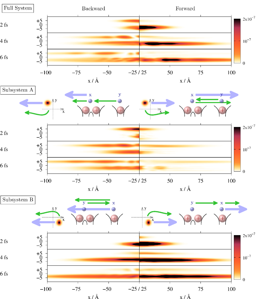
Figure 7: Snapshots of the integrated 2D electronic density $\int|\Psi(x,y,R,t)|^{2}\,\mathrm{d}R$ at $t=$ 2, 4, and 6 fs after ionization of the full system (top panel) and the two subsystems, $\psi_{A}$ (middle panel) and $\psi_{B}$ (bottom panel), with headers illustrating the ionization process (2D view of initial density distribution in the configuration space and 1D view in the real coordinate space). Top: Ionization dynamics of the full system. Middle: Subsystem A with its initial wave packet centered at negative $x$ and positive $y$ values. The up pathways primarily contribute to the total ionization signals (blue arrows) as opposed to the down pathways (green arrows). The initially strongly bound $x$-electron (negative $x$-values) is emitted and the initially weakly bound $y$-electron (positive $y$-values) stays. Bottom: Subsystem B with its initial wave packet centered at positive $x$ and negative $y$ values: Here, the down pathways primarily contribute to the total ionization signals. The initially weakly bound $x$-electron (positive $x$-values) is emitted while the initially strongly bound $y$-electron (negative $y$-values) stays. Oversaturation in the colorbars’ range is used to highlight substructures in the probability density as well as small contributions in the non-dominating pathways. The largest occurring values of the electronic density in forward direction are: (A) $8.3\times 10^{-8}$, (B) $1.3\times 10^{-6}$; and in backward direction: (A) $2.4\times 10^{-7}$, (B) $4.0\times 10^{-7}$.

The previous analysis provided a first intuitive picture of intramolecular scattering effects in the course of ionization. However, as electrons are indistinguishable, the roles of emitted and remaining electrons during the scattering process cannot clearly be identified. To this end, the artificially truncated wave functions $\psi_{A}$ and $\psi_{B}$, see Eqs. (10a) and (10b), are employed as initial conditions, thus rendering the two electrons distinguishable, see Sec. II.2.2. This way, electron-electron correlation originating from the antisymmetry of the wave function and interference effects between the two distinct initial density distributions (localized near $x=\pm 5$ Å & $y=\mp 5$ Å) are neglected. However, a comparison of the probabilities to find the particles in the evaluation regions, $I_{S}(t)$, between the full system and the sum of the subsystems A and B shows very good agreement, indicating that for the present system these types of correlation effects are of minor importance.

In Fig. 7 the time-dependent two-electron densities of the full system with two indistinguishable electrons (upper part) and the subsystems, A (middle part) and B (lower part) with distinguishable electrons, are shown for an area corresponding to the emission of electron $x$ in backward (left panels) and forward direction (right panels), while electron $y$ remains bound to the parent ion. Above the two lower panels, a schematic picture indicates different underlying processes (blue/green arrows) in the $x,y$-configuration space (left) and the one-dimensional coordinate space (right). The thick blue arrows correspond to the four main contributions, i.e. photoemission with and without intramolecular electron-electron scattering, discussed in Sec. III.1, where either the strongly (A) or the weakly bound electron (B) interacts with the electromagnetic field and is released to either side of the molecule.

The first electron wave packet components enter the evaluation region at $x=\pm 25\,$Å between 1 and 2 fs after the interaction with the ionizing pulse. At this instant, electron density is mostly found in the backward-up channel for subsystem A and in the forward-down channel for subsystem B (blue arrows) corresponding to direct photoemission from the side of the molecule closest to the respective subregion. Additionally, a strong slightly delayed signal can be noted stemming from an emission into the opposite direction (blue arrows, A: forward-up, B: backward-down), corresponding to photoemission channels involving intramolecular electron-electron scattering, i.e. the $x$ electron first passing the $y$ electron before beind finally emitted.

The A/B distinction reveals additional signals with a smaller but still significant probability appearing in the down (A) channels and – to an even smaller extent – in the up (B) channels, which are not visible in Fig. 5 due to the larger amplitude of the more dominant signals (blue arrows). Their appearance reveals a correlated motion between the two electrons (indicated by green arrows), where the remaining $y$ electron is relocated (intramolecular charge-transfer) either prior to the photoelectron emission of the $x$ electron or afterwards. This question is addressed in the following section, III.3, by further dissecting the ionization pathways through restricting the electrons’ interaction with the electric field.

III.3 Restricted electron-field interactions

To further investigate the intramolecular dynamics during and after the electron emission process, we perform simulations of the subsystems A and B, i.e. using distinguishable electrons, and restrict the interaction of the electromagnetic field to either the $x$ (ejected) or $y$ (remaining) electron by employing the modified Hamiltonian ${\mathcal{H}}^{\prime}(t)$ defined in Eq. (II.2.3). This way, the absorption process of a system with distinguishable electrons is strictly limited to one specific single electron.

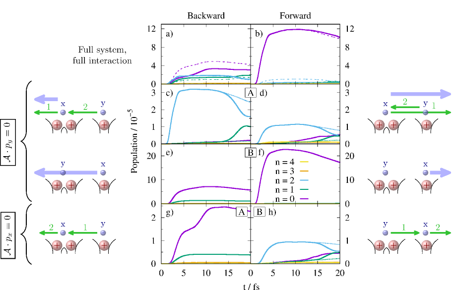
Figure 8: Evolution of the population of the electronic states by the remaining bound $y$-electron calculated via Eq. (21), after the XUV pulse ionizes the two-electron system at $t=0$ fs. The upper panels, (a) and (b), contain the dynamics of the full antisymmetric system, whereas lower panels, (c)–(h), show the dynamics of distinguishable electrons selectively interacting with the electric field as indicated. Dashed lines in panels (a) and (b) correspond to the sum of all individual pathways with restricted field interaction displayed throughout panels (c)–(h). The dotted lines in panels (c), (d), and (h) represent evolution for a molecule with fixed core position. A comprehensive list of all processes can be found in Tab. 1.

The ionization wave function, $\psi^{S}_{\text{out}}(x,y,R,t)$, i.e. the part of the wave function entering the analysis region defined via the mask function, Eq. (13), is projected onto the set of adiabatic eigenfunctions $\{\varphi^{\text{1e}}_{n}(y;R)\},n\in\{0,\dots,4\}$ of the one-electron system, obtained from Eq. (3) and shown in Fig. 2b exemplarily for $R=R_{0}$. Note that these states differ in the electron’s spatial distributions: while for states with the quantum numbers $n\in\{0,1,3\}$, the $y$ electron is located on the (strongly bound) left-hand side, for $n\in\{2,4\}$ electron distribution is predominantly found on the (weakly bound) right-hand side. Thus, a transition between states from different sides corresponds to an intramolecular charge transfer. The population $P^{S^{\prime}}_{n}(t)$ of the $n$th one-electron state by the $y$ electron is calculated as

$$P^{S^{\prime}}_{n}(t)=\iint\left|{\int\varphi^{\text{1e}}_{n}(y;R)\,\psi^{S^{\prime}}_{\text{out}}(x,y,R,t)~{}\mathrm{d}y}\right|^{2}\mathrm{d}x~{}\mathrm{d}R,$$ (21)

where the domain $S^{\prime}$ limits the $x$ integration to either positive or negative values corresponding to the forward ($S^{\prime}=\mathrm{fwd}$) or backward ($S^{\prime}=\mathrm{bwd}$) channel, respectively, but does not distinguish between up- and down-channels anymore. Thus, $P^{S^{\prime}}_{n}(t)$ are the populations of the single-electron states in the evaluation region, i.e. in the molecular parent ion after photoionization. Sketches next to the panels illustrate the dominant ionization pathways with labels ’1’ and ’2’ indicating the temporal order.

The populations are shown in Fig. 8 in backward (left panels, ${x<0}$) and forward direction (right panels, ${x>0}$) for the fully antisymmetric wave function (top panels, a and b) and the subsystems A and B as indicated (lower panels, c–h). The rise in the period of 1 to 5 fs in all panels corresponds to the main part of the wave packet entering the evaluation region. In the subsequent time evolution, the overall probability within the evaluation region remains mostly constant leading to distinct plateau regions in $P^{S^{\prime}}_{n}(t)$. However, small contributions with low kinetic energy (of the emitted $x$ electron) continue to enter the evaluation region at later times, while components with high kinetic energy are removed at the grid boundaries.

Table 1: Various in parts interdependent processes occur during photoionization and contribute to the signal in different evaluation regions for the two subsystems A (with a strongly bound $x$ electron and weakly bound $y$ electron) and B (vice versa). The build up time describes the time frame of the initial wave packet entering the analyzing region (defined by signal above the noise level) until a stable population is reached. $P^{S^{\prime}}_{n}(t)$ in the last column represents the maximum population of this process.

	Channel $S$	$x$	$y$	Process		Fig. 8	build up time / fs	$P^{S^{\prime}}_{\mathrm{n}}$/$10^{-5}$
A	backward-up	$<-25$ Å	$>0$	III	direct emission of the strongly bound electron	c, blue	0.7 - 5.5	$3.1$
	backward-down	$<-25$ Å	$<0$	VI	indirect emission via elastic collision with charge transfer	g, green	1.2 - 14.0	$2.5$
					and subsequent knock up (inelastic scattering)		1.7 - 8.2	$0.4$
				IX	charge transfer via non-adiabatic transition (following III)	c, green	11.2 - 19.0	$1.0$
	forward-up	$>+25$ Å	$>0$	IV	scattered emission of the strongly bound electron	d, blue	1.0 - 5.9	$1.1$
					and subsequent knock up (inelastic scattering)		1.3 - 4.5	$0.1$
	forward-down	$>+25$ Å	$<0$	V	knock down induced charge transfer (following IV)	d, green	6.2 - 16.2	$0.5$
				X	charge transfer via non-adiabatic transition (following IV)	d, green	11.2 - 19.0	$0.5$
B	backward-up	$<-25$ Å	$>0$	Process not visible		—	—	$0.0$
	backward-down	$<-25$ Å	$<0$	II	scattered emission of the weakly bound electron	e, blue	0.8 - 7.2	$6.6$
					and subsequent knock up (inelastic scattering)		1.6 - 7.0	$1.3$
	forward-up	$>+25$ Å	$>0$	VII	indirect emission via elastic collision with charge transfer	h, green	1.5 - 7.1	$0.9$
					and subsequent knock up (inelastic scattering)		2.5 - 4.6	$0.04$
	forward-down	$>+25$ Å	$<0$	I	direct emission of the weakly bound electron	f, blue	0.7 - 5.3	$22.0$
				VIII	knock-down induced charge transfer (following VII)	h, —	4.2 - 18.5	$0.5$
				XI	charge transfer via non-adiabatic transition (following VII)	h, green	9.9 - 19.3	$0.5$

Several processes (indicated by boldface roman numerals) can be identified and separated from each other. They are summarized with their associated ionization channel $S$ in Tab. 1. We first consider the cases, in which the electron (here, the $x$ electron) interacting with the electric field is the one being eventually emitted (Fig. 8c–f). The strongest signal (panel f) corresponds to the emission of the weakly bound electron, initially located near $x=+5$ Å (subsystem B), in forward direction corresponding to a direct photoemission (I) without scattering with the remaining electron. In this case, the strongly bound $y$ electron remains almost unaffected in its position located at the left-hand side (down), corresponding to the electronic ground state of the one-electron system, $n=0$ (see Fig. 2b).

However, the removal of the $x$ electron results in an increase of the $y$ electron’s binding energy corresponding to a shake-down process. The energy change corresponding to a sudden electron removal can be estimated from the potential energy curves at $R_{0}$, $\Delta E_{B}\approx V^{\mathrm{0e}}(R_{0})+V^{\text{2e}}_{0}(R_{0})-V^{\mathrm{1e}}_{0}(R_{0})-V^{\mathrm{1e}}_{2}(R_{0})$ (where $V^{\text{0e}}$ corresponds to the repulsion energy between the movable and the two fixed nuclei only) and accounts for 1.8 eV. Comparing the relative populations at $t=5$ fs, only a very weak shake-up into the one-electron states $n=1$ and 3 is noticed with populations of $P^{\text{fwd}}_{1}/P^{\text{fwd}}_{0}=0.0045$ and $P^{\text{fwd}}_{3}/P^{\text{fwd}}_{0}=0.0004$ relative to the groundstate. This is in line with the almost constant average momentum seen in Fig. 6d for the full (fermionic) system, indicating no coherent dynamics induced.

In contrast, emitting the weaker bound $x$ electron in the opposite (backward) direction, Fig. 8e, such that inelastic scattering with the remaining strongly-bound $y$ electron occurs, entails a significant relative population of the first and third excited one-electron states of $P^{\text{bwd}}_{1}/P^{\text{bwd}}_{0}=0.21$ and $P^{\text{bwd}}_{3}/P^{\text{bwd}}_{0}=0.02$, respectively. Note, that these excited states are still localized on the left-hand side of the molecule (down channel). Since such an excitation does not occur in the forward direction, it must be a result of dynamical correlation between the accelerated $x$ electron and the "inactive" $y$ electron. This interaction corresponds therefore to a pure knock-up process (II) [2]. As a consequence, within 2 and 5 fs, a $y$ electron wave packet can be seen, oscillating within the left potential well, which is reflected in the damped oscillation pattern of the average momentum shown in Fig. 6c.

A similar situation is encountered, when the stronger bound electron (Fig. 8c and d) interacts with the electric field and is ultimately emitted. If the $x$ electron emission occurs in the backward direction, Fig. 8c, again, no intramolecular scattering occurs (III) and the weaker bound $y$ electron remains (initially) in its place, corresponding predominantly to the second excited state, $n=2$, which is localized on the molecule’s right-hand side (up channel). Again, a shake-down stabilization of the binding energy of approximately 1.8 eV is expected and only a very weak shake-up to state $n=4$ is noted ($P^{\text{bwd}}_{4}/P^{\text{bwd}}_{2}=0.0048$).

In the forward direction, i.e. with immediate electron-electron interaction (IV), Fig. 8d, the second excited state is dominant, too but also shows a considerable knock-up process ($P^{\text{fwd}}_{4}/P^{\text{fwd}}_{2}=0.10$). Additionally, an increase in the population of the one-electron ground state, $n=0$, can be noted. Therefore, inelastic intramolecular scattering with the weaker bound $y$ electron must have taken place resulting in a knock-down process (V) of the $y$ electron during the $x$ electron emission from the (stronger bound) lower energy levels. Comparing their respective peaks, the relative population achieved through the knock-down process is $P^{\text{fwd}}_{0}/P^{\text{fwd}}_{2}=0.45$. Since in the energetically lower $n=0$ state, the $y$ electron is located on the left-hand side, this correlation-driven process coincides with an intramolecular charge transfer (green arrows).

Finally, the lowest panels, Fig. 8g and h, correspond purely to correlation-driven processes, in which the energy provided by the electric field is absorbed by electron $y$, but results eventually in the emission of electron $x$. Therefore, a nearly elastic collision between the two electrons must have occurred, in which the absorbing electron ($y$) transfers most of its acquired kinetic energy to the electron originally unaffected by the field ($x$). This "indirect photoemission" process (VI,VII), is very similar to the two-step-one (TS1) process in double ionization, where the electron emitted first pushes another electron out of an atom in a second step after photoabsorption [10]. But in our case, the initially accelerated electron is not released in the end but rather takes the place of the subsequently emitted electron – similar to the elastic collision between billiard balls. Consequently, the resulting populations of the single-electron states of the remaining electron shown in Fig. 8g for subsystem A resemble the one of subsystem B, seen in panel e, where the remaining electron is located at the strongly bound side. The same applies for subsystem B’s elastic collision process, Fig. 8h, which rather resembles the populations found in A’s inelastic scattering, panel d including knock-up (within VII) and knock-down (VIII) features. Again, this is traced back to the accelerated $y$ electron taking $x$’s place prior to the emission of the $x$ electron. Note that the indirect photoemission leads to a charge transfer (through elastic collision) immediately after photoabsorption. We therefore conclude that the significant early signals, seen in Fig. 7 in subsystem A’s backward-down channel (and with a lower amplitude also in subsystem B’s forward-up channel) correspond to the elastic collision process preceding the $x$ electron’s emission.

In panels c,d, and h of Fig. 8, where the $n=2$ state is predominantly occupied, a decrease occurs in $P^{S^{\prime}}_{2}(t)$ after approximately $t\approx 15$ fs with a simultaneous increase of the $n=1$ state, $P^{S^{\prime}}_{1}(t)$. This time-dependent feature can be traced back to the non-adiabatic nuclear reorganization dynamics (IX,X,XI) induced by the ionization process. Note that these transitions do not occur, if the simulation is performed with a frozen nuclear configuration (dotted lines). Fig. 9 shows the correlated electron-nuclear dynamics for subsystem A with emission in backward direction (corresponding to Fig. 8c) through the density function $\int\left|\psi_{\text{out}}^{\text{bwd}}(x,y,R,t)\right|^{2}\,\mathrm{d}x$. It can be seen that during the first 14 fs, the shape of the electronic part only marginally changes, while the center of the nuclear distribution moves from $R_{0}=-2.05$ Å towards larger values. This dynamics is induced by the Coulomb attraction between the remaining electron and the mobile nucleus, but is also consistent with the potential energy surface of the second state, $V^{\text{1e}}_{2}(R)$, see Fig. 2a upper panel. The latter one exhibits a large gradient towards the molecular center ($R=0$), where a coupling region with the first excited state, $V^{\text{1e}}_{1}(R)$, is found. Indeed, at 17 fs, the center of the nuclear distribution passes the origin and the electronic distribution begins to shift towards the left-hand side (to negative $y$ values), which is reflected in a slightly negative instantaneous average electronic momentum $\langle p_{y}\rangle^{\mathrm{backward-up}}(t)$ in the case of direct photoionization in the backward-up channel, cf. Fig. 6a, which is not present in the case of frozen nuclei (red dotted line). Therefore, upon ionization, nuclear dynamics is initiated, driving the system via non-adiabatic transition from the second to the first electronically excited state, $\varphi^{\text{1e}}_{2}(y;R)\rightarrow\varphi^{\text{1e}}_{1}(y;R)$ corresponding to an intramolecular charge transfer. Note, however, that this process is significantly slower than the charge transfer process driven by electronic correlation.

It is noteworthy that, here, despite these non-adiabatic transitions, the nuclear dynamics does not seem to affect the various ionization processes discussed above. We attribute this to the chosen near-equilibrium initial conditions for $\chi(R)$. Previous studies have shown, that nuclear dynamics following initial non-equilibrium configurations is reflected in the photoelectron momentum distribution [37, 38]. Investigations of such effects on the correlation-driven knock-up and knock-down processes are currently under way in our workgroup.

To summarize, all observed processes, i.e. direct photoemission with and without inelastic scattering leading to knock-up and knock-down transitions, as well as indirect photoemission through elastic collision, and non-adiabatic transitions, are summarized in Tab. 1 together with their individual amplitudes at their respective maximum and build up times, i.e. the time span the corresponding wave packet requires to achieve approximately stable populations within the observed time window. These times differ for the individual processes mostly due to the different travelling distances (direct emission vs. scattered and indirect emissions) for the ejected electron to reach the evaluation zone and because of differences in their kinetic energies. However, the slightly longer timescales of knock-down processes in particular indicate a more complex electron-electron dynamics within the molecular system prior to the electron release.

Regarding the relative amplitudes, we note, that the correlation-driven pathways through elastic and inelastic scattering appear to be nearly of the same order of magnitude as the direct photoemission. This can be seen in Fig. 8a and b, where the dynamics of the fully antisymmetric initial wave function without any restrictions on the electric-field interaction (solid lines) is qualitatively reproduced by the artificially restricted subsystems (dashed lines, corresponding to the direct sum of all individual pathways with restricted field interaction). Remaining discrepancies stem most likely from the missing simultaneous interaction of the XUV pulse with both electrons and also from the omission of interference effects between emitted density from the two initial localized electronic density distributions, which we have dropped by regarding electrons as distinguishable particles.

We conclude that the final state of the molecular parent ion after ionization depends strongly on dynamical correlation between electrons through elastic and inelastic intramolecular scattering events preceding the electron emission beyond static shake-up effects. Furthermore, we showed that such effects also significantly contribute to the total ionization probability. In particular, quantifying the effect of correlation-driven knock-up/knock-down processes and the indirect photoemission processes on the same magnitude as direct photoionization processes, underlines the deficiencies of the commonly applied single active electron approximation as well as the sudden approximation – even in the context of single-photon ionization of molecules.

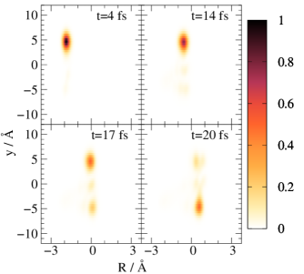
Figure 9: Electron-nuclear density of subsystem A in the backward channel, $\int\left|\psi_{\mathrm{out}}^{\mathrm{bwd}}(x,y,R)\right|^{2}\,\mathrm{d}x$. Here, the strongly bound $x$ electron is emitted and the $y$ electron remains initially on weakly bound side ($y>0$), before non-adiabatic transitions around $R=0$ lead to a charge transfer with significant electron density at the molecule’s left-hand side ($y<0$).

IV Summary

We investigated the correlated electron-electron and electron-nuclear dynamics in a one-dimensional molecular charge-transfer model by solving the time-dependent Schrödinger equation numerically for two electronic and one nuclear degree of freedom. To this end, we considered ionization of a single electron by an ultrashort XUV pulse and investigated the exact scattering mechanism by carefully backtracking the electron’s interaction with the residual cation and in particular with the remaining bound electron.

We introduced different theoretical approaches to investigate the correlated electron dynamics and nuclear motion during and after the pulse interaction. First, by removing all unionized components from the total wave function and projection on the one-electron system to quantify shake and knock processes. Second, we dissected these processes and identified different contributions of ionization pathways by replacing the fermionic wave functions by that of two "distinguishable" electrons and by restricting the interaction of the XUV pulse to a specific electron within the molecule. Using this approach, time-dependent signatures in the evolution of the molecular parent ion were identified and traced back to various intramolecular scattering events on different time scales.

Thereby, we went beyond commonly employed approximations such as the sudden approximation, frozen nuclear degrees of freedom, or the single active electron approximation. Thus, significant contributions from electron-electron and non-adiabatic interactions within the single-photon ionization process were revealed on the atto- and femtosecond timescale. In particular, relevant pathways to the overall signal were isolated, in which inelastic scattering resulted in knock-up and knock-down phenomena beyond the typically regarded (sudden) shake effects. Additional pathways of significant contribution involving elastic scattering were found, where the electron originally accelerated by the electric field transfers its momentum to a different electron within the molecule and takes its place instead (indirect photoemission). Our analysis revealed differences in the temporal signatures of all identified processes and allowed to estimate their relevance within the overall photoemission process. It was shown that electron-correlation driven processes occur on the same order of magnitude as the direct photoemission. While for a two-electron system the amplitude of the elastic collision process may be overestimated due to the reduced dimensionality of the model system, we expect this process to become even more relevant in larger, multi-electron systems. Furthermore, it was shown that different ionization pathways leave the parent molecular ion in different electronic states. As a consequence, correlated electron-nuclear reorganization dynamics is induced.

We believe that the observations made here for a model system are representative for molecular systems and consequently that both, elastic and inelastic scattering among electrons, contribute significantly to the ionization processes and the postionization dynamics through various pathways beyond the single active electron picture.