ARMA Nets:
Expanding Receptive Field for Dense Prediction

Abstract

Global information is essential for dense prediction problems, whose goal is to compute a discrete or continuous label for each pixel in the images. Traditional convolutional layers in neural networks, initially designed for image classification, are restrictive in these problems since the filter size limits their receptive fields. In this work, we propose to replace any traditional convolutional layer with an autoregressive moving-average (ARMA) layer, a novel module with an adjustable receptive field controlled by the learnable autoregressive coefficients. Compared with traditional convolutional layers, our ARMA layer enables explicit interconnections of the output neurons, and learns its receptive field by adapting the autoregressive coefficients of the interconnections. ARMA layer is adjustable to different types of tasks: for tasks where global information is crucial, it is capable of learning relatively large autoregressive coefficients to allow for an output neuron’s receptive field covering the entire input; for tasks where only local information is required, It can learn small or near zero autoregressive coefficients and automatically reduces to a traditional convolutional layer. We show both theoretically and empirically that the effective receptive field of networks with ARMA layers (named as ARMA networks) expands with larger autoregressive coefficients. We also provably solve the instability problem of learning and prediction in the ARMA layer through a re-parameterization mechanism. Additionally, we demonstrate that ARMA networks substantially improve their baselines on challenging dense prediction tasks including video prediction and semantic segmentation.

1 Introduction

Convolutional layers in neural networks have many successful applications for machine learning tasks. Each output neuron encodes an input region of the network measured by the effective receptive field (ERF) [24]. A large ERF that allows for sufficient global information is needed to make accurate predictions; however, a simple stack of convolutional layers does not effectively expand ERF. Convolutional neural networks (CNNs) typically encode global information by adding downsampling (pooling) layers, which coarsely aggregate global information. A fully-connected classification layer subsequently reduces the entire feature map to an output label. Downsampling and fully-connected layers are suitable for image classification tasks where only a single prediction is needed. But they are less effective, due to potential loss of information, in dense prediction tasks such as semantic segmentation and video prediction, where each pixel requests a prediction. Therefore, it is crucial to introduce mechanisms that enlarge ERF without too much information loss.

Naive approaches to expanding ERF, such as deepening the network or enlarging the filter size, drastically increase the model complexity, which results in expensive computation, difficulty in optimization, and susceptibility to overfitting. Recently advanced architectures have been proposed to expand ERF, including encoder-decoder structured networks [29], dilated convolutional networks [39, 40], and non-local attention networks [33]. However, encoder-decoder structured networks could lose high-frequency information due to the downsampling layers. Dilated convolutional networks could suffer from the gridding effect while the ERF expansion is limited, and non-local attention networks are expensive in training and inference.

We introduce a novel autoregressive-moving-average (ARMA) layer that enables adaptive receptive field by explicit interconnections among its output neurons. Our ARMA layer realizes these interconnections via extra convolutions on output neurons, on top of the convolutions on input neurons as in a traditional convolutional layer. We provably show that an ARMA network can have arbitrarily large ERF, thus encoding global information, with minimal extra parameters at each layer. Consequently, an ARMA network can flexibly enlarge its ERF to leverage global knowledge for dense prediction without reducing spatial resolution. Moreover, the ARMA networks are independent of the architectures above including encoder-decoder structured networks, dilated convolutional networks and non-local attention networks.

A significant challenge in ARMA networks lies in the complex computations needed in both forward and backward propagations — simple convolution operations are not applicable since the output neurons are influenced by their neighbors and thus interrelated. Another challenge in ARMA networks is instability — the additional interconnections among the output neurons could recursively amplify the outputs and lead them to infinity. We address both challenges in this paper.

Summary of Contributions

• We introduce a novel ARMA layer that is a plug-and-play module substituting convolution layers in neural networks to allow flexible tuning of their ERF, adapting to the task requirements and improving performance in dense prediction problems.

• We recognize and address the problems of computation and instability in ARMA layers. (1) To reduce computational complexity, we develop FFT-based algorithms for both forward and backward passes; (2) To guarantee stable learning and prediction, we propose a separable ARMA layer and a re-parameterization mechanism that ensures the layer to operate in a stable region.

• We successfully apply ARMA layers in ConvLSTM network [38] for pixel-level multi-frame video prediction and U-Net model [29] for medical image segmentation. ARMA networks substantially outperform the corresponding baselines on both tasks, suggesting that our proposed ARMA layer is a general and useful building block for dense prediction problems.

2 Related Works

Dilated convolution [14] enlarges the receptive field by upsampling the filter coefficients with zeros. Unlike encoder-decoder structure, dilated convolution preserves the spatial resolution and is thus widely used in dense prediction problems, including semantic segmentation [23, 39, 6], and objection detection [9, 19]. However, dilated convolution by itself creates gridding artifacts if its input contains higher frequency than the upsampling rate [40], and the inconsistency of local information hampers the performance of the dilated convolutional networks [34]. Such artifacts can be alleviated by extra anti-aliasing layer [40], group interacting layer [34] or spatial pyramid pooling [7].

Deformable convolution allows the filter shape (i.e. locations of the incoming pixels) to be learnable [10, 15, 41]. While deformable convolution focuses on adjusting the filter shape, our ARMA layer aims to expand the filter size adaptively.

Non-local attention network [33] inserts non-local attention blocks between the convolutional layers. A non-local attention block computes a weighted sum of all input neurons for each output neuron, similar to attention mechanism [32]. In practice, non-local attention blocks are computationally expensive, thus they are typically inserted in the upper part of the network (with lower resolution). In contrast, our ARMA layers are economical (see section 4), and can be used throughout the network.

Encoder-decoder structured network pairs each downsampling layer with another upsampling layer to maintain the resolution, and introduces skip-connection between the pair to preserve the high-frequency information [29, 23]. Since the shortcut bypasses the downsampling/upsampling layers, the network has a small receptive field for the high-frequency components. A potential solution is to augment upsampling with non-local attention block [26] or ARMA layer (section 6).

Spatial recurrent neural networks apply recurrent propagations over the spatial domain  [4, 27, 16, 31, 22], and learns the affinity between neighboring pixels [21]. Most of these prior works consider nonlinear recurrent neural networks, where the activation between recursions prohibits an efficient FFT-based algorithm. In contrast, our proposed ARMA layer is equivalent to a linear recurrent neural network. where the spatial recurrences in ARMA layer can be efficiently evaluated using FFT.

3 ARMA Neural Networks

In this section, we introduce a novel autoregressive-moving-average (ARMA) layer, and analyze its ability to expand Effective Receptive Field (ERF) in neural networks. The analysis is further verified by visualizing the ERF with varying network depth and strength of autoregressive coefficients.

3.1 ARMA Layer

A traditional convolutional layer is essentially a moving-average model [3], $\mathcal{Y}_{\bm{:},\bm{:},t}=\sum_{s=1}^{S}\mathcal{W}_{\bm{:},\bm{:},t,s}\ast\mathcal{X}_{\bm{:},\bm{:},s}$, where the moving-average coefficients $\mathcal{W}\in\mathbb{R}^{K_{m}\times K_{m}\times T\times S}$ is parameterized by a $4^{\text{th}}$-order kernel ($K_{m}$ is the filter size, and $S,T$ are input/output channels), $\bm{:}$ denotes all elements from the specified coordinate, and $\ast$ denotes convolution between an input feature and a filter.

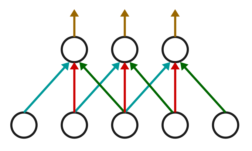
(a) Convolution

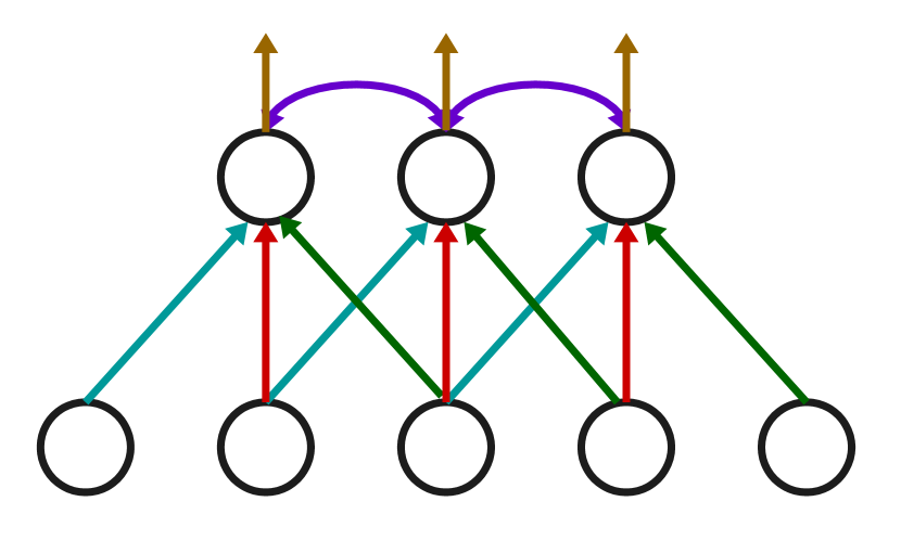
(b) ARMA

Figure 1: The ARMA layer introduces interconnections among output neurons explicitly.

As motivated in the introduction, we introduce a novel ARMA layer, that enables adaptive receptive field by introducing explicit interconnections among its output neurons as illustrated in Figure 1. Our ARMA layer realizes these interconnections by introducing extra convolutions on the outputs, in addition to the convolutions on the inputs as in a traditional convolutional layer. As a result, in an ARMA layer, each output neuron can be affected by an input pixel faraway through interconnections among the output neurons, thus receives global information. Formally, we define ARMA layer in Definition 1.

Definition 1 (ARMA layer).

An ARMA layer is parameterized by a moving-average kernel (coefficients) $\mathcal{W}\in\mathbb{R}^{K_{m}\times K_{m}\times S\times T}$ and an autoregressive kernel (coefficients) $\mathcal{A}\in\mathbb{R}^{K_{a}\times K_{a}\times T}$. It receives an input $\mathcal{X}\in\mathbb{R}^{I_{1}\times I_{2}\times S}$ and returns an output $\mathcal{Y}\in\mathbb{R}^{I^{\prime}_{1}\times I^{\prime}_{2}\times T}$ with an ARMA model:

$$\mathcal{A}_{\bm{:},\bm{:},t}\ast\mathcal{Y}_{\bm{:},\bm{:},t}=\sum_{s=1}^{S}\mathcal{W}_{\bm{:},\bm{:},t,s}\ast\mathcal{X}_{\bm{:},\bm{:},s}$$ (1)

Remarks: (1) Since the output interconnections are realized by convolutions, the ARMA layer maintains the shift-invariant property. (2) The ARMA layer reduces to a traditional layer if the autoregressive kernel $\mathcal{A}$ represents an identical mapping. (3) The ARMA layer is a plug-and-play module that can replace any convolutional layer, adding $K_{a}^{2}T$ extra parameters negligible compared to $K_{w}^{2}ST$ parameters in a traditional convolution layer. (4) Different from traditional layer, computing Equation 1 and its backpropagation is nontrivial, studied in section 4.

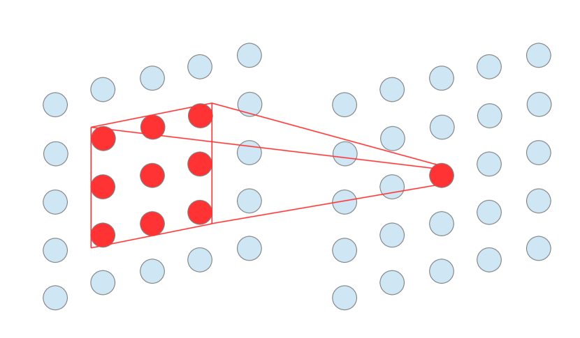
(a) Convolution

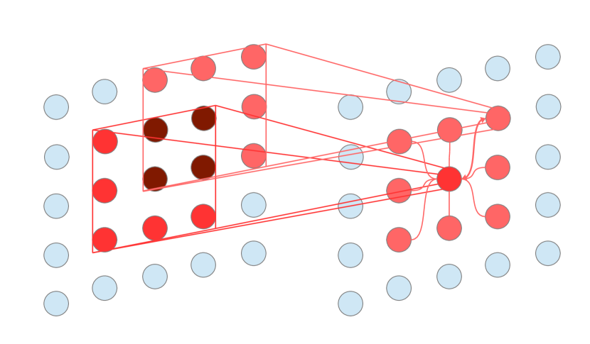
(b) ARMA

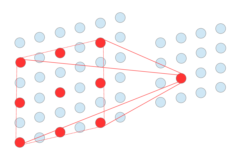
(c) Dilated convolution

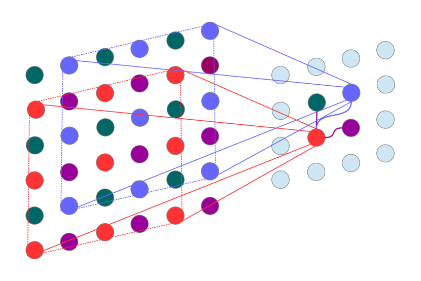
(d) Dilated ARMA

Figure 2: Diagrams of receptive field. In ARMA layer (b), each output neuron receives its neighbors’ receptive field. In (d), ARMA’s autoregression fills the gaps created by dilated convolution.

Our ARMA layer is complementary to dilated convolutional layer, deformable convolutional layer, non-local attention block and encoder-decoder architecture, and can be combined with each of them. For instance, dilated ARMA layer, illustrated in 2(d), removes the gridding effect caused by dilated convolution — the autoregressive kernel can be interpreted as an anti-aliasing filter.

The motivation of introducing ARMA layer is to enlarge the effective input region for each network output without increasing the filter size or network depth, thus avoiding the difficulties in training larger or deeper models. As illustrated in Figure 2, each output neuron in a traditional convolutional layer (2(a)) only receives information from a small input region (the filter size). However, an ARMA layer enlarges the region from a local small one to a larger one (2(b)), and enables an output neuron to receive information from a faraway input neuron through the connections to its neighbors. Now we formally introduce the concept of effective receptive field (ERF) to characterize the effective input region. And we will provably show that an ARMA network can have arbitrarily large ERF with a single extra parameter at each layer in Theorem 3 in the following subsection.

3.2 Effective Receptive Field

Effective receptive field (ERF) [24] measures the area of the input region that makes substantial contribution to an output neuron. In this section, we analyze the ERF size of an $L$-layers network with ARMA layers v.s. traditional convolutional layers. Formally, consider an output at location $(i_{1},i_{2})$, the impact from an input pixel at $(i_{1}-p_{1},i_{2}-p_{2})$ (i.e   $L$ layers and $(p_{1},p_{2})$ pixels away) is measured by the amplitude of partial derivative $g(i_{1},i_{2},p_{1},p_{2})=\left|{\partial{\mathcal{Y}^{(L)}_{i_{1},i_{2},t}}}/{\partial{\mathcal{X}^{(1)}_{i_{1}-p_{1},i_{2}-p_{2},s}}}\right|$ (where superscripts index the layers), i.e. how much the output changes as the input pixel is perturbed.

Definition 2 (Effective Receptive Field, ERF).

Consider an $L$-layers network with an $S$-channels input $\mathcal{X}^{(1)}\in\mathbb{R}^{I_{1}\times I_{2}\times S}$ and a $T$-channels output $\mathcal{Y}^{(L)}\in\mathbb{R}^{I_{1}\times I_{2}\times T}$, its effective receptive field is defined as the empirical distribution of the gradient maps: $\text{ERF}(p_{1},p_{2})={1/(I_{1}I_{2}ST)}\cdot\sum_{s,t,i_{1},i_{2}}\allowbreak[{g(i_{1},i_{2},p_{1},p_{2})}\allowbreak/{\sum_{j_{1},j_{2}}g(j_{1},j_{2},p_{1},p_{2})}]$, To measure the size of the ERF, we define its radius $r(\textsl{ERF})$ as the standard deviation of the empirical distribution:

$$r^{2}\left(\textsl{ERF}\right)=\sum_{p_{1},p_{2}}\left(p_{1}^{2}+p_{2}^{2}\right)\textsl{ERF}\left(p_{1},p_{2}\right)-\left[\sum_{p_{1},p_{2}}\sqrt{p_{1}^{2}+p_{2}^{2}}\leavevmode\nobreak\ \textsl{ERF}(p_{1},p_{2})\right]^{2}$$ (2)

Notice that ERF simultaneously depends on the model parameters and a specified input to the network, i.e. ERF is both model-dependent and data-dependent. Therefore, it is generally intractable to compute the ERF analytically for any practical neural network.

We follow the original paper of ERF [24] to estimate the radius with a simplified linear network. The paper empirically verifies that such an estimation is accurate and can be used to guide filter designs.

Theorem 3 (ERF of a linear ARMA network with dilated convolutions).

Consider an $L$-layers linear network, where the $\ell^{\text{th}}$ layer computes $y^{(\ell)}_{i}-{a}^{(\ell)}y^{(\ell)}_{i-1}=\sum_{p=0}^{{K}^{(\ell)}-1}[(1-{a}^{(\ell)})/{K}^{(\ell)}]\cdot y^{(\ell-1)}_{i-{d}^{(\ell)}p}$ (i.e. the moving-average coefficients are uniform with length ${K}^{(\ell)}$ and dilation ${d}^{(\ell)}$, and the autoregressive coefficients $a^{(\ell)}_{0}=1,a^{(\ell)}_{1}=-{a}^{(\ell)}$ has length $2$). Suppose $0\leq{a}^{(\ell)}<1$ for $1\leq\ell\leq L$, the ERF radius of such a linear ARMA network is

$$r(\text{ERF})_{\text{ARMA}}^{2}=\sum_{\ell=1}^{L}\left[\frac{{{d}^{(\ell)}}^{2}\left({{K}^{(\ell)}}^{2}-1\right)}{12}+\frac{{a}^{(\ell)}}{\left(1-{a}^{(\ell)}\right)^{2}}\right]$$ (3)

When ${a}^{(\ell)}=0,\forall\ell\in[L]$, the ARMA layers reduce to (dilated) convolutional layers, and the ERF of the resulted linear CNN has radius $r(\text{ERF})_{\text{CNN}}^{2}=\sum_{\ell=1}^{L}{{d}^{(\ell)}}^{2}({{K}^{(\ell)}}^{2}-1)/12$.

Theorem 3 is proved in Appendix B. If the coefficients for different layers are identical, the radius reduces to $r(\text{ERF})_{\text{ARMA}}=\sqrt{L}\cdot\sqrt{d^{2}(K^{2}-1)/12+a/(1-a)^{2}}$.

Remarks: (1) Compared with a (dilated) CNN, an ARMA network can have arbitrarily large ERF with an extra parameter $a$ at each layer. When the autoregressive coefficient $a$ is large (e.g. $a>1-1/(dK)$), the second term $a/(1-a)^{2}$ dominates the radius, and the ERF is substantially larger than that of a CNN. In particular, the radius tends to infinity as $a$ approaches $1$. (2) An ARMA network can adaptively adjust its ERF through learnable parameter $a$. As $a$ gets smaller (e.g. $a<1-1/(dK)$), the second term is comparable to or smaller than the first term, and the effect of expanded ERF diminishes. In particular if $a=0$, an ARMA network reduces to a CNN.

Visualization of the ERF. In Theorem 3, we analytically show that the ARMA’s radius of ERF increases with the network depth and magnitude of the autoregressive coefficients. We now verify our analysis by simulating linear ARMA networks with a single extra parameter (an autoregressive coefficient $a$) in each layer under varying depths and magnitude of the autoregressive coefficient $a$. Shown in Figure 3, as the autoregressive coefficient get larger, the radius of the ERF increases. When the autoregressive coefficient is zero (i.e. $a=0$), an ARMA network reduces to a traditional convolutional network. The simulation results also indicate that the ERF expands as the networks get deeper, and ARMA’s ability to expand the ERF increases as the networks get deeper. In conclusion, an ARMA network can have a large ERF even when the network is shallow, and its ability to expand the ERF increases as the network gets deeper.

a	$L=1$ $L=3$ $L=5$	a	$L=1$ $L=3$ $L=5$
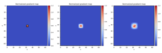
$0.0$ (CNN)		$0.8$
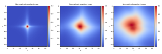
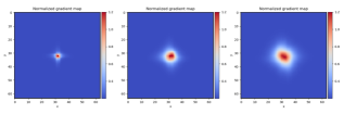
$0.6$		$0.9$

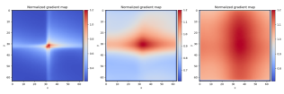
Figure 3: Visualization of ERF in linear ARMA networks with a single extra parameter (an autoregressive coefficient $a$) in each layer, under different network depth $L=1,3,5$ and different magnitude of the autoregressive coefficient $a=0.0,0.6,0.8,0.9$.

4 Prediction and Learning of ARMA Layer

In the ARMA layer, each neuron is influenced by its neighbors from all directions (see 2(b)). As a result, no neurons could be evaluated alone before evaluating any other neighboring neurons. To compute Equation 1, we thus need to solve a system of linear equations to obtain all values simultaneously. (1) However, the standard solver using Gaussian elimination is too expensive to be practical, and therefore we need to seek for a more efficient solution. (2) Furthermore, the solver for the system of linear equations is typically not automatic differentiable, and we have to derive the backward equations analytically. (3) Finally, we also need to devise an efficient algorithm to compute the backpropagation equations efficiently. In the section, we address these aforementioned problems.

Decomposing ARMA Layer. We decompose the ARMA layer in Equation 1 into a moving-average (MA) layer and an Autoregressive layer, with $\mathcal{T}\in\mathbb{R}^{I_{1}\times I_{2}\times T}$ as an intermediate result:

$$\textsf{MA Layer: }\leavevmode\nobreak\ \mathcal{T}_{\bm{:},\bm{:},t}=\sum_{s=1}^{S}\mathcal{W}_{\bm{:},\bm{:},t,s}\ast\mathcal{X}_{\bm{:},\bm{:},s};\quad\textsf{AR Layer: }\leavevmode\nobreak\ \mathcal{A}_{\bm{:},\bm{:},t}\ast\mathcal{Y}_{\bm{:},\bm{:},t}=\mathcal{T}_{\bm{:},\bm{:},t}$$ (4)

Layer	# params.	# FLOPs	$r(\textsl{ERF})^{2}$
Conv.	$K_{w}^{2}C^{2}$	$O(I^{2}K_{w}^{2}C^{2})$	$O(LK_{w}^{2})$
ARMA	$\begin{gathered}K_{w}^{2}C^{2}\\ +{\color[rgb]{1,0,0}K_{a}^{2}C}\end{gathered}$	$\begin{gathered}O(K_{w}^{2}I^{2}C^{2}+\\ {\color[rgb]{1,0,0}I^{2}\log(I)\ C})\end{gathered}$	$\begin{gathered}O\big{(}LK_{w}^{2}+\\ {\color[rgb]{0,0,1}L\frac{a}{(1-a)^{2}}}\big{)}\end{gathered}$

Table 1: ARMA layer achieves large gain of ERF radius through small overhead of extra # of parameters and # of FLOPs. Through a single extra parameter $a$ (thus $K_{a}=2$), the ERF radius can be arbitrarily large. For notational simplicity, we assume the heights/widths are equal $I_{1}$$=$$I_{2}$$=$$I_{1}^{\prime}$$=$$I_{2}^{\prime}$$=$$I$, and the input and output channels are the same $S$$=$$T$$=$$C$.

Difficulty in Computing the AR Layer. While the MA layer is simply a traditional convolutional layer, it is nontrivial to solve the AR layer. Naively using Gaussian elimination, the linear equations in the AR layer can be solved in time cubic in dimension $O((I_{1}^{2}+I_{2}^{2})I_{1}I_{2}T)$, which is too expensive.

Solving the AR Layer. We propose to use the frequency-domain division [20] to solve the deconvolution problem in the AR layer. Since the convolution in spatial domain leads to element-wise product in frequency domain, we first transform $\mathcal{A},\mathcal{T}$ into their frequency representations $\mathcal{\widetilde{A}},\mathcal{\widetilde{T}}$, with which we compute $\mathcal{\widetilde{Y}}$ (the frequency representation of $\mathcal{Y}$) with element-wise division. Then, we reconstruct the output $\mathcal{Y}$ by an inverse Fourier transform of $\mathcal{\widetilde{Y}}$.

Computational Overhead. ARMA trades small overhead of extra number of parameters and computation for large gain of ERF radius as shown in Table 1. With Fast Fourier Transform (FFT), the FLOPS required by the extra autoregressive layer is $O(\log(\max(I_{1},I_{2}))I_{1}I_{2}T)$ (see Appendix C for derivations). Importantly, compared with non-local attention block [33], the extra computation introduced in a ARMA layer is smaller; a non-local attention block requires $O(I_{1}^{2}I_{2}^{2}T)$ FLOPS.

Backpropagation. Deriving the backpropagation for Equation 4 is nontrivial; although backpropagation rule for MA layer is conventional, that of AR layer is not. In Theorem 4 we show that backpropagation of an AR layer can be computed as two ARMA models.

Theorem 4 (Backpropagation of ARMA layer).

Given $\mathcal{A}_{\bm{:},\bm{:},t}\ast\mathcal{Y}_{\bm{:},\bm{:},t}=\mathcal{T}_{\bm{:},\bm{:},t}$ and the gradient ${\partial\mathcal{L}}/{\partial{\mathcal{Y}}}$, the gradients $\{{\partial\mathcal{L}}/{\partial{\mathcal{A}}},{\partial\mathcal{L}}/{\partial{\mathcal{X}}}\}$ can be obtained by two ARMA models:

$$\mathcal{A^{\top}}_{\bm{:},\bm{:},t}\ast\frac{\partial\mathcal{L}}{\partial{\mathcal{A}_{\bm{:},\bm{:},t}}}=-\mathcal{Y^{\top}}_{\bm{:},\bm{:},t}\ast\frac{\partial\mathcal{L}}{\partial{\mathcal{Y}_{\bm{:},\bm{:},t}}};\quad\mathcal{A^{\top}}_{\bm{:},\bm{:},t}\ast\frac{\partial\mathcal{L}}{\partial{\mathcal{T}_{\bm{:},\bm{:},t}}}=\frac{\partial\mathcal{L}}{\partial{\mathcal{Y}_{\bm{:},\bm{:},t}}}$$ (5)

where $\mathcal{A^{\top}}_{\bm{:},\bm{:},t}$ and $\mathcal{Y^{\top}}_{\bm{:},\bm{:},t}$ are the transposed images of $\mathcal{A}_{\bm{:},\bm{:},t}$ and $\mathcal{Y}_{\bm{:},\bm{:},t}$ (e.g. $\mathcal{A^{\top}}_{i_{1},i_{2},t}=\mathcal{A}_{-i_{1},-i_{2},t}$).

Since the backpropagation is characterized by ARMA models, it can be evaluated efficiently using FFT similar to Equation 4. The proof of Theorem 4 with its FFT evaluation is given in Appendix C.

5 Stability of ARMA Layers

An ARMA model with arbitrary coefficients is not always stable. For example, the model $y_{i}-ay_{i-1}=x_{i}$ is unstable if $|a|>1$: Consider an input $\bm{x}$ with $x_{0}=1$ and $x_{i}=0,\forall i\neq 0$, the output $\bm{y}$ will recursively amplify itself as $y_{0}=1,y_{1}=a,\cdots,y_{i}=a^{i}$ and diverge to infinity.

5.1 Stability Constraints for ARMA layer

The key to guarantee stability of an ARMA layer is to constrain its autoregressive coefficients, which prevents the output from repeatedly amplifying itself. To derive the constraints, we propose a special design, separable ARMA layer inspired by separable filters [20].

Definition 5 (Separable ARMA Layer).

A separable ARMA layer is parameterized by a moving-average kernel $\mathcal{W}\in\mathbb{R}^{K_{w}\times K_{w}\times S\times T}$ and $T\times Q$ sets of autoregressive filters $\{(f^{(q)}_{\bm{:},t},g^{(q)}_{\bm{:},t})_{q=1}^{Q}\}_{t=1}^{T}$,. It takes an input $\mathcal{X}\in\mathbb{R}^{I_{1}\times I_{2}\times S}$ and returns an output $\mathcal{Y}\in\mathbb{R}^{I^{\prime}_{1}\times I^{\prime}_{2}\times T}$ as

$$\left(f^{(1)}_{\bm{:},t}\ast\cdots\ast f^{(Q)}_{\bm{:},t}\right)\otimes\left(g^{(1)}_{\bm{:},t}\ast\cdots\ast g^{(Q)}_{\bm{:},t}\right)\ast\mathcal{Y}_{\bm{:},\bm{:},t}=\sum_{s=1}^{S}\ \mathcal{W}_{\bm{:},\bm{:},t,s}\ast\mathcal{X}_{\bm{:},\bm{:},s}$$ (6)

where the filters $f^{(q)}_{\bm{:},t},g^{(q)}_{\bm{:},t}\in\mathbb{R}^{3}$ are length-$3$, and $\otimes$ denotes outer product of two 1D-filters.

Remarks: Each autoregressive filter $\mathcal{A}_{\bm{:},\bm{:},t}$ is designed to be separable, i.e. $\mathcal{A}_{\bm{:},\bm{:},t}=F_{\bm{:},t}\otimes G_{\bm{:},t}$, thus it can be characterized by 1D-filters $F_{\bm{:},t}$ and $G_{\bm{:},t}$. By the fundamental theorem of algebra [28], any 1D-filter can be represented as a composition of length-3 filters. Therefore, $F_{\bm{:},t}$ and $G_{\bm{:},t}$ can further be factorized as $F_{\bm{:},t}=f^{(1)}_{\bm{:},t}\ast f^{(2)}_{\bm{:},t}\cdots\ast f^{(Q)}_{\bm{:},t}$ and $G_{\bm{:},t}=g^{(1)}_{\bm{:},t}\ast g^{(2)}_{\bm{:},t}\cdots\ast g^{(Q)}_{\bm{:},t}$. In summary, each $\mathcal{A}_{\bm{:},\bm{:},t}$ is characterized by $Q$ sets of length-$3$ autoregressive filters $(f^{(q)}_{\bm{:},t},g^{(q)}_{\bm{:},t})_{q=1}^{Q}$.

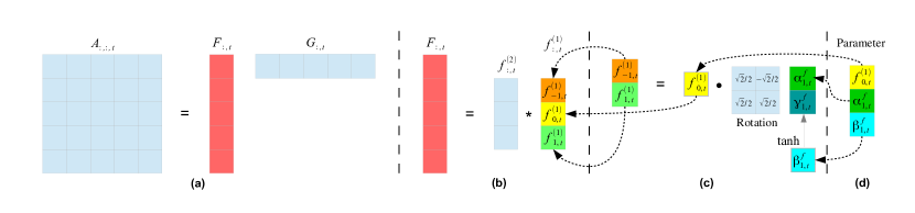
Figure 4: For each channel $t$, (a) the two-dimensional filter $\mathcal{A}_{\bm{:},\bm{:},t}$ is parameterized through an outer product of two 1D-filters $F_{\bm{:},t}$ and $G_{\bm{:},t}$; (b) $F_{\bm{:},t}$ is parameterized through a convolution of $f^{(1)}_{\bm{:},t}\ast\cdots\ast f^{(Q)}_{\bm{:},t}$, and similarly $G_{\bm{:},t}$ as a convolution of $g^{(1)}_{\bm{:},t}\ast\cdots\ast g^{(Q)}_{\bm{:},t}$; (c) we re-parameterize each constrained $(f^{(q)}_{-1,t},f^{(q)}_{1,t})$ to unconstrained $(\alpha^{f}_{q,t},\beta^{f}_{q,t})$, and similarly $(g^{(q)}_{-1,t},g^{(q)}_{1,t})$ to $(\alpha^{g}_{q,t},\beta^{g}_{q,t})$; (d) final parameters for unconstrained optimization are $(\alpha^{f}_{q,t},\beta^{f}_{q,t},\alpha^{g}_{q,t},\beta^{g}_{q,t})_{q=1}^{Q}$.

Theorem 6 (Constraints for Stable Separable ARMA Layer).

A sufficient condition for the separable ARMA layer (Definition 5) to be stable (i.e. output be bounded for any bounded input) is:

$$\left|f^{(q)}_{-1,t}+f^{(q)}_{1,t}\right|<f^{(q)}_{0,t},\leavevmode\nobreak\ \left|g^{(q)}_{-1,t}+g^{(q)}_{1,t}\right|<g^{(q)}_{0,t},\leavevmode\nobreak\ \forall q\in[Q],t\in[T].$$ (7)

The proof is deferred to Appendix D, which follows the standard techniques using Z-transform.

5.2 Achieving stability via re-parameterization

In principle, the constraints required for stability in a ARMA layer as in Theorem 6 could be enforced through constrained optimization. However, constrained optimization algorithm, such as projected gradient descent [2], is more expensive as it requires an extra projection step. Moreover, it could be more difficult to achieve convergence. In order to avoid the aforementioned challenges, we introduce a re-parameterization mechanism to remove constraints needed to guarantee stability in ARMA layer.

Theorem 7 (Re-parameterization).

For a separable ARMA layer in Definition 5, if we re-parameterize each tuple $(f^{(q)}_{-1,t},f^{(q)}_{1,t},g^{(q)}_{-1,t},g^{(q)}_{1,t})$ as learnable parameters $(\alpha^{f}_{q,t},\beta^{f}_{q,t},\alpha^{g}_{q,t},\beta^{g}_{q,t})$:

$$\begin{pmatrix}f^{(q)}_{-1,t}&g^{(q)}_{-1,t}\\ f^{(q)}_{1,t}&g^{(q)}_{1,t}\end{pmatrix}=\begin{pmatrix}f^{(q)}_{0,t}&0\\ 0&g^{(q)}_{0,t}\end{pmatrix}\begin{pmatrix}\sqrt{2}/2&-\sqrt{2}/2\\ \sqrt{2}/2&\sqrt{2}/2\end{pmatrix}\begin{pmatrix}\alpha^{f}_{q,t}&\alpha^{g}_{q,t}\\ \tanh(\beta^{f}_{q,t})&\tanh(\beta^{g}_{q,t})\end{pmatrix}$$ (8)

then the layer is stable for arbitrary $\{(f^{(q)}_{0,t},g^{(q)}_{0,t},\alpha^{f}_{q,t},\beta^{f}_{q,t},\alpha^{g}_{q,t},\beta^{g}_{q,t})_{q=1}^{Q}\}_{t=1}^{T}$ with no constraints.

In practice, we can set $f^{q}_{0,t}=g^{q}_{0,t}=1$ (since the scale can be learned by the moving-average kernel), and only store and optimize over each tuple $(\alpha^{f}_{q,t},\beta^{f}_{q,t},\alpha^{g}_{q,t},\beta^{g}_{q,t})$. In other words, each autoregressive filter $\mathcal{A}_{\bm{:},\bm{:},t}$ is constructed from $(\alpha^{f}_{q,t},\beta^{f}_{q,t},\alpha^{g}_{q,t},\beta^{g}_{q,t})_{q=1}^{Q}$ on the fly during training or inference.

Figure 5: Learning curves with and without re-parameterization on an ARMA network with a VGG-11 backbone on CIFAR-10.

Experimental Demonstration of Re-parameterization. To verify the re-parameterization is essential for stable training, we train a VGG-11 network [30] on CIFAR-10 dataset, where all convolutional layers are replaced by ARMA layers with autoregressive coefficients initialized as zeros. We compare the learning curves using the re-parameterization v.s. not using the re-parameterization in Figure 5. As we can see, the training quickly converges under our proposed re-parameterization mechanism with which the stability of the network is guaranteed. However without the re-parameterization mechanism, a naive training of ARMA network never converges and gets NaN error quickly. The experiment thus verifies that the theory in Theorem 7 is effective in guaranteeing stability.

6 Experiments

We apply our ARMA networks on two dense prediction problems – pixel-level video prediction and semantic segmentation to demonstrate effectiveness of ARMA networks. (1) We incorporate our ARMA layers in U-Net [29, 35] for semantic segmentation, and in ConvLSTM network [38, 5] for video prediction. We show that the resulted ARMA U-Net and ARMA-LSTM models uniformly outperform the baselines on both tasks. (2) We then interpret the varying performance of ARMA networks on different tasks by visualizing the histograms of the learned autoregressive coefficients. We include the detailed setups (datasets, model architectures, training strategies and evaluation metrics) and visualization in Appendix A for reproducibility purposes.

Semantic Segmentation on Biomedical Medical Images. We evaluate our ARMA U-Net on the lesion segmentation task in ISIC 2018 challenge [37], comparing against a baseline U-Net [29] and non-local U-Net [35] (U-Net augmented with non-local attention blocks).

Table 2: Semantic segmentation on ISIC dataset. For all metrics (ACC, SE, SP, PC, F1 and JS), higher values indicates better performance. The reported numbers are an average of $10$ runs with different seeds.

Model	params.	ACC	SE	SP	PC	F1	JS
U-Net [29]	3.453M	0.946 $\pm$ 0.003	0.884 $\pm$ 0.019	0.977 $\pm$ 0.005	0.857 $\pm$ 0.020	0.842 $\pm$ 0.009	0.754 $\pm$ 0.011
NL U-Net [35]	4.403M	0.945 $\pm$ 0.003	0.877 $\pm$ 0.017	0.973 $\pm$ 0.004	0.844 $\pm$ 0.014	0.831 $\pm$ 0.012	0.741 $\pm$ 0.013
ARMA U-Net	3.455M	0.955 $\pm$ 0.003	0.896 $\pm$ 0.011	0.972 $\pm$ 0.005	0.873 $\pm$ 0.011	0.861 $\pm$ 0.007	0.780 $\pm$ 0.009
NL ARMA U-Net	4.405M	0.960 $\pm$ 0.002	0.909 $\pm$ 0.009	0.968 $\pm$ 0.004	0.870 $\pm$ 0.011	0.870 $\pm$ 0.006	0.790 $\pm$ 0.008

ARMA networks outperform both baselines in almost all metrics. As shown in Table 2, our (non-local) ARMA U-Net outperform both U-Net and non-local U-Net except for specificity (SP). Furthermore, we find that the synergy of non-local attention and ARMA layers achieves best results among all.

Pixel-level Video Prediction. We evaluate our ARMA-LSTM network on the Moving-MNIST-2 dataset [11] with different moving velocities, comparing against the baseline ConvLSTM network [38, 5] and its augmentation using dilated convolutions and non-local attention blocks [33]. As shown in the visualizations in Appendix A, the dilated ARMA-LSTM does not have gridding artifacts as in dilated Conv-LSTM, that is ARMA removes the gridding artifacts.

Table 3: 10-frames video prediction on Moving-MNIST-2 with three different speeds (results averaged over 10 predicted frames). MA and AR denote the size of moving-average and autoregressive kernels respectively, and dil. denotes dilation in the moving-average kernel. Higher PSNR, SSIM values indicate better performance.

Model	MA	AR	dil.	params.	original speed		2X speed		3X speed
					PSNR	SSIM	PSNR	SSIM	PSNR	SSIM
Conv-LSTM (size 3)	3	1	1	0.887M	18.24	0.867	16.62	0.827	15.81	0.810
Conv-LSTM (size 5)	5	1	1	2.462M	19.58	0.901	17.61	0.856	16.99	0.841
Dilated Conv-LSTM	3	2	2	0.887M	19.16	0.893	17.92	0.858	17.48	0.846
Dilated ARMA-LSTM	3	3	2	0.893M	19.72	0.904	18.05	0.870	17.65	0.855
ARMA-LSTM (size 3)	3	2	1	0.893M	19.72	0.899	18.73	0.881	18.13	0.869

ARMA networks outperforms larger networks: As shown in Table 3, our ARMA networks with kernel sizes $3\times 3$ outperform all baselines under all velocities (at the original speed, our ARMA network requires dilated convolutions to achieve the best performance). Moreover, for videos with a higher moving speed, the advantage is more pronounced as expected due to ARMA’s ability to expand the ERF. The ARMA networks improve the best baseline (Conv-LSTM with kernel size $5\times 5$) in PSNR by $6.36\%$ at 2X speed and by $6.70\%$ at 3X speed, with 63.7% fewer parameters.

ARMA networks outperforms non-local attention blocks: As shown in Table 4, our ARMA-LSTM with kernel sizes $3\times 3$ outperforms the Conv-LSTMs augmented by non-local attention blocks. However, attention mechanism does not always improve the baselines or our models. When both ARMA-LSTM and Conv-LSTM are combined with non-local attention blocks, our model achieves better performance compared to the non-ARMA baselines.

Table 4: Comparison with non-local attention blocks on video prediction. The original networks are the same as in Table 3. Each non-local network additionally inserts two non-local blocks in the corresponding base network.

Model	Original		Non-local
	PSNR	SSIM	PSNR	SSIM
ConvLSTM (size 3)	18.24	0.867	19.45	0.895
ConvLSTM (size 5)	19.58	0.901	19.18	0.891
ARMA-LSTM (size 3)	19.72	0.899	19.62	0.897

Figure 6: Histogram of the autoregressive coefficients in trained ARMA networks.

Interpretation by Autoregressive Coefficients. To explain why ARMA networks achieve impressive performance in dense prediction, Figure 6 compares the histograms of the trained autoregressive coefficients between video prediction and image classification. (subsection A.4 demonstrates performance of image classifications when ARMA layers are incorporated in VGG and ResNet.)

1. The histograms demonstrate how ARMA networks adaptively learn autoregressive coefficients according to the tasks. As motivated in the introduction, dense prediction such as video prediction requires each layer to have a large receptive field such that global information is captured.

2. The large autoregressive coefficients in video prediction model suggests the overall ERF is significantly expanded. In image classification model, global information is already aggregated by pooling (downsampling) layers and a fully-connected classification layer. Therefore, the ARMA layers automatically learn nearly zero autoregressive coefficients.

7 Discussion

This paper proposes a novel ARMA layer capable of expanding a network’s effective receptive field adaptively. Our method is related to techniques in signal processing and machine learning. First, ARMA layer is equivalent to a multi-channel impulse response filter in signal processing [28]. Alternatively, we can interpret the autoregressive layer as a a learnable spectral normalization [25] following the moving-average layer. Additionally, the ARMA layer is an linear recurrent neural network, where the recurrent propagations are over the spatial domain (section 2).

Appendix of ARMA Nets:
Expanding Receptive Field for Dense Prediction

Appendix A Supplementary Materials for Experiments

In this section, we explain detailed setups (datasets, model architectures, learning strategies and evaluation metrics) of all experiments, and provide additional visualizations of the results.

A.1 Visualization of Effective Receptive Field

In the simulations in subsection 3.2, all linear networks have $32$ channels and $64\times 64$ feature size at each layer. The filter size for both moving-average coefficients and autoregressive coefficients is set to $3\times 3$: each moving-average kernel $\mathcal{W}$ is initialized using Xavier’s method, while the autoregressive kernel $\mathcal{A}$ is initialized randomly within a stable region $-a\leq f^{(q)}_{-1,t}+f^{(q)}_{1,t}\leq 0,-a\leq g^{(q)}_{-1,t}+g^{(q)}_{1,t}\leq 0,\forall t\in[T],q\in[Q]$ (see section 5 for details). Each heat map in Figure 3 is computed as an average of $32$ gradient maps from different channels.

A.2 Multi-frame Video Prediction

Datasets and Metrics

The Moving-MNIST-2 dataset is generated by moving two digits of size $28\times 28$ in MNIST dataset within a $64\times 64$ black canvas [11]. These digits are placed at a random initial location, and move with constant velocity in the canvas and bounce when they reach the boundary. In addition to the default velocity in the public generator [11], we increase the velocity to $2\times$ and $3\times$ to test all models on videos with stronger motions. For each velocity, we generate 10,000 videos for training set, 3,000 for validation set, and 5,000 for test set, where each video contains $20$ frames. All models are trained to the next 10 frames given 10 input frames, and we evaluate their performance based on the metrics of mean square error (MSE), peak signal-noise ratio (PSNR) and structure similarity (SSIM) [36].

Model Architectures

(1) Baselines. The backbone architecture consists of a stack of 12 Conv-LSTM modules, and each module contains 32 units (channels). Following [5], two skip connections that perform channel concatenation are added between (3, 9) and (6, 12) module. An additional traditional convolutional layer is applied on top of all recurrent layers to compute the predicted frames. The backbone architecture is illustrated in Figure 7. In the baseline networks, we consider three different convolutions at each layer: (a) Traditional convolution with filter size $3\times 3$; (b) Traditional convolution with filter size $5\times 5$; and (c) $2$-dilated convolution with filter size $3\times 3$.

(2) ARMA networks. Our ARMA networks use the same backbone architecture as baselines, but replace their convolutional layers with ARMA layers. For all ARMA models, we set the filter size for both moving-average and autoregressive parts to $3\times 3$. In the ARMA networks, we consider two different convolutions each layer: (a) The moving-average part is a traditional convolution; (b) We further consider using $2$-dilated convolution in the moving-average part.

(3) Non-local networks. In non-local networks, we additionally insert two non-local block in the backbone architecture, as illustrated in Figure 8. In each non-local block, we use embedded Gaussian as the non-local operation [33], and we replace the batch normalization by instance normalization that is compatible to recurrent neural networks. In non-local networks, we consider three types of convolutions at each layer: (1)(2) Traditional convolutions with filter size $3\times 3$ and $5\times 5$; (3) ARMA layer with $3\times 3$ moving-average and autoregressive filters.

Figure 7: Conv(ARMA)-LSTM.

Figure 8: Non-Local Conv(ARMA)-LSTM.

Training Strategy

All models are trained using ADAM optimizer [17], with $\mathcal{L}_{1}+\mathcal{L}_{2}$ loss and for $500$ epochs. We set the initial learning rate to $10^{-3}$, and the value for gradient clipping to $3$. Learning rate decay and scheduled sampling [1] are used to ease training. Scheduled sampling is started once the model does not improve in $20$ epochs (in term of validation loss), and the sampling ratio is decreased linearly by $4\times 10^{-4}$ each epoch (i.e. scheduling sampling lasts for $250$ epochs). Learning rate decay is further activated if the validation loss does not drop in 20 epochs, and the learning rate is decreased exponentially by $0.98$ every $5$ epochs. All convolutional layers and moving-average parts in ARMA layers are initialized by Xavier’s normalized initializer [12], and autoregressive coefficients in ARMA layers are initialized as zeros (i.e. each ARMA layer is initialized as a traditional layer).

Visualization of the Predictions

We visualize the predictions by different models under three moving velocites in Figure 9, Figure 10 and Figure 11 Notice that the gridding artifacts by dilated convolutions are removed by ARMA layer: since each neuron receives information from all pixels in a local region (2(d)), adjacent neurons are on longer computed from separate sets of pixels. Moreover, for videos with a higher moving speed, the advantage of our ARMA layer is more pronounced as expected due to ARMA’s ability to expand the ERF.

input	ground truth (top) / predictions
$t=1\;\;\;\;\;\;\;\;\;\;2\;\;\;\;\;\;\;\;\;3$	$4\;\;\;\;\;\;\;\;\;\;\;5\;\;\;\;\;\;\;\;\;\;6\;\;\;\;\;\;\;\;\;\;\;7\;\;\;\;\;\;\;\;\;\;\;\;8\;\;\;\;\;\;\;\;\;9\;\;\;\;\;\;\;\;\;10\;\;\;\;\;\;\;\;\;11\;\;\;\;\;\;\;\;\;12\;\;\;\;\;\;\;\;\;\;13$
Traditional ($K_{w}=3$)
$2$-dilated ($K_{w}=3$)
Traditional ($K_{w}=5$)
$2$-dilated ARMA ($K_{w}=3,K_{a}=3$)
ARMA ($K_{w}=3,K_{a}=3$)

Figure 9: Prediction on Moving-MNIST-2 (original speed). The first row contains the last $3$ input frames and $10$ ground-truth frames for models to predict.

input	ground truth (top) / predictions
$t=1\;\;\;\;\;\;\;\;\;\;2\;\;\;\;\;\;\;\;\;3$	$4\;\;\;\;\;\;\;\;\;\;\;5\;\;\;\;\;\;\;\;\;\;6\;\;\;\;\;\;\;\;\;\;\;7\;\;\;\;\;\;\;\;\;\;\;\;8\;\;\;\;\;\;\;\;\;9\;\;\;\;\;\;\;\;\;10\;\;\;\;\;\;\;\;\;11\;\;\;\;\;\;\;\;\;12\;\;\;\;\;\;\;\;\;\;13$
Traditional ($K_{w}=3$)
$2$-dilated ($K_{w}=3$)
Traditional ($K_{w}=5$)
$2$-dilated ARMA ($K_{w}=3,K_{a}=3$)
ARMA ($K_{w}=3,K_{a}=3$)

Figure 10: Prediction on Moving-MNIST-2 ($2\times$ speed). The first row contains the last $3$ input frames and $10$ ground-truth frames for models to predict.

input	ground truth (top) / predictions
$t=1\;\;\;\;\;\;\;\;\;\;2\;\;\;\;\;\;\;\;\;3$	$4\;\;\;\;\;\;\;\;\;\;\;5\;\;\;\;\;\;\;\;\;\;6\;\;\;\;\;\;\;\;\;\;\;7\;\;\;\;\;\;\;\;\;\;\;\;8\;\;\;\;\;\;\;\;\;9\;\;\;\;\;\;\;\;\;10\;\;\;\;\;\;\;\;\;11\;\;\;\;\;\;\;\;\;12\;\;\;\;\;\;\;\;\;\;13$
Traditional ($K_{w}=3$)
$2$-dilated ($K_{w}=3$)
Traditional ($K_{w}=5$)
$2$-dilated ARMA ($K_{w}=3,K_{a}=3$)
ARMA ($K_{w}=3,K_{a}=3$)

Figure 11: Prediction on Moving-MNIST-2 ($3\times$ speed). The first row contains the last $3$ input frames and $10$ ground-truth frames for models to predict.

(a) MSE

(b) PSNR

(c) SSIM

Figure 12: Per-frame performance comparison of our ARMA and our dilated ARMA networks v.s. the Conv-LSTM, dilated Conv-LSTM baselines for Moving-MNIST-2 (original speed). Lower MSE values (in $10^{-3}$) or higher PSNR/SSIM values indicate better performance.

(a) MSE

(b) PSNR

(c) SSIM

Figure 13: Per-frame performance comparison of our ARMA and our dilated ARMA networks v.s. the Conv-LSTM, dilated Conv-LSTM baselines for Moving-MNIST-2 ($2\times$ speed). Lower MSE values (in $10^{-3}$) or higher PSNR/SSIM values indicate better performance.

(a) MSE

(b) PSNR

(c) SSIM

Figure 14: Per-frame performance comparison of our ARMA and our dilated ARMA networks v.s. the Conv-LSTM, dilated Conv-LSTM baselines for Moving-MNIST-2 ($3\times$ speed). Lower MSE values (in $10^{-3}$) or higher PSNR/SSIM values indicate better performance.

A.3 Medical Image Segmentation

To demonstrate ARMA networks’ applicability to image segmentation, we evaluate it on a challenging medical image segmentation problem.

Dataset and Metrics

For all experiments, we use a dataset from ISIC 2018: Skin Lesion Analysis Towards Melanoma Detection [8], which can be downloaded online. In this task, a model aims to predict a binary mask that indicates the location of the primary skin lesion for each input image. The dataset consists of $2594$ images, and we resize each image to $224\times 224$. We split dataset into training set, validation set and test set with ratios of $0.7$, $0.1$ and $0.2$ respectively. All models are evaluated using the following metrics: $AC=(TP+TN)/(TP+TN+FP+FN)$, $SE=TP/(TP+FN)$, $SP=TN/(TN+FP)$, $PC=TP/(TP+FP)$, $F1=2PC\cdot SE/(PC+SE)$ and $JS=|GT\cap SR|/|GT\cup SR|$, where TP stands for true positive, TN for true negative, FP for false positive, FN for false negative, GT for ground truth mask and SR for predictive mask.

Model Architectures

(1) Baselines. We use U-Net [29] and non-local U-Net [35] as baseline models. U-Net has a contracting path to capture context and a symmetric expanding path enables precise localization. The network architecture is illustrated in 15(a). Non-local U-Net is equipped with global aggregation blocks based on the self-attention operator to aggregate global information without a deep encoder for biomedical image segmentation, which is illustrated in 15(b). (2) Our architectures. We replace all traditional convolution layers with ARMA layers in U-Net and non-local U-Net.

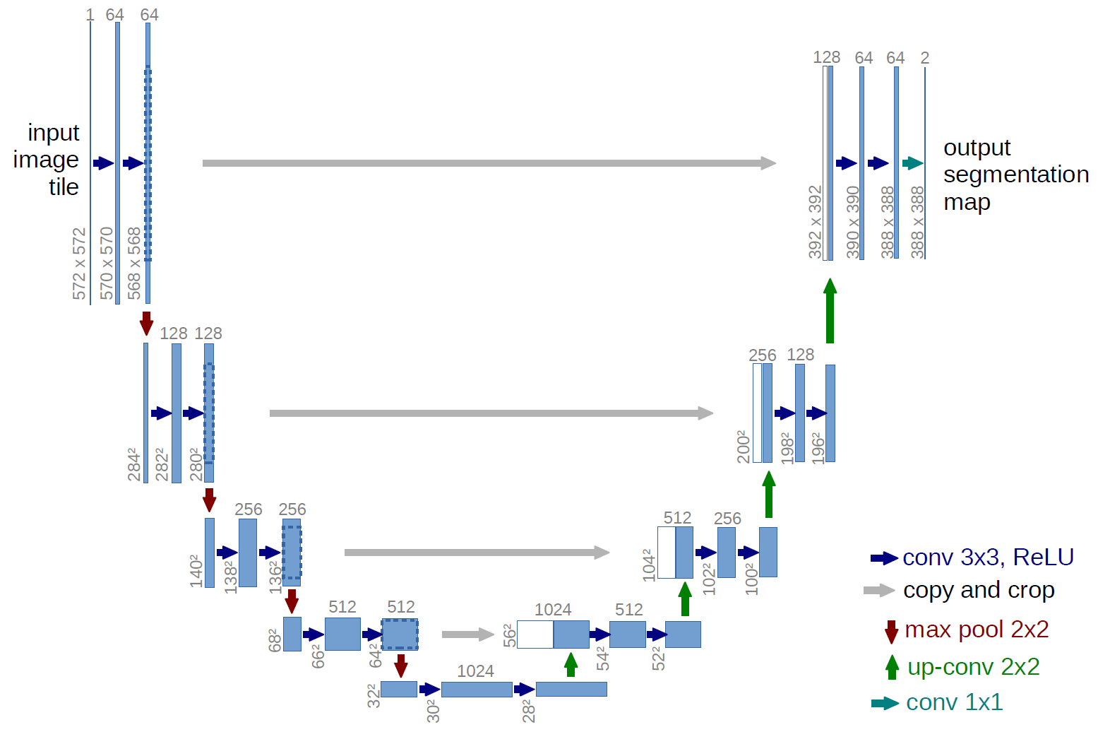
(a) U-Net architecture.

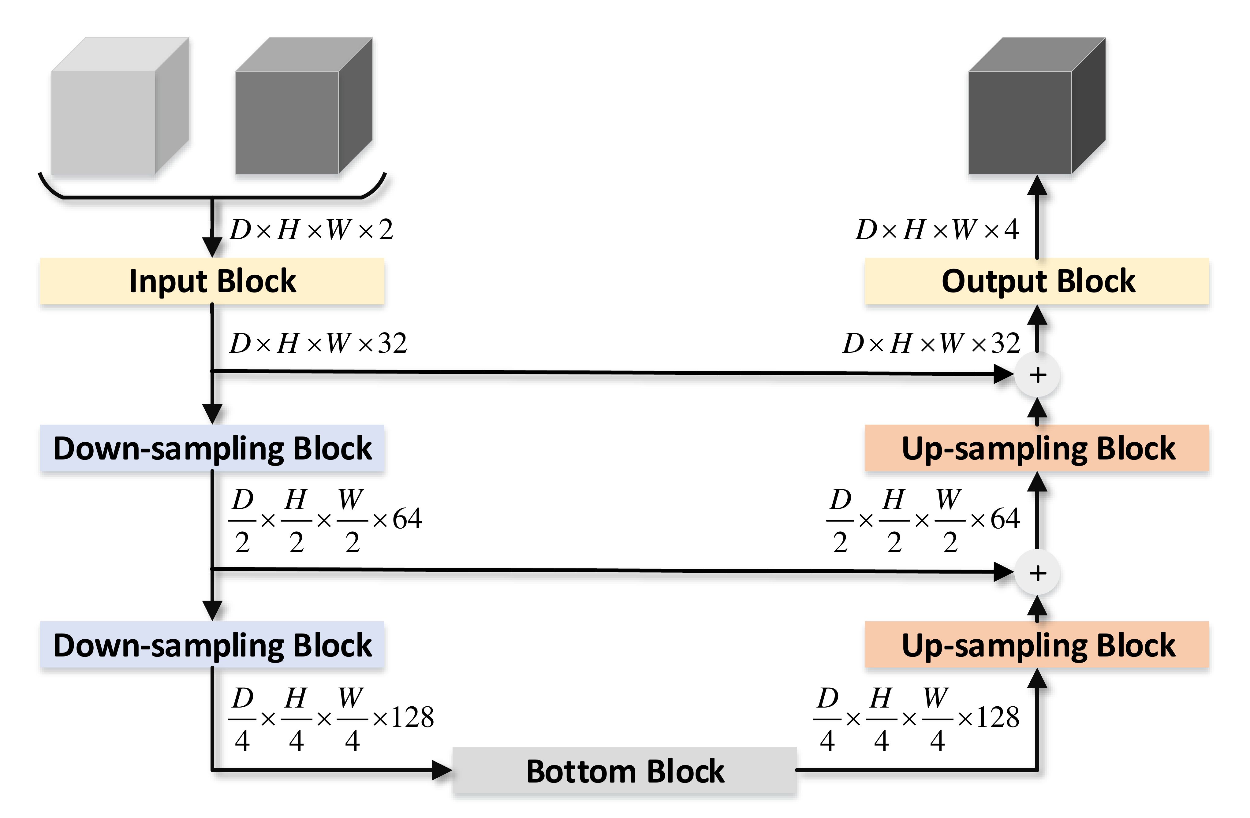
(b) Non-local U-Net architecture.

Figure 15: Backbone architectures.

Training Strategy.

All models are trained using ADAM optimizer [17] with binary cross entropy (BCE) loss. For initial learning rate, we search from $10^{-2}$ to $10^{-5}$ and choose $10^{-3}$ for U-Net and $10^{-2}$ for non-local U-Net. The learning rate is decayed by $0.98$ every epoch. During training, each image is randomly augmented by rotation, cropping, shifting, color jitter and normalization following the public source code.

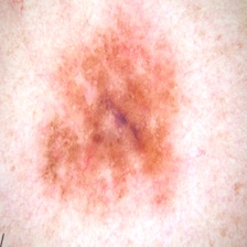
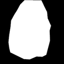
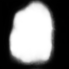
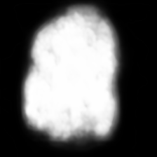
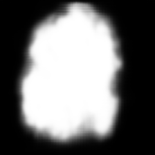
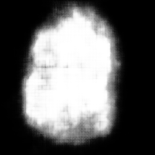
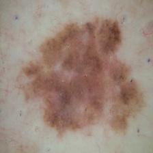
Input

image

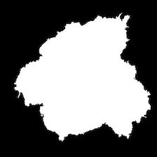
Ground

truth

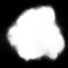
U-net

with ARMA

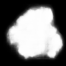
U-net

without ARMA

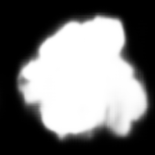
Non-Local U-net

with ARMA

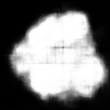
Non-Local U-net

without ARMA

Figure 16: Predictive results of U-Net and Non-local U-Net with/without ARMA layers.

A.4 Image Classification

Model Architectures and Datasets

We replace the traditional convolutional layers by ARMA layers in three benchmarking architectures for image classification: AlexNet [18], VGG-11 [30], and ResNet-18 [13]. We apply our proposed ARMA networks on CIFAR10 and CIFAR100 datasets. Both datasets have $50000$ training examples and $10000$ test examples, and we use $5000$ examples from the training set for validation (and leave $45000$ examples for training).

Training Strategy

All models are trained using cross-entropy loss and SGD optimizer with batch size $128$, learning rate $0.1$, weight decay $0.0005$ and momentum $0.9$. For CIFAR10, the models are trained for $300$ epochs and we half the learning rate every $30$ epochs. For CIFAR100, the models are trained for $200$ epochs and we divide the learning rate by 5 at the $60^{\text{th}}$, $120^{\text{th}}$, $160^{\text{th}}$ epochs.

Results

The experimental results are summarized in Table 5. Our results show that ARMA models achieve comparable or slightly better results than the benchmarking architectures. Replacing traditional convolutional layer with our proposed ARMA layer slightly boosts the performance of VGG-11 and ResNet-18 by 0.01%-0.1% in accuracy. Since image classifications tasks do not require convolutional layers to have large receptive field, the learned autoregressive coefficients are highly concentrated around 0 as shown in Figure 6. Consequently, ARMA networks effectively reduce to traditional convolutional neural networks and therefore achieve comparable results.

	AlexNet		VGG-11		ResNet-18
	Conv.	ARMA	Conv.	ARMA	Conv.	ARMA
CIFAR10	$86.30\pm 0.29$	$85.67\pm 0.19$	$91.57\pm 0.59$	$91.57\pm 0.73$	$95.01\pm 0.15$	$95.07\pm 0.13$
CIFAR100	$58.99\pm 0.37$	$57.43\pm 0.24$	$68.25\pm 0.11$	$68.36\pm 1.67$	$73.71\pm 0.23$	$73.72\pm 0.52$

Table 5: Image classification on CIFAR10 and CIFAR100. The reported accuracies (%) and their standard deviations are computed from $10$ runs with different seeds. Since image classifications tasks do not require convolutional layers to have large receptive field, the learned autoregressive coefficients are highly concentrated around $0$ as shown in Figure 6. Consequently, ARMA networks effectively reduce to traditional CNNs and therefore achieve comparable results.

Appendix B Analysis of Effective Receptive Field (ERF)

In this section, we prove the Theorem 3 in subsection 3.2. Throughout this section, we use $\bm{a}^{(\ell)}=\{\cdots,a^{(\ell)}_{-1},a^{(\ell)}_{0},a^{(\ell)}_{1},\cdots\}$ to denote the $\ell^{\text{th}}$ layer’s autoregressive coefficients, and $\bm{w}^{(\ell)}=\{\cdots,w^{(\ell)}_{-1},w^{(\ell)}_{0},w^{(\ell)}_{1},\cdots\}$ the $\ell^{\text{th}}$ layer’s autoregressive coefficients.

B.1 ERF of General Linear Convolutional Networks

The proof of is Theorem 3 based on the following theorem on linear convolutional networks [24], which includes both CNN and ARMA networks as special cases.

Theorem 8 (ERF of linear convolutional networks with infinite horizon).

Consider an $L$-layer linear convolutional network (without activation and pooling), where its $\ell^{\text{th}}$-layer computes a weighted-sum of its input $y^{(\ell)}_{i}=\sum_{p=-\infty}^{+\infty}w^{(\ell)}_{p}y^{(\ell-1)}_{i-p}$. Suppose the weights are non-negative $w^{(\ell)}_{p}\geq 0$ and normalized at each layer $\sum_{p=-\infty}^{+\infty}w^{(\ell)}_{p}=1,1\leq\ell\leq[L]$, the network has an ERF radius as

$$r^{2}(\text{ERF})=\sum_{\ell=1}^{L}\left[\sum_{p=-\infty}^{+\infty}p^{2}w^{(\ell)}_{p}-\left(\sum_{p=-\infty}^{+\infty}pw^{(\ell)}_{p}\right)^{2}\right]$$ (B.1)

Furthermore, the ERF converges to a Gaussian density function when $L$ tends to infinity.

Proof.

In this linear convolutional network, the gradient maps can be computed with chain rule as

$$g_{i,\bm{:}}={\bm{w}^{(1)}}^{\top}\ast{\bm{w}^{(2)}}^{\top}\cdots\ast{\bm{w}^{(L)}}^{\top},\leavevmode\nobreak\ \forall i\in\mathbb{Z}$$ (B.2)

where ${w}^{\ell\top}$ denotes the reversed sequence of $\bm{w}^{(\ell)}$. Notice that (1) The gradient maps do not depend on the input, i.e. they are data-independent; (2) The gradient maps are identical across different locations in the output. Consequently, the ERF is equal to any one gradient map above

$$\text{ERF}={\bm{w}^{(1)}}^{\top}\ast{\bm{w}^{(2)}}^{\top}\cdots\ast{\bm{w}^{(L)}}^{\top}$$ (B.3)

The remaining part of the proof makes use of probabilistic method, which interprets the operation at each layer as a discrete random variable. Since the weights at each layer are non-negative and normalized, they can be treated as values of a probability mass function. Concretely, we construct $L$ independent random variables $\{{W}^{(1)},\cdots,{W}^{(L)}\}$ such that $\mathbb{P}[{W}^{(\ell)}=p]=w^{(\ell)}_{-p}$. Similarly, we introduce a random variable ${S}^{(L)}$ to represent the ERF, i.e. $\mathbb{P}[{S}^{(L)}=p]=\text{ERF}_{p}$. As a result, the ERF radius is equal to standard deviation of ${S}^{(L)}$, or equivalently $r^{2}(\text{ERF})=\mathbb{V}[{S}^{(L)}]$.

Recall that addition of independent random variables results in convolution of their probability mass functions, Equation B.3 implies that ${S}^{(L)}$ is an addition of all ${W}^{(\ell)}$’s, i.e. ${S}^{(L)}=\sum_{\ell=1}^{L}{W}^{(\ell)}$. Therefore, the variance of ${S}^{(L)}$ is equal to a summation of the variances for ${W}^{(\ell)}$’s. Thus,

$$\mathbb{V}[{S}^{(L)}] =\sum_{\ell=1}^{L}\mathbb{V}[{W}^{(\ell)}]=\sum_{\ell=1}^{L}\left[\mathbb{E}[({W}^{(\ell)})^{2}]-\mathbb{E}[{W}^{(\ell)}]^{2}\right]$$ (B.4)

$$=\sum_{\ell=1}^{L}\left[\sum_{p=-\infty}^{+\infty}p^{2}w^{(\ell)}_{p}-\left(\sum_{p=-\infty}^{+\infty}pw^{(\ell)}_{p}\right)^{2}\right]$$ (B.5)

which proves the Equation B.1. Furthermore, the Lyapunov central limit theorem shows that $({S}^{(L)}-\mathbb{E}[{S}^{(L)}])/\mathbb{V}[{S}^{(L)}]$ converges to a standard normal random variable if $L$ tends to infinity

$$\frac{{S}^{(L)}-\mathbb{E}[{S}^{(L)}]}{\sqrt{\mathbb{V}[{S}^{(L)}]}}=\frac{\sum_{\ell=1}^{L}\left({W}^{(\ell)}-\mathbb{E}[{W}^{(\ell)}]\right)}{\sqrt{\sum_{\ell=1}^{L}\mathbb{V}[{W}^{(\ell)}]}}\xrightarrow[]{D}\mathcal{N}(0,1)$$ (B.6)

that is, the ERF function is approximately Gaussian when the number of layers $L$ is large enough. ∎

B.2 ERF of Traditional CNNs ($a^{(\ell)}_{1}=-{a}^{(\ell)}=0$)

As a warmup, we first provide a proof for the special case of traditional CNN where ${a}^{(\ell)}=0$ for all layers. For reference, we list the first two cases of Faulhaber’s formula:

$$\sum_{p=0}^{K-1}p=\frac{K(K-1)}{2}$$ (B.7a)

$$\sum_{p=0}^{K-1}p^{2}=\frac{K(K-1)(2K-1)}{6}$$ (B.7b)

Proof.

In this special case, the ERF radius can be obtained by plugging $w^{(\ell)}_{p}=1/{K}^{(\ell)}$ for $p=0,{d}^{(\ell)},\cdots,{d}^{(\ell)}({K}^{(\ell)}-1)$ into Equation B.1.

$$r^{2}(\text{ERF}) =\sum_{\ell=1}^{L}\left[\sum_{p=0}^{{K}^{(\ell)}-1}\frac{\left(p{d}^{(\ell)}\right)^{2}}{{K}^{(\ell)}}-\left(\sum_{p=0}^{{K}^{(\ell)}-1}\frac{p{d}^{(\ell)}}{{K}^{(\ell)}}\right)^{2}\right]$$ (B.8)

$$=\sum_{\ell=1}^{L}\left[\frac{{{d}^{(\ell)}}^{2}}{{K}^{(\ell)}}\frac{{K}^{(\ell)}\left({K}^{(\ell)}-1\right)\left(2{K}^{(\ell)}-1\right)}{6}-\left(\frac{{d}^{(\ell)}}{{K}^{(\ell)}}\frac{{K}^{(\ell)}\left({K}^{(\ell)}-1\right)}{2}\right)^{2}\right]$$ (B.9)

$$=\sum_{\ell=1}^{L}\frac{{{{d}^{(\ell)}}^{2}}\left({{K}^{(\ell)}}^{2}-1\right)}{12}$$ (B.10)

where the infinite series are computed using Equation B.7a and Equation B.7b. Taking square root on both sides completes the proof for the special case of CNNs. ∎

ERF Analysis of CNNs. If we further assume that all layers are identical, i.e. ${K}^{(\ell)}=K,{d}^{(\ell)}=d$ for $1\leq\ell\leq L$, we can simplify Equation B.10 as

$$r(\text{ERF})=\sqrt{L}\cdot\sqrt{\frac{d^{2}(K^{2}-1)}{12}}=O\left(dK\sqrt{L}\right)$$ (B.11)

That is, the ERF radius grows linearly with kernel size $K$ and dilation $d$, but sub-linearly with the number of layers $L$ in the linear network.

B.3 ERF of ARMA networks ($a^{(\ell)}_{1}=-{a}^{(\ell)}\leq 0$)

In the part, we provide a proof for general ARMA networks where ${a}^{(\ell)}\leq 0$. In sketch, the proof consists of three steps: (1) we introduce inverse convolution and convert each ARMA model to a moving-average model: $\bm{a}\ast\bm{y}=\bm{w}\ast\bm{x}\implies\bm{y}=\bm{f}\ast\bm{x}$, where $\bm{f}$ represents a convolution with infinite number of coefficients, $\bm{x}$ and $\bm{y}$ are the input and output of the model respectively. (2) We derive the moment generating function (MGF) of the moving-average coefficients from the first step, and use the functions to compute the first and second moments. (3) We plug the moments from the second step into Equation B.1 to obtain Equation 3.

Definition 9 (Inverse convolution).

Given a convolution (with coefficients) $\bm{a}$, its inverse convolution $\overline{\bm{a}}$ is defined such that $\bm{a}\ast\overline{\bm{a}}=\overline{\bm{a}}\ast\bm{a}=\bm{\delta}$ is an identical mapping, i.e.

$$\sum_{p=-\infty}^{+\infty}a_{i-p}\overline{a}_{p}=\delta_{i}=\left\{\begin{aligned} 1\qquad i=0\\ 0\qquad i\neq 0\end{aligned}\right.$$ (B.12)

Remark: The inverse convolution does not exist for any convolution $\bm{a}$. A necessary and sufficient condition for invertibility of $\bm{a}$ is that its Fourier transform is non-zero everywhere [28].

Definition 10 (Moments and Moment Generating Function, MGF).

Given a convolution (with coefficients) $\bm{f}$, its $i^{\text{th}}$ moment is defined as

$$M_{i}(\bm{f})=\sum_{p=-\infty}^{+\infty}f_{p}p^{i}$$ (B.13)

Furthermore, we define the moment generating function of the coefficients $\bm{f}$ as

$$M_{\bm{f}}(\lambda)=\sum_{p=-\infty}^{+\infty}f_{p}e^{\lambda p}$$ (B.14)

The name “moment generating” comes from the fact that

$$M_{i}(\bm{f})=\left.\frac{d^{i}M_{\bm{f}}(\lambda)}{{d\lambda}^{i}}\right\rvert_{\lambda=0}$$ (B.15)

Remark: Since moment generating function (MGF) could be interpreted as a real-valued discrete-time Fourier transform (DTFT), the properties of MGF are very similar to the ones of DTFT. In particular, the convolution theorem also holds for MGF, i.e. $M_{\bm{f}\ast\bm{g}}(\lambda)=M_{\bm{f}}(\lambda)M_{\bm{g}}(\lambda)$. If two convolutions $\bm{a}$ and $\overline{\bm{a}}$ are inverse to each other, we have $M_{\bm{a}}(\lambda)M_{\overline{\bm{a}}}(\lambda)=1$.

Now we are ready to prove Theorem 3 using Theorem 8 and Definitions 9 and 10.

Proof.

Let $\bm{f}^{(\ell)}=\bm{\overline{a}}^{(\ell)}\ast\bm{w}^{(\ell)}$, we have

$$\bm{y}^{(\ell)} =\bm{\delta}\ast\bm{y}^{(\ell)}=\left(\bm{\overline{a}}^{(\ell)}\ast\bm{a}^{(\ell)}\right)\ast\bm{y}^{(\ell)}=\bm{\overline{a}}^{(\ell)}\ast\left(\bm{a}^{(\ell)}\ast\bm{y}^{(\ell)}\right)$$ (B.16)

$$=\bm{\overline{a}}^{(\ell)}\ast\left(\bm{w}^{(\ell)}\ast\bm{y}^{(\ell-1)}\right)=\left(\bm{\overline{a}}^{(\ell)}\ast\bm{w}^{(\ell)}\right)\ast\bm{y}^{(\ell-1)}=\bm{f}^{(\ell)}\ast\bm{y}^{(\ell-1)}$$

where each $\bm{f}^{(\ell)}$ has infinite number of coefficients. We denote the MGF of $\bm{f}^{(\ell)}$ as $M_{\bm{f}^{(\ell)}}$, and its first and second moments as $M_{1}(\bm{f}^{(\ell)})$ and $M_{2}(\bm{f}^{(\ell)})$. With the moments of $\bm{f}^{(\ell)}$, we can rewrite Equation B.1 in Theorem 8 as

$$r^{2}(\text{ERF})=\sum_{\ell=1}^{L}\left[M_{2}(\bm{f}^{(\ell)})-\left(M_{1}(\bm{f}^{(\ell)})\right)^{2}\right]$$ (B.17)

The remaining part is to compute $M_{\bm{f}^{(\ell)}}$ for each $\bm{f}^{(\ell)}$, with which $M_{1}(\bm{f}^{(\ell)})$ and $M_{2}(\bm{f}^{(\ell)})$ are generated. Notice that $\bm{f}^{(\ell)}=\bm{\overline{a}}^{(\ell)}\ast\bm{w}^{(\ell)}$ is a convolution between $\bm{\overline{a}}^{(\ell)}$ and $\bm{w}^{(\ell)}$, we have

$$M_{\bm{f}^{(\ell)}}(\lambda) =M_{\bm{\overline{a}}^{(\ell)}}(\lambda)M_{\bm{w}^{(\ell)}}(\lambda)=\frac{M_{\bm{w}^{(\ell)}}(\lambda)}{M_{\bm{a}^{(\ell)}}(\lambda)}$$ (B.18)

$$=\frac{1}{1-{a}^{(\ell)}e^{\lambda}}\sum_{p=0}^{{K}^{(\ell)}-1}\frac{1-{a}^{(\ell)}}{{K}^{(\ell)}}e^{\lambda p{d}^{(\ell)}}$$ (B.19)

where the first equation uses the property that $M_{\bm{a}^{(\ell)}}(\lambda)M_{\bm{\overline{a}}^{(\ell)}}(\lambda)=1$ for any $\lambda$. The first moment $M_{1}(\bm{f}^{(\ell)})$ is therefore

$$M_{1}(\bm{f}^{(\ell)})=\left.\frac{dM_{\bm{f}^{(\ell)}}(\lambda)}{d\lambda}\right\rvert_{\lambda=0}$$ (B.20)

$$=\leavevmode\nobreak\ \bigg{\{}\frac{{a}^{(\ell)}}{\left(1-{a}^{(\ell)}\lambda\right)^{2}}\sum_{p=0}^{{K}^{(\ell)}}\frac{1-{a}^{(\ell)}}{{K}^{(\ell)}}e^{\lambda p{d}^{(\ell)}}+\frac{1}{1-{a}^{(\ell)}e^{\lambda}}\sum_{p=0}^{{K}^{(\ell)}-1}\frac{1-{a}^{(\ell)}}{{K}^{(\ell)}}p{d}^{(\ell)}e^{\lambda p{d}^{(\ell)}}\bigg{\}}_{\lambda=0}$$ (B.21)

$$=\leavevmode\nobreak\ \frac{{a}^{(\ell)}}{1-{a}^{(\ell)}}+\frac{{d}^{(\ell)}}{{K}^{(\ell)}}\left(\sum_{p=0}^{{K}^{(\ell)}-1}p\right)$$ (B.22)

$$=\leavevmode\nobreak\ \frac{{a}^{(\ell)}}{1-{a}^{(\ell)}}+\frac{{d}^{(\ell)}\left({K}^{(\ell)}-1\right)}{2}$$ (B.23)

where the last equation makes use of Equation B.7a. Similarly, the second moment $M_{2}(\bm{f}^{(\ell)})$ is

$$M_{2}(\bm{f}^{(\ell)})=\left.\frac{d^{2}M_{\bm{f}^{(\ell)}}(\lambda)}{{d\lambda}^{2}}\right\rvert_{\lambda=0}$$ (B.24)

$$=\leavevmode\nobreak\ \begin{aligned} \bigg{\{}\frac{{{a}^{(\ell)}}^{2}}{\left(1-{a}^{(\ell)}\right)^{3}}&\sum_{p=0}^{{K}^{(\ell)}}\frac{1-{a}^{(\ell)}}{{K}^{(\ell)}}e^{\lambda p{d}^{(\ell)}}+\frac{2{a}^{(\ell)}}{\left(1-{a}^{(\ell)}e^{\lambda}\right)^{2}}\sum_{p=0}^{{K}^{(\ell)}-1}\frac{1-{a}^{(\ell)}}{{K}^{(\ell)}}p{d}^{(\ell)}e^{\lambda p{d}^{(\ell)}}\\ &\quad+\frac{1}{1-{a}^{(\ell)}e^{\lambda}}\sum_{p=0}^{{K}^{(\ell)}-1}\frac{1-{a}^{(\ell)}}{{K}^{(\ell)}}\left(p{d}^{(\ell)}\right)^{2}e^{\lambda p{d}^{(\ell)}}\bigg{\}}_{\lambda=0}\end{aligned}$$ (B.25)

$$=\left(\frac{{a}^{(\ell)}}{1-{a}^{(\ell)}}\right)^{2}+\frac{2{a}^{(\ell)}}{1-{a}^{(\ell)}}\frac{{d}^{(\ell)}}{{K}^{(\ell)}}\left(\sum_{p=0}^{{K}^{(\ell)}-1}p\right)+\frac{{{d}^{(\ell)}}^{2}}{{K}^{(\ell)}}\left(\sum_{p=0}^{{K}^{(\ell)}-1}p^{2}\right)$$ (B.26)

$$=\left(\frac{{a}^{(\ell)}}{1-{a}^{(\ell)}}\right)^{2}+\frac{2{a}^{(\ell)}}{1-{a}^{(\ell)}}\frac{{d}^{(\ell)}\left({K}^{(\ell)}-1\right)}{2}+\frac{{{d}^{(\ell)}}^{2}\left({K}^{(\ell)}-1\right)\left(2{K}^{(\ell)}-1\right)}{6}$$ (B.27)

Plugging Equation B.23 and Equation B.27 into Equation B.17, we have

$$r^{2}(\text{ERF})=\sum_{\ell=1}^{L}\left[\frac{{{d}^{(\ell)}}^{2}\left({K}^{(\ell)}-1\right)^{2}}{12}+\frac{{a}^{(\ell)}}{\left(1-{a}^{(\ell)}\right)^{2}}\right]$$ (B.28)

Taking square root on both sides completes the proof. ∎

ERF Analysis of ARMA Networks. If we assume all layers are identical, i.e. ${K}^{(\ell)}=K,{d}^{(\ell)}=d,{a}^{(\ell)}=a$ for $1\leq\ell\leq L$, we can simplify Equation B.28 as

$$r(\text{ERF})=\sqrt{L}\cdot\sqrt{\frac{d^{2}(K^{2}-1)}{12}+\frac{a}{(1-a)^{2}}}=O\left(\sqrt{L}\max\left(dK,\frac{\sqrt{a}}{1-a}\right)\right)$$ (B.29)

The ERF radius is dominated by the AR coefficient when $a\lessapprox 1$ regardless of kernel size $K$ and dilation $d$. The radius still grows sub-linearly with the number of layers $L$ in the linear network.

Appendix C Computation of ARMA Layers

In the section, we first derive the backpropagation rules in Theorem 4. We then show how to efficiently compute both forward and backward passes in ARMA layer using Fast Fourier Transform.

C.1 Backpropagation in ARMA models

In this part, we will prove a general theorem for backpropagation in ARMA models. To keep the notations simple, we derive the backpropagation equations for ARMA models with one dimension input/output and one channel. However, the techniques in the proof can be trivially extended to general ARMA models with high-dimensional input/output with multiple channels.

Theorem 11 (Backpropagation in an ARMA model).

Consider an ARMA model $\bm{a}\ast\bm{y}=\bm{w}\ast\bm{x}$, where $\bm{a}$ and $\bm{w}$ are the sequences of moving-average and autoregressive coefficients respectively, the gradients $\{{\partial\mathcal{L}}/{\partial{\bm{x}}},{\partial\mathcal{L}}/{\partial{\bm{w}}},{\partial\mathcal{L}}/{\partial{\bm{a}}}\}$ can be computed from ${\partial\mathcal{L}}/{\partial{\bm{y}}}$ with the following equations:

$$\bm{a}^{\top}\ast\frac{\partial\mathcal{L}}{\partial{\bm{x}}} =\bm{w}^{\top}\ast\frac{\partial\mathcal{L}}{\partial{\bm{y}}}$$ (C.1a)

$$-\bm{a}^{\top}\ast\frac{\partial\mathcal{L}}{\partial{\bm{a}}} =\bm{y}^{\top}\ast\frac{\partial\mathcal{L}}{\partial{\bm{y}}}$$ (C.1b)

$$\bm{a}^{\top}\ast\frac{\partial\mathcal{L}}{\partial{\bm{w}}} =\bm{x}^{\top}\ast\frac{\partial\mathcal{L}}{\partial{\bm{y}}}$$ (C.1c)

where $\bm{a}^{\top}$, $\bm{w}^{\top}$ and $\bm{y}^{\top}$ denote the reversed sequences of $\bm{a}$, $\bm{w}$ and $\bm{y}$ respectively.

Notice that Theorem 4 is special case of Theorem 11: the first equation in Equation 5 is proved by Equation C.1b, and the second equation is proved by Equation C.1a.

We provide two different proofs of Theorem 11. (1) The analysis in our first proof is based on real numbers, and applicable to arbitrary types of convolution. (2) If the convolution is circular (as in the implementation of this paper), we provide a simpler proof using Fourier transform (therefore complex numbers). The second proof also suggests an FFT-based algorithm to compute the backpropagation in Equation 5 efficiently.

C.1.1 Proof in Real Numbers $\mathbb{R}$

Before we prove the theorem, we first prove a useful lemma on the inverse of transposed convolution.

Lemma 12 (Inverse of transposed convolution).

Given a convolution (with coefficients) $\bm{a}$, the operations of inversion and transposition are exchangeable,

$$\overline{\bm{a}^{\top}}=\overline{\bm{a}^{\top}}$$ (C.2)

that is, the inverse transposed convolution is equal to the transposed inverse convolution.

Proof.

The lemma is an immediate result of the definitions of inverse and transposed convolutions.

$$\sum_{p=-\infty}^{+\infty}a^{\top}_{p}\overline{a}^{\top}_{i-p}=\sum_{p=-\infty}^{+\infty}a_{-p}\overline{a}_{p-i}=\delta_{-i}=\delta_{i}\quad\forall i$$ (C.3)

which shows the inverse of $\bm{a}^{\top}$, i.e. $\overline{\bm{a}^{\top}}$, is equal to $\overline{\bm{a}}^{\top}$. ∎

Now we are ready to prove Theorem 11 at the beginning of this section.

Proof.

To begin with, we write the ARMA model $\bm{a}\ast\bm{y}=\bm{w}\ast\bm{x}$ in its weighted-sum form:

$$\sum_{q=-\infty}^{+\infty}a_{q}y_{i-q}=\sum_{p=-\infty}^{+\infty}w_{p}x_{i-p},\leavevmode\nobreak\ \forall i$$ (C.4)

Taking derivative w.r.t. $a_{r}$ on both sides, and since the right side is a constant w.r.t. $a_{r}$, we have

$$\frac{\partial{\left(\sum_{q=-\infty}^{+\infty}a_{q}y_{q}\right)}}{\partial{a_{r}}}=0,\leavevmode\nobreak\ \forall i,r$$ (C.5)

By implicit function theorem, the left hand side can be further expanded as

$$\frac{\partial{\left(\sum_{q=-\infty}^{+\infty}a_{q}y_{i-q}\right)}}{\partial{a_{r}}}=\sum_{q=-\infty}^{+\infty}\frac{\partial{\left(a_{q}y_{i-q}\right)}}{\partial{a_{r}}}$$ (C.6)

$$=\leavevmode\nobreak\ \sum_{q\neq r}a_{q}\frac{\partial{y_{i-q}}}{\partial{a_{r}}}+\left(y_{i-r}+a_{r}\frac{\partial{y_{i-r}}}{\partial{a_{r}}}\right)$$ (C.7)

$$=\leavevmode\nobreak\ \sum_{q=-\infty}^{+\infty}a_{q}\frac{\partial{y_{i-q}}}{\partial{a_{r}}}+y_{i-r}=0,\leavevmode\nobreak\ \forall i,r$$ (C.8)

Rearranging the equation above, we have

$$-\sum_{q=-\infty}^{+\infty}a_{q}\frac{\partial{y_{i-q}}}{\partial{a_{r}}}=y_{i-r},\leavevmode\nobreak\ \forall i,r$$ (C.9a)

Repeating the procedure twice for the derivatives w.r.t. $$w_{r} x_{r}$$ and , we have two similar equations:

$$\sum_{q=-\infty}^{+\infty}a_{q}\frac{\partial{y_{i-q}}}{\partial{w_{r}}} =x_{i-r},\leavevmode\nobreak\ \forall i,r$$ (C.9b)

$$\sum_{q=-\infty}^{+\infty}a_{q}\frac{\partial{y_{i-q}}}{\partial{x_{r}}} =a_{i-r},\leavevmode\nobreak\ \forall i,r$$ (C.9c)

Since Equation C.9a, Equation C.9b and Equation C.9c take the same form, we only precede with Equation C.9b and obtain ${\partial\mathcal{L}}/{\partial{\bm{w}}}$. The other two can be derived using the same arguments.

Notice that Equation C.9b can be rewritten as

$$\sum_{q=-\infty}^{+\infty}a_{i-q}\frac{\partial{y_{q}}}{\partial{w_{r}}}=x_{i-r},\leavevmode\nobreak\ \forall i,r$$ (C.10)

by changing variable $q$ to $i-q$. Since Equation C.10 holds for any $i$, we further introduce a new index $l$ and change $i$ to $i-l$ on both hand sides:

$$\sum_{q=-\infty}^{+\infty}a_{i-q-l}\frac{\partial{y_{q}}}{\partial{w_{r}}}=x_{i-r-l},\leavevmode\nobreak\ \forall i,r,l$$ (C.11)

Now we convolve both hand sides with $\overline{\bm{a}}$, the inverse of $\bm{a}$. Then for all $i$ and $r$, we have

$$\sum_{l=-\infty}^{+\infty}\overline{a}_{l}\left(\sum_{q=-\infty}^{+\infty}a_{i-q-l}\frac{\partial{y_{q}}}{\partial{w_{r}}}\right) =\sum_{l=-\infty}^{+\infty}\overline{a}_{l}x_{i-r-l}$$ (C.12)

$$\sum_{q=-\infty}^{+\infty}\left(\sum_{l=-\infty}^{+\infty}\overline{a}_{l}a_{i-q-l}\right)\frac{\partial{y_{q}}}{\partial{w_{r}}} =\sum_{l=-\infty}^{+\infty}\overline{a}_{l}x_{i-r-l}$$ (C.13)

$$\frac{\partial{y_{i}}}{\partial{w_{r}}}=\sum_{q=-\infty}^{+\infty}\delta_{i-q}\frac{\partial{y_{q}}}{\partial{w_{r}}} =\sum_{l=-\infty}^{+\infty}\overline{a}_{l}x_{i-r-l}$$ (C.14)

Subsequently, we apply the chain rule to obtain ${\partial\mathcal{L}}/{\partial{w_{r}}}$

$$\frac{\partial\mathcal{L}}{\partial{w_{r}}}=\sum_{i=-\infty}^{+\infty}\frac{\partial{y_{i}}}{\partial{w_{r}}}\frac{\partial\mathcal{L}}{\partial{y_{i}}}=\sum_{i=-\infty}^{+\infty}\sum_{l=-\infty}^{+\infty}\overline{a}_{l}x_{i-r-l}\frac{\partial\mathcal{L}}{\partial{y_{i}}},\leavevmode\nobreak\ \forall r$$ (C.15)

Finally, we convolve both hand sides with $\bm{a}^{\top}$, the transpose of $\bm{a}$, to obtain the ARMA form of backpropagation rule.

$$\sum_{r=-\infty}^{+\infty}a^{\top}_{j-r}\frac{\partial\mathcal{L}}{\partial{w_{r}}} =\sum_{r=-\infty}^{+\infty}a^{\top}_{j-r}\left(\sum_{i=-\infty}^{+\infty}\sum_{l=-\infty}^{+\infty}\overline{a}_{l}x_{i-r-l}\frac{\partial\mathcal{L}}{\partial{y_{i}}}\right)$$ (C.16)

$$=\sum_{r=-\infty}^{+\infty}\sum_{i=-\infty}^{+\infty}\sum_{l=-\infty}^{+\infty}a^{\top}_{j-r}\overline{a}_{l}x_{i-r-l}\frac{\partial\mathcal{L}}{\partial{y_{i}}}$$ (C.17)

$$=\sum_{r=-\infty}^{+\infty}\sum_{i=-\infty}^{+\infty}\sum_{l=-\infty}^{+\infty}a^{\top}_{j-r}\overline{a}_{l-r}x_{i-l}\frac{\partial\mathcal{L}}{\partial{y_{i}}}$$ (C.18)

$$=\sum_{r=-\infty}^{+\infty}\sum_{i=-\infty}^{+\infty}\sum_{l=-\infty}^{+\infty}a^{\top}_{j-r}\overline{a}^{\top}_{r-l}x^{\top}_{l-i}\frac{\partial\mathcal{L}}{\partial{y_{i}}}$$ (C.19)

$$=\sum_{i=-\infty}^{+\infty}\sum_{l=-\infty}^{+\infty}\left(\sum_{r=-\infty}^{+\infty}a^{\top}_{j-r}\overline{a}^{\top}_{r-l}\right)x^{\top}_{l-i}\frac{\partial\mathcal{L}}{\partial{y_{i}}}$$ (C.20)

$$=\sum_{i=-\infty}^{+\infty}\sum_{l=-\infty}^{+\infty}\delta_{j-l}x^{\top}_{l-i}\frac{\partial\mathcal{L}}{\partial{y_{i}}}$$ (C.21)

$$=\sum_{i=-\infty}^{+\infty}x^{\top}_{j-i}\frac{\partial\mathcal{L}}{\partial{y_{i}}},\leavevmode\nobreak\ \forall j$$ (C.22)

where the second last equality uses Lemma 12. Therefore, we prove $\bm{a}^{\top}\ast{\partial\mathcal{L}}/{\partial{\bm{w}}}=\bm{x}^{\top}\ast{\partial\mathcal{L}}/{\partial{\bm{y}}}$, i.e. Equation C.1c in the theorem. Equation C.1b and Equation C.1a can be proved similarly. ∎

C.1.2 Proof in Complex Numbers $\mathbb{C}$

In this part, we provide an alternative proof of Theorem 11 using Fourier transform.

Proof.

If both convolutions in $\bm{a}\ast\bm{y}=\bm{w}\ast\bm{x}$ are circular with period $N$, the celebrated convolution theorem relates the discrete Fourier transform of $\bm{a}$, $\bm{y}$, $\bm{w}$ and $\bm{x}$ with

$$A_{l}Y_{l}=W_{l}X_{l}\quad\left\{\begin{aligned} A_{l}=\sum_{n=0}^{N-1}a_{n}\omega_{N}^{nl},\quad&Y_{l}=\sum_{n=0}^{N-1}y_{n}\omega_{N}^{nl}\\ W_{l}=\sum_{n=0}^{N-1}w_{n}\omega_{N}^{nl},\quad&X_{l}=\sum_{n=0}^{N-1}x_{n}\omega_{N}^{nl}\end{aligned}\right.$$ (C.23)

where $\omega_{N}=\exp(-\mathsf{j}2\pi/N)$ is the $N$-th root of unity. For brevity, we only prove the most difficult equation $-\bm{a}^{\top}\ast{\partial\mathcal{L}}/{\partial{\bm{a}}}=\bm{y}^{\top}\ast{\partial\mathcal{L}}/{\partial{\bm{y}}}$ (Equation C.1b) here, and the proofs for the other two equations can be obtained with minor modification.

Taking derivative w.r.t. $A_{k}$ on both hand sides, we have

$$\left\{\begin{aligned} A_{l}\frac{\partial{Y_{l}}}{\partial{A_{k}}}&=0,\quad l\neq k\\ A_{l}\frac{\partial{Y_{l}}}{\partial{A_{k}}}+Y_{k}&=0,\quad l=k\end{aligned}\right.$$ (C.24)

Since $A_{l}\neq 0,\forall l$, the equation can be simplified as

$$\frac{\partial{Y_{l}}}{\partial{A_{k}}}=\left\{\begin{aligned} 0,&\quad l\neq k\\ -\frac{Y_{k}}{A_{k}},&\quad l=k\end{aligned}\right.$$ (C.25)

Then we apply chain rule to obtain the gradient of $A_{k}$, which yields

$$\frac{\partial\mathcal{L}}{\partial{A_{k}}}=\sum_{l=0}^{N-1}\frac{\partial\mathcal{L}}{\partial{Y_{l}}}\frac{\partial{Y_{l}}}{\partial{A_{k}}}=-\frac{Y_{k}}{A_{k}}\frac{\partial\mathcal{L}}{\partial{Y_{k}}}$$ (C.26)

Again, since $A_{k}\neq 0,\forall k$, we can simplify the equation as

$$A_{k}\frac{\partial\mathcal{L}}{\partial{A_{k}}}=-Y_{k}\frac{\partial\mathcal{L}}{\partial{Y_{k}}}$$ (C.27)

(Notice that the equation above suggests an efficient algorithm to evaluate the equation using FFT.) To precede, we apply the chain rule one more time to obtain the derivatives w.r.t. $a_{n}$ and $y_{n}$.

$$\frac{\partial\mathcal{L}}{\partial{a_{n}}} =\sum_{k=0}^{N-1}\frac{\partial\mathcal{L}}{\partial{A_{k}}}\frac{\partial{A_{k}}}{\partial{a_{n}}}=\sum_{k=0}^{N-1}\frac{\partial\mathcal{L}}{\partial{A_{k}}}\omega_{N}^{kn}$$ (C.28a)

$$\frac{\partial\mathcal{L}}{\partial{y_{n}}} =\sum_{k=0}^{N-1}\frac{\partial\mathcal{L}}{\partial{Y_{k}}}\frac{\partial{Y_{k}}}{\partial{y_{n}}}=\sum_{k=0}^{N-1}\frac{\partial\mathcal{L}}{\partial{Y_{k}}}\omega_{N}^{kn}$$ (C.28b)

With the equations above, the convolution between $\bm{a}^{\top}$ and ${\partial\mathcal{L}}/{\partial{\bm{a}}}$ can be rewritten as

$$\sum_{n=0}^{N-1}a^{\top}_{i-n}\frac{\partial\mathcal{L}}{\partial{a_{n}}}=\sum_{n=0}^{N-1}a_{n-i}\frac{\partial\mathcal{L}}{\partial{a_{n-i}}}$$ (C.29)

$$=\leavevmode\nobreak\ \sum_{n=0}^{N-1}a_{n-i}\left(\sum_{k=0}^{N-1}\frac{\partial\mathcal{L}}{\partial{A_{k}}}\omega_{N}^{kn}\right)$$ (C.30)

$$=\leavevmode\nobreak\ \sum_{k=0}^{N-1}\left(\sum_{n=0}^{N-1}a_{n-i}\omega_{N}^{k(n-i)}\right)\frac{\partial\mathcal{L}}{\partial{A_{k}}}\omega_{N}^{ki}$$ (C.31)

$$=\leavevmode\nobreak\ \sum_{k=0}^{N-1}A_{k}\frac{\partial\mathcal{L}}{\partial{A_{k}}}\omega_{N}^{ki}$$ (C.32)

With identical arguments, we can rewrite the convolution between $\bm{y}^{\top}$ and ${\partial\mathcal{L}}/{\partial{\bm{y}}}$ as

$$\sum_{n=0}^{N-1}y^{\top}_{i-n}\frac{\partial\mathcal{L}}{\partial{y_{n}}}=\sum_{k=0}^{N-1}Y_{k}\frac{\partial\mathcal{L}}{\partial{Y_{k}}}\omega_{N}^{ki}$$ (C.33)

Recall the relation in Equation C.27, we have

$$-\sum_{n=0}^{N-1}a^{\top}_{i-n}\frac{\partial\mathcal{L}}{\partial{a_{n}}}=\sum_{n=0}^{N-1}y^{\top}_{i-n}\frac{\partial\mathcal{L}}{\partial{y_{n}}}$$ (C.34)

i.e. $-\bm{a}^{\top}\ast{\partial\mathcal{L}}/{\partial{\bm{a}}}=\bm{y}^{\top}\ast{\partial\mathcal{L}}/{\partial{\bm{y}}}$, which completes the proof. ∎

C.2 Efficient Computation using Fast Fourier Transform

The key to speeding up both forward and backward passes in ARMA layers is the Discrete Fourier Transform (DFT), along with the Fast Fourier Transform (FFT) algorithm.

Definition 13 (Discrete Fourier Transform, DFT).

Given a third-order tensor $\mathcal{T}\in\mathbb{R}^{I_{1}\times I_{2}\times C}$, we define its DFT of over the spatial coordinates as $\mathcal{\widetilde{T}}\in\mathbb{C}^{I_{1}\times I_{2}\times C}$.

$$\mathcal{\widetilde{T}}_{k_{1},k_{2},c}=\sum_{i_{1}=0}^{I_{1}-1}\sum_{i_{2}=0}^{I_{2}-1}\mathcal{T}_{i_{1},i_{2},c}\leavevmode\nobreak\ \omega_{I_{1}}^{-i_{1}k_{1}}\leavevmode\nobreak\ \omega_{I_{2}}^{-i_{2}k_{2}}$$ (C.35)

where $\omega_{I}=\exp({2\pi}/{I})$ is the $I^{th}$ root of unity. Given the transformed tensor $\widetilde{\mathcal{T}}\in\mathbb{C}^{I_{1}\times I_{2}\times C}$, the original tensor $\mathcal{T}$ can be recovered by inverse DFT (IDFT) as

$$\mathcal{T}_{i_{1},i_{2},c}=\frac{1}{I_{1}I_{2}}\sum_{k_{1}=0}^{I_{1}-1}\sum_{k_{2}=0}^{I_{2}-1}\mathcal{\widetilde{T}}_{i_{1},i_{2},c}\omega_{I_{1}}^{i_{1}k_{1}}\omega_{I_{2}}^{i_{2}k_{2}}$$ (C.36)

The definition above can be extended to convolutional kernels $\mathcal{A}$ by first zero-padding $\mathcal{A}$ to be $\mathbb{R}^{I_{1}\times I_{2}\times C}$. With DFT, the autoregressive layer in Equation 4 can be computed as

$$\mathcal{\widetilde{A}}_{k_{1},k_{2},t}\mathcal{\widetilde{Y}}_{k_{1},k_{2},t}=\mathcal{\widetilde{T}}_{k_{1},k_{2},t}$$ (C.37)

where $\mathcal{\widetilde{A}},\mathcal{\widetilde{T}}$ are computed from $\mathcal{A},\mathcal{T}$ with Equation C.35, and $\mathcal{Y}$ is recovered from $\mathcal{\widetilde{Y}}$ by Equation C.36. Similarly, the backpropagation in Equation 5 can be solved as

$$\frac{\partial\mathcal{L}}{\partial{\mathcal{\widetilde{A}}_{k_{1},k_{2},t}}} =-\frac{\mathcal{\widetilde{Y}}_{k_{1},k_{2},t}}{\mathcal{\widetilde{A}}_{k_{1},k_{2},t}}\cdot\frac{\partial\mathcal{L}}{\partial{\mathcal{\widetilde{Y}}_{k_{1},k_{2},t}}}$$ (C.38a)

$$\frac{\partial\mathcal{L}}{\partial{\mathcal{\widetilde{A}}_{k_{1},k_{2},t}}} =\frac{1}{\mathcal{\widetilde{A}}_{k_{1},k_{2},t}}\cdot\frac{\partial\mathcal{L}}{\partial{\mathcal{\widetilde{Y}}_{k_{1},k_{2},t}}}$$ (C.38b)

If every DFT is evaluated using FFT, the computational complexity of either forward or backward pass reduces to $O(\log(\max(I_{1},I_{2}))I_{1}I_{2}T)$, compared to $O((I_{1}^{2}+I_{2}^{2})I_{1}I_{2}T)$ using Gaussian elimination.

Appendix D Stability of ARMA Layers

In this section, we will prove the main Theorem 6 in section 5. The section is organized in three subsections: (1) In subsection D.1, we formally define the concept of BIBO stability, and prove a lemma that relates the stability of a complicated model to the ones of its submodules; (2) In subsection D.2, we repeatedly apply the lemma and deduce the stability of an ARMA layer to from the one of length-$3$ filters; (3) Lastly in subsection D.3, we prove a theorem on the stability of a length-$3$ filter.

D.1 Algebra of BIBO stability

To analyze the stability of an ARMA model, we adopt the traditional notion of Bounded-Input Bounded-Output (BIBO) stability [28] that characterizes stability of linear systems.

Definition 14 (BIBO stability).

An input $\bm{x}$ (or an output ) is bounded if $|x_{i}|<B_{1},\forall i\in\mathbb{Z}$ for some $B_{1}>0$ (or $|y_{i}<B_{2},\forall i\in\mathbb{Z}$ for some $B_{2}>0$). A model is BIBO stable if the output $\bm{y}$ is bounded given any bounded input $\bm{x}$, that is

$$\forall\bm{x},\leavevmode\nobreak\ (\exists B_{1}>0,|x_{i}|<B_{1},\forall i\in\mathbb{Z})\implies(\exists B_{2}>0,|y_{i}|<B_{2},\forall i\in\mathbb{Z})$$ (D.1)

The following lemma presents that the BIBO stability is preserved under simple algebraic operations of cascade, addition and concatenation. This lemma allows us to reduce the stability analysis of a complex model into its simpler submodules.

Lemma 15 (Preserved BIBO Stability).

BIBO stability is preserved under the operations of cascade, addition and concatenation. Suppose $f$ and $g$ are two BIBO stable models, and consider three compound models: (1) $h_{1}=g\circ f$ is a cascaded model $\bm{y}=h_{1}(\bm{x})=g(f(\bm{x}))$, (2) $h_{2}=f+g$ is a parallel model $\bm{y}=h_{2}(\bm{x})=f(\bm{x})+g(\bm{x})$, (3) $h_{3}=f\otimes g$ is a concatenated model $\bm{y}=[\bm{y}^{(1)},\bm{y}^{(2)}]=h_{3}([\bm{x}^{(1)},\bm{x}^{(2)}])=[f(\bm{x}^{(1)}),g(\bm{x}^{(2)})]$, $h_{1}$, $h_{2}$ and $h_{3}$ are all BIBO stable.

Proof.

(1) Cascaded model $h_{1}=g\circ f$: $y=h_{1}(x)=f(g(x))$. Let $t=h(x)$ denote the intermediate result returned by the model $f$. Since $f$ is BIBO stable, we have

$$(\exists B_{1}>0,|x_{i}|<B_{1},\forall i\in\mathbb{Z})\implies(\exists B_{0}>0,|t_{i}|<B_{0},\forall i\in\mathbb{Z})$$ (D.2a)

Similarly, since $$g$$ is BIBO stable, we further have

$$(\exists B_{0}>0,|t_{i}|<B_{0},\forall i\in\mathbb{Z})\implies(\exists B_{2}>0,|y_{i}|<B_{2},\forall i\in\mathbb{Z})$$ (D.2b)

Combining both Equation D.2a and Equation D.2b, we achieve

$$(\exists B_{1}>0,|t_{i}|<B_{1},\forall i\in\mathbb{Z})\implies(\exists B_{2}>0,|y_{i}|<B_{2},\forall i\in\mathbb{Z})$$ (D.3)

which is the definition of BIBO stability for model $h_{1}$.

(2) Parallel model $h_{2}=f+g$: $\bm{y}=h_{2}(\bm{x})=f(\bm{x})+g(\bm{x})$. Let $\bm{u}=f(\bm{x})$ and $\bm{v}=g(\bm{x})$ be the outputs of $f$ and $g$. Since both $f$ and $g$ are BIBO stable, we have the following two relations:

$$(\exists B_{1}>0,|x_{i}|<B_{1},\forall i\in\mathbb{Z})\implies(\exists B_{21}>0,|u_{i}|<B_{21},\forall i\in\mathbb{Z})$$ (D.4a)

$$(\exists B_{1}>0,|x_{i}|<B_{1},\forall i\in\mathbb{Z})\implies(\exists B_{22}>0,|v_{i}|<B_{22},\forall i\in\mathbb{Z})$$ (D.4b)

Combining both Equation D.4a and Equation D.4b, we have

$$(\exists B_{1}>0,|t_{i}|<B_{0},\forall i\in\mathbb{Z})\implies(|y_{i}|<B_{2}=B_{21}+B_{22},\forall i\in\mathbb{Z})$$ (D.5)

We achieve the definition BIBO stability for model $h_{2}$.

(3) Concatenated model $\bm{y}=\bm{f}\otimes\bm{g}$: $\bm{y}=[\bm{y}^{(1)},\bm{y}^{(2)}]=h([\bm{x}^{(1)},\bm{x}^{(2)}])=[f(\bm{x}^{(1)}),g(\bm{x}^{(2)})]$: Since $f$ and $g$ are both BIBO stable, we have the following relations:

$$(\exists B_{1}>0,|x_{i}|<B_{1},\forall i\in\mathbb{Z})\implies(\exists B_{21}>0,|y^{(1)}_{i}|<B_{21},\forall i\in\mathbb{Z})$$ (D.6a)

$$(\exists B_{1}>0,|x_{i}|<B_{1},\forall i\in\mathbb{Z})\implies(\exists B_{22}>0,|y^{(2)}_{i}|<B_{22},\forall i\in\mathbb{Z})$$ (D.6b)

Again, combining both equations we have

$$(\exists B_{1}>0,|x_{i}|<B_{1},\forall i\in\mathbb{Z})\implies(|y^{(2)}_{i}|<B_{2}=\max(B_{21},B_{22}),\forall i\in\mathbb{Z})$$ (D.7)

And we achieve the BIBO stability for model $h_{3}$. ∎

D.2 Reduction of an ARMA layer

In what follows, we repeatedly use Lemma 15 to decompose an ARMA layer into simpler submodules until the stability analysis for the submodule is tractable.

From ARMA model to AR model. In section 4, we show that an ARMA layer can be decomposed into a cascade of a traditional convolutional layer and an autoregressive layer in Equation 4. Since the traditional convolutional layer is always BIBO stable, it is sufficient to guarantee the stability of the autoregressive layer:

$$\mathcal{A}_{\bm{:},\bm{:},t}\ast\mathcal{Y}_{\bm{:},\bm{:},t}=\mathcal{T}_{\bm{:},\bm{:},t},\leavevmode\nobreak\ \forall t$$ (D.8)

From multiple channels to a single channel. Note that the autoregressive layer in Equation D.8 is a concatenation of $T$ channels of ARMA models, therefore it is sufficient to guarantee the stability of each ARMA model. For simplicity, we drop the subscript $t$ and denote $\mathcal{A},\mathcal{Y},\mathcal{T}$ as $\bm{A},\bm{Y},\bm{T}$. Our goal now reduces to finding a sufficient condition for the stability of

$$\bm{A}\ast\bm{Y}=\bm{T}\leavevmode\nobreak\ \Longleftrightarrow\leavevmode\nobreak\ \sum_{p_{1},p_{2}}A_{p_{1},p_{2}}Y_{i_{1}-p_{1},i_{2}-p_{2}}=T_{i_{1},i_{2}},\leavevmode\nobreak\ \forall i_{1},i_{2}$$ (D.9)

where $\bm{A}\in\mathbb{R}^{K_{a}\times K_{a}}$ and $\bm{T},\bm{Y}\in\mathbb{R}^{I_{1}\times I_{2}}$.

From separable 2D-filter to two 1D-filters. In a separable ARMA layer (Equation 6), each filter $\bm{A}$ in Equation D.9 is separable, i.e. $\bm{A}=\bm{f}\otimes\bm{g}$ is outer product of two 1D-filters $\bm{f}\in\mathbb{R}^{I_{1}},\bm{g}\in\mathbb{R}^{I_{2}}$:

$$A_{p_{1},p_{2}}=f_{p_{1}}g_{p_{2}},\leavevmode\nobreak\ \forall p_{1},p_{2}$$ (D.10)

Given the factorization, the model in Equation D.9 can be written as a cascade of two submodules:

$$\sum_{p_{1}}f_{p_{1}}S_{i_{1}-p_{1},i_{2}} =T_{i_{1},i_{2}},\leavevmode\nobreak\ \forall i_{2}$$ (D.11a)

$$\sum_{p_{2}}g_{p_{2}}Y_{i_{1},i_{2}-p_{2}} =S_{i_{1},i_{2}},\leavevmode\nobreak\ \forall i_{1}$$ (D.11b)

where $\bm{S}\in\mathbb{R}^{I_{1}\times I_{2}}$ is an intermediate result. Notice that Equation D.11a is a concatenation of $I_{2}$ submodules, each of which operates on a column of $\bm{T}$. Similarly, Equation D.11b can be decomposed into a concatenation of $I_{1}$ submodules, and each submodule operates on a row of $\bm{S}$. According to Lemma 15, it is sufficient to guarantee the stability of $\bm{f}$ and $\bm{g}$ individually. For simplicity, we denote both $\bm{f}$ and $\bm{g}$ as $\bm{a}$, and rewrite each submodule in Equation D.11a or Equation D.11b as

$$\bm{a}\ast\bm{y}=\bm{x}\leavevmode\nobreak\ \Longleftrightarrow\leavevmode\nobreak\ \sum_{p}a_{p}y_{i-p}=x_{i},\forall i$$ (D.12)

From general 1D-filter to composition of length-3 filters. By the fundamental theorem of algebra, any one-dimensional filter can be decomposed as a composition of shorter filters [28]. Specifically, suppose $\bm{a}\in\mathbb{R}^{K}$ is a filter of length-$K$, it can be factorized into a composition of $Q=(K-1)/2$ length-$3$ filters such that

$$\bm{a}=\bm{a}^{(1)}\ast\bm{a}^{(2)}\cdots\ast\bm{a}^{(Q)}$$ (D.13)

where each filter $\bm{a}^{(q)}\in\mathbb{R}^{3}$ has three coefficients. By the decomposition, the model in Equation D.12 is a cascade of $Q$ submodules

$$\bm{a}^{(1)}\ast\left(\bm{a}^{(2)}\ast\cdots\left(\bm{a}^{(Q)}\ast\bm{y}\right)\right)=\bm{x}$$ (D.14)

Therefore, we only need to guarantee the stability for each $\bm{a}^{(q)}$ individually. In the next subsection, we will further drop the superscript $q$ and assume $\bm{a}$ itself is a length-3 filter.

D.3 Stability of a length-3 1D-filter

Without loss of generality, we assume the filter $\bm{a}$ is centered at $0$ with $a_{0}=1$ (otherwise we can rescale the moving-average coefficients). The model at consideration can be written as

$$a_{1}y_{i-1}+y_{i}+a_{-1}y_{i+1}=x_{i}$$ (D.15)

The stability analysis of this model follows the standard approach of Z-transform [28]. To begin with, we review the concepts of Z-transform, Region of Convergence (ROC) and their relationships to BIBO stability of a linear model.

Definition 16 (Z-transform and ROC).

Given a one-dimensional sequence $\bm{h}$, the Z-transform maps the sequence to a complex function on the complex plain $\mathbb{C}$

$$H(z)=\sum_{i=-\infty}^{+\infty}h_{i}z^{-i}$$ (D.16)

Notice that the infinite series does not necessarily converge for any $z\in\mathbb{C}$, and the transformation exists only if the summation is convergent. The region in the complex plane that the Z-transform exists is known as the ROC for the sequence $\bm{h}$.

Lemma 17 (ROC and BIBO stability).

Consider a linear model $\bm{y}=\bm{h}\ast\bm{x}$, and let $H$ denote the Z-transform of $\bm{h}$, then a necessary and sufficient condition for the model being BIBO stable is that the unit circle belongs to the ROC, i.e. the infinite series

$$H(e^{\mathsf{j}\omega})=\sum_{i=-\infty}^{+\infty}h_{i}e^{-\mathsf{j}\omega i}$$ (D.17)

converges for any frequency $\omega\in\mathbb{R}$, i.e. discrete-time Fourier transform (DTFT) exists for $\bm{h}$.

Lemma 18 (ROC of length-3 AR model).

Consider an length-3 AR model $\bm{a}\ast\bm{y}=\bm{x}$, i.e. $a_{-1}y_{i-1}+y_{i}+a_{1}y_{i-1}=x_{i}$, the Z-transform of $\bm{$}isalength-3complexpolynomial$A(z) = a_-1 z + 1 + a_1 z^-1$withtwozeros$z_1$and$z_2$.ThentheZ-transformofitsinverseconvolution$¯a$is\begin{equation}\overline{A}(z)=\frac{1}{A(z)}=\frac{z}{a_{-1}z^{2}+z+a_{1}}\end{equation}withthecorrespondingROC$|z_1| < z < |z_2|$asaring.Sincethemodelcanbewrittenas$y = ¯a ∗x$,itisBIBOstableif$|z_1| < 1 < |z_2|$accordingtoLemma\leavevmode\nobreak\ \ref{lem:ROC-BIBO}.$

With the lemmas above, we are ready to prove Theorem 6.

Proof.

Since the coefficients in $\bm{a}$ are real numbers, the zeros of $F(z)=zA(z)=a_{-1}z^{2}+z+a_{1}$ are conjugate to each other: (1) Both zeros lie on the real axis, i.e. $z_{1}$ and $z_{2}$ are real numbers; and (2) $z_{1}$ and $z_{2}$ are complex conjugate to each other, i.e. $z_{1}^{*}=z_{2}$.

Notice that (2) also implies $|z_{1}|=|z_{2}|$. However, Lemma 18 shows that $|z_{1}|<1<|z_{2}|$ is required for BIBO stability, and therefore the second distribution is not feasible.

If both zeros are real, the inequality $|z_{1}|<1<|z_{2}|$ is equivalent to $F(1)\cdot F(-1)<0$, i.e.

$$(a_{-1}+1+a_{1})(a_{-1}-1+a_{1})<0$$ (D.19)

$$(a_{-1}+a_{1})^{2}-1<0\implies|a_{-1}+a_{1}|<1$$ (D.20)

which completes the proof. ∎

The constrain $|a_{-1}+a_{1}|<1$ can be removed by re-parameterizing $(a_{-1},a_{1})$ into $(\alpha,\beta)$:

$$\begin{pmatrix}a_{-1}\\ a_{1}\end{pmatrix}=\begin{pmatrix}\sqrt{2}/2&-\sqrt{2}/2\\ \sqrt{2}/2&\sqrt{2}/2\end{pmatrix}\begin{pmatrix}\alpha\\ \tanh(\beta)\end{pmatrix}$$ (D.21)

where the learnable parameters $(\alpha,\beta)$ have no constrain. The transform in re-parameterization is illustrated in the following figure.

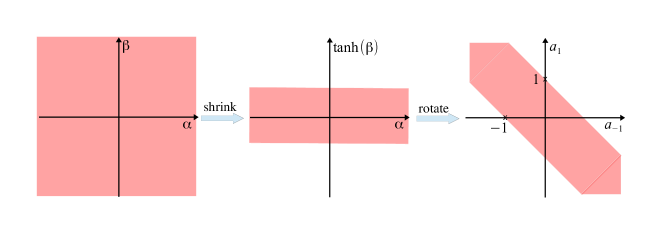
Figure 17: Visualization of the re-parameterization in Equation D.21.

References

- [1] Samy Bengio, Oriol Vinyals, Navdeep Jaitly, and Noam Shazeer. Scheduled sampling for sequence prediction with recurrent neural networks. In Advances in Neural Information Processing Systems, pages 1171–1179, 2015.
- [2] Dimitri P Bertsekas and Athena Scientific. Convex optimization algorithms. Athena Scientific Belmont, 2015.
- [3] George EP Box, Gwilym M Jenkins, Gregory C Reinsel, and Greta M Ljung. Time series analysis: forecasting and control. John Wiley & Sons, 2015.
- [4] Wonmin Byeon, Thomas M Breuel, Federico Raue, and Marcus Liwicki. Scene labeling with lstm recurrent neural networks. In Proceedings of the IEEE Conference on Computer Vision and Pattern Recognition, pages 3547–3555, 2015.
- [5] Wonmin Byeon, Qin Wang, Rupesh Kumar Srivastava, and Petros Koumoutsakos. Contextvp: Fully context-aware video prediction. In Proceedings of the European Conference on Computer Vision (ECCV), pages 753–769, 2018.
- [6] Liang-Chieh Chen, George Papandreou, Iasonas Kokkinos, Kevin Murphy, and Alan L Yuille. Deeplab: Semantic image segmentation with deep convolutional nets, atrous convolution, and fully connected crfs. IEEE transactions on pattern analysis and machine intelligence, 40(4):834–848, 2017.
- [7] Liang-Chieh Chen, George Papandreou, Florian Schroff, and Hartwig Adam. Rethinking atrous convolution for semantic image segmentation. arXiv preprint arXiv:1706.05587, 2017.
- [8] Noel CF Codella, David Gutman, M Emre Celebi, Brian Helba, Michael A Marchetti, Stephen W Dusza, Aadi Kalloo, Konstantinos Liopyris, Nabin Mishra, Harald Kittler, et al. Skin lesion analysis toward melanoma detection: A challenge at the 2017 international symposium on biomedical imaging (isbi), hosted by the international skin imaging collaboration (isic). In 2018 IEEE 15th International Symposium on Biomedical Imaging (ISBI 2018), pages 168–172. IEEE, 2018.
- [9] Jifeng Dai, Yi Li, Kaiming He, and Jian Sun. R-fcn: Object detection via region-based fully convolutional networks. In Advances in neural information processing systems, pages 379–387, 2016.
- [10] Jifeng Dai, Haozhi Qi, Yuwen Xiong, Yi Li, Guodong Zhang, Han Hu, and Yichen Wei. Deformable convolutional networks. In Proceedings of the IEEE international conference on computer vision, pages 764–773, 2017.
- [11] Github repo. https://github.com/jthsieh/DDPAE-video-prediction/blob/master/data/moving_mnist.py. [Online; accessed 05-Jan-2020].
- [12] Xavier Glorot and Yoshua Bengio. Understanding the difficulty of training deep feedforward neural networks. In Proceedings of the thirteenth international conference on artificial intelligence and statistics, pages 249–256, 2010.
- [13] Kaiming He, Xiangyu Zhang, Shaoqing Ren, and Jian Sun. Deep residual learning for image recognition. In Proceedings of the IEEE conference on computer vision and pattern recognition, pages 770–778, 2016.
- [14] Matthias Holschneider, Richard Kronland-Martinet, Jean Morlet, and Ph Tchamitchian. A real-time algorithm for signal analysis with the help of the wavelet transform. In Wavelets, pages 286–297. Springer, 1990.
- [15] Yunho Jeon and Junmo Kim. Active convolution: Learning the shape of convolution for image classification. In Proceedings of the IEEE Conference on Computer Vision and Pattern Recognition, pages 4201–4209, 2017.
- [16] Nal Kalchbrenner, Ivo Danihelka, and Alex Graves. Grid long short-term memory. arXiv preprint arXiv:1507.01526, 2015.
- [17] Diederik P Kingma and Jimmy Ba. Adam: A method for stochastic optimization. arXiv preprint arXiv:1412.6980, 2014.
- [18] Alex Krizhevsky, Ilya Sutskever, and Geoffrey E Hinton. Imagenet classification with deep convolutional neural networks. In Advances in neural information processing systems, pages 1097–1105, 2012.
- [19] Yanghao Li, Yuntao Chen, Naiyan Wang, and Zhaoxiang Zhang. Scale-aware trident networks for object detection. In Proceedings of the IEEE International Conference on Computer Vision, pages 6054–6063, 2019.
- [20] Jae S Lim. Two-dimensional signal and image processing. ph, 1990.
- [21] Sifei Liu, Shalini De Mello, Jinwei Gu, Guangyu Zhong, Ming-Hsuan Yang, and Jan Kautz. Learning affinity via spatial propagation networks. In Advances in Neural Information Processing Systems, pages 1520–1530, 2017.
- [22] Sifei Liu, Jinshan Pan, and Ming-Hsuan Yang. Learning recursive filters for low-level vision via a hybrid neural network. In European Conference on Computer Vision, pages 560–576. Springer, 2016.
- [23] Jonathan Long, Evan Shelhamer, and Trevor Darrell. Fully convolutional networks for semantic segmentation. In Proceedings of the IEEE conference on computer vision and pattern recognition, pages 3431–3440, 2015.
- [24] Wenjie Luo, Yujia Li, Raquel Urtasun, and Richard Zemel. Understanding the effective receptive field in deep convolutional neural networks. In Advances in neural information processing systems, pages 4898–4906, 2016.
- [25] Takeru Miyato, Toshiki Kataoka, Masanori Koyama, and Yuichi Yoshida. Spectral normalization for generative adversarial networks. In International Conference on Learning Representations, 2018.
- [26] Ozan Oktay, Jo Schlemper, Loic Le Folgoc, Matthew Lee, Mattias Heinrich, Kazunari Misawa, Kensaku Mori, Steven McDonagh, Nils Y Hammerla, Bernhard Kainz, et al. Attention u-net: Learning where to look for the pancreas. arXiv preprint arXiv:1804.03999, 2018.
- [27] Aaron van den Oord, Nal Kalchbrenner, and Koray Kavukcuoglu. Pixel recurrent neural networks. arXiv preprint arXiv:1601.06759, 2016.
- [28] Alan V Oppenheim, John R Buck, and Ronald W Schafer. Discrete-time signal processing. 2014.
- [29] Olaf Ronneberger, Philipp Fischer, and Thomas Brox. U-net: Convolutional networks for biomedical image segmentation. In International Conference on Medical image computing and computer-assisted intervention, pages 234–241. Springer, 2015.
- [30] Karen Simonyan and Andrew Zisserman. Very deep convolutional networks for large-scale image recognition. arXiv preprint arXiv:1409.1556, 2014.
- [31] Marijn F Stollenga, Wonmin Byeon, Marcus Liwicki, and Juergen Schmidhuber. Parallel multi-dimensional lstm, with application to fast biomedical volumetric image segmentation. In Advances in neural information processing systems, pages 2998–3006, 2015.
- [32] Ashish Vaswani, Noam Shazeer, Niki Parmar, Jakob Uszkoreit, Llion Jones, Aidan N Gomez, Łukasz Kaiser, and Illia Polosukhin. Attention is all you need. In Advances in neural information processing systems, pages 5998–6008, 2017.
- [33] Xiaolong Wang, Ross Girshick, Abhinav Gupta, and Kaiming He. Non-local neural networks. In Proceedings of the IEEE conference on computer vision and pattern recognition, pages 7794–7803, 2018.
- [34] Zhengyang Wang and Shuiwang Ji. Smoothed dilated convolutions for improved dense prediction. In Proceedings of the 24th ACM SIGKDD International Conference on Knowledge Discovery & Data Mining, pages 2486–2495, 2018.
- [35] Zhengyang Wang, Na Zou, Dinggang Shen, and Shuiwang Ji. Non-local u-nets for biomedical image segmentation. In AAAI, pages 6315–6322, 2020.
- [36] Zhou Wang, Alan C Bovik, Hamid R Sheikh, Eero P Simoncelli, et al. Image quality assessment: from error visibility to structural similarity. IEEE transactions on image processing, 13(4):600–612, 2004.
- [37] Webpage. https://challenge2018.isic-archive.com. [Online; accessed 29-May-2020].
- [38] SHI Xingjian, Zhourong Chen, Hao Wang, Dit-Yan Yeung, Wai-Kin Wong, and Wang-chun Woo. Convolutional lstm network: A machine learning approach for precipitation nowcasting. In Advances in neural information processing systems, pages 802–810, 2015.
- [39] Fisher Yu and Vladlen Koltun. Multi-scale context aggregation by dilated convolutions. arXiv preprint arXiv:1511.07122, 2015.
- [40] Fisher Yu, Vladlen Koltun, and Thomas Funkhouser. Dilated residual networks. In Proceedings of the IEEE conference on computer vision and pattern recognition, pages 472–480, 2017.
- [41] Xizhou Zhu, Han Hu, Stephen Lin, and Jifeng Dai. Deformable convnets v2: More deformable, better results. In Proceedings of the IEEE Conference on Computer Vision and Pattern Recognition, pages 9308–9316, 2019.