Query-Efficient Correlation Clustering

Abstract.

Correlation clustering is arguably the most natural formulation of clustering. Given $n$ objects and a pairwise similarity measure, the goal is to cluster the objects so that, to the best possible extent, similar objects are put in the same cluster and dissimilar objects are put in different clusters.

A main drawback of correlation clustering is that it requires as input the $\Theta(n^{2})$ pairwise similarities. This is often infeasible to compute or even just to store. In this paper we study query-efficient algorithms for correlation clustering. Specifically, we devise a correlation clustering algorithm that, given a budget of $Q$ queries, attains a solution whose expected number of disagreements is at most $3\cdot\operatorname{OPT}+O(\frac{n^{3}}{Q})$, where $\operatorname{OPT}$ is the optimal cost for the instance. Its running time is $O(Q)$, and can be easily made non-adaptive (meaning it can specify all its queries at the outset and make them in parallel) with the same guarantees. Up to constant factors, our algorithm yields a provably optimal trade-off between the number of queries $Q$ and the worst-case error attained, even for adaptive algorithms.

Finally, we perform an experimental study of our proposed method on both synthetic and real data, showing the scalability and the accuracy of our algorithm.

1. Introduction

Correlation clustering (Bansal et al., 2004) (or cluster editing) is a prominent clustering framework where we are given a set $V=[n]$ and a symmetric pairwise similarity function $\operatorname{sim}:\binom{V}{2}\rightarrow\{0,1\}$, where $\binom{V}{2}$ is the set of unordered pairs of elements of $V$. The goal is to cluster the items in such a way that, to the best possible extent, similar objects are put in the same cluster and dissimilar objects are put in different clusters. Assuming that cluster identifiers are represented by natural numbers, a clustering $\operatorname{\ell}$ is a function $\operatorname{\ell}:V\rightarrow\mathbb{N}$, and each cluster is a maximal set of vertices sharing the same label. Correlation clustering aims at minimizing the following cost:

(1) $$\operatorname{cost}(\operatorname{\ell})=\sum_{\begin{subarray}{c}(x,y)\in\binom{V}{2},\\ \operatorname{\ell}(x)=\operatorname{\ell}(y)\end{subarray}}(1-\operatorname{sim}(x,y))\mspace{5.0mu}+\mspace{-15.0mu}\sum_{\begin{subarray}{c}(x,y)\in\binom{V}{2},\\ \operatorname{\ell}(x)\not=\operatorname{\ell}(y)\end{subarray}}\operatorname{sim}(x,y).$$

The intuition underlying the above problem definition is that if two objects $x$ and $y$ are dissimilar and are assigned to the same cluster we should pay a cost of $1$, i.e., the amount of their dissimilarity. Similarly, if $x,y$ are similar and they are assigned to different clusters we should pay also cost $1$, i.e., the amount of their similarity $\operatorname{sim}(x,y)$. The correlation clustering framework naturally extends to non-binary, symmetric function, i.e., $\operatorname{sim}:\binom{V}{2}\rightarrow[0,1]$. In this paper we focus on the binary case; the general non-binary case can be efficiently reduced to this case at a loss of only a constant factor in the approximation (Bansal et al., 2004, Thm. 23). The binary setting can be viewed very conveniently through graph-theoretic lenses: the $n$ items correspond to the vertices of a similarity graph $G$, which is a complete undirected graph with edges labeled “+” or “-”. An edge $e$ causes a disagreement (of cost 1) between the similarity graph and a clustering when it is a “+” edge connecting vertices in different clusters, or a “–” edge connecting vertices within the same cluster. If we were given a cluster graph (Shamir et al., 2004), i.e., a graph whose set of positive edges is the union of vertex-disjoint cliques, we would be able to produce a perfect (i.e., cost 0) clustering simply by computing the connected components of the positive graph. However, similarities will generally be inconsistent with one another, so incurring a certain cost is unavoidable. Correlation clustering aims at minimizing such cost. The problem may be viewed as the task of finding the equivalence relation that most closely resembles a given symmetric relation. The correlation clustering problem is NP-hard (Bansal et al., 2004; Shamir et al., 2004).

Correlation clustering is particularly appealing for the task of clustering structured objects, where the similarity function is domain-specific. A typical application is clustering web-pages based on similarity scores: for each pair of pages we have a score between 0 and 1, and we would like to cluster the pages so that pages with a high similarity score are in the same cluster, and pages with a low similarity score are in different clusters. The technique is applicable to a multitude of problems in different domains, including duplicate detection and similarity joins (Hassanzadeh et al., 2009; Demaine et al., 2006), spam detection (Ramachandran et al., 2007; Bonchi et al., 2014), co-reference resolution (McCallum and Wellner, 2005), biology (Ben-Dor et al., 1999; Bonchi et al., 2013b), image segmentation (Kim et al., 2011), social networks (Bonchi et al., 2015), and clustering aggregation (Gionis et al., 2007). A key feature of correlation clustering is that it does not require the number of clusters as part of the input; instead it automatically finds the optimal number, performing model selection.

Despite its appeal, the main practical drawback of correlation clustering is the fact that, given $n$ items to be clustered, $\Theta(n^{2})$ similarity computations are needed to prepare the similarity graph that serves as input for the algorithm. In addition to the obvious algorithmic cost involved with $\Theta(n^{2})$ queries, in certain applications there is an additional type of cost that may render correlation clustering algorithms impractical. Consider the following motivating real-world scenarios. In biological sciences, in order to produce a network of interactions between a set of biological entities (e.g., proteins), a highly trained professional has to devote time and costly resources (e.g., equipment) to perform tests between all ${n\choose 2}$ pairs of entities. In entity resolution, a task central to data integration and data cleaning (Wang et al., 2012), a crowdsourcing-based approach performs queries to workers of the form “does the record $x$ represent the same entity as the record $y$?”. Such queries to workers involve a monetary cost, so it is desirable to reduce their number. In both scenarios developing clustering tools that use fewer than ${n\choose 2}$ queries is of major interest. This is the main motivation behind our work. At a high level we answer the following question:

Problem 1.

How to design a correlation clustering algorithm that outputs a good approximation in a query-efficient manner: i.e., given a budget of $Q$ queries, the algorithm is allowed to learn the specific value of $\operatorname{sim}(i,j)\in\{0,1\}$ for up to $Q$ queries $(i,j)$ of the algorithm’s choice.

Contributions. The main contributions of this work are summarized as follows:

• We design a computationally efficient randomized algorithm QECC that, given a budget of $Q$ queries, attains a solution whose expected number of disagreements is at most $3\cdot\operatorname{OPT}+O(\frac{n^{3}}{Q})$, where $\operatorname{OPT}$ is the optimal cost of the correlation clustering instance (Theorem LABEL:thm:ub). We can achieve this via a non-adaptive algorithm (Theorem LABEL:thm:ub2).

• We show (Theorem LABEL:thm:lb) that up to constant factors, our algorithm is optimal, even for adaptive algorithms: any algorithm making $Q$ queries must make at least $\Omega(\operatorname{OPT}+\frac{n^{3}}{Q})$ errors.

• We give a simple, intuitive heuristic modification of our algorithm QECC-heur which helps reduce the error of the algorithm in practice (specifically the recall of positive edges), thus partially bridging the constant-factor gap between our lower and upper bounds.

• We present an experimental study of our two algorithms, compare their performance with a baseline based on affinity propagation, and study their sensitivity to parameters such as graph size, number of clusters, imbalance, and noise.

2. Related work

We review briefly the related work that lies closest to our paper.

Correlation clustering. The correlation clustering problem is NP-hard (Bansal et al., 2004; Shamir et al., 2004) and, in its minimizing disagreements formulation used above, is also APX-hard (Charikar et al., 2005), so we do not expect a polynomial-time approximation scheme. Nevertheless, there are constant-factor approximation algorithms (Bansal et al., 2004; Charikar et al., 2005; Ailon et al., 2008). Ailon et al. (Ailon et al., 2008) present QwickCluster, a simple, elegant 3-approximation algorithm. They improve the approximation ratio to $2.5$ by utilizing an LP relaxation of the problem; the best approximation factor known to date is $2.06$, due to Chawla et al. (Chawla et al., 2015). The interested reader may refer to the extensive survey due to Bonchi, García-Soriano and Liberty (Bonchi et al., 2014).

Query-efficient algorithms for correlation clustering. Query-efficient correlation clustering has received less attention. There exist two categories of algorithms, non-adaptive and adaptive. The former choose their queries before-hand, while the latter can select the next query based on the response to previous queries.

In an earlier preprint (Bonchi et al., 2013a) we initiated the study of query-efficient correlation clustering. Our work there focused on a stronger local model which requires answering cluster-id queries quickly, i.e., outputting a cluster label for each given vertex by querying at most $q$ edges per vertex. Such a $q$-query local algorithm allows a global clustering of the graph with $qn$ queries; hence upper bounds for local clustering imply upper bounds for global clustering, which is the model we consider in this paper. The algorithm from (Bonchi et al., 2013a) is non-adaptive, and the upper bounds we present here (Theorems LABEL:thm:ub and LABEL:thm:ub2) may be recovered by setting $\epsilon=\frac{n}{Q}$ in (Bonchi et al., 2013a, Thm. 3.3). A matching lower bound was also proved in (Bonchi et al., 2013a, Thm. 6.1), but the proof therein applied only to non-adaptive algorithms. In this paper we present a self-contained analysis of the algorithm from (Bonchi et al., 2013a) in the global setting (Theorems LABEL:thm:ub and LABEL:thm:ub2) and strengthen the lower bound so that it applies also to adaptive algorithms (Theorem LABEL:thm:lb). Additionally, we perform an experimental study of the algorithm.

Some of the results from (Bonchi et al., 2013a) have been rediscovered several years later (in a weaker form) by Bressan, Cesa-Bianchi, Paudice, and Vitale (Bressan et al., 2019). They study the problem of query-efficient correlation clustering (Problem 1) in the adaptive setting, and provide a query-efficient algorithm, named ACC. The performance guarantee they obtain in (Bressan et al., 2019, Thm. 1) is asymptotically the same that had already been proven in (Bonchi et al., 2013a), but it has worse constant factors and is attained via an adaptive algorithm. They also modify the lower bound proof from (Bonchi et al., 2013a) to make it adaptive (Bressan et al., 2019, Thm. 9), and present some new results concerning the cluster-recovery properties of the algorithm.

In terms of techniques, the only difference between our algorithm QECC and the ACC algorithm from (Bressan et al., 2019) is that the latter adds a check that discards pivots when no neighbor is found after inspecting a random sample of size $f(n-1)=Q/(n-1)$. This additional check is unnecessary from a theoretical viewpoint (see Theorem LABEL:thm:ub) and it has the disadvantage that it necessarily results in an adaptive algorithm. Moreover, the analysis of  (Bressan et al., 2019) is significantly more complex than ours, because they need to adapt the proof of the approximation guarantees of the QwickCluster algorithm from  (Ailon et al., 2008) to take into account the additional check, whereas we simply take the approximation guarantee as given and argue that stopping QwickCluster after $k$ pivots have been selected only incurs an expected additional cost of $n^{2}/(2k)$ (Lemma LABEL:lem:indep).

3. Algorithm and analysis

Before presenting our algorithm, we describe in greater detail the elegant algorithm due to Ailon et al. (Ailon et al., 2008) for correlation clustering, as it lies close to our proposed method.

QwickCluster algorithm. The QwickCluster algorithm selects a random pivot $v$, creates a cluster with $v$ and its positive neighborhood, removes the cluster, and iterates on the induced remaining subgraph. Essentially it finds a maximal independent set in the positive graph in random order. The elements in this set serve as cluster centers (pivots) in the order in which they were found. In the pseudocode below, $\Gamma_{G}^{+}(v)$ denotes the set of vertices to which there is a positive edge in $G$ from $v$.

$G=(V,E)$, a complete graph with “+,-” edge labels

$R\leftarrow V$ $\triangleright$ Unclustered vertices so far

while $R\neq\emptyset$ do

     Pick a pivot $v$ from $R$ uniformly at random.

     Output cluster $C=\{v\}\cup\Gamma_{G}^{+}(v)\cap R$.

     $R\leftarrow V\setminus C$

Algorithm 1 QwickCluster

When the graph is clusterable, QwickCluster makes no mistakes. In (Ailon et al., 2008), the authors show that the expected cost of the clustering found by QwickCluster is at most $3\operatorname{OPT}$, where $\operatorname{OPT}$ denotes the optimal cost.

QECC. Our algorithm QECC (Query-Efficient Correlation Clustering) runs QwickCluster until the query budget $Q$ is complete, and then outputs singleton clusters for the remaining unclustered vertices.

$G=(V,E)$; query budget $Q$

$R\leftarrow V$ $\triangleright$ Unclustered vertices so far

while $R\neq\emptyset\wedge Q\geq|R|-1$ do

     Pick a pivot $v$ from $R$ uniformly at random.

     Query all pairs $(v,w)$ for $w\in R\setminus\{v\}$ to determine $\Gamma_{G}^{+}(v)\cap R$.

     $Q\leftarrow Q-|R|+1$

     Output cluster $C=\{v\}\cup\Gamma_{G}^{+}(v)\cap R$.

     $R\leftarrow V\setminus C$

Output a separate singleton cluster for each remaining $v\in R$.

Algorithm 2 QECC

The following subsection is devoted to the proof of our main result, stated next.

Theorem 3.1.

Let $G$ be a graph with $n$ vertices. For any $Q>0$, Algorithm QECC finds a clustering of $G$ with expected cost at most $3\cdot\operatorname{OPT}+\frac{n^{3}}{2Q}$ making at most $Q$ edge queries. It runs in time $O(Q)$ assuming unit-cost queries.

3.1. Analysis of QECC

For simplicity, in the rest of this section we will identify a complete “+,-” labeled graph $G$ with its graph of positive edges $(V,E^{+})$, so that queries correspond to querying a pair of vertices for the existence of an edge. The set of (positive) neighbors of $v$ in a graph $G=(V,E)$ will be denoted $\Gamma(v)$; a similar notation is used for the set $\Gamma(S)$ of positive neighbors of a set $S\subseteq V$. The cost of the optimum clustering for $G$ is denoted $\operatorname{OPT}$. When $\ell$ is a clustering, $\operatorname{cost}(\ell)$ denotes the cost (number of disagreements) of this clustering, defined by (LABEL:equation:correlation-clustering) with $\operatorname{sim}(x,y)=1$ iff $\{x,y\}\in E$.

In order to analyze QECC, we need to understand how early stopping of QwickCluster affects the accuracy of the clustering found. For any non-empty graph $G$ and pivot $v\in V(G)$, let $N_{v}(G)$ denote the subgraph of $G$ resulting from removing all edges incident to $\Gamma(v)$ (keeping all vertices). Define a random sequence $G_{0},G_{1},\ldots$ of graphs by $G_{0}=G$ and $G_{i+1}=N_{v_{i+1}}(G_{i})$, where $v_{1},v_{2},\ldots$ are chosen independently and uniformly at random from $V(G_{0})$. Note that $G_{i+1}=G_{i}$ if at step $i$ a vertex is chosen for a second time.

The following lemma is key:

Lemma 3.2.

Let $G_{i}$ have average degree $\tilde{d}$. When going from $G_{i}$ to $G_{i+1}$, the number of edges decreases in expectation by at least $\binom{\tilde{d}+1}{2}$.

Proof.

Let $V=V(G_{0})$, $E=E(G_{i})$ and let $d_{u}=|\Gamma(u)|$ denote the degree of $u\in V$ in $G_{i}$. Consider an edge $\{u,v\}\in E$. It is deleted if the chosen pivot $v_{i}$ is an element of $\Gamma(u)\cup\Gamma(v)$ (which contains $u$ and $v$). Let $X_{uv}$ be the 0-1 random variable associated with this event, which occurs with probability

$$\operatorname*{\mathbb{E}}[X_{uv}]=\frac{|\Gamma(u)\cup\Gamma(v)|}{n}\geq\frac{1+\max(d_{u},d_{v})}{n}\geq\frac{1}{n}+\frac{d_{u}+d_{v}}{2n}.$$

Let $D=\sum_{u<v\mid{\{u,v\}}\in E}X_{uv}$ be the number of edges deleted (we assume an ordering of $V$ to avoid double-counting edges). By linearity of expectation,

$$\operatorname*{\mathbb{E}}[D] = \sum_{\begin{subarray}{c}u<v\\ \{u,v\}\in E\end{subarray}}\operatorname*{\mathbb{E}}[X_{uv}]=\frac{1}{2}\sum_{\begin{subarray}{c}u,v\in V\\ \{u,v\}\in E\end{subarray}}\operatorname*{\mathbb{E}}[X_{uv}]$$

$$\geq \frac{1}{2}\sum_{\begin{subarray}{c}u,v\\ \{u,v\}\in E\end{subarray}}\left(\frac{1}{n}+\frac{d_{u}+d_{v}}{2n}\right)$$

$$= \frac{\tilde{d}}{2}+\frac{1}{4n}\sum_{\begin{subarray}{c}u,v\\ \{u,v\}\in E\end{subarray}}(d_{u}+d_{v}).$$

Now we compute

$$\frac{1}{4n}\sum_{\begin{subarray}{c}u,v\\ \{u,v\}\in E\end{subarray}}(d_{u}+d_{v}) = \frac{1}{2n}\sum_{\begin{subarray}{c}u,v\\ \{u,v\}\in E\end{subarray}}d_{u}=\frac{1}{2n}\sum_{u}d_{u}^{2}$$

$$= \frac{1}{2}\operatorname*{\mathbb{E}}_{u\sim V}[d_{u}^{2}]\geq\frac{1}{2}\left(\operatorname*{\mathbb{E}}_{u\sim V}[d_{u}]\right)^{2}=\frac{1}{2}\tilde{d}^{2},$$

where in the last line, $\sim$ denotes uniform sampling and we used the Cauchy-Schwarz inequality. Hence $\operatorname*{\mathbb{E}}[D]\geq\frac{\tilde{d}}{2}+\frac{\tilde{d}^{2}}{2}=\binom{\tilde{d}+1}{2}.$ ∎

Lemma 3.3.

Let $G$ be a graph with $n$ vertices and let $P=\{v_{1},\ldots,v_{r}\}$ be the first $r$ pivots chosen by running QwickCluster on $G$. Then the expected number of positive edges of $G$ not incident with an element of $P\cup\Gamma(P)$ is less than $\frac{n^{2}}{2(r+1)}$.

Proof.

Recall that at each iteration QwickCluster picks a random pivot from $R$. This selection is equivalent to picking a random pivot $v$ from the original set of vertices $V$ and discarding it if $v\notin R$, repeating until some $v\in R$ is found, in which case a new pivot is added. Consider the following modification of QwickCluster, denoted SluggishCluster, which picks a pivot $v$ at random from $V$ but always increases the counter $r$ of pivots found, even if $v\in R$ (ignoring the cluster creation step if $v\notin R$). We can couple both algorithms into a common probability space where each point $\omega$ contains a sequence of randomly selected vertices and each algorithm picks the next one in sequence. For any $\omega$, whenever the first $r$ pivots of SluggishCluster are $S=(v_{1},\ldots,v_{r})$, then the first $r^{\prime}$ pivots of QwickCluster are the sequence $S^{\prime}$ obtained from $S$ by removing previously appearing elements, where $r^{\prime}=|S^{\prime}|$. Hence $|V\setminus(S\cup\Gamma(S))|=|V\setminus(S^{\prime}\cup\Gamma(S^{\prime}))|$ and $r^{\prime}\leq r$. Thus the number of edges not incident with the first $r$ pivots and their neighbors in SluggishCluster stochastically dominates the number of edges not incident with the first $r$ pivots and their neighbors in SluggishCluster, since both numbers are decreasing with $r$.

Therefore it is enough to prove the claim for SluggishCluster. Let $n=|V(G_{0})|$ and define $\alpha_{i}\in[0,1]$ by $\alpha_{i}=\frac{2\cdot|E(G_{i})|}{n^{2}}.$ We claim that for all $i\geq 1$ the following inequalities hold:

(2) $$\operatorname*{\mathbb{E}}[\alpha_{i}\mid G_{0},\ldots,G_{i-1}] \leq\alpha_{i-1}(1-\alpha_{i-1}),$$

(3) $$\operatorname*{\mathbb{E}}[\alpha_{i}] \leq\operatorname*{\mathbb{E}}[\alpha_{i-1}](1-\operatorname*{\mathbb{E}}[\alpha_{i-1}]),$$

(4) $$\operatorname*{\mathbb{E}}[\alpha_{i}] <\frac{1}{i+1}.$$

Indeed, $G_{i}$ is a random function of $G_{i-1}$ only, and the average degree of $G_{i-1}$ is $\widetilde{d}_{i-1}=\alpha_{i-1}n$ so, by Lemma LABEL:lem:del_edges,

$$\operatorname*{\mathbb{E}}[2\cdot|E(G_{i})|\mid G_{i-1}]\leq\alpha_{i-1}n^{2}-2\cdot\frac{1}{2}\widetilde{d}_{i-1}^{2}=n^{2}\alpha_{i-1}(1-\alpha_{i-1}),$$

proving (LABEL:eq:cond_alpha_i). Now (LABEL:eq:alpha_i) now follows from Jensen’s inequality: since

$$\operatorname*{\mathbb{E}}[\alpha_{i}]=\operatorname*{\mathbb{E}}\big{[}\operatorname*{\mathbb{E}}[\alpha_{i}\mid G_{0},\ldots,G_{i-1}]\big{]}\leq\operatorname*{\mathbb{E}}[\alpha_{i-1}(1-\alpha_{i-1})]$$

and the function $g(x)=x(1-x)$ is concave in $[0,1]$, we have

$$\operatorname*{\mathbb{E}}[\alpha_{i}]\leq\operatorname*{\mathbb{E}}[g(\alpha_{i-1})]\leq g(\operatorname*{\mathbb{E}}[\alpha_{i-1}])=\operatorname*{\mathbb{E}}[\alpha_{i-1}](1-\operatorname*{\mathbb{E}}[\alpha_{i-1}]).$$

Finally we prove $\operatorname*{\mathbb{E}}[\alpha_{i}]<1/(i+1)\;\forall i\geq 1$. For $i=1$, we have:

$$\operatorname*{\mathbb{E}}[\alpha_{1}]\leq g(\alpha_{0})\leq\max_{x\in[0,1]}g(x)=g\left(\frac{1}{2}\right)=\frac{1}{4}<\frac{1}{2}.$$

For $i>1$, observe that $g$ is increasing on $[0,1/2]$ and

$$g\left(\frac{1}{i}\right)=\frac{1}{i}-\frac{1}{i^{2}}\leq\frac{1}{i}-\frac{1}{i(i+1)}=\frac{1}{i+1},$$

so (LABEL:eq:alpha_i2) follows from (LABEL:eq:alpha_i) by induction on $i$:

$$\operatorname*{\mathbb{E}}[\alpha_{i-1}]<\frac{1}{i}\implies\operatorname*{\mathbb{E}}[\alpha_{i}]\leq g\left(\frac{1}{i}\right)\leq\frac{1}{i+1}.$$

Therefore $\operatorname*{\mathbb{E}}[|E(G_{r})|]=\frac{1}{2}\operatorname*{\mathbb{E}}[\alpha_{r}]n^{2}\leq\frac{n^{2}}{2(r+1)}$, as we wished to show. ∎

We are now ready to prove Theorem LABEL:thm:ub:

Proof of Theorem LABEL:thm:ub.  Let $\operatorname{OPT}$ denote the cost of the optimal clustering of $G$ and let $C_{r}$ be a random variable denoting the clustering obtained by stopping QwickCluster after $r$ pivots are found (or running it to completion if it finds $r$ pivots or less), and putting all unclustered vertices into singleton clusters. Note that whenever $C_{i}$ makes a mistake on a negative edge, so does $C_{j}$ for $j\geq i$; on the other hand, every mistake on a positive edge by $C_{i}$ is either a mistake by $C_{j}$ ($j\geq i$) or the edge is not incident to any of the vertices clustered in the first $i$ rounds. By Lemma LABEL:lem:indep, there are at most $\frac{n^{2}}{2(i+1)}$ of the latter in expectation. Hence $\operatorname*{\mathbb{E}}[\operatorname{cost}(C_{i})]-\operatorname*{\mathbb{E}}[\operatorname{cost}(C_{n})]\leq\frac{n^{2}}{2(i+1)}$.

Algorithm QECC runs for $k$ rounds, where $k\geq\lfloor\frac{Q}{n-1}\rfloor>\frac{Q}{n}-1$ because each pivot uses $|R|-1\leq n-1$ queries. Then

$$\operatorname*{\mathbb{E}}[\operatorname{cost}(C_{k})]-\operatorname*{\mathbb{E}}[\operatorname{cost}(C_{n})]<\frac{n^{2}}{2(k+1)}<\frac{n^{3}}{2Q}.$$

On the other hand, we have $\operatorname*{\mathbb{E}}[\operatorname{cost}(C_{n})]\leq 3\cdot\operatorname{OPT}$ because of the expected 3-approximation guarantee of QwickCluster from (Ailon et al., 2008). Thus $\operatorname*{\mathbb{E}}[\operatorname{cost}(C_{k})]\leq 3\operatorname{OPT}+\frac{n^{3}}{2Q}$, proving our approximation guarantee.

Finally, the time spent inside each iteration of the main loop is dominated by the time spent making queries to vertices in $R$, since this number also bounds the size of the cluster found. Therefore the running time of QECC is $O(Q)$. ∎

3.2. A non-adaptive algorithm.

Our algorithm QECC is adaptive in the way we have chosen to present it: the queries made when picking a second pivot depend on the result of the queries made for the first pivot. However, this is not necessary: we can instead query for the neighborhood of a random sample $S$ of size $\frac{Q}{n-1}$. If we use the elements of $S$ to find pivots, the same analysis shows that the output of this variant meets the exact same error bound of $3\operatorname{OPT}+n^{3}/(2Q)$. For completeness, we include pseudocode for the adaptive variant of QECC below (Algorithm 3).

In practice the adaptive variant we have presented in Algorithm 2 will run closer to the query budget, choosing more pivots and reducing the error somewhat below the theoretical bound, because it does not “waste” queries between a newly found pivot and the neighbors of previous pivots. Nevertheless, in settings where the similarity computations can be performed in parallel, it may become advantageous to use Non-adaptive QECC. Another benefit of the non-adaptive variant is that it gives a one-pass streaming algorithm for correlation clustering that uses only $O(Q)$ space and processes edges in arbitrary order.

Theorem 3.4.

For any $Q>0$, Algorithm Non-adaptive QECC finds a clustering of $G$ with expected cost at most $3\cdot\operatorname{OPT}+\frac{n^{3}}{2Q}$ making at most $Q$ non-adaptive edge queries. It runs in time $O(Q)$ assuming unit-cost queries.

Proof.

The number of queries it makes is $S=(n-1)+(n-2)+\ldots(n-k)=\frac{2n-1-k}{2}k\leq Q.$ Note that $\frac{n-1}{2}k\leq S\leq Q\leq(n-1)k$. The proof of the error bound proceeds exactly as in the proof of Theorem LABEL:thm:ub (because $k\geq\frac{Q}{n-1}$). The running time of the querying phase of Non-adaptive QECC is $O(Q)$ and, assuming a hash table is used to store query answers, the expected running time of the second phase is bounded by $O(nk)=O(Q)$, because $k\leq\frac{2Q}{n-1}$. ∎

Another interesting consequence of this result (coupled with our lower bound, Theorem LABEL:thm:lb), is that adaptivity does not help for correlation clustering (beyond possibly a constant factor), in stark contrast to other problems where an exponential separation is known between the query complexity of adaptive and non-adaptive algorithms (e.g., (Fischer, 2004; Brody et al., 2011)).

$G=(V,E)$; query budget $Q$

$k\leftarrow\max\{t\leq n\mid(2n-1-t)t\leq 2Q\}.$

Let $S=(s_{1},\ldots,s_{k})$ be a uniform random sample from $V$

 (with or without replacement)

$\triangleright$ Querying phase: find $\Gamma_{G}^{+}(v)$ for each $v\in S$

for  each $v\in S$, $w\in V$, $v<w$  do

     Query $(v,w)$

$\triangleright$ Clustering phase

$R\leftarrow V$

$i\leftarrow 1$

while $R\neq\emptyset\wedge i\leq k$ do

     if $s_{i}\in R$ then

         Output cluster $C=\{s_{i}\}\cup\Gamma_{G}^{+}(s_{i})\cap R$.

         $R\leftarrow V\setminus C$      

     $i\leftarrow i+1$

Output a separate singleton cluster for each remaining $v\in R$.

Algorithm 3 Non-adaptive QECC

4. Lower bound

In this section we show that QECC is essentially optimal: for any given budget of queries, no algorithm (adaptive or not) can find a solution better than that of QECC by more than a constant factor.

Theorem 4.1.

For any $c\geq 1$ and $T$ such that $8n<T\leq\frac{n^{2}}{2048c^{2}}$, any algorithm finding a clustering with expected cost at most $c\cdot\operatorname{OPT}+T$ must make at least $\Omega(\frac{n^{3}}{Tc^{2}})$ adaptive edge similarity queries.

Note that this also implies that any purely multiplicative approximation guarantee needs $\Omega(n^{2})$ queries (e.g. by taking $T=10n$).

Proof.

Let $\epsilon=\frac{T}{n^{2}}$; then $\frac{1}{n}<\epsilon\leq\frac{1}{2048c^{2}}$. By Yao’s minimax principle (Yao, 1977), it suffices to produce a distribution ${\mathcal{G}}$ over graphs with the following properties:

• the expected cost of the optimal clustering of $G\sim{\mathcal{G}}$ is $\operatorname*{\mathbb{E}}[\operatorname{OPT}(G)]\leq\frac{\varepsilon n^{2}}{c};$

• for any deterministic algorithm making fewer than $L/2=\frac{n}{2048\varepsilon c^{2}}$ queries, the expected cost (over ${\mathcal{G}}$) of the clustering produced exceeds $2\varepsilon n^{2}\geq c\cdot\operatorname*{\mathbb{E}}[\operatorname{OPT}(G)]+T$.

Let $\alpha=\frac{1}{4c}$ and $k=\frac{1}{32c\varepsilon}$. We can assume that $c$, $k$ and $\alpha n/k$ are integral (here we use the fact that $\varepsilon>1/n$). Let $A=\{1,\ldots,(1-\alpha)n\}$ and $B=\{(1-\alpha)n+1,\ldots,n\}$.

Consider the following distribution ${\mathcal{G}}$ of graphs: partition the vertices of $A$ into exactly $k$ equal-sized clusters $C_{1},\ldots,C_{k}$. The set of positive edges will be the union of the cliques defined by $C_{1},\ldots,C_{k}$, plus edges joining each vertex $v\in B$ to all the elements of $C_{r_{v}}$ for a randomly chosen $r_{v}\in[k]$; $r_{v}$ is chosen independently of $r_{w}$ for all $w\neq v$.

Define the natural clustering of a graph $G\in{\mathcal{G}}$ by the classes $C_{i}^{\prime}=C_{i}\cup\{v\in B\mid r_{v}=i\}$ ($i\in[k]$). We view $N$ also as a graph formed by a disjoint union of the $k$ cliques determined by $\{C^{\prime}_{i}\}_{i\in[k]}$. This clustering will have a few disagreements because of the negative edges between different vertices $v,w\in B$ with $r_{v}=r_{w}$. For any pair of distinct elements $v,w\in B$, this happens with probability $1/k$. The cost of the optimal clustering of $G$ is bounded by that of the natural clustering $N$, hence

$$\operatorname*{\mathbb{E}}[\operatorname{OPT}]\leq\operatorname*{\mathbb{E}}[\operatorname{cost}(N)]=\frac{\binom{\alpha n}{2}}{k}\leq\frac{\alpha^{2}n^{2}}{2k}=\frac{\varepsilon}{c}n^{2}.$$

We have to show that any algorithm making $<L/2$ queries to graphs drawn from ${\mathcal{G}}$ produces a clustering with expected cost larger than $2\varepsilon n^{2}$. Since all graphs in ${\mathcal{G}}$ induce the same subgraphs on $A$ and $B$ separately, we can assume without loss of generality that the algorithm queries only edges between $A$ and $B$. Note that the neighborhoods in $G$ of every pair of vertices from the same $C_{i}$ are the same: $\Gamma^{+}_{G}(u)=\Gamma^{+}_{G}(v)$ and $\Gamma^{-}_{G}(u)=\Gamma^{-}_{G}(v)$ for all $u,v\in C_{i}$, $i\in[k]$; moreover, $u$ and $v$ are joined by a positive edge. Therefore, if $u,v\in C_{i}$ but the algorithm assigns $u$ and $v$ to different clusters, either moving $u$ to $v$’s cluster or $v$ to $u$’s cluster will not decrease the cost. All in all, we can assume that the algorithm outputs $k$ clusters $C^{\prime}_{1},\ldots,C^{\prime}_{k}$ with $C_{i}\subseteq C^{\prime}_{i}$ for all $i$, plus (possibly) some clusters $C^{\prime}_{k+1},\ldots,C^{\prime}_{k^{\prime}}$ ($k^{\prime}\geq k$) involving only elements of $B$.

For $v\in B$, let $s_{v}\in[k^{\prime}]$ denote the cluster that the algorithm assigns $v$ to. For every $v\in B$, let $G_{v}$ denote the event that the algorithm queries $(u,v)$ for some $u\in C_{r_{v}}$ and, whenever $G_{v}$ does not hold, let us add a “fictitious” query to the algorithm between $v$ and some arbitrary element of $C_{s_{v}}$. This ensures that whenever $r_{v}=s_{v}$, the last query of the algorithm verifies its guess and returns 1 if the correct cluster has been found. This adds at most $|B|\leq n\leq\frac{L}{2}$ queries in total. Let $Q_{1},Q_{2},\ldots,Q_{z}$ be the (random) sequence of queries issued by the algorithm and let $i^{v}_{1},i^{v}_{2},\ldots,i^{v}_{T_{v}}$ be the indices of those queries involving a fixed vertex $v\in B$. Note that $r_{v}$ is independent of the response to all queries not involving $v$ and, conditioned on the result of all queries up to time $t<i_{T_{v}}$, $r_{v}$ is uniformly distributed among the set $\{i\in[k]\mid(Q_{j}\notin C_{i}\forall j<t)\}$, whose size is upper-bounded by $k-t+1$. Therefore

$$\Pr[Q_{i^{v}_{t}}\in C_{r_{v}}\mid Q_{1},\ldots,Q_{i^{v}_{t-1}}]\leq\frac{1}{k-t+1},$$

which becomes an equality if the algorithm does not query the same cluster twice. It follows by induction that

(5) $$\Pr[\{Q_{i^{v}_{1}},\ldots,Q_{i^{v}_{t}}\}\cap C_{r_{v}}\neq\emptyset]\leq\frac{t}{k}.$$

Let $M_{v}$ be the event that the algorithm makes more than $k/2$ queries involving $v$. The event $r_{v}=s_{v}$ is equivalent to $G_{v}$, i.e., the event $\{Q_{i^{v}_{1}},\ldots,Q_{i^{v}_{T^{v}}}\}\cap C_{r_{v}}\neq\emptyset$, because of our addition of one fictitious query for $v$. We have

$$\Pr[r_{v}=s_{v}]=\Pr[G_{v}]\leq\Pr[M_{v}]+\Pr[G_{v}\wedge\overline{M}_{v}].$$

In other words, either the algorithm makes many queries for $v$, or it hits the correct cluster with few queries. (Without fictitious queries, we would have to add a third term for the probability that the algorithm picks by chance the correct $s_{v}$.) We will use the first term $\Pr[M_{v}]$ to control the expected query complexity. The second term, $\Pr[G_{v}\wedge\overline{M}_{v}]$, is bounded by $\frac{1}{2}$ by (LABEL:eq:blah) because $T_{v}\leq k/2$ whenever $\overline{M}_{v}$ holds. Hence

$$\Pr[r_{v}\neq s_{v}]\geq\frac{1}{2}-\Pr[M_{v}],$$

so

$$\operatorname*{\mathbb{E}}[|\{v\in B\mid r_{v}\neq s_{v}\}|]=\sum_{v\in B}\Pr[r_{v}\neq s_{v}]\geq\frac{\alpha n}{2}-\left(\sum_{v\in B}\Pr[M_{v}]\right).$$

Each vertex $v\in B$ with $s_{v}\neq r_{v}$, causes disagreements with all of $C_{r_{v}}\subseteq C^{\prime}_{r_{v}}$ and $C_{s_{v}}\subseteq C^{\prime}_{r_{v}}$, introducing at least $2|A|/k\geq n/k$ new disagreements.

If we denote by $X$ the cost of the clustering found and by $Z$ the number of queries made, we have

$$\operatorname*{\mathbb{E}}[X] \geq\frac{n}{k}\operatorname*{\mathbb{E}}[|\{v\in B\mid r_{v}\neq s_{v}\}|]$$

$$\geq\frac{\alpha n^{2}}{2k}-\frac{n}{k}\left(\sum_{v\in B}\Pr[M_{v}]\right)$$

$$={4\epsilon n^{2}}-\frac{n}{k}\left(\sum_{v\in B}\Pr[M_{v}]\right).$$

In particular, if $\operatorname*{\mathbb{E}}[X]\leq 2\epsilon n^{2}$, then we must have

$$\sum_{v\in B}\Pr[M_{v}]\geq\frac{2\epsilon n^{2}}{n/k}={2\epsilon nk}=\frac{n}{16c}.$$

But then we can lower bound the expected number of queries by

$$\operatorname*{\mathbb{E}}[Z]\geq\frac{k}{2}\sum_{v\in B}\Pr[M_{v}]\geq\frac{nk}{32c}=\frac{n}{1024c^{2}\epsilon}=L=\frac{n^{3}}{1024c^{2}T},$$

of which at most $L/2$ are the fictitious queries we added. This completes the proof.

∎

5. A practical improvement

As we will see in Section LABEL:sec:experiments, algorithm QECC, while provably optimal up to constant factors, sometimes returns solutions with poor recall of positive edges when the query budget is low. Intuitively, the reason is that, while picking a random pivot works in expectation, sometimes a low-degree pivot is chosen and all $|R|-1$ queries are spent querying its neighbors, which may not be worth the effort for a small cluster when the query budget is tight. To entice the algorithm to choose higher-degree vertices (which would also improve the recall), we propose to bias it so that pivots are chosen with probability proportional to their positive degree in the subgraph induced by $R$. The conclusion of Lemma LABEL:lem:indep remains unaltered in this case, but whether this change preserves the approximation guarantees from  (Ailon et al., 2008) on which we rely is unclear. In practice, this heuristic modification consistently improves the recall on all the tests we performed, as well as the total number of disagreements in most cases.

We cannot afford to compute the degree of each vertex with a small number of queries, but the following scheme is easily seen to choose each vertex $u\in R$ with probability $d_{u}/(2E)$, where $d_{u}$ is the degree of $u$ in the subgraph $G[R]$ induced by $R$, and $E>0$ is the total number of edges in $G[R]$:

1. Pick random pairs of vertices to query $(u,v)\in R\times R$ until an edge $(u,v)\in E$ is found;

2. Select the first endpoint $u$ of this edge as a pivot.

When $E=0$, this procedure will simply run out of queries to make.

Pseudocode for QECC-heur is shown below.

$G=(V,E)$; query budget $Q$

$R\leftarrow V$ $\triangleright$ Unclustered vertices so far

while $|R|>1\wedge Q\geq|R|-1$ do

     Pick a pair $(u,v)$ from $R\times R$ uniformly at random.

     

     if  $u\neq v$  then

         Query $(u,v)$

         $Q\leftarrow Q-1$

         

         if  $(u,v)\in E$  then

              Query all pairs $(v,w)$ for $w\in R\setminus\{u,v\}$

                to determine $\Gamma_{G}^{+}(v)\cap R$.

              $Q\leftarrow Q-|R|+2$.

              Output cluster $C=\{v\}\cup\Gamma_{G}^{+}(v)\cap R$.

              $R\leftarrow V\setminus C$               

Output a separate singleton cluster for each remaining $v\in R$.

Algorithm 4 QECC-heur

6. Experiments

In this section we present the results of our experimental evaluations of QECC and QECC-heur, on both synthetic and real-world graphs. We view an input graph as defining the set of positive edges; missing edges are interpreted as negative edges.

Table 1. Dataset characteristics: name, type, size and ground truth error measures.

Dataset	Type	—V—	—E—	# clusters	GT cost	GT precision	GT recall
S(2000,20,0.15,2)	synthetic	2,000	104,985	20	30,483	0.859	0.852
Cora	real	1,879	64,955	191	23,516	0.829	0.803
Citeseer	real	3,327	4,552	-	-	-	-
Mushrooms	real	8,123	18,143,868	2	11,791,251	0.534	0.683

6.1. Experimental setup

Clustering quality measures. We evaluate the clustering $S$ produced by QECC and QECC-heur in terms of total cost (number of disagreements), precision of positive edges (ratio between the number of positive edges between pairs of nodes clustered together in $S$ and the total number of pairs of vertices clustered together in $S$), and recall of positive edges (ratio between the number of positive edges between pairs of nodes clustered together in $S$ and the total number of positive edges in $G$). Although our algorithms have been designed to minimize total cost, we deem it important to consider precision and recall values to detect extreme situations in which, for example, a graph is clustered into $n$ singletons clusters which, if the graph is very sparse, may have small cost, but very low recall. All but one of the graphs $G$ we use are accompanied with a ground-truth clustering (by design in the case of synthetic graphs), which we compare against.

Baseline. As QECC is the first query-efficient algorithm for correlation clustering, any baseline must be based on another clustering method. We turn to affinity propagation methods, in which a matrix of similarities (affinities) are given as input, and then messages about the “availability” and “responsibility” of vertices as possible cluster centers are transmitted along the edges of a graph, until a high-quality set of cluster pivots is found; see (Frey and Dueck, 2007). We design the following query-efficient procedure as a baseline:

1. Pick $k$ random vertices without replacement and query their complete neighborhood. Here $k$ is chosen as high as possible within the query budget $Q$, i.e.,

   $$k=\operatorname*{arg\,max}\{t\mid(2n-t-1)t/2\leq Q\}.$$

2. Set the affinity of any pair of vertices queried to 1 if there exists an edge.

3. Set all remaining affinities to zero.

4. Run the affinity propagation algorithm from (Frey and Dueck, 2007) on the resulting adjacency matrix.

We also compare the quality measures for QECC and QECC-heur for a range of query budgets $Q$ with those from the expected 3-approximation algorithm QwickCluster from (Ailon et al., 2008). While better approximation factors are possible (2.5 from (Ailon et al., 2008), 2.06 from (Chawla et al., 2015)), these algorithms require writing a linear program with $\Omega(n^{3})$ constraints and all $\Omega(n^{2})$ pairs of vertices need to be queried. By contrast, QwickCluster typically performs much fewer queries, making it more suitable for comparison.

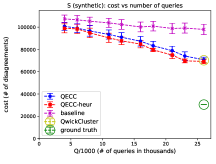
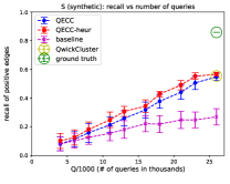
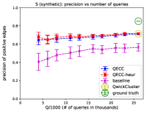
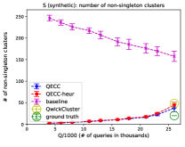
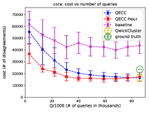
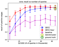
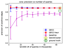
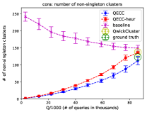
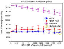
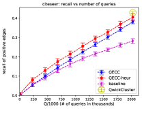
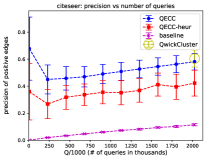
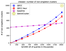
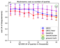
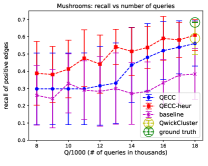
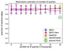
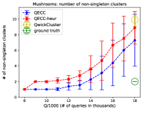
Figure 1. Accuracy measures of our two algorithms, the baseline, and ground truth on the datasets of Table LABEL:tab:datasets.

Synthetic graphs. We construct a family of synthetic graphs ${\mathcal{S}}=\{S(n,k,\alpha,\beta)\}$, parameterized by the number of vertices $n$, number of clusters in the ground truth $k$, imbalance factor $\alpha$, and noise rate $\beta$. The ground truth $T(n,k,\alpha)$ for $S(n,k,\alpha,\beta)$ consists of one clique of size $\alpha n/k$ and $k-1$ cliques of size $(1-\alpha)n/k$, all disjoint. To construct the input graph $S(n,k,\alpha,\beta)$, we flip the sign of every edge between same-cluster nodes in $T(n,k,\alpha)$ with probability $\beta$, and we flip the sign of every edge between distinct-cluster nodes with probability $\beta/(k-1)$. (This ensures that the number total number of positive and negative edges flipped is roughly the same.)

Real-world graphs. For our experiments with real-world graphs, we choose three with very different characteristics:

• The cora dataset, where each node is a scientific publication represented by a string determined by its title, authors, venue, and date. Following (Saha and Subramanian, 2019), nodes are joined by a positive edge when the Jaro string similarity between them exceeds or equals $0.5$.

• The Citeseer dataset, a record of publication citations for Alchemy. We put an edge between two publications if one of them cites the other (Yang et al., 2016).

• The Mushrooms dataset, including descriptions of mushrooms classified as either edible or poisonous, corresponding to the two ground-truth clusters. Each mushroom is described by a set of features. To construct the graph, we remove the edible/poisonous feature and place an edge between two mushrooms if they differ on at most half the remaining features. This construction has been inspired by (Gionis et al., 2007), who show that high-quality clusterings can often be obtained by aggregating clusterings based on single features.

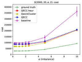
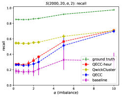
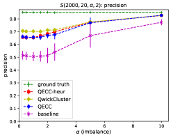
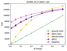
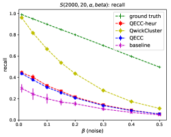
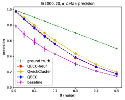
Figure 2. Effect of graph size $n$ (1rst row), number of clusters $k$, (2nd row), imbalance parameter $\alpha$ (3rd row) and noise parameter $\beta$ (4rth row) total cost and recall, for a fixed number $Q=15000$ of queries, except for QwickCluster.

Methodology. All the algorithms we test are randomized, hence we run each of them $50$ times and compute the empirical average and standard deviations of the total cost, precision and recall values. We compute the average number $A$ of queries made by QwickCluster and then run our algorithm with an allowance of queries ranging from $2n$ to $A$ at regular intervals.

We use synthetic graphs to study how cost and recall vary in terms of (1) number of nodes $n$; (2) number of clusters $k$; (3) imbalance parameter $\alpha$; (4) noise parameter $\beta$. For each plot, we fix all remaining parameters and vary one of them.

As the runtime for QECC scales linearly with the number of queries $Q$, which is an input parameter, we chose not to report detailed runtimes. We note that a simple Python implementation of our methods runs in under two seconds in all cases on an Intel i7 CPU at 3.7Ghz, and runs faster than the affinity propagation baseline we used (as implemented in Scikit-learn).

6.2. Experimental results

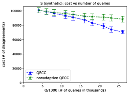
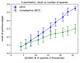
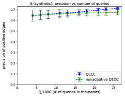
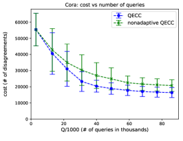
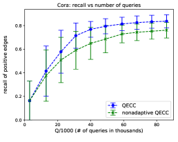
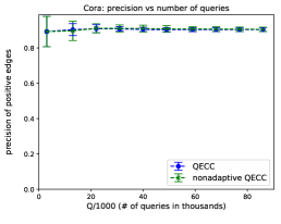
Figure 3. Comparison of QECC and its non-adaptive variant.

Table LABEL:tab:datasets summarizes the datasets we tested. Figure LABEL:fig:findings shows the measured clustering cost against the number of queries $Q$ performed by QECC and QECC-heur in the synthetic graph $S(2000,20,0.15,2)$ and the real-world Cora, Citeseer and Mushrooms datasets.

Comparison with the baseline. It is clearly visible that both QECC-heur and QECC perform noticeably better than the baseline for all query budgets $Q$. As expected, all accuracy measures are improved with higher query budgets. The number of non-singleton clusters found by QECC-heur and QECC increases with higher values of $Q$, but decreases when using the affinity-propagation-based baseline. We do not show this value for the baseline on Mushrooms because it is of the order of hundreds; in this case the ground truth number of clusters is just two, and QwickCluster, QECC and QECC-heur need very few queries (compared to $n$) to find the clusters quickly.

QwickCluster vs QECC and QECC-heur. At the limit, where $Q$ equals the average number $A$ of queries made by QwickCluster, both QECC and QECC-heur perform as well as QwickCluster. In our synthetic dataset, the empirical average cost of QwickCluster is roughly 2.3 times the cost of the ground truth, suggesting that it is nearly a worst-case instance for our algorithm since QwickCluster has an expected 3-approximation guarantee. Remarkably, in the real-world dataset cora, QECC-heur can find a solution just as good as the ground truth with just 40,000 queries. Notice that this is half what QwickCluster needs and much smaller than the $\binom{n}{2}\approx 1.7$ million queries that full-information methods for correlation clustering such as (Chawla et al., 2015) require.

Effect of graph characteristics. As expected, total cost and recall improve with the number of queries on all datasets (Figure LABEL:fig:findings); precision, however, remains mainly constant throughout a wide range of query budgets. To evaluate the impact of the graph and noise parameters on the performance of our algorithms, we perform additional tests on synthetic datasets where we fix all parameters to those of $S(2000,20,0.15,2)$ except for the one under study. Figure LABEL:fig:variation shows the effect of graph size $n$ (1st row), number of clusters $k$, (2nd row), imbalance parameter $\alpha$ (3rd row) and noise parameter $\beta$ (4th row) on total cost and recall, in synthetic datasets. Here we used $Q=15000$ for all three query-bounded methods: QECC, QECC-heur and the baseline. Naturally, QwickCluster gives the best results as it has no query limit. All other methods tested follow the same trends, most of which are intuitive:

• Cost increases with $n$, and recall decreases, indicating that more queries are necessary in larger graphs to achieve the same quality. Precision, however stays constant.

• Cost decreases with $k$ (because the graph has fewer positive edges). Recall stays constant for the ground truth and the unbounded-query method QwickCluster as it is essentially determined by the noise level, but it decreases with $k$ for the query-bounded methods. Again, precision remains constant except for the baseline, where it decreases with $k$.

• Recall increases with imbalance $\alpha$ because the largest cluster, which is the easiest to find, accounts for a larger fraction of the total number of edges $m$. Precision also increases. On the other hand, $m$ itself increases with imbalance, possibly explaining the increase in total cost.

• Finally, cost increases linearly with the level of noise $\beta$, while recall and precision decrease as $\beta$ grows higher.

Effect of adaptivity. Finally, we compare the adaptive QECC with Non-adaptive QECC as described at the end of Section LABEL:sec:main. Figure LABEL:fig:nonadaptive compares the performance of both on the synthetic dataset and on Cora. While both have the same theoretical guarantees, it can be observed that the non-adaptive variant of QECC comes at moderate increase in cost and, decrease in recall and precision.

7. Conclusions

This paper presents the first query-efficient correlation clustering algorithm with provable guarantees. The trade-off between the running time of our algorithms and the quality of the solution found is nearly optimal. We also presented a more practical algorithm that consistently achieves higher recall values than our theoretical algorithm. Both of our algorithms are amenable to simple implementations.

A natural question for further research would be to obtain query-efficient algorithms based on the better LP-based approximation algorithms (Chawla et al., 2015), improving the constant factors in our guarantee. Another intriguing question is whether one can devise other graph-querying models that allow for improved theoretical results while being reasonable from a practical viewpoint. The reason an additive term is needed in the error bounds is that, when the graph is very sparse, many queries are needed to distinguish it from an empty graph (i.e., finding a positive edge). We note that if we allow neighborhood oracles (i.e., given $v$, we can obtain a linked list of the positive neighbours of $v$ in time linear in its length), then we can derive a constant-factor approximation algorithm with $O(n^{3/2})$ neighborhood queries, which can be significantly smaller than the number of edges. Indeed, Ailon and Liberty (Ailon and Liberty, 2009) argue that with a neighborhood oracle, QwickCluster runs in time $O(n+OPT)$; if $OPT\leq n^{3/2}$ this is $O(n^{3/2})$. On the other hand, if $OPT>n^{3/2}$ we can stop the algorithm after $r=\sqrt{n}$ rounds, and by Lemma LABEL:lem:indep, we incur an additional cost of only $O(n^{3/2})=O(OPT)$. This shows that more powerful oracles allow for smaller query complexities. Our heuristic QECC-heur also suggests that granting the ability to query a random positive edge may help. These questions are particularly relevant to clustering graphs with many small clusters.

- (1)
- Ailon et al. (2008) Nir Ailon, Moses Charikar, and Alantha Newman. 2008. Aggregating inconsistent information: Ranking and clustering. J. ACM 55, 5 (2008), 1–27.
- Ailon and Liberty (2009) Nir Ailon and Edo Liberty. 2009. Correlation Clustering Revisited: The “True“ Cost of Error Minimization Problems. In Proc. of 36th ICALP. 24–36.
- Bansal et al. (2004) Nikhil Bansal, Avrim Blum, and Shuchi Chawla. 2004. Correlation Clustering. Machine Learning 56, 1-3 (2004), 89–113.
- Ben-Dor et al. (1999) Amir Ben-Dor, Ron Shamir, and Zohar Yakhini. 1999. Clustering Gene Expression Patterns. Journal of Computational Biology 6, 3/4 (1999), 281–297.
- Bonchi et al. (2013a) Francesco Bonchi, David García-Soriano, and Konstantin Kutzkov. 2013a. Local Correlation Clustering. Technical Report. arXiv preprint arXiv:1312.5105.
- Bonchi et al. (2014) Francesco Bonchi, David García-Soriano, and Edo Liberty. 2014. Correlation clustering: from theory to practice. In KDD. 1972. http://videolectures.net/kdd2014_bonchi_garcia_soriano_liberty_clustering/
- Bonchi et al. (2015) Francesco Bonchi, Aristides Gionis, Francesco Gullo, Charalampos Tsourakakis, and Antti Ukkonen. 2015. Chromatic correlation clustering. ACM Transactions on Knowledge Discovery from Data (TKDD) 9, 4 (2015), 34.
- Bonchi et al. (2013b) Francesco Bonchi, Aristides Gionis, and Antti Ukkonen. 2013b. Overlapping correlation clustering. Knowl. Inf. Syst. 35, 1 (2013), 1–32.
- Bressan et al. (2019) Marco Bressan, Nicolò Cesa-Bianchi, Andrea Paudice, and Fabio Vitale. 2019. Correlation Clustering with Adaptive Similarity Queries. Technical Report. arXiv preprint arXiv:1905.11902.
- Brody et al. (2011) Joshua Brody, Kevin Matulef, and Chenggang Wu. 2011. Lower bounds for testing computability by small width OBDDs. In International Conference on Theory and Applications of Models of Computation. Springer, 320–331.
- Charikar et al. (2005) Moses Charikar, Venkatesan Guruswami, and Anthony Wirth. 2005. Clustering with qualitative information. J. Comput. System Sci. 71, 3 (2005), 360–383.
- Chawla et al. (2015) Shuchi Chawla, Konstantin Makarychev, Tselil Schramm, and Grigory Yaroslavtsev. 2015. Near optimal LP rounding algorithm for correlationclustering on complete and complete k-partite graphs. In Proceedings of the forty-seventh annual ACM symposium on Theory of computing. ACM, 219–228.
- Demaine et al. (2006) Erik D. Demaine, Dotan Emanuel, Amos Fiat, and Nicole Immorlica. 2006. Correlation clustering in general weighted graphs. Theoretical Computer Science 361, 2-3 (2006), 172–187.
- Fischer (2004) Eldar Fischer. 2004. On the strength of comparisons in property testing. Information and Computation 189, 1 (2004), 107–116.
- Frey and Dueck (2007) Brendan J Frey and Delbert Dueck. 2007. Clustering by passing messages between data points. Science 315, 5814 (2007), 972–976.
- Gionis et al. (2007) Aristides Gionis, Heikki Mannila, and Panayiotis Tsaparas. 2007. Clustering aggregation. ACM Transactions on Knowledge Discovery from Data 1, 1, Article 4 (March 2007).
- Hassanzadeh et al. (2009) Oktie Hassanzadeh, Fei Chiang, Renée J. Miller, and Hyun Chul Lee. 2009. Framework for Evaluating Clustering Algorithms in Duplicate Detection. PVLDB 2, 1 (2009), 1282–1293.
- Kim et al. (2011) Sungwoong Kim, Sebastian Nowozin, Pushmeet Kohli, and Chang Dong Yoo. 2011. Higher-Order Correlation Clustering for Image Segmentation. In NIPS. 1530–1538.
- McCallum and Wellner (2005) Andrew McCallum and Ben Wellner. 2005. Conditional models of identity uncertainty with application to noun coreference. In Advances in neural information processing systems. 905–912.
- Ramachandran et al. (2007) Anirudh Ramachandran, Nick Feamster, and Santosh Vempala. 2007. Filtering spam with behavioral blacklisting. In Proceedings of the 14th ACM conference on Computer and communications security. ACM, 342–351.
- Saha and Subramanian (2019) Barna Saha and Sanjay Subramanian. 2019. Correlation Clustering with Same-Cluster Queries Bounded by Optimal Cost. Technical Report. arXiv preprint arXiv:1908.04976.
- Shamir et al. (2004) Ron Shamir, Roded Sharan, and Dekel Tsur. 2004. Cluster graph modification problems. Discrete Applied Mathematics 144, 1-2 (2004), 173–182.
- Wang et al. (2012) Jiannan Wang, Tim Kraska, Michael J Franklin, and Jianhua Feng. 2012. Crowder: Crowdsourcing entity resolution. Proceedings of the VLDB Endowment 5, 11 (2012), 1483–1494.
- Yang et al. (2016) Zhilin Yang, William W Cohen, and Ruslan Salakhutdinov. 2016. Revisiting semi-supervised learning with graph embeddings. In Proceedings of the 33rd International Conference on International Conference on Machine Learning, Vol. 48. 40–48.
- Yao (1977) Andrew Chi-Chin Yao. 1977. Probabilistic computations: Toward a unified measure of complexity. In 18th Annual Symposium on Foundations of Computer Science (FOCS 1977). IEEE, 222–227.