Electronic screening using a virtual Thomas–Fermi fluid for predicting wetting and phase transitions of ionic liquids at metal surfaces

Abstract

Of relevance to energy storage, electrochemistry and catalysis, ionic/dipolar liquids display unexpected behaviors — especially in confinement. Beyond adsorption, overscreening and crowding effects, experiments have highlighted novel phenomena such as unconventional screening and the impact of the electronic nature — metallic versus insulating — of the confining surface. Such behaviors, which challenge existing frameworks, highlight the need for tools to fully embrace the properties of confined liquids. Here, we introduce a novel approach describing electronic screening while capturing molecular aspects of interfacial fluids. While available strategies consider perfect metal or insulator surfaces, we build on the Thomas–Fermi formalism to develop an effective approach dealing with any imperfect metal between these asymptotes. Our approach describes electrostatic interactions within the metal through a ‘virtual’ Thomas-Fermi fluid of charged particles, whose Debye length sets the screening length $\lambda$. We show that this method captures the electrostatic interaction decay and electrochemical behavior upon varying $\lambda$. By applying this strategy to an ionic liquid, we unveil a wetting transition upon switching from insulating to metallic conditions.

Univ. Grenoble Alpes, CNRS, LIPhy, 38000 Grenoble, France

University of Stuttgart, Allmandring 3, 70569 Stuttgart, Germany

Laboratoire de Physique de l’Ecole Normale Supérieure, CNRS, Université PSL, Sorbonne Université, Sorbonne Paris Cité, Paris, France

e-mail: schlaich@icp.uni-stuttgart.de and benoit.coasne@univ-grenoble-alpes.fr

The fluid/solid interface as encountered in confined liquids is the locus of a broad spectrum of microscopic phenomena such as molecular adsorption, chemical reaction, and interfacial slippage.[1] These molecular mechanisms are key to nanotechnologies where the fluid/solid interaction specificities are harnessed for energy storage, catalysis, lubrication, depollution, etc. From a fundamental viewpoint, the behavior of nanoconfined fluids often challenges existing frameworks even when simple liquids are considered. Ionic systems, either in their liquid or solid state, between charged or neutral surfaces lead to additional ion adsorption, crowding/overscreening, surface transition, and chemical phenomena[2, 3, 4, 5] that are crucial in electrokinetics (e.g. electrowetting) and electrochemistry (e.g. supercapacitors/batteries).[6] Theoretical descriptions of nanoconfined fluids — except rare contributions[7, 8, 9, 10, 11, 12, 13, 14] — assume either perfectly metallic or insulating confining surfaces but these asymptotic limits do not fully reflect real materials as they display an intermediate imperfect metal/insulator behavior (only few metals behave perfectly and all insulators are semi-conducting to some extent). Yet, the electrostatic boundary condition imposed by the surrounding medium strongly impacts confined dipolar and, even more, charged systems.[15, 16, 17] For instance, the confinement-induced shift in the freezing of an ionic liquid was found to drastically depend on the surface metallic/insulating nature.[18]

Formally, quantum effects leading to electronic screening in the confining metallic walls can be accounted for using the microscopic Thomas–Fermi (TF) model.[19, 18] This formalism relies on a local density approximation for the charges in the metal which are treated as a free electron gas (therefore, restricting the electron energy to its kinetic contribution). This simple model allows considering any real metal — from perfect metal to insulator — through the Thomas–Fermi screening length $\lambda$. The latter is defined in terms of the electronic density of state of the metal at the Fermi level $\mathcal{D}(\mathcal{E}_{\mathrm{F}})$ according to $\lambda={\varepsilon}/{e^{2}\mathcal{D}(\mathcal{E}_{\mathrm{F}})}$ ($\varepsilon$ is the dielectric constant and $e$ the elementary charge); the Fermi energy is directly related to the free electron density $n_{0}$ as $\mathcal{E}_{\mathrm{F}}=\hbar^{2}(3\pi^{2}n_{0})^{2/3}/(2m_{e})$ where $m_{e}$ is the electron mass and $\hbar=h/2\pi$ the Planck constant, see Supplementary Information II A. Despite this available framework, the development of classical molecular simulation methods to understand the microscopic behavior of classical fluids in contact with imperfect metals is only nascent. While insulators are treated using solid atoms with constant charge, metals must be described using an effective screening approach. The charge image concept can be used for perfectly metallic and planar surfaces[20] but refined strategies must be implemented for non-planar surfaces such as variational[21, 22] or Gauss law[23, 24, 25] approaches to model the induced charge distribution in the metal. A recent proposal[8] builds on our TF framework[7] to propose a computational approach based on variational localized surface charges that accounts for electrostatic interactions close to imperfect metals.

Here, we develop an effective yet robust atom-scale simulation approach which allows considering the confinement of dipolar or charged fluids between metallic surfaces of any geometry and/or electronic screening length. Following Torrie and Valleau’s work for electrolyte interfaces,[26] the electronic screening in the imperfect confining metal is accounted for through the response of a high temperature virtual Thomas–Fermi fluid made up of light charged particles. Due to its very fast response, this effective Thomas–Fermi fluid mimics metal induction within the confining surfaces upon sampling the confined system configurations using Monte Carlo or molecular dynamics simulations. After straightforward implementation in existing simulation packages, this strategy provides a mean to impose a Thomas–Fermi screening length that is directly linked to the equivalent virtual fluid Debye length. By adopting a molecular level description, our approach captures all specificities inherent to confined and vicinal fluids at the nanoscale (e.g. density layering, slippage, non-viscous effects). This virtual Thomas–Fermi model correctly captures electrostatic screening within the confined system upon varying the confining host from perfect metal to insulator conditions. The presented molecular approach is also shown to accurately mimic the expected capacitive behavior, therefore opening perspectives for the atom-scale simulation of electrochemical devices involving metals of various screening lengths/geometries. To further assess this effective strategy, by considering the freezing of a confined ionic liquid, we show that the experimental behavior observed in Ref.[18] can be rationalized as the salt is predicted to melt at a temperature larger than the bulk melting point and that the shift in the melting point should increase with decreasing the screening length. Last but not least, using this novel method, by considering an ionic liquid between two parallel planes, we unravel a continuous wetting transition as the surfaces are tuned from insulating (non-wetting) to metallic (wetting).

A few remarks are in order. Formally, the impact of image forces induced in non-insulating solid surfaces when setting them in contact with charged and/or dipolar molecules was investigated in depth by Kornyshev and coworkers.[27, 28] Using a formal treatment of the Coulomb interactions with appropriate electrostatic boundary conditions, these authors have considered complex problems ranging from electric double layers[29, 30] to ion/molecule adsorption.[31, 32] This robust framework was employed for simple point charges but also for complex systems such as ionic liquids (whose chemical structure leads to ion-specific effects beyond electrostatic interactions). In contrast, the Thomas–Fermi model — which is at the heart of our molecular dynamics approach — is based on a simplified description of conductivity in solids. This simple formalism allows covering situations from perfect and imperfect metals to semiconductors by varying the screening length $\lambda$. The Thomas–Fermi model is known to be a rather crude approximation when describing the interaction between ions and solid surfaces.[33] In particular, due to the use of semi-quantum description level of charges in solids, it fails to accurately describe quantum effects such as Friedel oscillations, the image plane position and motion with respect to metal atoms, and the electron spillover outside the metal (a fortiori, the impact of charge adsorption at the solid surface is even more complicated to account for). As a result, in some cases such as for transition metals, metallic surfaces will not be appropriately described using the Thomas–Fermi approximation.

Yet, despite these drawbacks, as shown here, the Thomas–Fermi model provides a simple framework to implement the complex electrostatic interaction — including image forces — arising in the vicinity of metallic surfaces. Such multicontribution interaction, which results from a theoretical derivation described below (and in more detail in the Supplementary Information II), includes time demanding numerical estimates that cannot be calculated on the fly in molecular dynamics. As a result, despite its limitations and weaknesses, the Thomas–Fermi approach is an approximate scheme to account for electrostatic screening near solid surfaces with properties that range from perfectly metallic to insulating. In fact, in the present molecular approach, rather than formally implementing the equations corresponding to the Thomas–Fermi model, we rely on a simple effective procedure in which electrostatic screening induced by a fluid of charges located in the solid material is mapped onto the Thomas–Fermi length. As shown in this paper, we believe that this matching is a valid approach as the mapped screening length is consistent with the observed capacitance behavior of the system. Therefore, despite its simplicity, we believe that our effective molecular strategy provides a simple tool to investigate complex surface electrostatic phenomena occurring at solid/liquid interfaces. Even if this approach provides a first order picture (in the sense that some of the above mentioned aspects could be missing), the results reported below suggest that it captures striking phenomena such as the impact of screening length on capillary freezing. Among its strengths, this method allows considering nearly any screening length but also any electrode shape; indeed, by using a liquid phase of screening charges within the solid material, solid surfaces with complex morphology can be considered (this contrasts with other approaches which require defining an underlying atomic structure bearing localized polarizable electrons). Moreover, as it can be directly implemented in any standard molecular dynamics package, our approach can be used for fluids ranging from simple charged/dipolar molecules to more complex systems such as ionic liquids.

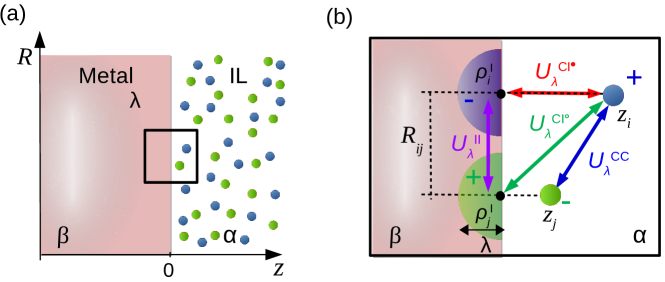
Figure 1: Electrostatic interactions in the vicinity of metal surfaces. (a) Ionic liquid (IL) in an insulating medium $\alpha$ close to an imperfect metal $\beta$ having a Thomas–Fermi length $\lambda$. (b) One and two-body interactions for two point charges $i,j$ at distances $z_{i}$ and $z_{j}$ from the surface and separated by in-plane distance $R_{\mathit{ij}}$. The induced charge distribution $\rho_{k}^{\mathrm{I}}(\mathbf{r})$ for $k=i,j$ (denoted by half-ellipsoids) within the metal is of opposite sign and decays over $\lambda$. The colored arrows show the different energy contributions given in Eq. 1.

Interaction at Thomas–Fermi metal interfaces
Fig. 1(a) depicts point charges in an insulating medium $\alpha$ of relative dielectric constant $\varepsilon_{\alpha}$ close to a metal $\beta$ of TF length $\lambda$. As shown in Supplementary Information II D, the electrostatic energy of two charges $i$ and $j$ at distances $z_{i}$ and $z_{j}$ from the dielectric/metal interface and separated by $r_{ij}=[R_{ij}^{2}+(z_{i}-z_{j})^{2}]^{1/2}$ with $R_{ij}$ the in-plane distance reads:

$$U_{\lambda}(z_{i},z_{j},R_{ij})=U^{\mathrm{CC}}(r_{ij})+U_{\lambda}^{\mathrm{CI}}(z_{i},z_{j},R_{ij})+U^{\mathrm{II}}_{\lambda}(z_{i},z_{j},R_{ij}).$$ (1)

where the superscripts C and I refer to the physical charges in the dielectric medium and induced charges within the metal, respectively. As shown in Fig. 1(b), $U^{\mathrm{CC}}$ is the Coulomb interaction energy between the charges $i$ and $j$ while $U^{\mathrm{II}}_{\lambda}$ is the interaction energy between the charge densities $\rho_{i}^{\mathrm{I}}$ and $\rho_{j}^{\mathrm{I}}$ induced in the metal by these two charges. For each ion $i$, its interaction energy $U_{\lambda}^{\mathrm{CI}}$ with the metal decomposes into a one-body contribution $U_{\lambda}^{\mathrm{CI}^{\bullet}}(z_{i})$ — corresponding to the interaction with its image in the metal — and two-body contributions $U_{\lambda}^{\mathrm{CI^{\circ}}}(z_{i},z_{j},R_{ij})$ — corresponding to the interaction with the induced charges due to all other charges $j$. Analytical expressions exist for $U_{\lambda}^{\mathrm{CI}^{\bullet}}$ and $U_{\lambda}^{\mathrm{CI^{\circ}}}$[9, 10, 11, 7] but $U^{\mathrm{II}}_{\lambda}$ must be estimated numerically from the energy density, i.e. $U^{\mathrm{II}}_{\lambda}=\int{\mathrm{d}}\mathbf{r}\Psi^{\mathrm{\beta}}_{i}(\mathbf{r})\rho^{\mathrm{I}}_{j}(\mathbf{r})+\Psi^{\mathrm{\beta}}_{j}(\mathbf{r})\rho^{\mathrm{I}}_{i}(\mathbf{r})$, where $\Psi^{\mathrm{\beta}}_{k}$ and $\rho^{\mathrm{I}}_{k}$ are the electrostatic potential and induced charge density in the metal due to the point charge $k=i,j$. All details are given in the Supplementary Information.

Effective molecular simulation approach
Except for the usual Coulomb energy CC, formal expressions for the CI and II energies cannot be implemented in molecular simulation due to their complexity. In particular, $U^{\mathrm{II}}_{\lambda}$ requires expensive integration on the fly as analytical treatment for imperfect metals is only available in closed forms in asymptotic limits.[14, 7] Here we model the resulting complex electrostatic interactions between the ions of the liquid thanks to a ‘virtual Thomas–Fermi fluid’ located within the confining solids, see Fig. 2(a). Our approach builds on the direct analogy between the Thomas–Fermi screening of electrons and the Debye–Hückel equation for electrolyte solutions. In the linear Thomas–Fermi formalism, the induced electronic charge density in the metal writes: $q_{\mathrm{TF}}\rho^{\mathrm{I}}(\mathbf{r})=-\varepsilon_{0}\varepsilon_{\beta}k_{\mathrm{TF}}^{2}\Psi_{\beta}(\mathbf{r})$ where $\varepsilon_{0}$ is the vacuum permittivity, $\varepsilon_{\beta}$ the relative dielectric constant, $k_{\mathrm{TF}}=[e^{2}\mathcal{D}(\mathcal{E}_{\mathrm{F}})/\varepsilon_{0}\varepsilon_{\beta}]^{1/2}$ the Thomas–Fermi wave-vector, and $\mathcal{D}(\mathcal{E}_{\mathrm{F}})$ the density of states at the Fermi level (see Supplementary Information II A). Combined with Poisson equation, this leads to the Helmholtz equation for TF screening, $\nabla^{2}\Psi_{\mathrm{II}}=k_{\mathrm{TF}}^{2}\Psi_{\mathrm{II}}$, which indeed resembles the Debye–Hückel equation for electrolyte solutions. Accordingly, one can simulate the imperfect metal using a system of virtual (classical) charged particles of charge $q_{\mathrm{TF}}$ and mass $m_{\mathrm{TF}}$, with density $\rho_{\mathrm{TF}}$ and temperature $T_{\mathrm{TF}}$. The analogous TF screening length $\lambda=k_{\mathrm{TF}}^{-1}$ can be identified as the equivalent Debye length $\lambda_{\mathrm{D}}$:

$$\lambda\sim\lambda_{\mathrm{D}}=\sqrt{\frac{\varepsilon_{\beta}\varepsilon_{0}k_{\textnormal{B}}T_{\mathrm{TF}}}{\rho_{\mathrm{TF}}q_{\mathrm{TF}}^{2}}}.$$ (2)

Hence, by considering the dynamics of these light ions located in the confining solid, any screening length $\lambda$ between 0 (perfect metal) and $\infty$ (insulator) can be efficiently mimicked depending on $q_{\mathrm{TF}}$, $\rho_{\mathrm{TF}}$, and $T_{\mathrm{TF}}$. This virtual system allows simulating the complex electrostatic interactions within the ionic liquid in the vicinity of an imperfect metal.

As mentioned in the previous paragraph, by tuning the different parameters inherent to the Thomas–Fermi fluid — namely, the fluid particle charge $q_{\mathrm{TF}}$, temperature $T_{\mathrm{TF}}$ and density $\rho_{\mathrm{TF}}$ — confining solids with an electrostatic screening length ranging from metallic to insulating can be mimicked. Yet, Eq. 2 shows that mapping the fluid of mobile charges onto the TF model only requires to set a single parameter $\rho_{\mathrm{TF}}q_{\mathrm{TF}}^{2}/T_{\mathrm{TF}}$ (fixing $\varepsilon_{\beta}=1$). In practice, while this implies that different combinations for these parameters can lead to the same effective screening, there are a few constraints that should be verified. First, as discussed hereafter in this paragraph, to account for the ultra-fast dynamical relaxation of charges in the solid compared to that in the confined salt, the Thomas–Fermi temperature $T_{\mathrm{TF}}$ is chosen to be very large. While this is important to capture the order of magnitude difference between these two timescales, this implies that two thermostats have to be used to properly regulate the temperature of the two subsystems. In this regard, we emphasize that the results reported here were obtained using either a Nose-Hoover thermostat or a Langevin thermostat (however, it was found that a Langevin thermostat is recommended as it ensures that the two subsystems display uncoupled homogeneous/constant temperatures). Moreover, in contrast to the temperature of the confined charges, $T_{\mathrm{TF}}$ should not be seen as a physical temperature but rather as a parameter governing the Thomas–Fermi fluid dynamics and, hence, effective screening. Second, since the ionic force in the Debye length is directly the product of the squared charge and density, i.e. $\rho_{\mathrm{TF}}q_{\mathrm{TF}}^{2}$, one can tune the effective screening in the metal by tuning either one or two of these parameters. In practice, after conducting several tests, we found it more efficient to keep the number and, hence, the density of charges in the Thomas–Fermi fluid constant. Indeed, on the one hand, playing with $q_{\mathrm{TF}}$ at constant $\rho_{\mathrm{TF}}$ offers more flexibility in tuning the screening length. On the other hand, treating very imperfect metals with constant $q_{\mathrm{TF}}$ would require considering a very small number of Thomas–Fermi ions leading to poor sampling/statistics performance. Before going into more technical details, we emphasize that the exact choice of parameters made to mimic different screening lengths is expected to impact the dynamics/kinetics of the observed phenomena (by setting a given temperature $T_{\mathrm{TF}}$, we do impose a relaxation time). However, like in classical thermodynamics, we do not expect this effective relaxation within the virtual Thomas–Fermi fluid to affect the equilibrium properties of the charged liquid confined between the metallic surfaces.

In more detail, in our molecular dynamics approach, to ensure that the particles in the effective Thomas–Fermi fluid relax fast, their mass/temperature are chosen much smaller/larger than their counterpart in the confined system; typically $m_{\mathrm{TF}}\sim 0.01m$ and $T_{\mathrm{TF}}\sim 10T$ (requiring typical integration steps of 0.1 fs and 1 fs, respectively). In practice, as shown in Fig. 2(a), the effective simulation strategy consists of sandwiching the charged or dipolar system between two metallic media separated by a distance $d_{\mathrm{w}}$. The confining media of width $d_{\mathrm{TF}}$ are filled with the Thomas–Fermi fluid having a density $\rho_{\mathrm{TF}}$. Once $\rho_{\mathrm{TF}}$ and $T_{\mathrm{TF}}$ are set, $\lambda_{\mathrm{D}}$ is varied by tuning $q_{\mathrm{TF}}$ according to Eq. 2; from $q_{\mathrm{TF}}=0$ $(\lambda_{\mathrm{D}}\rightarrow\infty$) for an insulator to $q_{\mathrm{TF}}=1$ ($\lambda_{\mathrm{D}}=0.03\,\mathrm{nm}$) for a nearly perfect metal. All simulations reported in this article are carried out using molecular dynamics but they could be easily implemented into Monte Carlo algorithms to perform calculations in other ensembles (Grand Canonical and isothermal/isobaric ensembles for instance). All simulation details are provided in the Methods section. Since we consider a set of explicit charges with no solvent to model the Thomas–Fermi fluid, we used consistently a relative dielectric permittivity equal to 1. However, this raises the question of the true dielectric constant of the solid material that we intend to mimic. Describing s-p metals using a Thomas–Fermi model is usually done by accounting for the dielectric constant of the underlying ion structure in the metal. Such dielectric background, which arises from the polarizability of the core electron shells around each metal atom, differs from one metal to another (with values of the order of one to a few times the vacuum dielectric permittivity). In semiconductors, such a dielectric background, in which the outer electrons move, arises from interband transitions with values that can be close to 10. As another example, when modeling semi-metals, a large Thomas–Fermi screening length is used together with a large dielectric constant to account for the low charge carrier concentration and absence of band-gaps, respectively. In this context, we mention that the dielectric constant in semi-metals can be evaluated by considering the electron density of states as proposed by Gerischer and coworkers.[34, 35] These specific yet representative examples illustrate that the nature of the solid material manifests itself in the Thomas–Fermi screening length but also in the dielectric constant. While this duality (screening/dielectric properties) is of course of prime importance when modeling the complex physics of metallic and semiconducting surfaces, we simplify the problem in the present approach as we only aim at mimicking in an effective but quantitative fashion the electrostatic screening induced by the solid surface on the confined or vicinal charges. To this end, as already introduced above, our proposed molecular approach adopts a different view by mimicking a liquid of charges to produce an effective screening that corresponds to an underlying Thomas–Fermi model — this is what is referred to in our article as ‘virtual’ Thomas–Fermi fluid. In other words, as will be shown below, by calculating the induced electrostatic screening length, we can map this pseudo Thomas–Fermi medium onto practical situations by establishing a consistent relation between its Debye length $\lambda_{\textrm{D}}$ and the induced electrostatic screening length $\lambda$. Therefore, we are not attempting per se to implement the electrostatic screening equations as derived using the Thomas–Fermi formalism. In this regard, as will be established later, we believe that our mapping procedure is sound and robust as the inferred screening length is found to be consistent with that corresponding to the observed capacitance behavior of our system.

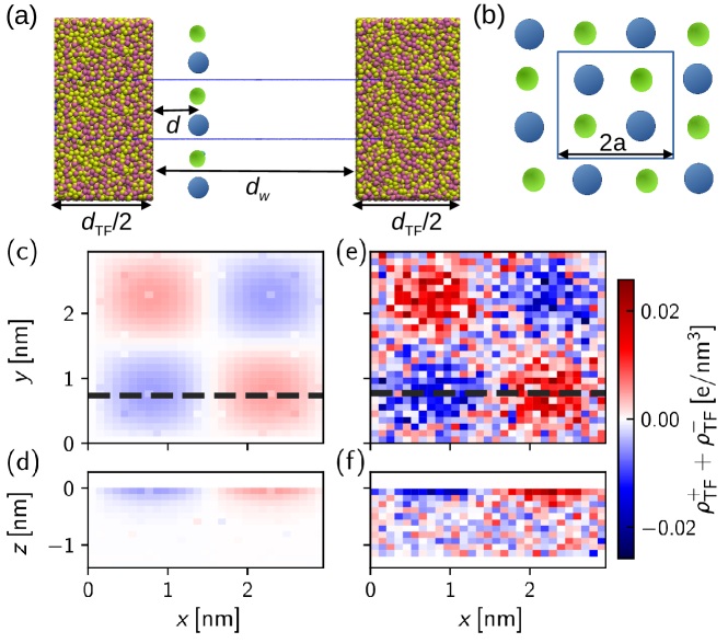
Figure 2: Induced charges and screening at metallic surfaces. (a) 2D ionic crystal (blue/green charges) at a distance $d=0.22\,\mathrm{nm}$ from a medium in which electrostatic screening is modeled using a Thomas–Fermi fluid (yellow/pink charges). The crystal layer is confined in a pore of width $d_{\mathrm{w}}$ while the Thomas–Fermi fluid occupies a region of width $d_{\mathrm{TF}}$. (b) Top view of the 2D ionic crystal (lattice constant $a$) illustrating the periodic boundary conditions. (c)-(d) Top/side views of the induced charge density $\rho^{\mathrm{I}}(d,\mathbf{r})$ in a Thomas–Fermi fluid as obtained from Eq. 3 for the system in (a). (e)-(f) Same as (c)-(d) but using our simulation approach. The screening length as defined in Eq. 2 is $\lambda=0.25\,\mathrm{nm}$.

2D crystal at metallic interfaces
To validate our effective approach, we consider a 2D square crystal of lattice constant $a=1.475\,\mathrm{nm}$ made up of charges $\pm 1\,\mathrm{e}$ and located at a distance $d$ from a metal (Fig. 2). Due to the periodic boundary conditions, a second pore/metal interface is present at a distance $d_{\mathrm{w}}=20\,\mathrm{nm}$. Yet, as shown in Supplementary Figure S9, this second interface does not affect the electrostatic energy as $d_{\mathrm{w}}$ is large enough. In the Thomas–Fermi framework, the charge density $\rho^{\mathrm{I}}$ at a position $\mathbf{r}$ in the metal induced by a charge $q$ located in $(0,0,d)$ reads (see Supplementary Information II D):

$$\rho^{\mathrm{I}}(d,z,R)=-\int\limits_{0}^{\infty}{\mathrm{d}}KKJ_{0}(KR)\frac{\varepsilon_{\beta}k_{\mathrm{TF}}^{2}q{\mathrm{e}}^{-Kd}}{2\pi\left(\varepsilon_{\alpha}K+\varepsilon_{\beta}\kappa\right)}{\mathrm{e}}^{\kappa z},$$ (3)

where $R=[x^{2}+y^{2}]^{1/2}$ is the lateral distance to the charge $q$, $J_{0}$ is Bessel function of the first kind, and $\kappa^{2}=K^{2}+k_{\mathrm{TF}}^{2}$. Figure 2(c,d) shows the induced charge density $\rho^{\mathrm{I}}(d,\mathbf{r})$ as obtained by summing Eq. 3 for the 2D crystal when $d=0.22\,\mathrm{nm}$ and $\lambda_{\mathrm{D}}=k_{\mathrm{TF}}^{-1}=0.25\,\mathrm{nm}$ (as discussed in Supplementary Information III, Eq. 3 must be summed over all crystal periodic images but it was found that the sum converges quickly). For comparison, Fig. 2(e,f) shows $\rho^{\mathrm{I}}(d,\mathbf{r})$ as obtained using our effective approach from the local charge density in the metal, i.e. $\rho^{\mathrm{I}}=e(\rho_{\mathrm{TF}}^{+}-\rho_{\mathrm{TF}}^{-})$. In contrast to $\rho^{\mathrm{I}}(d,\mathbf{r})$ in the Thomas–Fermi model, due to their finite size, the fluid charges in the simulation cannot approach arbitrarily close to the metal/pore surface. For consistency, the analytical/simulation data were compared by defining $z=0$ in the simulation as the position where the Thomas–Fermi fluid density becomes non-zero. Fig. 2 shows that the effective molecular simulation qualitatively captures the predicted density distribution induced in the metal. Each physical charge in the 2D crystal induces in the metal a diffuse charge distribution of opposite sign. Moreover, as expected from the Thomas–Fermi framework, the induced charge distribution in the effective simulation decays over the typical length $\lambda_{\mathrm{D}}$.

Our effective approach was assessed quantitatively by probing the energy of the 2D ionic crystal as a function of its distance $d$ to the metal surface for different screening lengths $\lambda$. The simulated electrostatic energy $U_{\lambda}(d)$ consists of all ion pair contributions in Eq. 1 as discussed in Supplementary Information V. Figure 3 compares the total energy $U_{\lambda}$ as a function of the distance $d$ with the numerically evaluated prediction from Eq. 1. As expected theoretically, the overall energy decays with decreasing $\lambda$ between boundaries for an insulator ($\lambda\to\infty$) and a perfect metal ($\lambda\to 0$). As shown in Fig. 3, our effective approach captures quantitatively the screening behavior of the confining medium assuming a screening length $\lambda=c_{0}+c_{1}\lambda_{\mathrm{D}}+c_{2}\lambda_{\mathrm{D}}^{2}$ (with $\lambda_{\mathrm{D}}$ the ion gas Debye length, $c_{0}=0.22\,\mathrm{nm}$, $c_{1}=0.91$ and $c_{2}=0.28\,\mathrm{nm}^{-1}$ in our system). Such values do not simply correspond to fitting parameters that allow matching the simulated and theoretical energies; as explained in the next paragraph, they were derived so that the capacitance of the virtual Thomas–Fermi fluid matches the theoretically expected value $C=\varepsilon_{0}/\lambda$. The fact that the rescaled screening length $\lambda$ also allows recovering the expected screened interaction energy further supports the physical validity of our effective molecular approach. Moreover, physically, the parameters $c_{0}$, $c_{1}$, and $c_{2}$ are not just empirical parameters as they account for the following effects in the screening fluid used in the simulation: $c_{0}$ accounts for the finite size $\sigma$ of the Thomas–Fermi ions which prevents reaching screening $\lambda\leq\sigma$. This is supported by the fact that $c_{0}\sim\sigma$ corresponds to the value below which the repulsive interaction potential in the Thomas–Fermi fluid becomes larger than $k_{\textrm{B}}T$. $c_{1}$ arises from the non-ideal behavior of the effective Thomas–Fermi fluid which leads to overcreening compared to an ideal gas having the same charge density $\rho_{\mathrm{TF}}$ ($c_{1}=1$ corresponds to the ideal behavior); $c_{2}\neq 0$ indicates non-linear effects in electrostatic screening which go beyond the linear approximation used in the Thomas–Fermi framework.

To illustrate the ability of our approach to capture the impact of various screening lengths — from insulators to metallic surfaces — on electrostatic interactions, we show in Supplementary Fig. S1(a) the electrostatic energy arising from image/charge interactions, $U^{\mathrm{CI}}(\lambda)$, for a molten salt confined between two solid surfaces as a function of the electrostatic screening length $\lambda$. To probe the impact of such interactions with induced charges, a fixed liquid configuration was considered as it implies that the direct coulomb interaction $U^{\mathrm{CC}}(\lambda)$ is constant. As expected, upon decreasing $\lambda$, the overall electrostatic energy decreases as the interactions with the induced charges in the metallic surfaces become more negative. Moreover, by extrapolating $U^{\mathrm{CI}}(\lambda)$ to perfect metallic conditions (i.e. $\lambda\to 0$), one recovers the expected charge image contribution corresponding to half of the Coulomb energy. Such data show that our molecular simulation strategy does mimic — albeit in an effective fashion — the electrostatic screening induced by metallic surfaces. In this respect, we emphasize that this approach can be extended to almost any surface geometry/topology. First, this versatile model does not require inputting an underlying atomic structure for the surface (by describing the charges in the metal as a fluid, one needs not to consider an atomic lattice to which charges are linked). Second, any geometry from a simple flat or cylindrical surface to disordered/rough surfaces can be considered as it simply requires to encapsulate the screening charges within a mathematically defined region. Correctly accounting for image forces near solid surfaces is crucial to capture the rich and complex behavior of confined charges. In particular, as theoretically predicted by Kondrat and Kornyshev,[36] it has been observed using molecular simulation that such image forces can lead to superionic states — where like-charge pairs form — in metallic nanoconfinement.[37] In this respect, it was found that electron spillover leads to effective pore sizes narrower than the nominal pore size. While the Thomas–Fermi model was found to fail to predict this effective pore size reduction,[38, 39] we believe that — at least as a first order approach — the results reported in the present paper show that our molecular strategy can be used to capture the impact of electrostatic screening on ions between metallic surfaces. In particular, by comparing molecular simulation for an ionic liquid on a perfect metal surface at constant potential and constant charge, it was recently shown that image forces are screened on such a very short scale that they do not affect the adsorbed liquid.[40] This highlights the need to consider effective molecular simulation approaches such as the one reported in this paper to consider imperfect metals and, hence, larger screening lengths corresponding to many experimental situations.

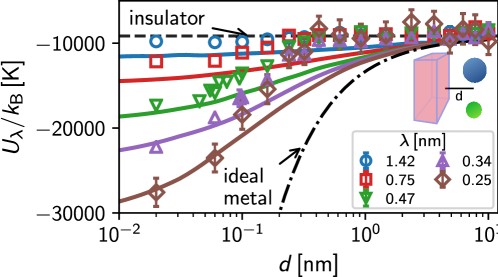
Figure 3: Screened electrostatic interactions through the use of a virtual Thomas–Fermi fluid. Electrostatic energy $U_{\lambda}(d)$ between a 2D ionic crystal and a Thomas–Fermi metal separated by a distance $d$ for different $\lambda$. For each $\lambda$, the symbols correspond to the effective simulation while the solid line shows the linear Thomas–Fermi predictions.

Capacitance
To further establish the validity of our novel molecular approach, an important requirement is to verify that the virtual Thomas–Fermi fluid yields the correct capacitance behavior. With this aim, as shown in Fig. 4(a), a simple molecular dynamics set-up was designed by assembling a composite system made up of two Thomas–Fermi fluids sandwiching a dielectric material of a width $d_{\mathrm{w}}$ (either a vacuum layer or a molten salt was considered to verify that the overall capacitance follows the expected physical behavior). The molten salt (NaCl) is modeled using charged particles $\pm 1{\mathrm{e}}$ that interact via a Born–-Mayer–-Huggins potential[41] (see Supplementary Table S1). To prevent mixing of the Thomas–Fermi fluid/charged system, a reflective wall of thickness $\xi=0.2$ nm is positioned between the two subsystems. The whole composite is placed between two electrodes having an overall charge $+Q$ and $-Q$ (all details can be found in the Methods section). With such a geometry, the capacitance $C=Q/\Delta\Psi$ is readily obtained from the potential difference $\Delta\Psi$. As shown in Fig. 4(a), with this molecular simulation set-up mimicking in a simplified yet realistic way an experimental electrochemical cell, we can perform a molecular dynamics simulation to readily estimate the positive and negative charge density profiles within the confined salt [$\rho_{+}(z)$ and $\rho_{-}(z)$]. Using Poisson equation, i.e. $\Delta\Psi(z)=-\rho(z)/\epsilon$ with $\rho(z)=e[\rho_{+}(z)-\rho_{-}(z)]$, $\Delta\Psi(z)$ is determined by integrating twice the charge density profile $\rho(z)$. Fig. 4(a) shows $\Delta\Psi(z)$ as a function of the position $z$ within the confined liquid for different screening lengths $\lambda$. In practice, two simple situations are considered; the porosity between the two metallic surfaces is either occupied by vacuum or by a molten salt. As expected, $\Delta\Psi$ increases with increasing $z$ as the negative electrode is located at $z=0$ (positive charge adsorption) and the positive electrode is located at $z=d_{\mathrm{w}}$ (negative charge adsorption). Moreover, by considering the data sets for vacuum-filled and liquid-filled pores in Fig. 4(a), we observe that the slope of $\Delta\Psi(z)$ in the pore region is larger for the former than for the latter. Considering that $C=Q/\Delta\Psi$, this result suggests that as expected the sandwiched salt layer has a larger capacitance than the sandwiched vacuum layer. To provide a more quantitative picture of the system capacitance as a function of the screening length $\lambda$, we performed in the following paragraph a more detailed analysis in which the capacitance of the different elements — confined material and Thomas–Fermi fluid — is extracted.

The system considered here simply consists of double layer capacitors in series so that its capacitance per unit area should verify the following combination rule:

$$\frac{1}{C}=\frac{1}{C_{\mathrm{vac}}}+\frac{2}{C_{\mathrm{TF}}}=\frac{d_{\mathrm{w}}+2e}{\varepsilon_{0}}+\frac{2\lambda}{\varepsilon_{0}},$$ (4)

where the first and second terms correspond to the capacitance of the vacuum slab of width $d_{\mathrm{w}}$ and that of the Thomas–Fermi fluid (the factor 2 simply accounts for the presence of two Thomas–Fermi/vacuum interfaces). As shown in Fig. 4(b), the simulation data are in reasonable agreement with the prediction from this simple expression with deviations increasing with $\lambda$. Interestingly, as shown in the insert in Fig. 4(b), our effective approach captures quantitatively the expected capacitance behavior of the confining medium upon rescaling $\lambda_{\mathrm{D}}\to\lambda=c_{0}+c_{1}\lambda_{\mathrm{D}}+c_{2}\lambda_{\mathrm{D}}^{2}$ (see discussion above). As another consistency check, the vacuum layer in the capacitor was replaced by a slab of molten salt — see molecular configuration shown in Fig. 4(a). As expected, upon inserting such a molten salt, the effective capacitance $C$ drastically increases (i.e. the inverse capacitance shown in Fig. 4(b) decreases). More importantly, as shown in Fig. 4(c), the induced capacitance change $\Delta 1/C$ observed in our simulation data follow the expected behavior with a $\lambda$-independent value:

$$\Delta 1/C=d_{\mathrm{w}}\frac{\varepsilon-\varepsilon_{0}}{\varepsilon\varepsilon_{0}},$$ (5)

where $\varepsilon$ is the permittivity of the molten salt. Furthermore, since $\varepsilon\gg\varepsilon_{0}$, we predict that $\Delta 1/C\sim d_{\mathrm{w}}/\varepsilon_{0}$ in very good agreement with the simulation data shown as green circles in Fig. 4(c) (the small deviation is due to the fact that the vacuum permittivity is not completely negligible compared to that of the molten salt).

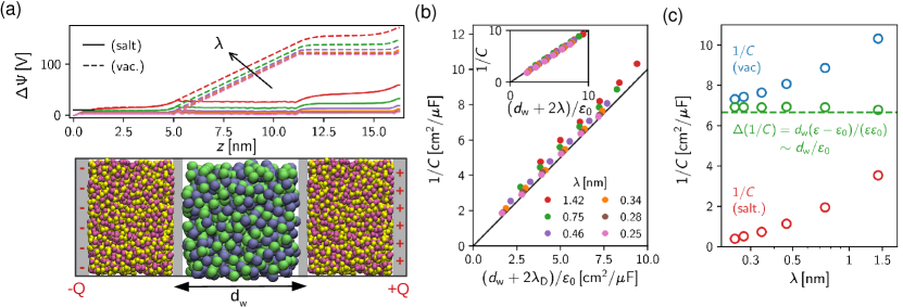
Figure 4: Capacitive behavior of virtual Thomas–Fermi fluids. (a) Typical molecular configuration of the molecular dynamics set-up employed to determine the capacitive behavior of the virtual Thomas–Fermi fluid. A molecular system — here, a molten salt corresponding to the blue/green spheres — is confined between two virtual Thomas–Fermi fluids (yellow/pink spheres). This composite system is sandwiched by two electrodes having a constant surface charge $\pm Q$. As shown in the top figure, using this set-up, the electrostatic potential profile $\Delta\Psi(z)$ can be determined by integrating twice the resulting charge density profile $\rho(z)=e[\rho_{+}(z)-\rho_{-}(z)]$. Such numerical assessments were performed for different screening lengths $\lambda$ where the confined material is either a vacuum layer (dashed lines) or a molten salt (solid lines). (b) Reciprocal capacitance $1/C$ of the empty Thomas–Fermi capacitor for different $\lambda_{\mathrm{D}}$ versus the analytical prediction for two double layer capacitors in series. The inset shows that the simulation data collapse onto the same master curve when plotted using the effective screening length $\lambda$. (c) Reciprocal capacitance $1/C$ as a function of the screening length $\lambda$ for a capacitor made up of vacuum (red symbols) or molten salt (blue symbols) confined between the TF fluids. As expected, for $\varepsilon=\varepsilon_{\alpha}\varepsilon_{0}\gg\varepsilon_{0}$, the difference between both systems (green symbols) is close to $d_{\mathrm{w}}/\varepsilon_{0}$.

Capillary freezing/melting in confinement
In what precedes, our effective molecular approach was shown to capture the electrostatic energy predicted using the Thomas–Fermi formalism for electrostatic screening in metallic materials as well as the capacitive behavior of a molten salt sandwiched between metallic surfaces with different screening lengths. Yet, in addition to these two validation steps, it should be verified that our simple strategy allows reproducing available experimental data for realistic materials. To do so, we have performed additional calculations using our effective treatment to study the liquid/crystal phase transition in various metallic confinements as experimentally reported by Comtet et al.[18] By considering the crystallization of an ionic liquid confined between an AFM tip and a metallic surface, these authors showed that the melting temperature is shifted above the bulk melting point and that the shift in the melting point increases with decreasing the screening length. To help rationalize these results, we performed the following molecular simulation study using our effective electrostatic screening strategy in confined charged systems.

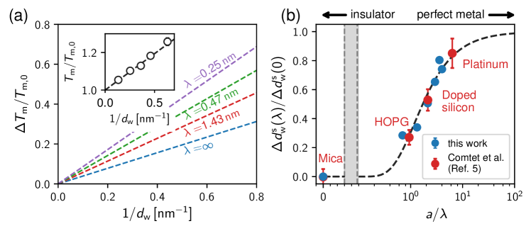
Figure 5: Capillary freezing at metallic surfaces. (a) Shift in the melting point $\Delta T_{m}$ with respect to the bulk melting temperature $T_{\mathrm{m},0}$ for a salt confined between two flat surfaces separated by a distance $d_{\textrm{w}}$. The confining surfaces are made up of different types of materials characterized by their electrostatic screening length $\lambda$: from insulator ($\lambda\to\infty$) to more and more perfect metals ($\lambda=$ 1.43, 0.47, and 0.25 nm). The insert shows the melting point $T_{\mathrm{m}}$ normalized to the bulk melting point $T_{\mathrm{m},0}$ as a function of the reciprocal pore size $d_{\textrm{w}}^{-1}$ as obtained from the direct coexistence method for insulating surfaces. (b) Shift induced in the capillary freezing length $\Delta d_{\textrm{w}}^{\textrm{s}}(\lambda)=d_{\textrm{w}}^{\textrm{s}}(\lambda)-d_{\textrm{w}}^{\textrm{s}}(\infty)$ for a salt confined between two surfaces characterized by their electrostatic screening length $\lambda$. The data are plotted with respect to the value obtained for an insulating surface $d_{\textrm{w}}^{\textrm{s}}(\infty)$. The blue circles are simulation data for a simple molten salt while the red circles are the experimental data by Comtet et al. who considered the capillary freezing of a room temperature ionic liquid [BMIM]/[BF4] confined between different materials as labeled in the figure. The dashed line corresponds to the predictions obtained by fitting the data $\Delta\gamma(\lambda)$.

First, by considering insulating surfaces, we use the direct coexistence method (DCM) in which a crystalline salt coexists with its molten salt in a slit pore of a size $d_{\mathrm{w}}$ (various pore widths between 1.5 and 7.1 nm were considered). To mimic a physical system in which the confined phases also interact through simple dispersive/repulsive interactions with the surface, a 9-3 Lennard-Jones interaction potential was added between each salt atom and the solid surface. The use of such structureless surfaces to describe the confining solids was made to avoid inducing a peculiar crystalline structure by employing a given molecular periodic lattice. Moreover, to ensure that such dispersive interactions do not impact too much the melting point in confinement, the potential wall depth was chosen of the order of $k_{\textrm{B}}T$ and, hence, at a value much lower than the electrostatic interactions. Using this set-up, molecular dynamics simulations in the canonical ensemble are performed for different $T$ to determine the melting temperature $T_{\mathrm{m}}$ as follows. The crystalline salt melts into the liquid phase for $T>T_{\mathrm{m}}$ while the molten salt crystallizes into the crystal phase for $T<T_{\mathrm{m}}$. The insert in Fig. 5(a) shows the shift in the melting point with respect to the bulk melting point, $\Delta T_{\mathrm{m}}=T_{\mathrm{m}}-T_{\mathrm{m,0}}$ as a function of pore size $d_{\mathrm{w}}$. In agreement with the experimental data,[18] these data show that the salt confined between insulating surfaces has a melting temperature above the bulk melting point. Moreover, the melting point shift $\Delta T_{\mathrm{m}}/T_{\mathrm{m,0}}$ is found to scale with the reciprocal pore size $1/d_{\mathrm{w}}$ as predicted using the Gibbs-Thomson equation, $\Delta T_{\mathrm{m}}/T_{\mathrm{m,0}}=[2\Delta\gamma(\infty)]/[\rho_{\mathrm{c}}\Delta H_{\mathrm{m}}d_{\mathrm{w}}]$, where $\rho_{\mathrm{c}}$ is the crystalline density, $\Delta H_{\mathrm{m}}$ the latent heat of melting, and $\Delta\gamma(\infty)=\gamma_{\mathrm{lw}}(\infty)-\gamma_{\mathrm{cw}}(\infty)$ the surface tension difference for the crystal/surface and liquid/surface interfaces. Considering the values measured from our molecular simulation ($\rho_{\mathrm{c}}=37.2\,\mathrm{mol/l}$ and $\Delta H_{\mathrm{m}}=27.9\,\mathrm{kJ/mol}$), fitting $\Delta T_{\mathrm{m}}/T_{\mathrm{m,0}}$ against $1/d_{\textrm{w}}$ leads to $\Delta\gamma(\infty)\sim 0.34\,\mathrm{J/m^{2}}$. To assess the impact of the electrostatic screening length $\lambda$ on capillary freezing, we use the following expression in which the liquid/surface and crystal/surface interfacial tensions between the metallic surface and the crystal ($x=\mathrm{c}$) or the liquid ($x=\mathrm{l}$) is given by its value for the insulating surface corrected for the charge-image interactions $U^{\textrm{CI}}(\lambda)$: $\gamma_{x\mathrm{w}}(\lambda)=\gamma_{x\mathrm{w}}(\infty)+\rho_{x}\ell U^{\textrm{CI}}(\lambda)$, where $\ell$ is a scaling length that converts a volume energy $U^{\textrm{CI}}$ into a surface energy. As shown Supplementary Fig. 1(b), such a simple relationship reasonably captures the impact of electrostatic screening on the liquid/surface interfacial tension which was assessed using independent simulation through the Irving-Kirkwood formalism: $\gamma(\lambda)=L_{z}/2\langle P_{\mathrm{N}}-P_{\mathrm{T}}\rangle$, where the terms in bracket are the average normal and tangential pressures, $L_{z}$ is the box length in the $z$ direction and the factor 2 accounts for the two interfaces in the slit geometry. Despite the fact that the simple expression $\gamma(\lambda)\sim\rho U^{\textrm{CI}}(\lambda)$ neglects the impact of screening on the entropy of the liquid, it provides an accurate description of the surface tension change induced by electrostatic screening in the metallic surfaces (we note that this simple equation holds even better for the crystalline phase as its entropy is negligible). This allows writing that $\Delta\gamma(\lambda)=\Delta\gamma(\infty)+(\rho_{\mathrm{l}}-\rho_{\mathrm{c}})\ell U^{\textrm{CI}}(\lambda)$. As shown in Fig. 5(a), considering that $U^{\textrm{CI}}(\lambda)<0$ becomes more negative upon decreasing $\lambda$ and $\rho_{\mathrm{c}}>\rho_{\mathrm{l}}$, this simple scaling predicts that the shift in the melting point $\Delta T_{\mathrm{m}}/T_{\mathrm{m,0}}$ increases as the surfaces turn from insulating to metallic.

To confront our results with the experimental data on capillary freezing,[18] Fig. 5(b) shows the impact of the screening length $\lambda$ on the capillary pore size $d_{\textrm{w}}^{\mathrm{s}}(\lambda)=[2\Delta\gamma(\lambda)T_{\mathrm{m,0}}]/[\rho_{\mathrm{c}}\Delta H_{\mathrm{m}}\Delta T_{\mathrm{m}}]$ below which salt crystallization is observed. In more detail, to compare quantitatively our data with those obtained experimentally for a room temperature ionic liquid, we plot the shift induced by surface metallicity in this capillary pore size with respect to that for an insulating surface $\Delta d_{\textrm{w}}^{\mathrm{s}}(\lambda)$ where $\Delta d_{\textrm{w}}^{\mathrm{s}}(\lambda)=d_{\textrm{w}}^{\mathrm{s}}(\lambda)-d_{\textrm{w}}^{\mathrm{s}}(\infty)$. The choice to normalize $\Delta d_{\textrm{w}}^{\mathrm{s}}(\lambda)$ in Fig. 5(b) by $\Delta d_{\textrm{w}}^{\mathrm{s}}(0)=d_{\textrm{w}}^{\mathrm{s}}(0)-d_{\textrm{w}}^{\mathrm{s}}(\infty)$ allows defining a quantity in the $y$ axis that varies from 0 for a perfect insulator ($\lambda\to\infty$) to 1 for a perfect metal ($\lambda=0$). Moreover, in addition to providing a mean to compare with experimental data for any other system, such a normalized quantity provides data that are independent of the specifically chosen value $\Delta T_{\mathrm{m}}/T_{\mathrm{m,0}}$. As can be seen in Fig. 5(b), our theoretical predictions do capture the experimentally observed behavior indicating that the capillary length $d_{\textrm{w}}^{\mathrm{s}}$ increases upon decreasing the screening length $\lambda$. In this plot, the screening length $\lambda$ is normalized by a length $a$, which is a molecular characteristic of the ionic systems under scrutiny (see $x$-axis plotted as $a/\lambda$). As shown in Fig. 5(b), a perfect quantitative agreement between our simulated data for a simple molten salt and the experimental data for the ionic liquid is observed. This provides the value $a$ = 1 nm for the simulated molten salt, while a slightly smaller value $a$ = 0.335 nm was used in Ref.[18] in the analysis of the experimental results for the [Bmim][BF4] room temperature ionic liquid (though, using the simplified modelling in Ref.[18]). The parameter $a$ can be seen as a characteristic length describing the impact of electrostatic screening on freezing. A slightly smaller length a for the room temperature ionic liquids – having more complex molecular structure – suggests a smaller impact of electrostatic screening on capillary freezing for these complex ions with respect to a simple salt. This is expected considering that significant entropy and molecular packing aspects largely affect the crystallization of room temperature ionic liquids (in particular, these contributions govern their low melting point). These important results provide a quantitative microscopic picture for this recent experimental finding in which capillary freezing of an ionic liquid was found to be promoted by metal surfaces. Beyond this important result, this study further suggests that the simple effective approach presented here captures the rich and complex behavior of charges confined between metallic surfaces.

Wetting transition
Having assessed our effective simulation strategy, we now turn to the thermodynamically relevant case of the wetting of an ionic liquid at metal surfaces (as described above, the ionic liquid is taken as a molten salt modeled using charged particles $\pm 1{\mathrm{e}}$). Fig. 6(a) shows the number density profiles $\rho_{n}(z)$ for the salt and Thomas–Fermi fluid for different $\lambda$. A crossover is observed upon decreasing $\lambda$; while the salt is depleted at the insulating interface, a marked ion density peak appears under metallic conditions (in contrast, the density profile for the Thomas–Fermi fluid is nearly unaffected by $\lambda$). This behavior suggests that the system undergoes a wetting transition upon changing the dielectric/metallic nature of the confining medium (perfect wetting/non-wetting for metal/insulator, respectively).

The observed wetting transition was characterized by measuring the surface tension of the liquid salt confined at a constant density within surfaces made of a metallic medium with a screening length $\lambda$ via the Irving-Kirkwood formula (introduced above). By considering the salt in its liquid ($l$) and gas ($g$) states in contact with the metal ($m$), we estimated for various $\lambda$ the gas/metal $\gamma_{\mathrm{gm}}(\lambda)$ and liquid/metal $\gamma_{\mathrm{lm}}(\lambda)$ surface tensions. Note that, in molecular dynamics simulations, the various interfaces (gas/metal, liquid/metal, gas/liquid) are investigated separately;[42] accordingly, the gas (resp., liquid) phase is metastable when the liquid (resp., gas) phase is stable, i.e. wets the surface. To investigate the impact of surface metallicity on wetting, we then evaluate the spreading coefficient $S$ from the gas/liquid, surface/liquid and surface/gas interfacial tensions defined as[43, 44] $S=\gamma_{\mathrm{gm}}-\gamma_{\mathrm{lm}}-\gamma_{\mathrm{lg}}$. Fig. 6(b) shows the dependence of the spreading coefficient $S$ on the screening length $\lambda$. This plot reveals the wetting behavior of the salt solution on the metallic surfaces under scrutiny, depending on the sign and amplitude of $S$. As shown in Fig. 6(b), the sign of the spreading coefficient $S$ changes from $S<0$ to $S>0$ for $\lambda\sim 0.28$ nm, i.e when the nature of the surfaces switches from insulating to metallic as the screening length $\lambda$ decreases. This is the signature of a continuous wetting transition of the liquid salt from partial wetting ($S<0$) for large $\lambda$ (more insulating surfaces) to complete wetting ($S>0$) for small $\lambda$ (more metallic surfaces). In more detail, for $\lambda<$ 0.28 nm (more metallic surfaces), $S>0$ i.e. $\gamma_{\mathrm{gm}}>\gamma_{\mathrm{lm}}+\gamma_{\mathrm{lg}}$; this reflects that a wetting film with two interfaces (solid/liquid and liquid/gas) is of lower surface free energy compared to a solid gas interface. As a result, in these conditions, the system is perfectly wetting with a liquid film spreading over the metal surface. On the other hand, for $\lambda>0.28$ nm (more insulating surfaces), $S<0$ i.e. $\gamma_{\mathrm{gm}}\leq\gamma_{\mathrm{lm}}+\gamma_{\mathrm{lg}}$ so that the liquid phase wets incompletely the surface. On a macroscopic surface, this would lead to the formation of a liquid droplet at the solid surface with a contact angle $\theta$ related to $S$ according to $S=\gamma_{\mathrm{lg}}(\cos\theta-1)$.[43, 44]

The data in Fig. 6(b) for partial wetting suggest that $\cos\theta$ tends to 1 in a linear fashion upon decreasing the screening length $\lambda$. As discussed in Ref.[45], this scaling suggests that the wetting transition induced by tuning the solid surface from an imperfect to perfect metal is a first-order transition. Moreover, increasing the screening length $\lambda$ beyond 1 nm (more and more insulating surface) is expected to lead to complete drying ($\cos\theta=-1$). As discussed in Ref.[46] for simple liquids, such drying transition is expected to be a second-order transition in contrast to the wetting transition discussed above. As shown in the inset of Fig. 6(b), the change in $\Delta\gamma$ between the insulator and metal is found to scale with the liquid/gas density contrast:

$$\Delta(\Delta\gamma(\lambda))=\Delta\gamma(\lambda)-\Delta\gamma(\infty)\sim(\rho_{\mathrm{l}}-\rho_{\mathrm{g}})\alpha(\lambda)\sim\rho_{\mathrm{l}}\alpha(\lambda)$$ (6)

where $\rho_{\mathrm{l}}\gg\rho_{\mathrm{g}}$ was assumed in the second equality. As expected from the Thomas–Fermi model, the inset in Fig. 6(b) shows that $\alpha(\lambda)\sim U_{\lambda}^{\mathrm{CI}}$ as the charge interaction with the induced density distributions (including the charge image) is dominating the surface energy excess.

Despite the key role of electrostatic interactions — including screening induced by metallic surfaces — on the behavior of charges near surfaces, we emphasize that surface wetting is also strongly affected by the so-called ion-specific effects. Like in bulk electrolytes, these effects which arise from the ion molecular structure give rise to a complex physicochemical behavior interaction of charges and dipolar molecules near the surface. Noteworthy, the classical Frumkin-Damaskin theory describes the relative strength of electrostatic interactions in the vicinity of a charged electrode with respect to interactions responsible for the adsorption of small polar molecules. This model leads to the so-called Frumkin adsorption isotherm which describes how an electrode polarization increase induces desorption of polar molecules concomitantly with the adsorption of water and ions.[47] In this context, owing to its versatility, our molecular strategy of electrostatic screening between metallic surfaces is suited to account for such molecular and physicochemical effects since it relies on a general molecular dynamics approach that can be employed with any available force field. In fact, this is one of the assets of this effective approach that it can be used for ionic systems (regardless of the ion structure complexity) but also dipolar liquids which are expected to be affected by electrostatic screening when confined between metallic surfaces.

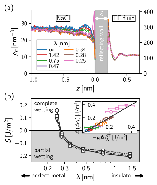
Figure 6: Wetting transition of ionic liquids at metal surfaces. (a) Number density profile $\rho_{n}$ for a molten salt confined between metal surfaces with different screening lengths $\lambda$. The Thomas–Fermi fluid within the metal (right) and the molten salt (left) are separated by a reflective wall of thickness $\xi=0.2$ nm. The average salt density is $\rho_{\mathrm{l}}=27\,\mathrm{nm}^{-3}$. (b) Surface tension difference $\Delta\gamma=\gamma_{\mathrm{gm}}-\gamma_{\mathrm{lm}}$ normalized by the gas/liquid surface tension $\gamma_{\mathrm{gl}}$ as a function of $\lambda$. Symbols indicate different liquid densities $\rho_{\mathrm{l}}$: $27\,\mathrm{nm}^{-3}$ (circles), $25\,\mathrm{nm}^{-3}$ (squares) and $23\,\mathrm{nm}^{-3}$ (triangles). The inset shows the change in the surface tension difference $\Delta(\Delta\gamma(\lambda))$ between an insulator and the Thomas–Fermi fluid at a given $\lambda$. The characteristic length $\ell$ converts the volume energy to a surface energy. Symbols correspond to the same densities as in the main figure, color coding denotes different $\lambda$ as in (a).

Discussion
We developed a classical molecular simulation strategy that allows considering the confinement within any material ranging from perfect metal to insulator. This approach, which does not require to input any given geometry/molecular structure for the confining material, describes in an effective fashion electrostatic screening within confined/vicinal fluids together with the expected capacitive behavior. After straightforward integration into existing simulation packages, this method offers a useful framework to investigate the behavior of dipolar and charged fluids in porous materials made up of any material with imperfect dielectric/metal properties. Beyond practical implications, we also unraveled a non-wetting/wetting crossover in nanoconfined liquids as the confining surfaces vary from insulator to perfect metal. This raises new challenging questions on the complex behavior of charged systems in the vicinity or confined within surfaces with important applications such as electrowetting/switching for energy storage, lubrication, catalysis, etc.

Author contributions

B.C.  L.B. and A.S. conceived the research. A.S. carried out the molecular simulations with support from D.J. A.S., B.C. and L.B. analyzed the data. A.S. and B.C. wrote the paper with inputs from all authors.

Competing Interests

The authors declare no competing interests.

0.1 Molecular Dynamics simulations.

All simulations are carried out using LAMMPS simulation package[48] (stable release 7 Aug 2019). Electrostatic interactions are calculated using the PPPM method with an accuracy of at least $10^{-4}$ and a real-space cut-off $r_{\mathrm{c}}=12.5\,\textrm{\AA}$. Periodic boundary conditions are used in all dimensions with the non-electrostatic interactions being cut and shifted to zero at $r_{\mathrm{c}}$. For the simulations of the TF fluid and the salt in contact with an insulating/vacuum interface, the interactions between periodic images are not screened so that we employ the slab correction method proposed by Yeh and Berkowitz[49] with a vacuum layer of three times the simulation cell height. The non-electrostatic part of the salt–salt interactions are described using the Born–Meyer–Huggins potential which accurately reproduces the properties of NaCl (either as a crystal or molten salt),[41]

$$U_{\mathrm{BMH}}(r)=A\exp\left(\frac{\sigma-r}{B}\right)-\frac{C}{r^{6}}-\frac{D}{r^{8}},$$ (7)

The corresponding force field parameters are given in Supplementary Table 1. Reflective walls of width $\xi=0.2\,\mathrm{nm}$ are used at each metal/dielectric interface to prevent the Thomas–Fermi fluid/charged system to migrate to the pore space/confining media. The latter implies that, if an atom moves through the wall by a distance $\delta$ in a timestep, its position is set back to $-\delta$ away from the wall and the sign of the corresponding velocity component is flipped.

In all simulations presented in the main text, the confining media filled with the Thomas–Fermi fluid are chosen to have a length $d_{\mathrm{TF}}=10\,\mathrm{nm}$. Increasing $d_{\mathrm{TF}}$ increases the agreement between theory and simulations in Fig. 3 due to the decay in the disjoining energy between the two TF surfaces but at the price of enhanced numerical cost (Supplementary Fig. S10). For the TF–TF interaction, a purely repulsive power law of the form $U(r)=E/r^{n}$ is added to avoid numerical infinities when particles overlap. We use $n=8$ and $E=10^{3}\,\textrm{kcal/mol/\AA}^{8}$ but we checked that the detailed form of the interaction potential does not qualitatively influence our simulation results as shown in Supplementary Fig. S9. The positive and negative TF particles differ only in their partial charge $\pm q_{\mathrm{TF}}$ and only interact through electrostatic interactions with the salt. The density of the TF fluid is fixed at $\rho_{\mathrm{TF}}=57.5\,\mathrm{nm^{-3}}$ at a temperature $T_{\mathrm{TF}}=12000\,\mathrm{K}$ and mass $m_{\mathrm{TF}}=1\,\mathrm{amu}$ to ensure fast relaxation. The mass of the Na and Cl atoms is set to 22.9898 and 35.446 amu, respectively. Time integration is performed using a Verlet scheme with a timestep of $0.1\,\mathrm{fs}$ to allow for fast relaxation of the TF liquid. The molten salt is simulated at a 2000 K and temperature coupling is performed using separate Nose–Hoover thermostats for the salt and TF fluids with a characteristic time of 100 timesteps.

0.2 Capacitance determination.

The capacitive behavior of our virtual Thomas–Fermi fluid was checked as this provides an important benchmark to assess its physical validity. Using a direct measurement approach, the capacitance was estimated using MD simulations in which the system is sandwiched between two electrodes having an overall charge $+Q$ and $-Q$. As discussed in the main text, two systems were considered to verify the consistency of the obtained results: the virtual Thomas–Fermi alone and a composite system made up of a dielectric layer confined by the virtual Thomas–Fermi fluid (for the latter, two dielectric materials were considered: either a vacuum layer or a molten salt). The electrodes used for the capacitance measurements consist of point charges $q_{\mathrm{w}}=0.01$ arranged on a 1Å  2D grid (see Supplementary Fig. S2 for a molecular simulation snapshot), resulting in a total charge of $Q=\pm 0.166\,\mathrm{C/m^{2}}$. It was checked that this value is low enough to ensure that the capacitance response of the system is in the linear response regime so that the capcacitance $C$ is readily obtained from the electrostatic potential drop $\Delta\Psi$ between the two electrodes. The TF fluid is separated from the point charges by 1Å via a reflecting wall denoted by the gray shaded areas in Fig. 4(a). The potential drop is obtained from Poisson equation by integrating twice the charge density profile, $\Delta\Psi(z)=-\int_{-\infty}^{z}{\mathrm{d}}z^{\prime}\int_{-\infty}^{z\prime}{\mathrm{d}}z^{\prime\prime}\,e(\rho_{+}-\rho_{-})/\varepsilon_{0}$ as shown in Supplementary Fig. S2(b).

Data availability

All relevant simulation input scripts are available in this repository: Schlaich, Alexander, 2021, ”Simulation input scripts for ’Electronic screening using a virtual Thomas–Fermi fluid for predicting wetting and phase transitions of ionic liquids at metal surfaces’”, https://doi.org/10.18419/darus-2115, DaRUS.

Code availability

Molecular simulations were performed using using the open source package LAMMPS, stable release 7 Aug 2019, available under https://www.lammps.org/. Post-processing has been performed in Python using our open source toolbox MAICoS (https://gitlab.com/maicos-devel/maicos/).

in 1,…,0 See pages \x of TF_supplement.pdf

References

- [1] Bocquet, L. & Charlaix, E. Nanofluidics, from bulk to interfaces. Chem. Soc. Rev. 39, 1073–1095 (2010).
- [2] Schoch, R. B., Han, J. & Renaud, P. Transport phenomena in nanofluidics. Rev. Mod. Phys. 80, 839–883 (2008).
- [3] Bazant, M. Z., Storey, B. D. & Kornyshev, A. A. Double Layer in Ionic Liquids: Overscreening versus Crowding. Phys. Rev. Lett. 106, 046102 (2011).
- [4] Smith, A. M., Lee, A. A. & Perkin, S. The Electrostatic Screening Length in Concentrated Electrolytes Increases with Concentration. J. Phys. Chem. Lett. 7, 2157–2163 (2016).
- [5] Lainé, A., Niguès, A., Bocquet, L. & Siria, A. Nanotribology of Ionic Liquids: Transition to Yielding Response in Nanometric Confinement with Metallic Surfaces. Phys. Rev. X 10, 011068 (2020).
- [6] Fedorov, M. V. & Kornyshev, A. A. Ionic Liquids at Electrified Interfaces. Chem. Rev. 114, 2978–3036 (2014).
- [7] Kaiser, V. et al. Electrostatic interactions between ions near Thomas–Fermi substrates and the surface energy of ionic crystals at imperfect metals. Faraday Discuss. 199, 129–158 (2017).
- [8] Dufils, T., Scalfi, L., Rotenberg, B. & Salanne, M. A semiclassical Thomas-Fermi model to tune the metallicity of electrodes in molecular simulations. arXiv:1910.13341 [cond-mat] (2019). 1910.13341.
- [9] Newns, D. M. Fermi–Thomas Response of a Metal Surface to an External Point Charge. J. Chem. Phys. 50, 4572–4575 (1969).
- [10] Inkson, J. C. Many-body effect at metal-semiconductor junctions. II. The self energy and band structure distortion. J. Phys. C: Solid State Phys. 6, 1350–1362 (1973).
- [11] Kornyshev, A. A., Rubinshtein, A. I. & Vorotyntsev, M. A. Image potential near a dielectric–plasma-like medium interface. physica status solidi (b) 84, 125–132 (1977).
- [12] Luque, N. B. & Schmickler, W. The electric double layer on graphite. Electrochimica Acta 71, 82–85 (2012).
- [13] Kornyshev, A. A., Luque, N. B. & Schmickler, W. Differential capacitance of ionic liquid interface with graphite: The story of two double layers. J Solid State Electrochem 18, 1345–1349 (2014).
- [14] Netz, R. R. Debye-Hückel theory for interfacial geometries. Phys. Rev. E 60, 3174–3182 (1999).
- [15] Lee, A. A. & Perkin, S. Ion–Image Interactions and Phase Transition at Electrolyte–Metal Interfaces. J. Phys. Chem. Lett. 7, 2753–2757 (2016).
- [16] Bedrov, D. et al. Molecular Dynamics Simulations of Ionic Liquids and Electrolytes Using Polarizable Force Fields. Chem. Rev. 119, 7940–7995 (2019).
- [17] Breitsprecher, K., Szuttor, K. & Holm, C. Electrode Models for Ionic Liquid-Based Capacitors. J. Phys. Chem. C 119, 22445–22451 (2015).
- [18] Comtet, J. et al. Nanoscale capillary freezing of ionic liquids confined between metallic interfaces and the role of electronic screening. Nature Materials 16, 634–639 (2017).
- [19] Ashcroft, N. W. & Mermin, N. D. Solid State Physics (Holt, Rinehart and Winston, 1976).
- [20] dos Santos, A. P., Girotto, M. & Levin, Y. Simulations of Coulomb systems confined by polarizable surfaces using periodic Green functions. J. Chem. Phys. 147, 184105 (2017).
- [21] Siepmann, J. I. & Sprik, M. Influence of surface topology and electrostatic potential on water/electrode systems. J. Chem. Phys. 102, 511–524 (1995).
- [22] Reed, S. K., Lanning, O. J. & Madden, P. A. Electrochemical interface between an ionic liquid and a model metallic electrode. The Journal of Chemical Physics 126, 084704 (2007).
- [23] Tyagi, S. et al. An iterative, fast, linear-scaling method for computing induced charges on arbitrary dielectric boundaries. J. Chem. Phys. 132, 154112 (2010).
- [24] Arnold, A. et al. Efficient Algorithms for Electrostatic Interactions Including Dielectric Contrasts. Entropy 15, 4569–4588 (2013).
- [25] Nguyen, T. D., Li, H., Bagchi, D., Solis, F. J. & Olvera de la Cruz, M. Incorporating surface polarization effects into large-scale coarse-grained Molecular Dynamics simulation. Computer Physics Communications 241, 80–91 (2019).
- [26] Torrie, G. M. & Valleau, J. P. Double layer structure at the interface between two immiscible electrolyte solutions. Journal of Electroanalytical Chemistry and Interfacial Electrochemistry 206, 69–79 (1986).
- [27] Kornyshev, A. A. & Vorotyntsev, M. A. Nonlocal electrostatic approach to the double layer and adsorption at the electrode-electrolyte interface. Surface Science 101, 23–48 (1980).
- [28] Vorotyntsev, M. A. Modern State of Double Layer Study of Solid Metals. In Bockris, J. O., Conway, B. E. & White, R. E. (eds.) Modern Aspects of Electrochemistry: Volume 17, Modern Aspects of Electrochemistry, 131–222 (Springer US, Boston, MA, 1986).
- [29] Kornyshev, A. A. & Vorotyntsev, M. A. Electrostatic Interaction at the metal/dielectric interface. Sov. Phys. JETP 51, 509–513 (1980).
- [30] Vorotyntsev, M. A. No. Part C in The Chemical Physics of Solvation, 401 (Elsevier, Amsterdam, 1988).
- [31] Kornyshev, A. A. & Schmickler, W. On the coverage dependence of the partial charge transfer coefficient. Journal of Electroanalytical Chemistry and Interfacial Electrochemistry 202, 1–21 (1986).
- [32] Vorotyntsev, M., Kornyshev, A. & Rubinshtein, A. Possible Mechanisms of Controlling Ionic Interaction at the Electrode-Solution Interface. Soviet Electrochemistry 16, 65–67 (1980).
- [33] Kornyshev, A. A. Metal electrons in the double layer theory. Electrochimica Acta 34, 1829–1847 (1989).
- [34] Gerischer, H. An interpretation of the double layer capacity of graphite electrodes in relation to the density of states at the Fermi level. J. Phys. Chem. 89, 4249–4251 (1985).
- [35] Gerischer, H., McIntyre, R., Scherson, D. & Storck, W. Density of the electronic states of graphite: Derivation from differential capacitance measurements. J. Phys. Chem. 91, 1930–1935 (1987).
- [36] Kondrat, S. & Kornyshev, A. Superionic state in double-layer capacitors with nanoporous electrodes. J. Phys.: Condens. Matter 23, 022201 (2010).
- [37] Li, Z., Mendez-Morales, T. & Salanne, M. Computer simulation studies of nanoporous carbon-based electrochemical capacitors. Current Opinion in Electrochemistry 9, 81–86 (2018).
- [38] Rochester, C. C., Lee, A. A., Pruessner, G. & Kornyshev, A. A. Interionic Interactions in Conducting Nanoconfinement. ChemPhysChem 14, 4121–4125 (2013).
- [39] Mohammadzadeh, L. et al. On the Energetics of Ions in Carbon and Gold Nanotubes. ChemPhysChem 17, 78–85 (2016).
- [40] Bi, S. et al. Minimizing the electrosorption of water from humid ionic liquids on electrodes. Nature Communications 9, 5222 (2018).
- [41] Anwar, J., Frenkel, D. & Noro, M. G. Calculation of the melting point of NaCl by molecular simulation. J. Chem. Phys. 118, 728–735 (2002).
- [42] Nijmeijer, M. J. P., Bruin, C., Bakker, A. F. & van Leeuwen, J. M. J. Wetting and drying of an inert wall by a fluid in a molecular-dynamics simulation. Phys. Rev. A 42, 6052–6059 (1990).
- [43] de Gennes, P. G. Wetting: Statics and dynamics. Rev. Mod. Phys. 57, 827–863 (1985).
- [44] Rowlinson, J. S. & Widom, B. Molecular Theory of Capillarity (Courier Corporation, 1982).
- [45] Bonn, D., Eggers, J., Indekeu, J., Meunier, J. & Rolley, E. Wetting and spreading. Rev. Mod. Phys. 81, 739–805 (2009).
- [46] Evans, R., Stewart, M. C. & Wilding, N. B. A unified description of hydrophilic and superhydrophobic surfaces in terms of the wetting and drying transitions of liquids. PNAS 116, 23901–23908 (2019).
- [47] Damaskin, B. Adsorption of Organic Compounds on Electrodes (Springer, Boston, MA, 2012), softcover reprint of the original 1st ed. 1971 edition edn.
- [48] Plimpton, S. Fast Parallel Algorithms for Short-Range Molecular Dynamics. J. Comput. Phys. 117, 1–19 (1995).
- [49] Yeh, I.-C. & Berkowitz, M. L. Ewald summation for systems with slab geometry. The Journal of Chemical Physics 111, 3155–3162 (1999).