A Comparative Study of Machine Learning Models for Predicting the State of Reactive Mixing

Abstract

Mixing phenomena are important mechanisms controlling flow, species transport, and reaction processes in fluids and porous media. Accurate predictions of reactive mixing are critical for many Earth and environmental science problems such as contaminant fate and remediation, macroalgae growth, and plankton biomass evolution. To investigate mixing dynamics over time under different scenarios (e.g., anisotropy, fluctuating velocity fields), a high-fidelity, finite-element-based numerical model is built to solve the fast, irreversible bimolecular reaction-diffusion equations to simulate a range of reactive-mixing scenarios. A total of 2,315 simulations are performed using different sets of model input parameters comprising various spatial scales of vortex structures in the velocity field, time-scales associated with velocity oscillations, the perturbation parameter for the vortex-based velocity, anisotropic dispersion contrast (i.e., ratio of longitudinal-to-transverse dispersion), and molecular diffusion. Outputs comprise concentration profiles of the reactants and products. The inputs and outputs of these simulations are concatenated into feature and label matrices, respectively, to train 20 different machine learning (ML) emulators to approximate system behavior. The 20 ML emulators based on linear methods, Bayesian methods, ensemble learning methods, and multilayer perceptron (MLP), are compared to assess these models. The ML emulators are specifically trained to classify the state of mixing and predict three quantities of interest (QoIs) characterizing species production, decay (i.e., average concentration, square of average concentration), and degree of mixing (i.e., variances of species concentration). Linear classifiers and regressors fail to reproduce the QoIs; however, ensemble methods (classifiers and regressors) and the MLP accurately classify the state of reactive mixing and the QoIs. Among ensemble methods, random forest and decision-tree-based AdaBoost faithfully predict the QoIs. At run time, trained ML emulators are $\approx 10^{5}$ times faster than the high-fidelity numerical simulations. Speed and accuracy of the ensemble and MLP models facilitate uncertainty quantification, which usually requires 1,000s of model run, to estimate the uncertainty bounds on the QoIs.

Keywords: Surrogate modeling, machine learning, reaction-diffusion equations, random forests, ensemble methods, artificial neural networks.

1   Introduction

Reactive-mixing phenomena dictate the distribution of chemical species in fluids (e.g., coastal waters) and subsurface porous media. Accurate quantification of species concentration is critical to remediation applications such as nuclear remediation, spill distribution, algal-bloom forecasting, etc [1, 2, 3, 4, 5, 6, 7, 8, 9, 10]. Parameters that influence reactive-mixing in fluids and subsurface porous media include the structure of the flow field (e.g., chaotic advection), fluid injection/extraction (i.e., location of wells, injection/extraction rates), subsurface heterogeneity, dispersion, and anisotropy [11, 12]. These parameters have variable impacts on important quantities of interest (QoIs) such as species production and decay (e.g., average and squared average species concentrations) and degree of mixing (i.e., variances of species concentrations). For QoIs, nonlinear partial differential equations are solved using high-fidelity numerical methods (e.g., finite-difference, -element,or -volume methods) that can take hours to days (for $\approx\mathcal{O}(10^{6})-\mathcal{O}(10^{9})$ degrees-of-freedom) on state-of-the-art, high-performance computing (HPC) machines. Such computation times preclude real-time predictions, which can be critical to decision making for remediation activities. Hence, alternative faster approaches are needed and machine learning (ML)-based emulators show promise [13, 14, 15, 16, 17]. Here, we build and compare various ML emulators to predict reactive-mixing QoIs. The ML emulators are trained and tested using data from high-fidelity, finite-element numerical simulations, which expressly reflect the underlying reaction-diffusion physics in anisotropic porous media.

Given sufficient data, ML models can successfully detect, quantify, and predict different types of phenomena in the geosciences [18, 19]. Applications include remote sensing [17, 20], ocean wave forecasting [21, 22, 23], seismology [24, 25, 13, 26, 14, 27], hydrogeology [28, 16, 15], and geochemistry [29, 30, 31, 32, 33]. ML emulators (also known as surrogate models or reduced-order models) can be fast, reliable, and robust when trained on large datasets [19, 18, 34]. ML emulators are constructed using training data (e.g., features and labels), which include inputs and outputs either from field data, experimental data, high-fidelity numerical simulations, or any combination of these [34, 35]. In this paper, we compare emulators based on generalized linear methods [36, 37], Bayesian methods [38, 39], ensemble methods [40, 41], and an MLP [42, 42, 43] to predict various QoIs.

Previous researchers have used unsupervised and supervised ML methods to reproduce reactive-mixing QoIs. Vesselinov et al. [11] used non-negative tensor factorization with custom $k$-means clustering (unsupervised ML) to identify hidden features in the solutions to reaction-diffusion equations. They determined that anisotropy features (i.e., longitudinal and transverse dispersion) govern reactive mixing at early to middle times while molecular diffusion controls product formation at late times. They also quantified the effects of longitudinal and transverse dispersion and molecular diffusion on species production and decay over time. Mudunuru and Karra [12] ranked the importance of input parameters/features on reactive-mixing QoIs. Also, they developed support vector machine (SVM) and support vector regressor (SVR) emulators to classify the degree of mixing and to predict QoIs. However, SVM/SVR training times increase significantly with the size of the training data set [12]. To obviate this problem, in the present paper, we build ML emulators whose training times are $\approx 10^{5}$ times faster than SVM and SVR without compromising accuracy.

Specifically, we compare one linear classifier, two Bayesian classifiers, an ensemble classifier, an MLP classifier, seven linear regressors, six ensemble regressors, and an MLP regressor. Emulator performance is assessed according to training and testing scores, training time, and $R^{2}$ score on the QoIs from a blind data set. The blind data set includes six realizations that are not seen during training and testing phases. This study addresses the following questions: (1) Can ML emulators accurately classify the mixing state of the anisotropic reaction-diffusion system? (2) How accurately do they predict QoIs of reactive mixing? (3) How fast can they be trained? (4) How does each emulator rank overall?

2   Governing Equations for Reactive Mixing

Let $\Omega\subset{\rm I\!R}^{d}$ be an open bounded domain, where $d$ indicates the number of spatial dimensions. The boundary is denoted by $\partial\Omega$, which is assumed to be piece-wise smooth. Let $\overline{\Omega}$ be the set closure of $\Omega$ and let spatial point $\mathbf{x}\in\overline{\Omega}$. The divergence and gradient operators with respect to $\mathbf{x}$ are denoted by $\mathrm{div}[\bullet]$ and $\mathrm{grad}[\bullet]$, respectively. Let $\mathbf{n}(\mathbf{x})$ be the unit outward normal to $\partial\Omega$. Let $t\in\,]0,\mathcal{I}[$ denote time, where $\mathcal{I}$ is the length of time of interest. The governing equations are posed on $\Omega\times]0,\mathcal{I}[$ and the initial condition is specified on $\overline{\Omega}$. Consider the fast bimolecular reaction where species $A$ and $B$ react irreversibly to yield product $C$:

$$n_{A}\,A\,+\,n_{B}\,B\longrightarrow n_{C}\,C.$$ (1)

The governing equations for this fast bimolecular reaction without volumetric sources/sinks are:

$$\frac{\partial c_{A}}{\partial t}-\mathrm{div}[\mathbf{D}(\mathbf{x},t)\,\mathrm{grad}[c_{A}]]=-n_{\small{A}}\,k_{AB}c_{A}c_{B}\quad\mathrm{in}\;\Omega\times]0,\mathcal{I}[,$$ (2a)

$$\frac{\partial c_{B}}{\partial t}-\mathrm{div}[\mathbf{D}(\mathbf{x},t)\,\mathrm{grad}[c_{B}]]=-n_{\small{B}}\,k_{AB}c_{A}c_{B}\quad\mathrm{in}\;\Omega\times]0,\mathcal{I}[,$$ (2b)

$$\frac{\partial c_{C}}{\partial t}-\mathrm{div}[\mathbf{D}(\mathbf{x},t)\,\mathrm{grad}[c_{C}]]=+n_{\small{C}}\,k_{AB}c_{A}c_{B}\quad\mathrm{in}\;\Omega\times]0,\mathcal{I}[,$$ (2c)

$$c_{i}(\mathbf{x},t)=c^{\mathrm{p}}_{i}(\mathbf{x},t)\quad\mathrm{on}\;\Gamma^{\mathrm{D}}_{i}\times]0,\mathcal{I}[\quad(i=A,\,B,\,C),$$ (2d)

$$\left(-\mathbf{D}(\mathbf{x},t)\,\mathrm{grad}[c_{i}]\right)\cdot\mathbf{n}(\mathbf{x})=h^{\mathrm{p}}_{i}(\mathbf{x},t)\quad\mathrm{on}\;\Gamma^{\mathrm{N}}_{i}\times]0,\mathcal{I}[\quad(i=A,\,B,\,C),$$ (2e)

$$c_{i}(\mathbf{x},t=0)=c^{0}_{i}(\mathbf{x})\quad\mathrm{in}\;\overline{\Omega}\quad(i=A,\,B,\,C).$$ (2f)

Traditional numerical formulations for Eqs. (2a)–(2f) can yield nonphysical solutions for chemical species concentration [44]. Also, when anisotropy dominates, the standard Galerkin formulation produces erroneous concentrations [45, 46, 47, 44]. To overcome these problems, a non-negative, finite-element method is used to compute species concentrations [44]. This method ensures that concentrations are non-negative and satisfy the discrete maximum principle.

2.1   Reaction Tank Problem and Associated QoIs

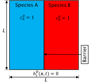
Figure 1. Model domain for reactive-mixing: Schematic of the initial boundary value problem. $L$, $h_{i}^{\mathrm{p}}\left(\mathbf{x},t\right)$, $c_{A}^{0}$, and $c_{B}^{0}$ are the length of the domain, diffusive flux on the boundary for $i^{\mathrm{th}}$ chemical species, initial concentration of species $A$, and initial concentration of species $B$, respectively. Species $A$ and $B$ were initially on the left and right sides of the domain, respectively. Initial concentrations of $A$ and $B$ were 1.0 and mixing commenced for $t>0$.

Figure 1 depicts the initial boundary-value problem. The model domain is a square with $L=1$. Zero-flux boundary conditions $h_{i}^{\mathrm{p}}\left(\mathbf{x},t\right)=0$ are enforced on all sides of the domain. For all chemical species, the non-reactive volumetric source $f_{i}(\mathbf{x},t)$ is equal to zero. Initially, species $A$ and $B$ are segregated (see Fig. 1) and stoichiometric coefficients are $n_{A}=1$, $n_{B}=1$, and $n_{C}=1$. The total time of interest is $\mathcal{I}=1$. The dispersion tensor is taken from the subsurface literature [48, 44]:

$$\mathbf{D}_{\mathrm{subsurface}}(\mathbf{x})=D_{\mathrm{m}}\mathbf{I}+\alpha_{\mathrm{T}}\|\mathbf{v}\|\mathbf{I}+\frac{\alpha_{\mathrm{L}}-\alpha_{\mathrm{T}}}{\|\mathbf{v}\|}\mathbf{v}\otimes\mathbf{v}.$$ (3)

The model velocity field is used to define the dispersion tensor according to stream function [49, 50, 51]:

$$\psi(\mathbf{x},t)=\begin{cases}\frac{1}{2\pi\kappa_{\mathrm{f}}}\left[\sin(2\pi\kappa_{\mathrm{f}}x)-\sin(2\pi\kappa_{\mathrm{f}}y)+v_{0}\cos(2\pi\kappa_{\mathrm{f}}y)\right]&\;\;\mathrm{if}\;\nu T\leq t<\left(\nu+\frac{1}{2}\right)T\\ \frac{1}{2\pi\kappa_{\mathrm{f}}}\left[\sin(2\pi\kappa_{\mathrm{f}}x)-\sin(2\pi\kappa_{\mathrm{f}}y)-v_{0}\cos(2\pi\kappa_{\mathrm{f}}x)\right]&\;\;\mathrm{if}\;\left(\nu+\frac{1}{2}\right)T\leq t<\left(\nu+1\right)T\end{cases}.$$ (4)

Using Eq. (4), the divergence-free velocity field components are:

$$\mathrm{v}_{x}(\mathbf{x},t)=-\frac{\partial\psi}{\partial\mathrm{y}}=\begin{cases}\cos(2\pi\kappa_{\mathrm{f}}y)+v_{0}\sin(2\pi\kappa_{\mathrm{f}}y)&\quad\mathrm{if}\;\nu T\leq t<\left(\nu+\frac{1}{2}\right)T\\ \cos(2\pi\kappa_{\mathrm{f}}y)&\quad\mathrm{if}\;\left(\nu+\frac{1}{2}\right)T\leq t<\left(\nu+1\right)T\end{cases},$$ (5)

$$\mathrm{v}_{y}(\mathbf{x},t)=+\frac{\partial\psi}{\partial\mathrm{x}}=\begin{cases}\cos(2\pi\kappa_{\mathrm{f}}x)&\quad\mathrm{if}\;\nu T\leq t<\left(\nu+\frac{1}{2}\right)T\\ \cos(2\pi\kappa_{\mathrm{f}}x)+v_{0}\sin(2\pi\kappa_{\mathrm{f}}x)&\quad\mathrm{if}\;\left(\nu+\frac{1}{2}\right)T\leq t<\left(\nu+1\right)T\end{cases}.$$ (6)

In Eqs. (5)–(6), $T$ controls the oscillation of the velocity field from clockwise to anti-clockwise. $v_{0}$ is the perturbation parameter of the underlying vortex-based flow field. Larger values of $v_{0}$ skew the vortices into ellipses while smaller values of $v_{0}$ yield circular vortex structures in the velocity field. $\frac{\alpha_{\mathrm{L}}}{\alpha_{\mathrm{T}}}$ controls the magnitude of the anisotropic dispersion contrast. Smaller values of $\frac{\alpha_{\mathrm{L}}}{\alpha_{\mathrm{T}}}$ indicate less anisotropy and vice versa. The magnitude of $\kappa_{\mathrm{f}}L$ governs the size of the vortex structures in the flow field [11, 12]. Note that varying $v_{0}$ does not significantly alter vortex locations.

For reactive-mixing applications, the following QoIs are defined:

1. Species production/decay, which can be analyzed by calculating normalized average concentrations, $\overline{c}_{i}$, and normalized average of squared concentrations, $\overline{c^{2}}_{i}$. Normalized average of squared concentration, $\overline{c^{2}}_{i}$, provides information on the species production/decay as a function of the eigenvalues of anisotropic dispersion. For example, see Theorem 2.3 in Reference [12], which shows that $\overline{c^{2}}_{i}$ is bounded above and below by an exponential function of minimum and maximum eigenvalues of anisotropic dispersion. These quantities are:

   $$\overline{c}_{i} :=\frac{\langle c_{i}(t)\rangle}{\mathrm{max}\left[\langle c_{i}(t)\rangle\right]}\quad\mathrm{where}\;\left\langle c_{i}(t)\right\rangle=\int\limits_{\Omega}c_{i}(\mathbf{x},t)\,\mathrm{d}\Omega,$$ (7)

   $$\overline{c^{2}}_{i} :=\frac{\langle c^{2}_{i}\rangle}{\mathrm{max}\left[\langle c^{2}_{i}\rangle\right]}\quad\mathrm{where}\;\left\langle c^{2}_{i}(t)\right\rangle=\int\limits_{\Omega}c^{2}_{i}(\mathbf{x},t)\,\mathrm{d}\Omega.$$ (8)

2. Degree of mixing is defined as the variance of concentration:

   $$\sigma^{2}_{c_{i}}:=\frac{\langle c^{2}_{i}\rangle-\langle c_{i}\rangle^{2}}{\mathrm{max}\left[\langle c^{2}_{i}\rangle-\langle c_{i}\rangle^{2}\right]}.$$ (9)

Note that the values for $\overline{c}_{i}$, $\overline{c^{2}}_{i}$, and $\sigma^{2}_{c_{i}}$ are non-negative and range from 0 to 1 $\forall\quad i=A,B,C$.

2.2   Feature Generation (Numerical Model Inputs)

First, a 2D numerical model is built using first-order finite-element structured triangular mesh, which has 81 nodes on each side. A total of 2,500 high-fidelity numerical simulations are run for different sets of reaction-diffusion model input parameters, of which 2,315 run to completion because certain parameter combinations do not yield to stable solution. Each simulation run uses 1,000 time steps ($\mathcal{I}=$ $0.0$ to $1.0$ with a uniform time step of $0.001$). Features include: longitudinal-to-transverse anisotropic dispersion ratio $\frac{\alpha_{\mathrm{L}}}{\alpha_{\mathrm{T}}}$, molecular diffusion $D_{\mathrm{m}}$, the perturbation parameter of the underlying vortex-based velocity field $v_{0}$, and velocity field characteristics scales $\kappa_{\mathrm{f}}L$ and $T$. Specifically, input parameters are: $v_{0}=\left[1,10^{-1},10^{-2},10^{-3},10^{-4}\right]$, $\frac{\alpha_{\mathrm{L}}}{\alpha_{\mathrm{T}}}=\left[1,10^{1},10^{2},10^{3},10^{4}\right]$, $D_{m}=\left[10^{-8},10^{-3},10^{-2},10^{-1}\right]$, $\kappa_{\mathrm{f}}L$ = $\left[1,2,3,4,5\right]$, and $T=[1\times 10^{-4},~{}2\times 10^{-4},3\times 10^{-4},4\times 10^{-4},5\times 10^{-4}]$. $\alpha_{\mathrm{T}}$ is varied with $\alpha_{\mathrm{L}}$ held at 1.0. Five features for each of the 2,315 models with 1,000 time steps formed the feature matrix with dimensions $2,315,000\times 5$.

3   Machine Learning Emulators

3.1   Labels (QoIs) and Preprocessing

Labels are the QoIs of the 2,315 simulations at each time step yielding label vectors. Features and labels are concatenated into training and testing data forming a $2,315,000\times 6$ matrix. For ML classification, the degree of mixing in the system is characterized by four classes representing: Class-1 (well mixed), Class-2 (moderately mixed), Class-3 (weakly mixed), and Class-4 (ultra-weak mixing). The corresponding $\sigma^{2}_{i}$ for these classes are 0.0–0.25, 0.25–0.5, 0.5–0.75, and 0.75–1.0, respectively. Of course, additional classes could be defined although this would necessitate re-training of ML emulators. These data are partitioned into training and testing data during construction of the ML emulators and Table 1 lists the different partitions. Each emulator is trained using the three different data partitions and the performance of each assessed. First, 0.9% of data are used as training data to identify optimized hyperparameters and other tunable parameters. Subsequently, emulators using the optimized hyperparameters are validated against 63% and 81% of data partitions.

Preprocessing is typically required for ML emulator development. ML emulators that use the Euclidean norm (e.g., kernel-based methods) must have all features/input parameters of the same scale to make accurate predictions [52, 53, 54]. Common preprocessors are standardization (recasting all feature data into the standard normal distribution $N(0,1)$), normalization (independently scaling each feature between $0$ and $1$), and max-abs scaling (scale and translate individual features such that the maximal absolute value of a feature is 1). In this study, except for Random Forests (RF), which is agnostic to feature scaling, because features are neither sparse nor skewed and do not have outliers, all data are standardized. For polynomial regression, we use the quadratic transformation of the data.

3.2   Optimization of Hyperparameter and Other Tunable Parameters

Every ML emulator learns a function or a set of functions by comparing features and corresponding labels. During this process, different hyperparameters for each ML emulator control the learning process. Some common hyperparameters are regularization, learning rate, and the cost function. In addition, there are additional tunable parameters for each ML emulator that also speed the learning process and make a more robust emulator, including the number of training iterations, kernel, truncation value, etc. Because hyperparameter optimization is an exhaustive, time-consuming process, 0.9% of the data (23 simulations) were used with the Gridsearch algorithm in Scikit-learn [55], a Python ML package. Tables 4 and 5 list the hyperparameters for each ML emulator. Later, 7% and 9% of the data were used for validation with 30% or 10% reserved as blind data for testing.

Because, ML emulators can introduce bias during training, overfitting is a common phenomenon. To ameliorate this, $k$-fold cross-validation algorithm is used to avoid bias, to determine optimal computational times, and to calculate reliable variances [56, 57]. In this work, 10-fold cross-validation is used [56, 57]. First, it subdivides training data into equal ten subsets. Then, it uses nine sets for training while one set is left for validation, and this process is repeated leaving out each subset once. The average performance on the 10 withheld data sets are reported along with their variance.

Table 1. Summary of training and testing data partitions used in ML emulator development and testing.

% of input data (No. of simulations)			Size of samples for QoIs
Training data	Validation data	Testing data	Training	Testing
0.9% (20)	0.1 (3) %	99% (2,292)	20,150	2,291,850
63% (1458)	7% (162)	30% (690)	1,458,500	694,500
81% (1875)	9% (208)	10% (230)	1,875,500	231,500

3.3   ML Emulators

This research applies 20 ML emulators to classify the state of reactive mixing and to predict the reactive-mixing QoIs. Among the 20 ML emulators, eight are linear, five are Bayesian, six are ensemble, and one is an MLP. The eight linear ML emulators are ordinary least square regressor (LSQR), ridge regressor (RR), lasso regressor (LR), elastic-net regressor (ER), Huber regressor (HR), polynomial, logistic regression (LogR), and kernel ridge (KR). Among the linear emulators, only LogR is a classifier. The five Bayesian techniques are – Bayesian ridge (BR), Gaussian process (GP), naïve Bayes (NB), linear discriminant analysis (LDA), and quadratic discriminant analysis (QDA). Among these Bayesian emulators, LDA and QDA are classifiers and remaining are regressors. The six ensemble ML emulators are bagging, decision tree (DT), random forest (RF), AdaBoost (AdaB), DT-based AdaB, and gradient boosting method (GBM). Among the six ensemble emulators, RF is used as both classifier and regressor. MLP is also used as both classifier and regressor.

3.4   Linear ML Emulators

Linear ML emulators tend to fit a straight line to the labels. Each linear emulators’ equation is listed in Table 2 along with its corresponding cost function. A brief mathematical description of each linear ML emulator is explained at Appendix A. The equation for polynomial regression is not listed here because it applies the LSQR formula to quadratic-scaled data. For LSQR and polynomial regressor, we optimize intercept. For RR, $\alpha_{2}$ and $\epsilon$ (tolerance/threshold) are optimized. For LR, $\alpha_{1}$, $\epsilon$, and maximum iteration number are optimized. For ER, $\alpha_{1}$, $\alpha_{2}$, $\epsilon$, $l_{\mathrm{1}}$ ratio, and maximum iteration number are optimized. For HR, $\alpha_{1}$, $\epsilon$, and maximum iteration number are optimized. Optimized hyperparameters and other tunable parameters (bolded) for linear ML emulators are listed in Table 4. For Logistic regression, multi-class (binary or multi-class), solver, $\epsilon$, and maximum number of iterations are optimized and corresponding settings are presented in Table 4. Tested solvers include Newton’s method, limited memory large-scale bound constrained (LBFGS) solver, and the stochastic average gradient (SAG) solver. For KR, $\alpha_{1}$, $\lambda$, and kernels are optimized (see, Table 4).

Table 2. Equation and cost function of linear emulators.

Emulator	Equation	Cost function
LSQR	$\hat{y}\left(\mathbb{w},\mathbb{x}\right)=w_{0}+w_{1}x_{1}+\cdots+w_{n}x_{n}=\mathbb{x}\cdot\mathbb{w}$	$L_{\mathrm{lsqr}}=\underset{\mathbb{w}}{\mathrm{min}}||\mathbb{X}\mathbb{w}-\mathbb{y}||_{2}^{2}$
RR	Same as above	$L_{\mathrm{RR}}=\underset{\mathbb{w}}{\mathrm{min}}||\mathbb{X}\mathbb{w}-\mathbb{y}||_{2}^{2}+\alpha_{2}||\mathbb{w}||_{2}^{2}$
LR	Same as above	$L_{\mathrm{LR}}=\underset{\mathbb{w}}{\mathrm{min}}||\mathbb{X}\mathbb{w}-\mathbb{y}||_{2}^{2}+\alpha_{1}||\mathbb{w}||_{1}$
ER	Same as above	$L_{\mathrm{ER}}=\underset{\mathbb{w}}{\mathrm{min}}||\mathbb{X}\mathbb{w}-\mathbb{y}||_{2}^{2}+\alpha_{1}||\mathbb{w}||_{1}+\alpha_{2}||\mathbb{w}||_{2}^{2}$
HR	Same as above	$L_{\mathrm{HR}}=\underset{\mathbb{w}}{\mathrm{min}}||\mathbb{X}\mathbb{w}-\mathbb{y}||_{2}^{2}+\alpha_{1}||\mathbb{w}||_{1}+\Sigma\sum_{i=1}^{m}\left[1+H_{\epsilon}\left(\frac{\mathbb{x}_{i}\cdot\mathbb{w}-y_{i}}{\Sigma}\right)\right]$
LogR	$l=\log_{\mathrm{b}}\left(\frac{p}{1-p}\right)=w_{0}+w_{1}x_{1}+w_{2}x_{2}$	$L_{\mathrm{cross-entropy}}=-\frac{1}{n}\sum_{n=1}^{n}\left[y_{n}\log\left(p_{n}\right)+\left(1-y_{n}\right)\log\left(1-p_{n}\right)\right]$
KR	$\mathcal{K}_{\mathrm{RBF}}\left(\mathbb{x_{1}},\mathbb{x_{2}}\right)=\mathrm{exp}\left(-\lambda\left|\left|\mathbb{x_{1}}-\mathbb{x_{2}}\right|\right|^{2}\right)$	$L_{\mathrm{squared}}=\left(y-\hat{y}\right)^{2}$

3.5   Bayesian ML Emulators

Bayesian ML emulators apply Bayes’ rule to learn function from labels to predict equivalent label. Equations for Bayesian ML emulators are listed in Table 3. Also, a brief mathematical description of each Bayesian ML emulator is explained in Appendix A. For BR, $\beta$, $\mathrm{\omega}$, maximum iterations, and $\epsilon$ are the hyperparameters and their optimized values are shown in bold in Table 5. For GP, kernel is optimized and its best is listed in Table 5. In NB, only priors and variance smoothing are hyperparameters. For LDA, solver is optimized; solvers include singular value decomposition (SVD), LSQR, eigen value decomposition. Among these three, SVD is fastest. For QDA, only tolerance is optimized and best value is $10^{-4}$.

3.6   Ensemble Emulators

If the relationship between features and label is nonlinear, linear ML emulators are not expected to perform well. Instead, nonlinear ML emulators such as an MLP and ensemble methods should work better. Ensemble methods bootstrap (random sampling with replacement) data to develop different tree models/predictors. Each label is used with replacement as input for developing individual models; therefore, tree models have different labels based on the bootstrap process. Because bootstrapping captures many uncorrelated base learners to develop a final model, it reduces variance; resulting in a reduced prediction error. Also, in ensemble models, many different trees predict the same target variable; therefore, they predict better than any single tree alone.

Ensemble techniques are further classified into Bagging (bootstrapping aggregating) and Boosting (form many weak trees/learners into a strong tree). While bagging emulators work best with strong and complex trees (e.g., fully developed decision trees), boosting emulators work best with weak models (e.g., shallow decision trees). In this study, several averaging/bagging and boosting ensemble emulators are explored to classify and predict reactive mixing. The averaging emulators include bagging and RF while boosting emulators include AdaBoost (AdaB), DT-based AdaB, and gradient boosting method (GBM).

Table 3. Equation and cost function of Bayesian, ensemble, and MLP emulators where $L_{\mathrm{lml}}=-\frac{1}{2}\left(\log\|\omega^{-1}\mathbb{I}+\mathbf{\Phi}\mathbf{A}^{-1}\mathbf{\Phi}^{\intercal}\|+\mathbf{\Psi}^{\intercal}\left(\mathrm{\omega}^{-1}\mathbb{I}+\mathbf{\Phi}\mathbf{A}^{-1}\mathbf{\Phi}^{\intercal}\right)^{-1}\mathbf{\Psi}\right)+\sum_{i=0}^{N}\left(o\log\beta_{i}-\mathrm{r}\beta_{i}\right)+u\log\omega-w\omega$.

Emulator	Equation	Cost function
BR	$p\left(\mathbb{w}|\mathrm{\omega}\right)=N\left(\mathbb{w}|0,\mathrm{\omega}^{-1}\mathbf{\mathbb{I}}\right)$	$L_{\mathrm{lml}}$
GP	$p\left(\mathbb{y}|\mathbb{X},\mathbb{w},\beta\right)=N\left(\mathbb{y}|\mathbb{X}\mathbb{w},\beta\right)$	$L_{\mathrm{lml}}$
NB	$p\left(x_{i}\,|\,y\right)=\frac{1}{\sqrt{2\pi\sigma_{y}^{2}}}\exp{\left(-\frac{\left(x_{i}-\mu_{y}\right)^{2}}{2\sigma_{y}^{2}}\right)}$	Maximum $p(x)$
LDA	$p\left(y=k|\mathbb{x}\right)=\frac{1}{\left(2\pi\right)^{j/2}\left|\mathrm{det}[\sum_{k}]\right|^{1/2}}\exp{\left(-\frac{1}{2}\left(\mathbb{x}-\mu_{k}\mathbb{1}\right)\cdot({\scriptstyle\sum}_{k})^{-1}\left(\mathbb{x}-\mu_{k}\mathbb{1}\right)\right)}$	$L_{\mathrm{cross-entropy}}$
QDA	$p\left(y=k|\mathbb{x}\right)$	$L_{\mathrm{cross-entropy}}$
DT	$G\left(Q,s\right)=\frac{n_{\mathrm{left}}}{\mathfrak{T}_{m}}H\left(Q_{\mathrm{left}}(s)\right)+\frac{n_{\mathrm{right}}}{\mathfrak{T}_{m}}H\left(Q_{\mathrm{right}}(s)\right)$	$L_{\mathrm{MSE}}=\frac{1}{n}\sum_{i=1}^{n}\left(y_{i}-\hat{y_{i}}\right)^{2}$
Bagging	$\hat{f}=\sum_{i=1}^{M}f_{i}(\mathbb{x}_{i})$	$L_{\mathrm{MSE}}$
RF	$\hat{f}_{rf}^{M}=\frac{1}{M}\sum_{m=1}^{M}\mathfrak{T}\left(\mathbb{x}\right)$	$L_{\mathrm{MSE}}$
AdaB	$f=\mathrm{inf}\left[y\in\mathbb{y}:\sum_{m:h_{m}\leq y}\mathrm{log}\left(\frac{1}{\theta_{m}}\right)\geq\frac{1}{2}\sum_{m}\mathrm{log}\left(\frac{1}{\theta_{m}}\right)\right]$	$L_{\mathrm{square-loss}}=\frac{\left|y_{i}\left(\mathbb{x}\right)-y_{i}\right|^{2}}{J^{2}}$
DT-based AdaB	Use DT regression with AdaB procedure	$L_{\mathrm{square-loss}}$
GBM	$f=\sum_{m=1}^{M}\gamma_{m}h_{m}\left(\mathbb{x}_{m}\right)$	$L_{\mathrm{lsqr}}=\underset{w}{\mathrm{min}}\sum_{i=1}^{n}\left(\mathbb{x}_{i}w-y_{i}\right)^{2}$
MLP	$a_{n}^{\left(l\right)}=F\left(\sum_{\mathscr{K}=1}^{\mathscr{N}_{l-1}}w_{\mathscr{K},n}^{\left(l\right)}a_{\mathscr{K}}^{\left(l-1\right)}+b_{n}^{\left(l\right)}\right)$	ReLU

For DT, maximum tree depth, maximum number of features, and minimum sample splitting are optimized and best settings are listed in bold in Table 6. In Bagging, tree number, bootstrapping, and maximum number of features are optimized and their best settings are prescribed in Table 6. In RF, maximum depth of tree, tree number in forest, minimum sample splitting number, bootstrapping, and maximum feature number are optimized and their best settings are listed in bold in Table 6. For AdaB and DT-based AdaB, number of trees, loss function, and $\gamma$ are optimized and their best settings are in bold in Table 6. In GBM, number of trees, sub-sampling, and $\gamma$ are optimized and their best settings are prescribed in bold in Table 6. For MLP, number of hidden layers, activation function, $\alpha$, $\gamma$, solver, and maximum number of iteration are optimized and their best values are bold in Table 7. Solvers in MLP are adaptive momentum (Adam), LBFGS, and SGD.

3.7   Performance Metrics

Training time and ${R}^{2}$ score are performance metrics for each emulator. Training time should be fast while ${R}^{2}$ measures the correlation between $\mathbb{y}$ and $\hat{\mathbb{y}}$. For $n$ pairs of data points, the ${R}^{2}$ score is:

$$R^{2}=\frac{\sum\limits_{i=1}^{n}\left(y_{i}-y_{\mathrm{mean}}\right)^{2}-\sum\limits_{i=1}^{n}\left(y_{i}-\hat{y}_{i}\right)^{2}}{\sum\limits_{i=1}^{n}\left(y_{i}-y_{\mathrm{mean}}\right)^{2}},$$ (10)

which ranges from 0 to 1 for the worst and best predictions, respectively. For classification, the performance metrics is defined as:

$$\mathrm{Accuracy}=\frac{1}{n_{\mathrm{samples}}}\sum_{i=1}^{n_{\mathrm{samples}}}\mathbb{1}(y)\left(\hat{y_{i}}=y_{i}\right),$$ (11)

where $\mathbb{1}(y)$ is the indicator function [37].

Table 4. Hyperparameters and tunable parameters for generalized linear ML emulators, logistic regression, and KR with the best parameters in bold.

Emulator	Hyperparameter and tunable parameter	Sought range
LSQR	Fit intercept	True, False
RR	$\alpha_{2}$	1.0, 100, 1,000
	Max. no. of iterations	$\boldsymbol{50}$, 300, 1,000
LR	$\alpha_{1}$	$10^{-1}$, $10^{-2}$, $10^{-3}$, $\boldsymbol{10^{-4}}$
	$\epsilon$	$\boldsymbol{10^{-3}}$, $10^{-4}$
	Max. no. of iterations	50, 100, 300, $\boldsymbol{1,000}$
ER	$\alpha_{1}$ and $\alpha_{2}$	$10^{-1}$, $10^{-2}$, $10^{-3}$, $\boldsymbol{10^{-4}}$
	$\epsilon$	$10^{-2}$, $\boldsymbol{10^{-3}}$, $10^{-4}$
	$l_{1}$ ratio	0.1, 0.5, 1.0
	Max. no. of iterations	$10^{2}$, $10^{3}$, $\boldsymbol{10^{4}}$
	Tolerance	$10^{-2}$, $10^{-3}$, $\boldsymbol{10^{-4}}$
HR	$\alpha_{1}$	$10^{-1}$, $10^{-2}$, $10^{-3}$,$\boldsymbol{10^{-4}}$
	$\epsilon$	$10^{-3}$, $\boldsymbol{10^{-4}}$, $10^{-5}$
	Max. no. of iterations	10, 50, 100
LogR	Multi-class	OVR, Multinomial
	Solver	Newton-cg, lbfgs, SAG
	$\epsilon$	$10^{-3}$, $\boldsymbol{10^{-4}}$, $10^{-5}$,
	Max. no. of iterations	10, 50, 100, 200, 300
KR	$\alpha$	$10^{-2}$, $10^{-3}$, $\boldsymbol{10^{-4}}$
	$\lambda$	$\boldsymbol{1}$, 2, 3
	Kernel	linear, polynomial, RBF

Table 5. Hyperparameters and tunable parameters for Bayesian emulators where bold parameters are best suited parameters. Exponential sine squared $\left(\mathscr{K}(x,x^{{}^{\prime}})=\sigma^{2}\mathrm{exp}\left(-2\mathrm{sin}^{2}\left(\pi|x-x^{{}^{\prime}}|/\mathrm{p}\right)/\mathrm{l}^{2}\right)\right)$ is parameterized by a length-scale parameter ($\mathrm{l}$) >0 and a periodicity ($\mathrm{p}$) >0.

Emulator	Hyperparameter and tunable parameter	Sought range
BR	No. of iterations	100, 200, 300
	$\epsilon$	$10^{-2}$, $10^{-3}$, $\boldsymbol{10^{-4}}$
GP	Kernel	Exponential sine squared, RBF
NB	Priors	True, None
	Variance smoothing	$10^{-7}$, $10^{-8}$, $\boldsymbol{10^{-9}}$
LDA	Solver	SVD, LSQR, Eigen
QDA	Tolerance	$10^{-3}$, $\boldsymbol{10^{-4}}$, $10^{-5}$

Table 6. Hyperparameters and tunable parameters for ensemble ML emulators with the best parameters in bold.

Emulator	Hyperparameter and tunable parameter	Sought range
DT	Maximum depth	2, 3, None
	Max. no. of features	3, 4, $\boldsymbol{5}$
	Min. sample splits	$\boldsymbol{5}$ 3, 4
Bagging	No. of trees	$\boldsymbol{100}$, 200, 500
	Bootstrap	True, False
	Max. no. of features	3, 4, $\boldsymbol{5}$
RF	Maximum depth	2, 3, None
	No. of trees in the forest	250, $\boldsymbol{500}$, 1,000
	Bootstrap	True, False
	Max. no. of features in a tree	3, 4, 5
	Min. sample splits	2, 3, 4
AdaB	No. of trees	100, 200, 300
	Loss function type	linear, square, exponential
	$\gamma$	0.1, 0.5, 0.75,1.0
DT-based AdaB	No. of trees	100, 200, 500
	Loss function type	linear, square, exponential
	$\gamma$	0.1, 0.5, 1.0
GBM	No. of trees	100, 200, 500
	Sub-sample	0.5, 0.7, 0.8
	$\gamma$	0.1, 0.25, 0.5

Table 7. Hyperparameters and tunable parameters for MLP emulator with the best parameters in bold.

Emulator	Hyperparameter and tunable parameter	Sought range
MLP	No. of hidden layers	5, 25, 50, 100, 200
	Activation function	ReLU, tanh, logistic
	$\alpha$	$10^{-1}$, $10^{-2}$, $\boldsymbol{10^{-4}}$
	$\gamma$	$10^{-1}$, $10^{-1}$, $\boldsymbol{10^{-3}}$
	Solver	Adam, lbfgs, sgd
	Max. no. of iterations	1–5,000, 200

4   Results

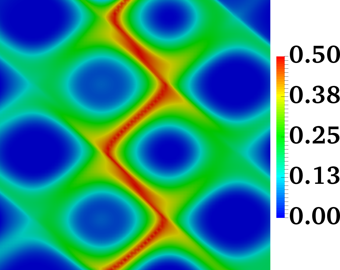
(a) $\kappa_{\mathrm{f}}L=2$ and $t=0.1$

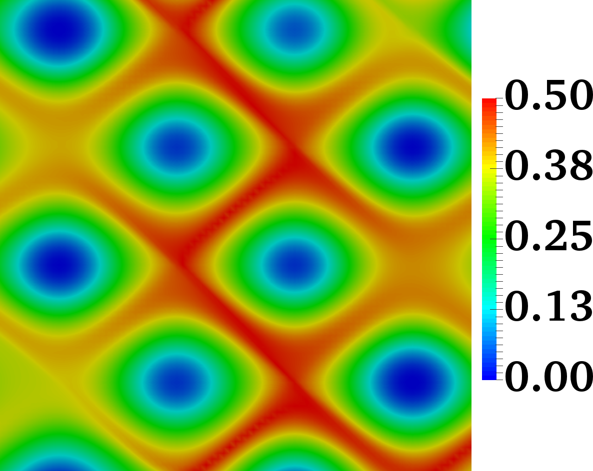
(b) $\kappa_{\mathrm{f}}L=2$ and $t=0.5$

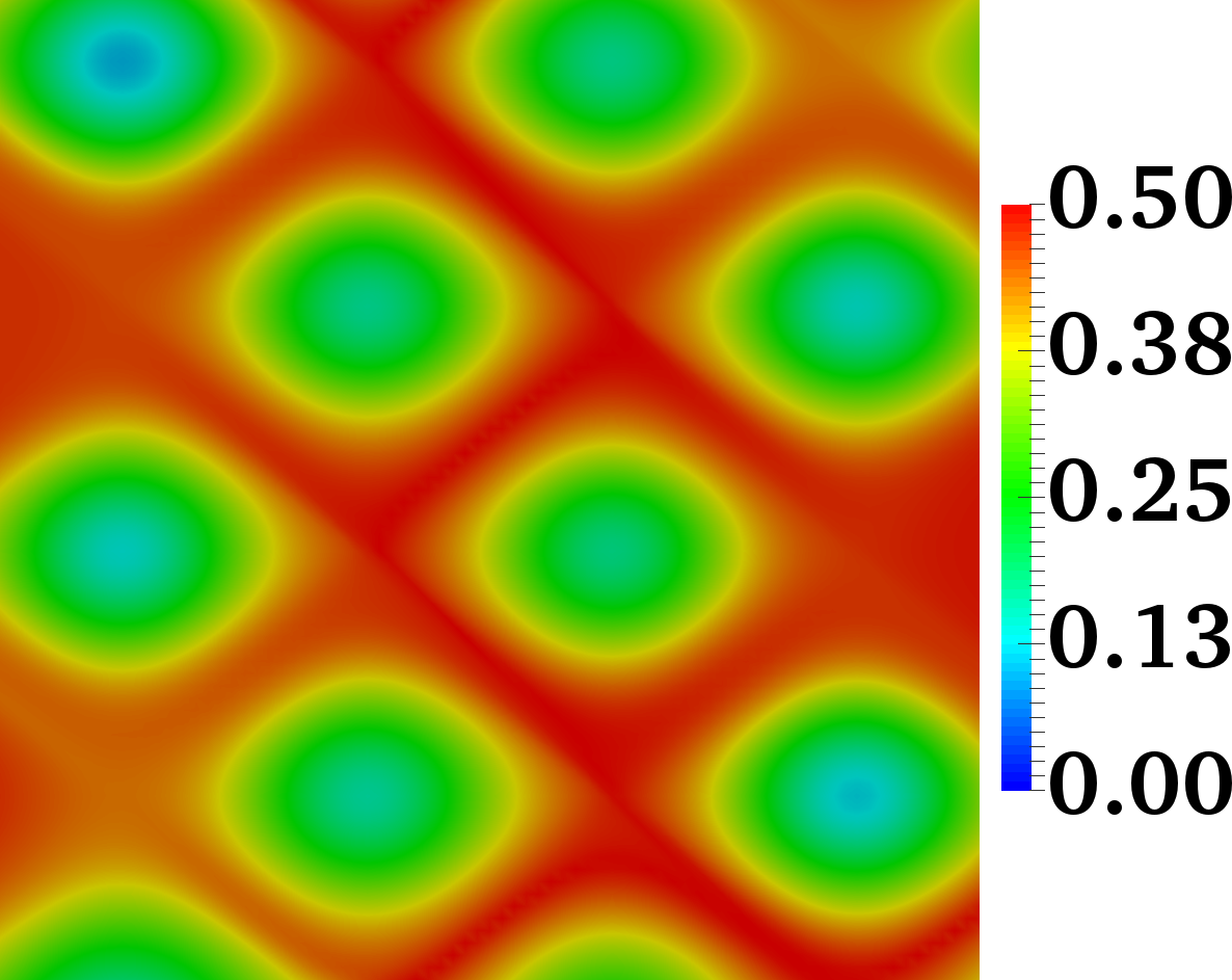
(c) $\kappa_{\mathrm{f}}L=2$ and $t=1.0$

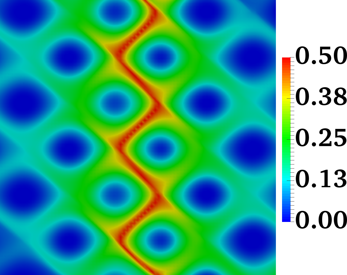
(d) $\kappa_{\mathrm{f}}L=3$ and $t=0.1$

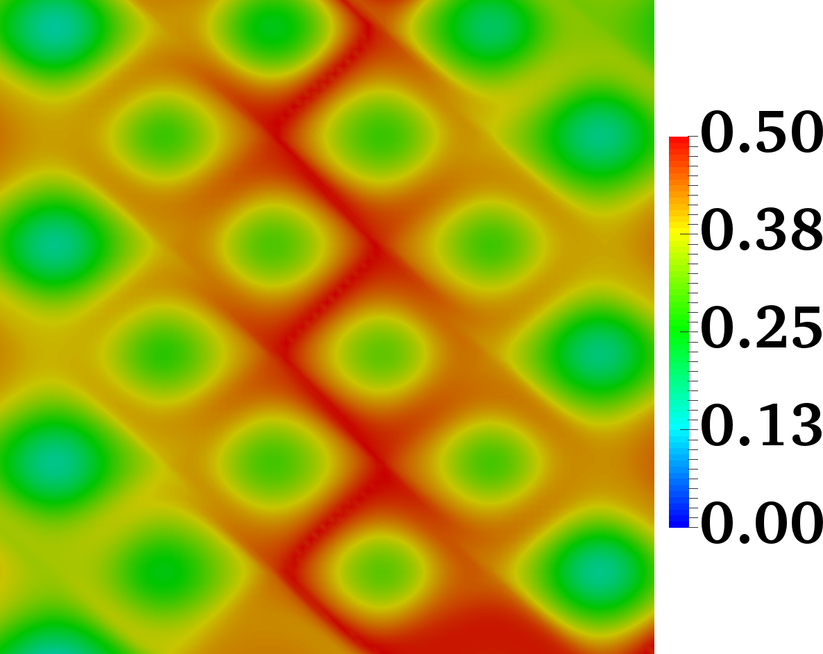
(e) $\kappa_{\mathrm{f}}L=3$ and $t=0.5$

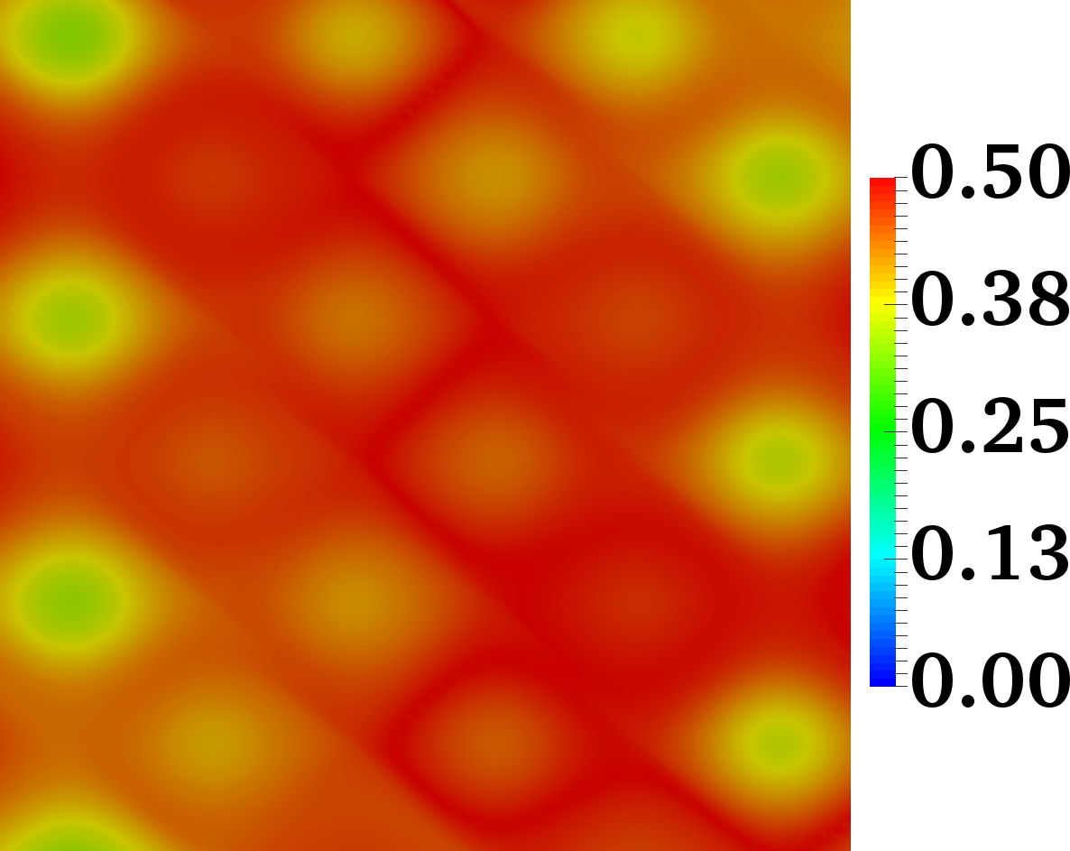
(f) $\kappa_{\mathrm{f}}L=3$ and $t=1.0$

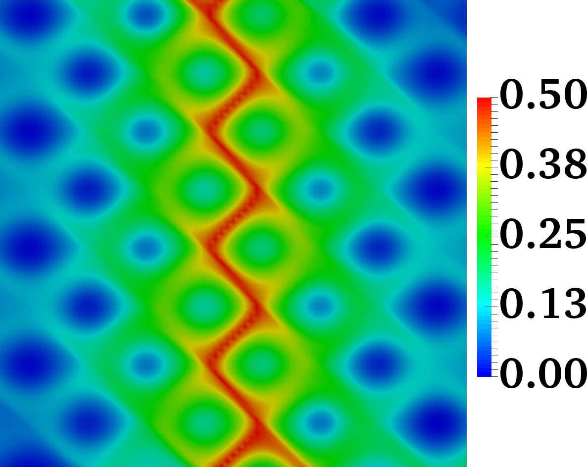
(g) $\kappa_{\mathrm{f}}L=4$ and $t=0.1$

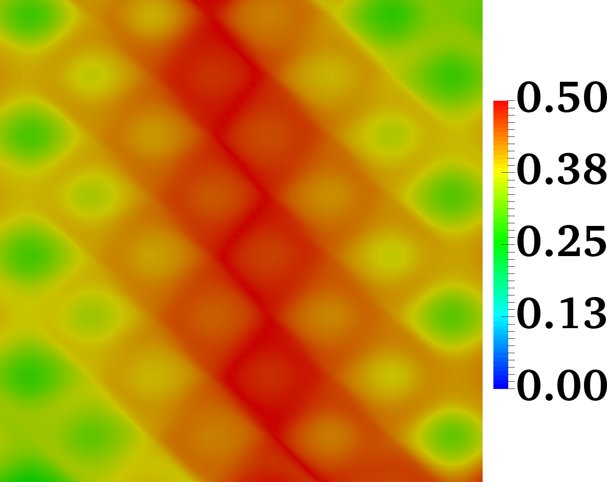
(h) $\kappa_{\mathrm{f}}L=4$ and $t=0.5$

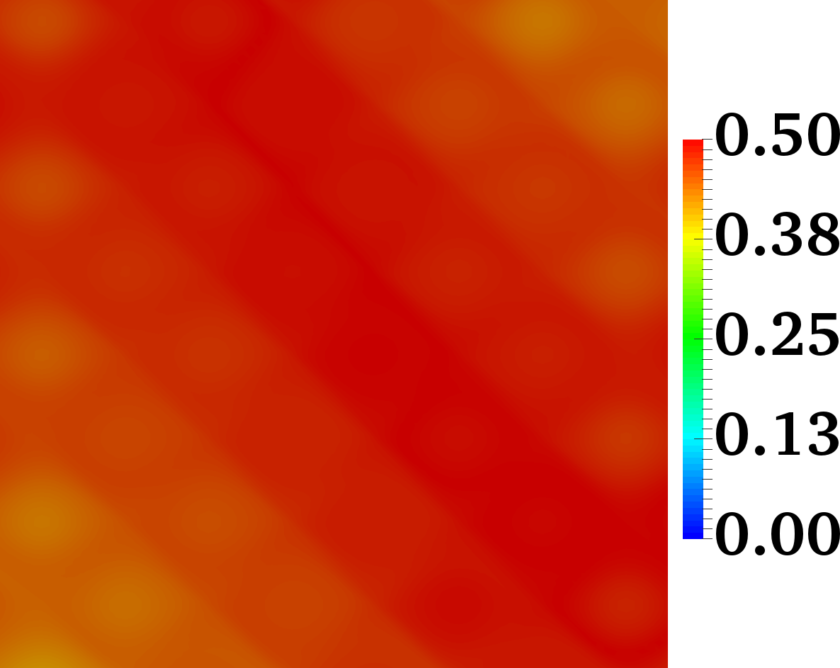
(i) $\kappa_{\mathrm{f}}L=4$ and $t=1.0$

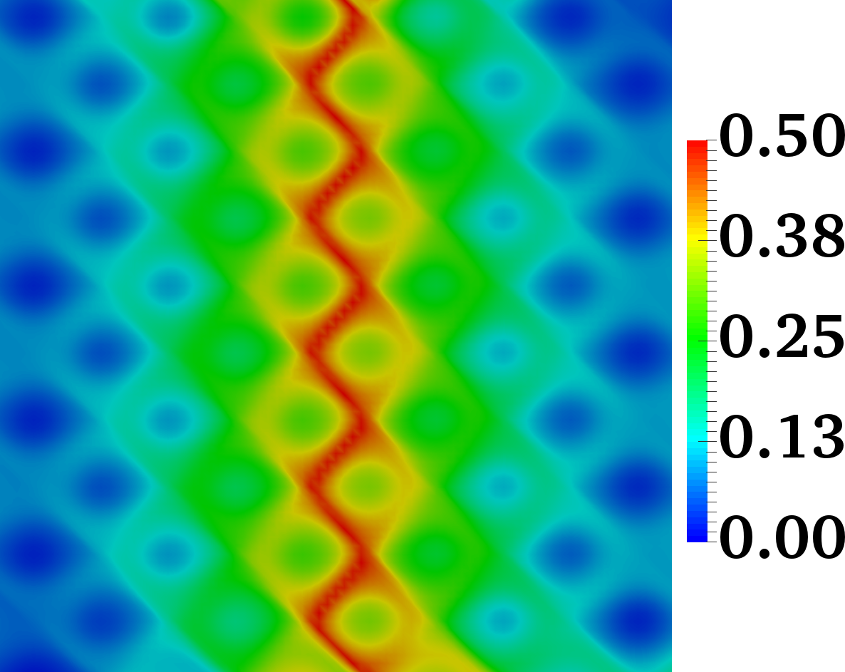
(j) $\kappa_{\mathrm{f}}L=5$ and $t=0.1$

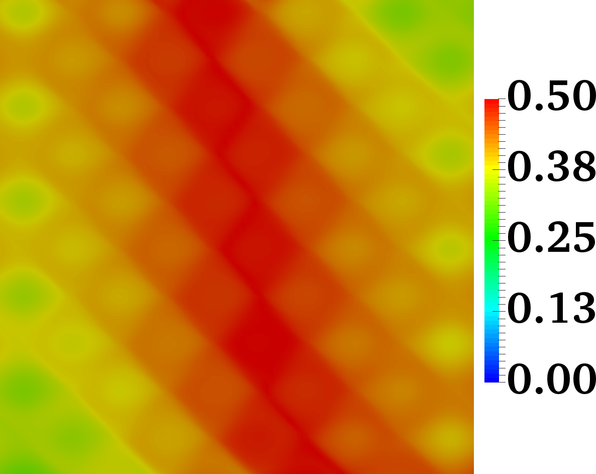
(k) $\kappa_{\mathrm{f}}L=5$ and $t=0.5$

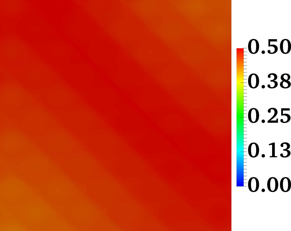
(l) $\kappa_{\mathrm{f}}L=5$ and $t=1.0$

Figure 2. Concentration contours of species $C$ under high anisotropy: Concentration of product $C$ at times $t=0.1,\,0.5,$ and $1.0$. Other input parameters were $\frac{\alpha_{\mathrm{L}}}{\alpha_{\mathrm{T}}}=10^{3}$ (high anisotropy), $v_{0}=1$, $T=0.1$, and $D_{\mathrm{m}}=10^{-3}$. Increased $\kappa_{\mathrm{f}}L$ increases $C$ production, especially at later times.

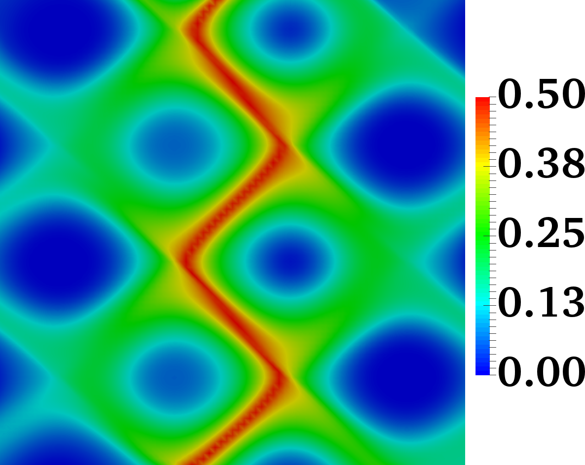
(a) $\kappa_{\mathrm{f}}L=2$ and $t=0.1$

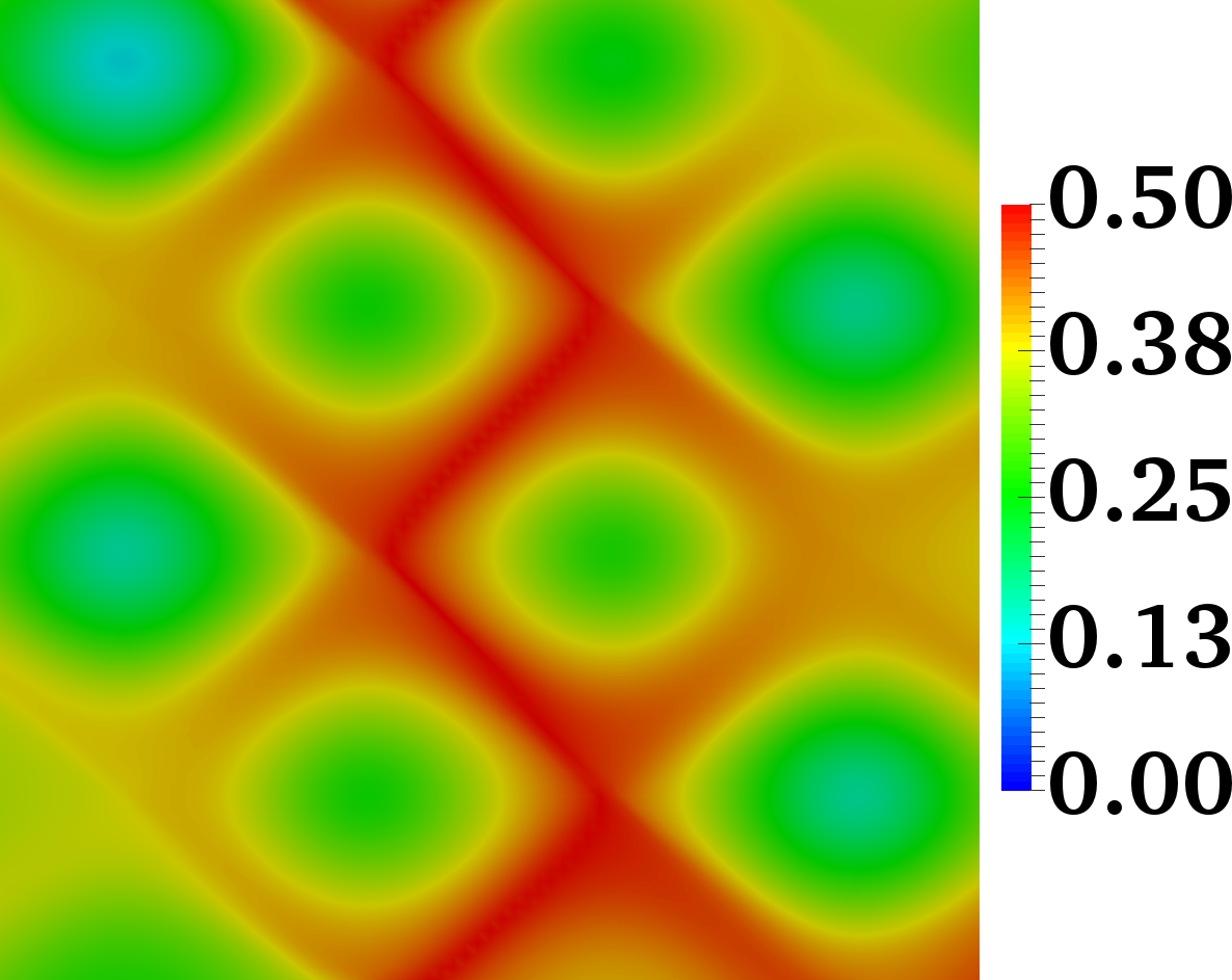
(b) $\kappa_{\mathrm{f}}L=2$ and $t=0.5$

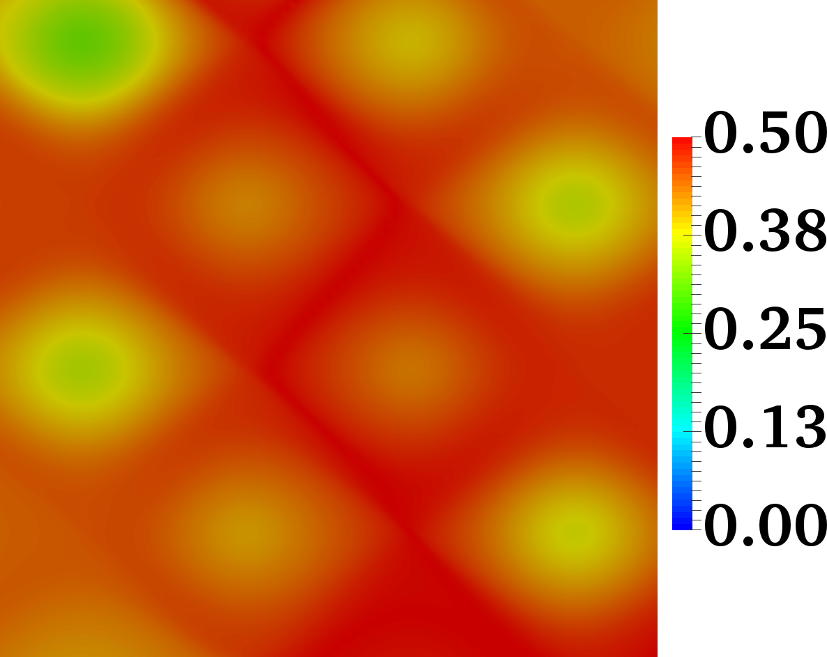
(c) $\kappa_{\mathrm{f}}L=2$ and $t=1.0$

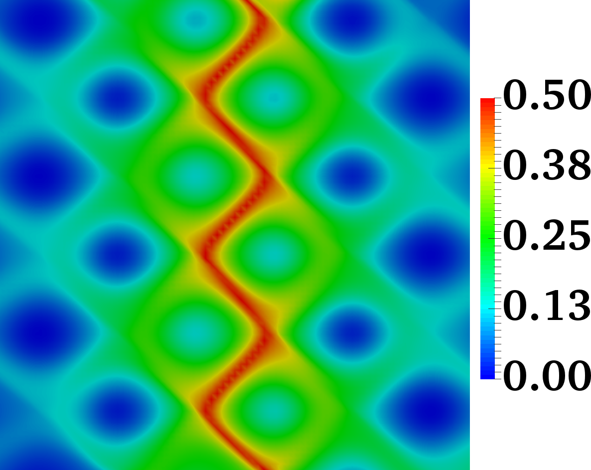
(d) $\kappa_{\mathrm{f}}L=3$ and $t=0.1$

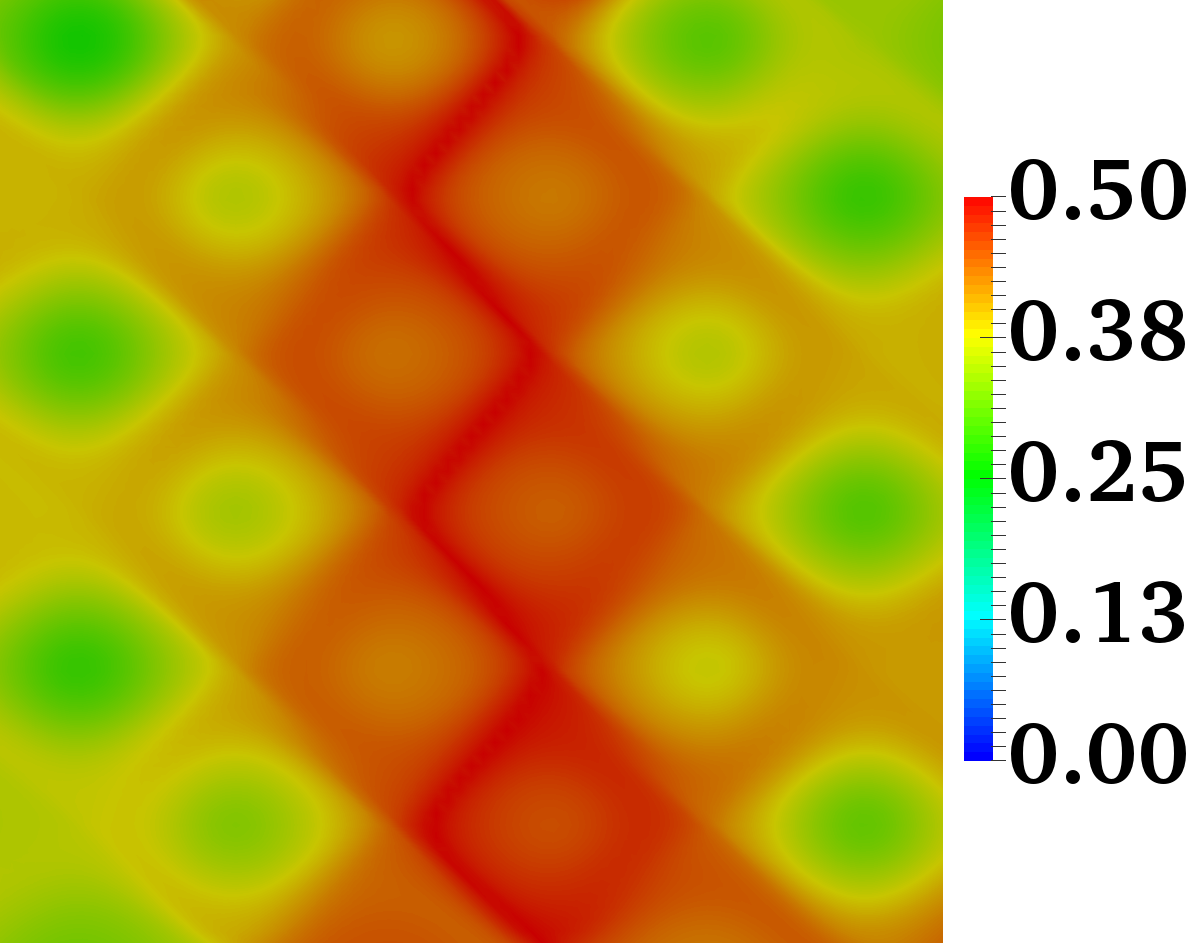
(e) $\kappa_{\mathrm{f}}L=3$ and $t=0.5$

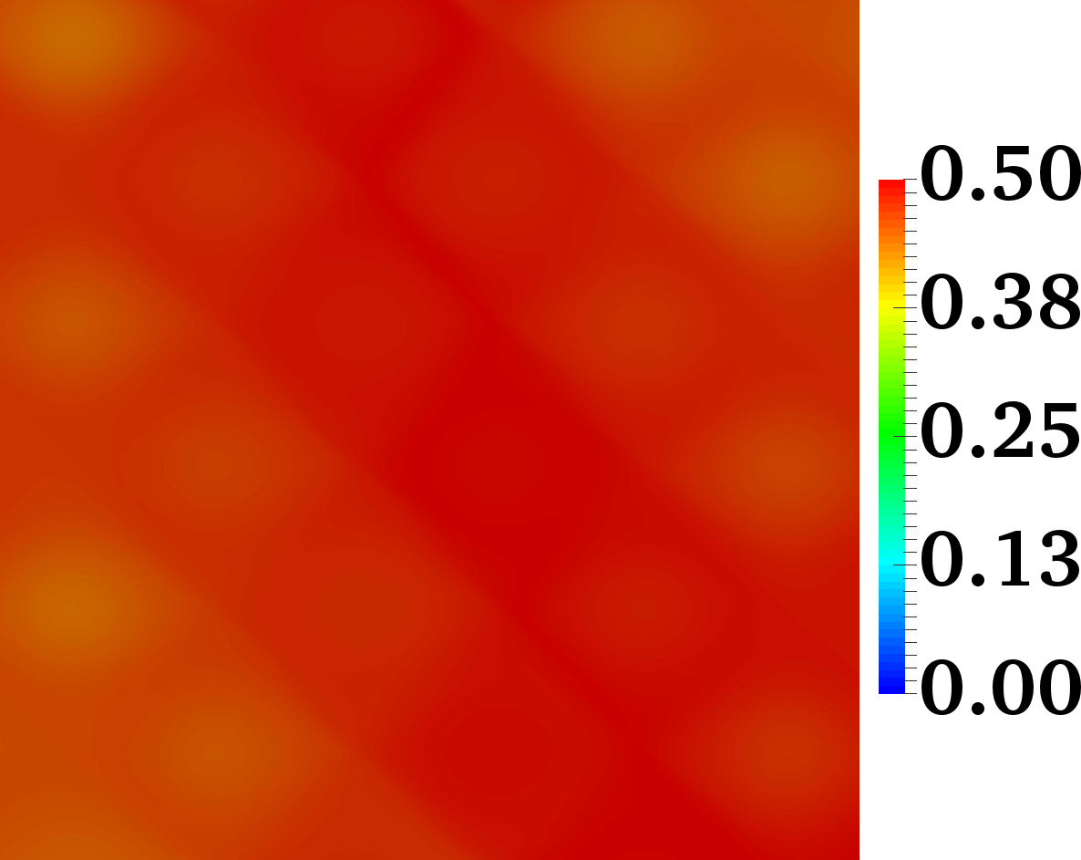
(f) $\kappa_{\mathrm{f}}L=3$ and $t=1.0$

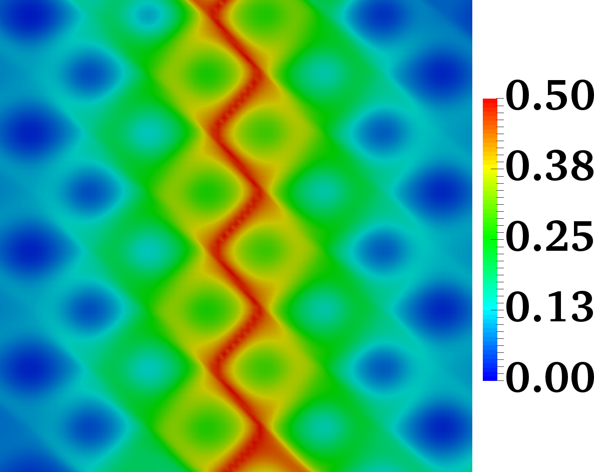
(g) $\kappa_{\mathrm{f}}L=4$ and $t=0.1$

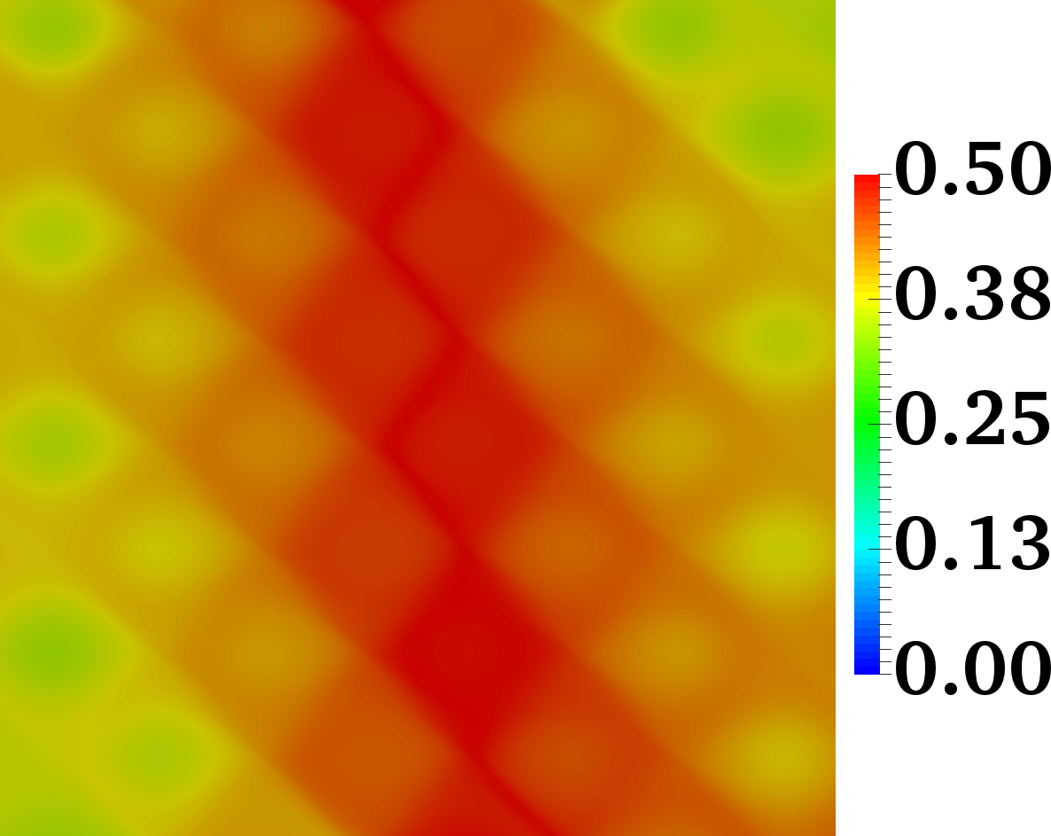
(h) $\kappa_{\mathrm{f}}L=4$ and $t=0.5$

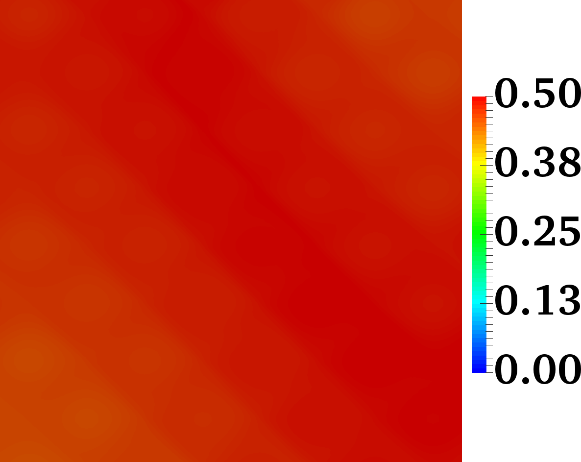
(i) $\kappa_{\mathrm{f}}L=4$ and $t=1.0$

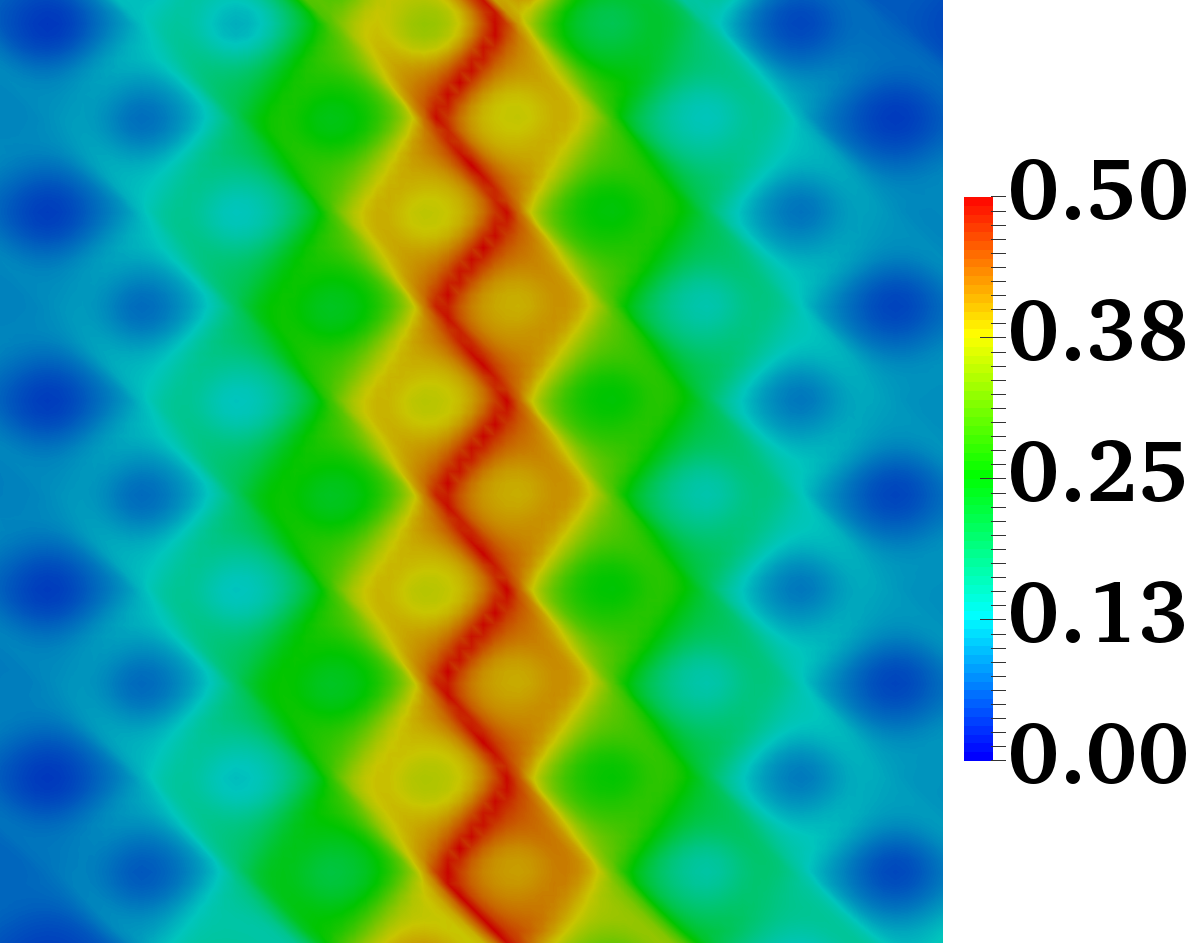
(j) $\kappa_{\mathrm{f}}L=5$ and $t=0.1$

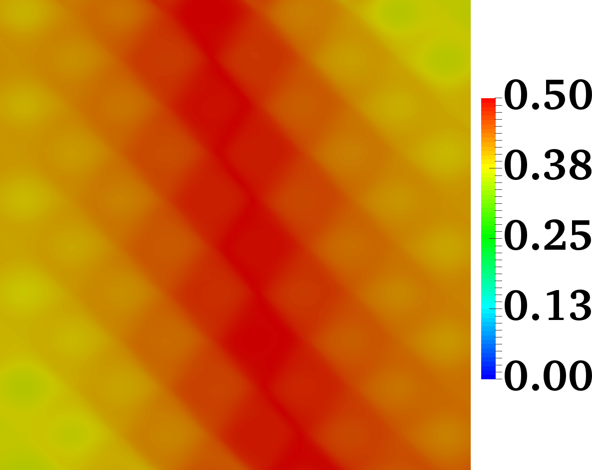
(k) $\kappa_{\mathrm{f}}L=5$ and $t=0.5$

(l) $\kappa_{\mathrm{f}}L=5$ and $t=1.0$

Figure 3. Concentration contours of species $C$ under medium anisotropy: Concentration of product $C$ at times $t=0.1,\,0.5,$ and $1.0$. Other input parameters were $\frac{\alpha_{\mathrm{L}}}{\alpha_{\mathrm{T}}}=100$ (medium anisotropy), $v_{0}=1$, $T=0.1$, and $D_{\mathrm{m}}=10^{-3}$. Lower anisotropy increased $C$ production than higher anisotropy in Fig. 2.

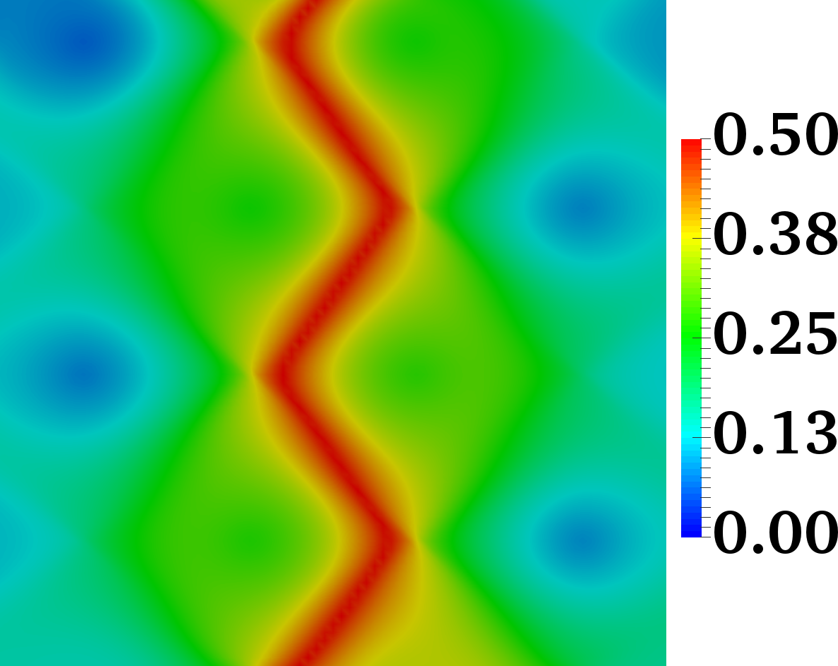
(a) $\kappa_{\mathrm{f}}L=2$ and $t=0.1$

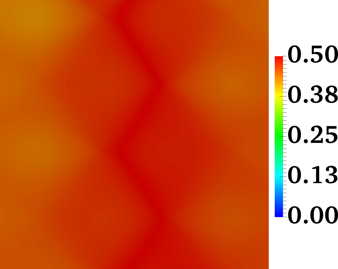
(b) $\kappa_{\mathrm{f}}L=2$ and $t=0.5$

(c) $\kappa_{\mathrm{f}}L=2$ and $t=1.0$

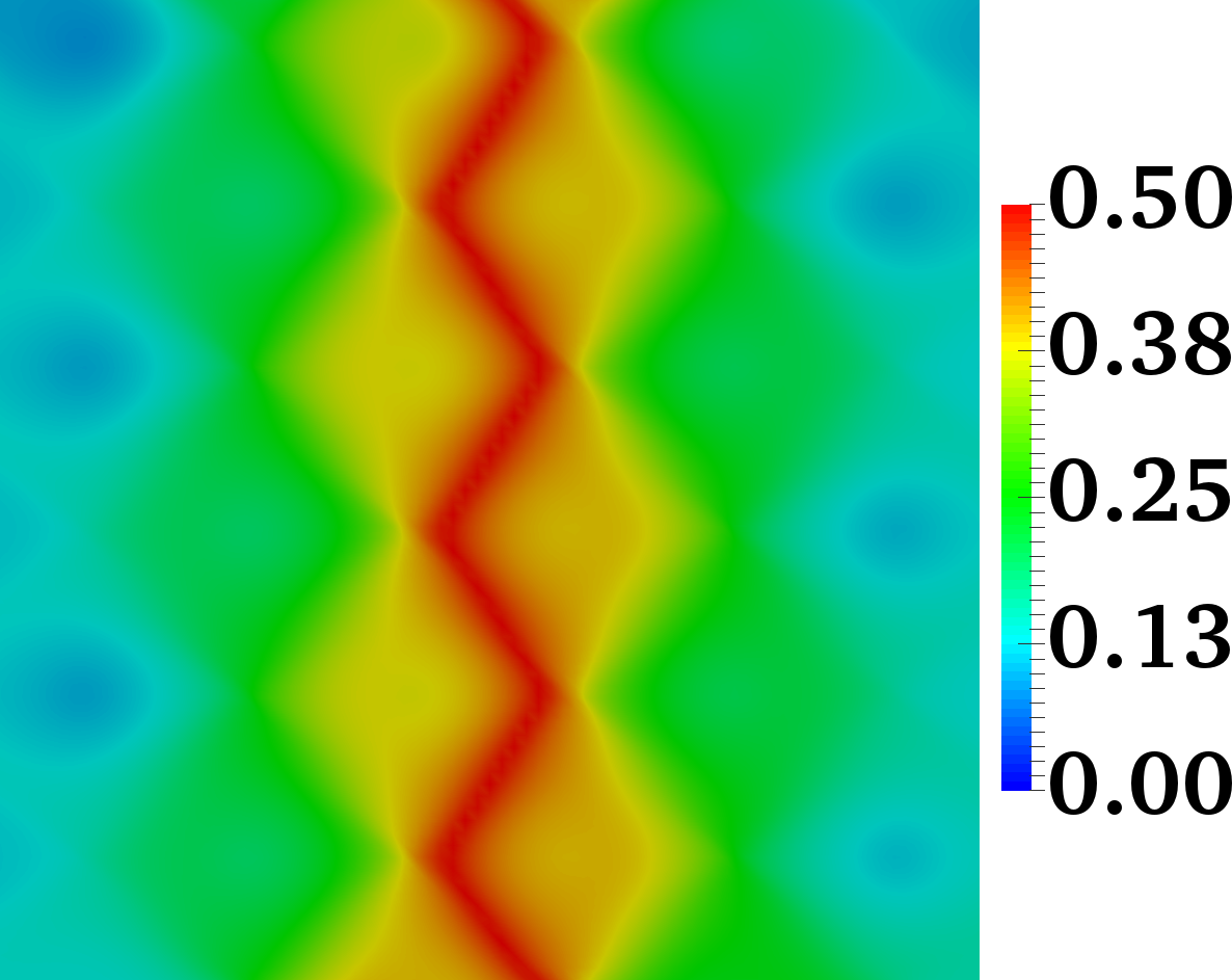
(d) $\kappa_{\mathrm{f}}L=3$ and $t=0.1$

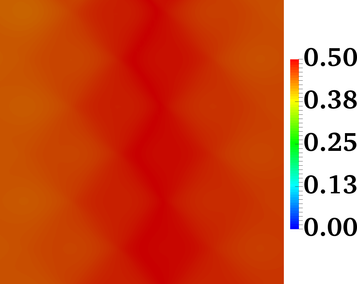
(e) $\kappa_{\mathrm{f}}L=3$ and $t=0.5$

(f) $\kappa_{\mathrm{f}}L=3$ and $t=1.0$

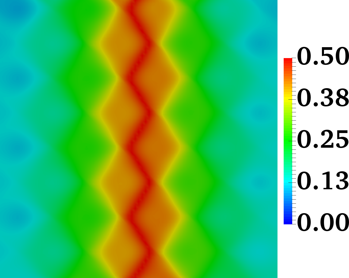
(g) $\kappa_{\mathrm{f}}L=4$ and $t=0.1$

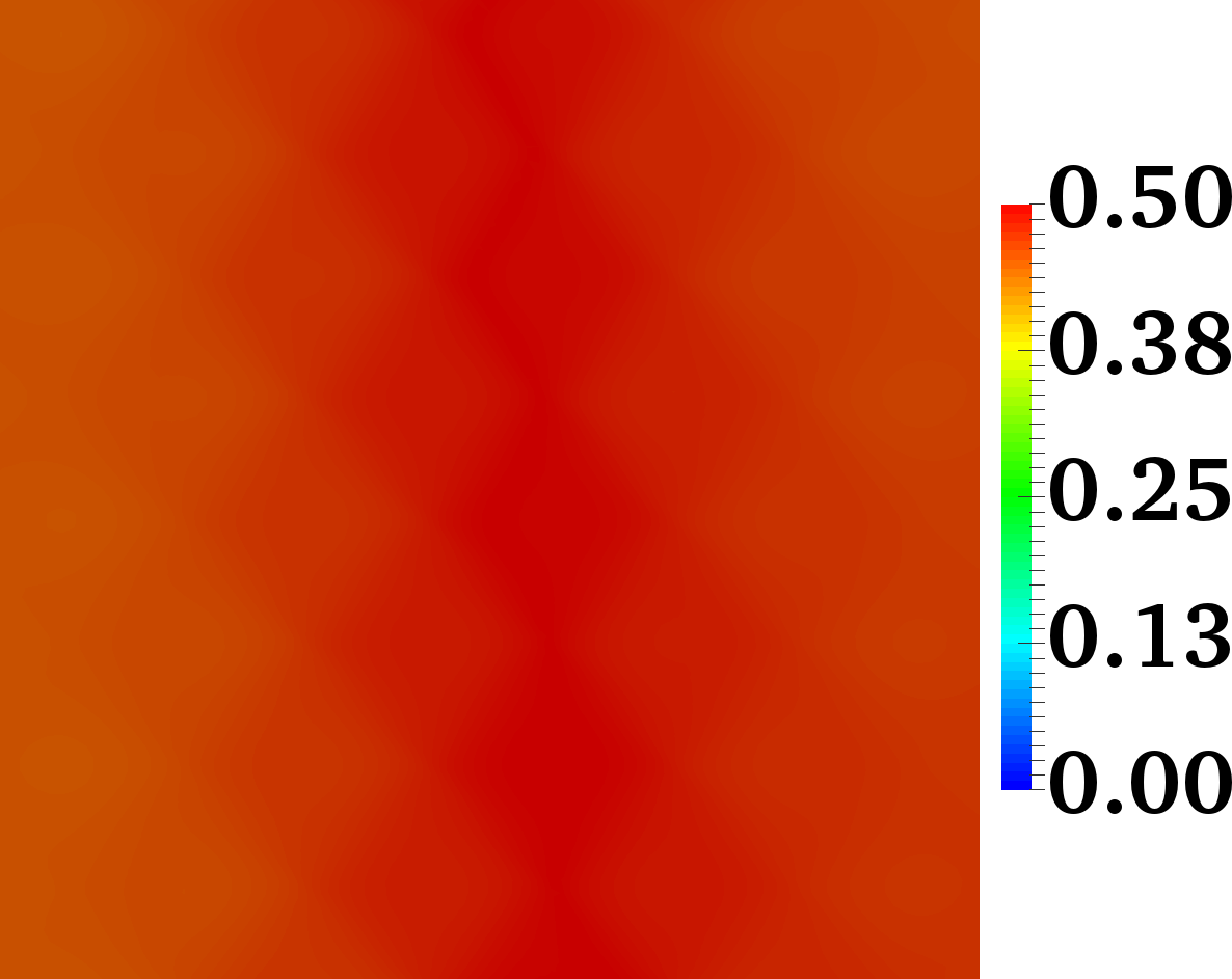
(h) $\kappa_{\mathrm{f}}L=4$ and $t=0.5$

(i) $\kappa_{\mathrm{f}}L=4$ and $t=1.0$

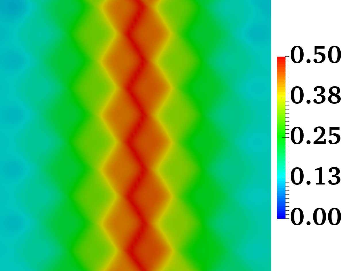
(j) $\kappa_{\mathrm{f}}L=5$ and $t=0.1$

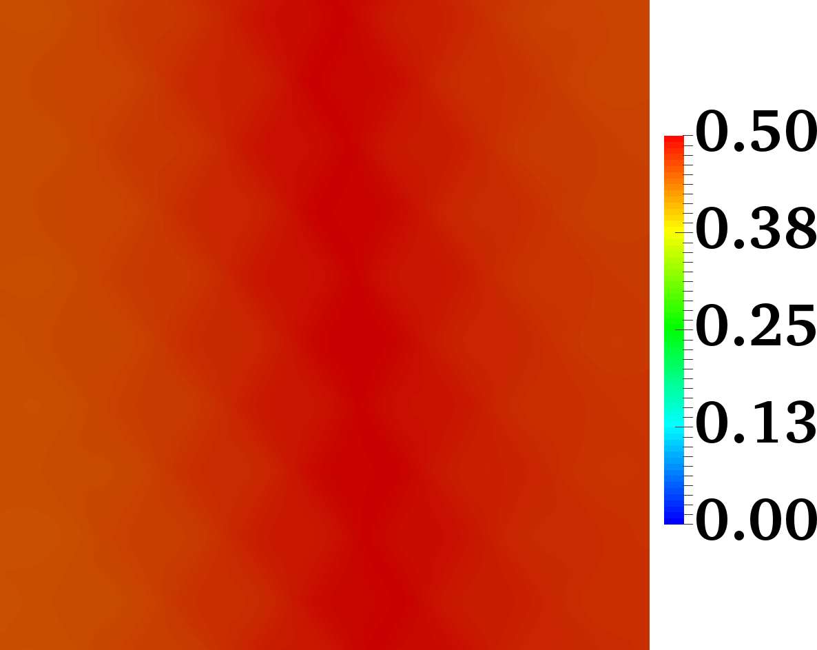
(k) $\kappa_{\mathrm{f}}L=5$ and $t=0.5$

(l) $\kappa_{\mathrm{f}}L=5$ and $t=1.0$

Figure 4. Concentration contours of species $C$ under low anisotropy: Concentration of product $C$ at times $t=0.1,\,0.5,$ and $1.0$. Other input parameters were $\frac{\alpha_{\mathrm{L}}}{\alpha_{\mathrm{T}}}=10$ (low anisotropy), $v_{0}=1$, $T=0.1$, and $D_{\mathrm{m}}=10^{-3}$. At low anisotropy, production of $C$ increased. During late times (e.g., $t=0.5$ and $1.0$), diffusion dominates $C$ production while $\kappa_{\mathrm{f}}L$ and $\frac{\alpha_{\mathrm{L}}}{\alpha_{\mathrm{T}}}$ minimally affect $C$ production.

After time $t=0$, reactants $A$ and $B$ are allowed to mix and form product $C$. The extent of mixing depended upon the reaction-diffusion inputs (features). Increased degree of mixing increases the yield of product $C$. Product $C$ yield at normalized simulation times $t=0$, 0.5, and 1.0 are shown in Figs. 2-4 revealing the significance of $k_{\mathrm{f}}L$ on product formation at different times. The importance of $\frac{\alpha_{\mathrm{L}}}{\alpha_{\mathrm{T}}}$ on product formation at various times was also evident. For $k_{\mathrm{f}}L=2$ and $\frac{\alpha_{\mathrm{L}}}{\alpha_{\mathrm{T}}}=10^{3}$ (see Fig. 2 (a-c)) at $t=0.1$, there is little reaction at the center of the vortices. However, regions with zero concentration decrease as $k_{\mathrm{f}}L$ increases. For example, at $k_{\mathrm{f}}L=3$ and $t=1.0$, more product is formed and negligible zero concentration of $C$ is present in the model domain. At $k_{\mathrm{f}}L=5$ and $t=1.0$, the system is nearly well-mixed even at high anisotropy. Because high $k_{\mathrm{f}}L$ creates a higher number of vortices that enhance reactant mixing, it increases product yield. Figure 3 shows the product $C$ yield under medium anisotropy. Reducing anisotropy ($\frac{\alpha_{\mathrm{L}}}{\alpha_{\mathrm{T}}}$) from 1,000 to 100 improve product yield even under low $\kappa_{\mathrm{f}}L$ (see Fig. 3(c)). Among $\frac{\alpha_{\mathrm{L}}}{\alpha_{\mathrm{T}}}$, $k_{\mathrm{f}}L$, and $D_{\mathrm{m}}$, $\frac{\alpha_{\mathrm{L}}}{\alpha_{\mathrm{T}}}$ controls the reaction at early times while $k_{\mathrm{f}}L$ and $D_{\mathrm{m}}$ controls reaction at late times. Higher values of $\frac{\alpha_{\mathrm{L}}}{\alpha_{\mathrm{T}}}$ decreases product yield but higher values of $k_{\mathrm{f}}L$ and $D_{\mathrm{m}}$ increases the product yield.

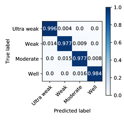
(a) Species $C$: RF

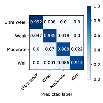
(b) Species $C$: MLP

Figure 5. Confusion matrices classifying the degree of mixing for the RF (left) and MLP (right) emulators.

ML emulators are also used to classify the mixing state of the system. Out of 20 ML emulators, only LogR, LDA, QDA, RF, and MLP are used for classification. Table 8 shows the training score, testing score, sample sizes, and training time for each linear ML emulator. Because the progress of reactive-mixing is nonlinear, linear ML emulators (e.g., LogR, LDA, QDA) fail to learn an accurate function for the state of mixing. Mixing state classification by linear classifiers on training and testing data have accuracies <80%. Nonlinear classifiers such as RF and MLP learn better functions are quite accurate, >95%. Results from RF and MLP are used to plot the confusion matrix of Figure 5 to show true and false predictions. Confusion matrix for RF and MLP are constructed using approximately 1% of data (23 simulations as training data) while the remaining 99% (2,292 simulations) data are used as testing data. In the confusion matrix, diagonal and off-diagonal elements show true and false predictions, respectively. The RF and MLP emulators false prediction scores are less than 2% and 10%, respectively. Similar trends are observed for species $A$ and $B$, hence the confusion matrices for them are not shown here.

Table 9 shows the training and testing scores for the six linear ML emulators. Although training times are short (always <20 minutes), training and testing $R^{2}$ scores never exceed 73%. Also, we apply three Bayesian ML emulators (e.g., BR, GP, NB) to predict QoIs that show similar performance as linear emulators. Among them, training and testing scores of BR and NB are <75%. GPs fail to converge for large datasets because of lack of sparsity and due to large training sample size ($\approx\mathcal{O}(10^{4})-\mathcal{O}(10^{6})$); however, GP trained on a smaller sample size scores >99%. This increased prediction capability of GP compared to other Bayesian ML emulators can be attributed to the RBF kernels. As species $A$ and $B$ decay or product $C$ increases in an exponential fashion, RBF kernels used by GP emulators are better suited to model such a reactive-mixing system. Hence, GP emulators trained on small (0.25% of data) data perform best and show promise to predict QoIs.

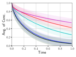
(a) Species $A$: $\mathfrak{c}_{A}$

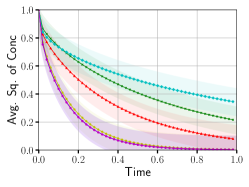
(b) Species $A$: $\mathbb{c}_{A}$

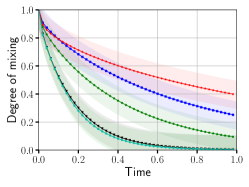
(c) Species $A$: $\sigma^{2}_{A}$

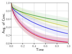
(d) Species $B$: $\mathfrak{c}_{B}$

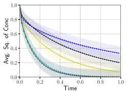
(e) Species $B$: $\mathbb{c}_{B}$

(f) Species $B$: $\sigma^{2}_{B}$

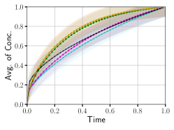
(g) Species $C$: $\mathfrak{c}_{C}$

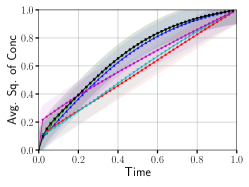
(h) Species $C$: $\mathbb{c}_{C}$

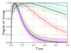
(i) Species $C$: $\sigma^{2}_{C}$

Figure 6. Predictions of QoIs by Random Forest emulators for the six unseen realizations: This figure shows the true (markers) and RF emulator predictions (solid curves) of average concentrations, squared of average concentrations, and degree of mixing (a)–(c) of species $A$; (d)–(f) of species $B$, and (g)–(i) of species $C$.

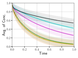
(a) Species $A$: $\mathfrak{c}_{A}$

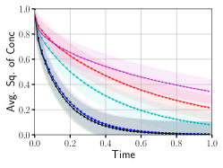
(b) Species $A$: $\mathbb{c}_{A}$

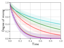
(c) Species $A$: $\sigma^{2}_{A}$

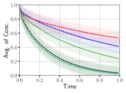
(d) Species $B$: $\mathfrak{c}_{B}$

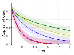
(e) Species $B$: $\mathbb{c}_{B}$

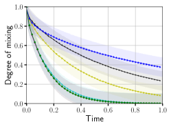
(f) Species $B$: $\sigma^{2}_{B}$

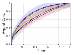
(g) Species $C$: $\mathfrak{c}_{C}$

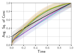
(h) Species $C$: $\mathbb{c}_{C}$

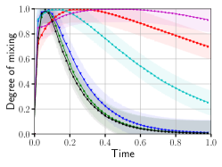
(i) Species $C$: $\sigma^{2}_{C}$

Figure 7. Predictions of QoIs by GBM emulators for the six unseen realizations: This figure shows the true (markers) and GBM emulator predictions (solid curves) of average concentrations, squared of average concentrations, and degree of mixing (a)–(c) of species $A$; (d)–(f) of species $B$, and (g)–(i) of species $C$.

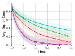
(b) Species-$A$: $\mathbb{c}_{A}$

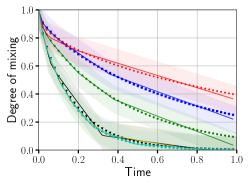
(c) Species-$A$: $\sigma^{2}_{A}$

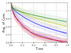
(d) Species-$B$: $\mathfrak{c}_{B}$

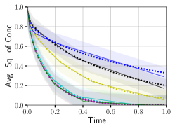
(e) Species-$B$: $\mathbb{c}_{B}$

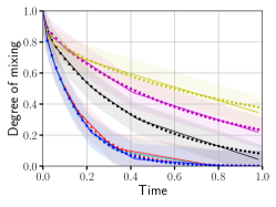
(f) Species-$B$: $\sigma^{2}_{B}$

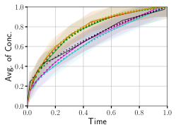
(g) Species-$C$: $\mathfrak{c}_{C}$

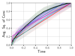
(h) Species-$C$: $\mathbb{c}_{C}$

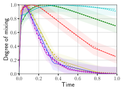
(i) Species-$C$: $\sigma^{2}_{C}$

Figure 8. Predictions of QoIs by ANN emulators for the six unseen realizations: This figure shows the true (markers) and ANN emulator predictions (solid curves) of average concentrations, squared of average concentrations, and degree of mixing (a)–(c) of species $A$; (d)–(f) of species $B$, and (g)–(i) of species $C$.

Table 10 compares the training and testing scores for ensemble and MLP emulators. The ${R}^{2}$ scores for training and testing datasets are greater than 90% (e.g., Bagging, DT, RF, MLP). For six unseen (blind) realizations, Bagging, DT, RF, AdaBoost, DT-based AdaB, and GBM show astounding match between true QoIs and their corresponding predictions by RF and GBM. Here, only figures for RF and GBM emulators (see, Figures 6–7) are shown here because the remaining ensemble emulators show the similar trend. These results indicate that tree-based methods outperform linear ML methods in capturing the QoIs of the reactive-mixing system. Also, Figure 8 shows the QoIs predictions by the MLP emulator for the six blind realizations. The test ${R}^{2}$ score (>99%) on different data sizes and generalized cross-validation during emulator development indicate that overfitting is not a problem. As the size of the training dataset increases, the ensemble and MLP emulator development time increase.

Finally, the computational costs to run the high-fidelity model and the ML emulators are investigated. Tables 8–10 compare the computational cost of development of various ML emulators. These tables provide details on training time for various training dataset sizes on a 32-core processor (Intel(R) Xeon(R) CPU E5-2695 v4 2.10GHz). A single, high-fidelity numerical simulation requires approximately 1,500 s on a single core. Testing an ML emulator (e.g., RF, MLP) takes 0.01–0.1 s about 1/100,000^th of the time of the high-fidelity numerical simulation.

Table 8. Performance metrics of ML emulators on training and test datasets for classifying the mixing state (i.e., degree of mixing) of the reaction-diffusion system.

Emulator	Training	Testing	Training	Testing	Training
	size (%)	size (%)	score (%)	score (%)	time (s)
LogR	0.9	99	75	75	31
	63	30	75	75	138
	81	10	75	75	174
LDA	0.9	99	72	72	28
	63	30	72	72	93
	81	10	72	72	102
QDA	0.9	99	77	77	66
	63	30	77	77	128
	81	10	77	77	133
RF	0.9	99	100	98	6,527
	63	30	100	99	22,161
	81	10	100	99	24,015
MLP	0.9	99	97	96	3,384
	63	30	99	99	50,397
	81	10	99	99	66,381

Table 9. Performance metrics of linear and Bayesian ML emulators (regressors). Note, GP and KR failed to converge even on 1% of training data because of a memory leak due to storage of a dense matrix.

Emulator	Training	Testing	Training	Testing	Training
	size (%)	size (%)	score (%)	score (%)	time (s)
LSQR	0.9	99	69	69	12
	63	30	69	69	52
	81	10	69	69	57
RR	0.9	99	69	69	10
	63	30	69	69	42
	81	10	69	69	50
LR	0.9	99	69	69	95
	63	30	69	69	330
	81	10	69	69	368
ER	0.9	99	69	69	121
	63	30	69	69	1,077
	81	10	69	69	1,227
HR	0.9	99	69	69	14
	63	30	69	69	185
	81	10	69	69	195
Polynomial	0.9	99	89	89	79
	63	30	89	99	143
	81	10	89	89	164
BR	0.9	99	69	69	12
	63	30	69	69	62
	81	10	69	69	69
NB	0.9	99	73	73	69
	63	30	73	73	73
	81	10	73	73	91

Table 10. Performance metrics of ensemble and MLP emulators.

Emulator	Training	Testing	Training	Testing	Training
	size (%)	size (%)	score (%)	score (%)	time (s)
DT	0.9	99	100	99	42
	63	30	99	99	100
	81	10	99	99	110
Bagging	0.9	99	98	95	42
	63	30	98	95	110
	81	10	98	95	100
RF	0.9	99	100	99	1,435
	63	30	100	99	5,468
	81	10	100	99	6,044
AdaB	0.9	99	90	90	72
	63	30	89	89	1,378
	81	10	89	89	1,585
DT-based AdaB	0.9	99	99	99	103
	63	30	99	99	1,648
	81	10	99	99	1,778
GBM	0.9	99	98	98	133
	63	30	98	98	1,533
	81	10	98	98	2,048
MLP	0.9	99	99	99	688
	63	30	99	99	4,678
	81	10	99	99	9,691

5   Discussion

A suite of linear, Bayesian, and nonlinear ML emulators are trained to classify and replicate QoIs from high-fidelity anisotropic bi-linear diffusion numerical simulations. For this highly nonlinear system, linear and Bayesian ML emulators never exceed 70% classification accuracy while LogR and QDA achieve only 75% and 77% classification accuracies, respectively. On the other hand, nonlinear emulators perform well (95% classification accuracies for RF and MLP). For the regression problem (predicting the three QoIs for each chemical species), as expected, linear regressors predict QoIs at only $R^{2}=69$%, but decision-tree-based ensembles and the MLP neural network perform remarkably well. DTs (with and without AdaBoost), RFs, and the MLP all had $R^{2}=99$% with GBM (98%), bagging (95%), and AdaBoost (85%) performs somewhat worse.

These results indicate that ensemble emulators outperform other ML emulators in predicting the progress of reactive mixing on unseen data. However, not all of them perform equally. For example, RF outperforms other averaging ensembles (e.g., Bagging, DT) while DT-based AdaB outperforms other boosting methods (e.g., AdaB, GBM). Each bagging/averaging ensemble methods introduce randomness and voting-based evaluation metrics in unique ways; therefore, their performance is not the same. For example, DTs often use the first feature to split; resultantly, the order of variables in the training data is critical for DT-based model construction. Also, in DTs, trees are pruned and not fully grown. Contrarily, RF can have unpruned and fully grown trees and are not sensitive to the feature order as in DTs. Also, each tree in an RF learns using random sampling, and at each node, a random set of features are considered for splitting. This random sampling and splitting introduces diversity among trees in a forest. After randomly selecting features, RF builds a number of regression trees and averages (aka bagging) them. With enough trees, combinations of randomly selected features and averaging (aka voting), RF emulators reduce the variance of predictions and deter the overfitting. Resultantly, their performances are best among all averaging ensemble emulators.

Among boosting methods, DT-based AdaB outperforms AdaB and GBM because it combines DT and boosting estimators to predict QoIs. In this study, the DT-based AdaB uses 100 trees as a base estimator to build DT-based AdaB emulator. Two base estimators enhance the confidence on QoI predictions; resultantly, the DT-based AdaB emulator scores better than other two boosting approaches. Based on the ML analyses presented in Sec. 4, linear and Bayesian ML emulators (e.g., NB, BR, GP) are a poor choice to classify and predict reactive-mixing QoIs. Overall, RF, DT-based AdaB, GBM, and MLP emulators accurately predicted unseen realizations with average accuracies >90%. From the computational-cost perspective, generalized linear and Bayesian ML emulators are faster to train than ensemble and MLP emulators. Among ensemble and boosting methods, RF and GBM emulators take longest to train. Also, MLP emulators are more expensive to develop than other ML emulators. However, ensemble and MLP emulators take 1/100,000^th of the time required for a high-fidelity simulation to predict equivalent QoIs.

6   Conclusions

Our primary purpose was to accurately understand reactive-mixing state and expedite predictions of species concentration (QoIs) due to reactive mixing. A suite of linear, Bayesian, ensemble, and MLP ML emulators were compared to classify the state of reactive mixing and to predict species concentrations. All ML emulators were developed based on high-fidelity numerical simulation datasets. A total of 2,315 simulations were carried out to generate data to train and test the emulators. Data were generated by solving the anisotropic reaction-diffusion equations using the non-negative finite element method. Because of the highly nonlinear reactive-mixing system, linear and Bayesian (except GP) ML emulators performed poorly in classifying and predicting the state of reactive mixing (e.g., $R^{2}$ $\approx$ 70%). Among Bayesian ML emulators, GP showed promise for accurate prediction of QoIs for small datasets. On the other hand, ensemble and MLP emulators accurately classified the state of reactive-mixing and predicted associated QoIs. For example, RF and MLP emulators classified the state of reactive-mixing with an accuracy of >90%. Moreover, they predicted the progress of reactive-mixing with an accuracy of >95% on training, testing, and unseen data. Among bagging ensemble methods, RF emulators provided comparatively better predictions than bagging and DT emulators. Similarly, among boosting ensemble methods, DT-based AdaBoost emulators provided better predictions than AdaBoost and GBM emulators. Computationally, for QoI predictions, ML emulators were approximately $10^{5}$ faster than a high-fidelity numerical simulation. Finally, ensemble ML and MLP emulators proved good classifiers and predictors for interrogating the progress of reactive mixing. Looking to the future, ensemble ML and MLP emulators will be validated on both reservoir-scale field and simulation data.

Conflict of Interest

The authors declare that they do not have conflict of interest.

Computer Code Availability

Codes for machine learning implementation are available in the public Github repository https://github.com/bulbulahmmed/ML-to-reactive-mixing-data. Additional information regarding the simulation datasets can be obtained from Bulbul Ahmmed (Email: bulbul_ahmmed@baylor.edu) and Maruti Kumar Mudunuru (Email: maruti@lanl.gov).

(a) Species-$A$: $\mathfrak{c}_{A}$

Appendix A Appendices

A.1   Nomenclature

A.1.1   Variables

A = Diagonal matrix
$a_{n}^{l}$ = Activation function of neuron $n$ at layer $l$
$b$ = Bias
$c_{i}$ [mol m^-3] = The molar concentration of chemical species $i$
$c^{0}_{i}(\mathbf{x})$ = The initial concentration of chemical species $i$
$c^{\mathrm{p}}_{i}(\mathbf{x},t)$ [mol m^-3] = Prescribed molar concentration
$\mathbf{D}(\mathbf{x},t)$ [s${}^{2}\,$m^-1] = The anisotropic dispersion tensor
$D_{\mathrm{m}}$ [m${}^{3}\,$s^-2] = The molecular diffusivity
$\mathrm{det}$ = Determinant
$\mathbb{E}$ = Expectation
$F$ = Activation function
$f$ = Function
$f_{m}$ = $m^{\mathrm{th}}$ classifier
$G$ = Impurity
$H$ = Gini impurity function
$H_{e}$ = Truncation value for Huber loss
$h_{m}$ = Base learner/tree
$h^{\mathrm{p}}_{i}(\mathbf{x},t)$ [m s^-1] = Flux
$i$ = Index
$\mathbf{I}$ = The identity tensor
$\mathrm{inf}$ = The greatest upper bound
$J=\mathrm{sup}\left|\hat{y_{i}}-y_{i}\right|$
$j$ = Feature index
$k$ = Class variable index
$k_{AB}$ [m^-1] = The bi-linear reaction rate coefficient
$L$ = Loss function
$L_{1}$ = $L_{1}$ norm
$L_{2}$ = $L_{2}$ norm
$l$ = Layer index
$\mathrm{l}$ = The length of the ‘wiggles’ in sine function
$M$ = Number of training data
$m$ = Tree node index
$N$ = Gaussian or normal distribution
$n$ = Node number
$n_{A}$ = Stoichiometric coefficient for species $A$
$n_{B}$ = Stoichiometric coefficient for species $B$
$n_{C}$ = Stoichiometric coefficient for species $C$
$o$ = Random coefficient
$p$ [%] = Probability
$\mathrm{p}$ = The distance between repetitions of the sine function
$p_{mk}$ [%] = Probability at $mk^{\mathrm{th}}$ leaf
$Q$ = Data at tree node $m$
$q$ = Batch or subsample
$r$ = Random coefficient
$s$ = Split
$\mathrm{sup}$ = The least upper bound
$t_{m}$ = Threshold at which trees split
$u$ = Random coefficient
$\mathbf{v}$ [m s^-1] = The velocity vector field
$v_{0}$ = The perturbation parameter
$w$ = Coefficient
$\mathbb{w}$ = Coefficient vector
$w_{0}$ = Intercept
$\mathbb{X}$ = Feature matrix
$\mathbb{x}$ = Feature vector
$y$ = Label
$\mathbb{y}$ = Label vector
$\hat{y}$ = Approximation to $y$
$z$ = The dummy variable

A.1.2   Greek Symbols

$\alpha$ = Penalty/regularization parameter
$\alpha_{1}$ = Regularization parameter for $w$
$\alpha_{2}$ = Regularization parameter for $w$
$\alpha_{\mathrm{L}}$ [m${}^{2}\,$s^-1] = The longitudinal diffusivity
$\alpha_{\mathrm{T}}$ [m${}^{2}\,$s^-1] = The transverse diffusivity
$\beta$ = Regularization parameter
$\Gamma^{\mathrm{D}}_{i}$ = Dirichlet boundary condition
$\Gamma^{\mathrm{N}}_{i}$ = Neumann boundary condition
$\theta_{m}$ = Confidence in the prediction for $m^{\mathrm{th}}$ data
$\kappa_{\mathrm{f}}L$ and $T$ [–] = The characteristic spatial and temporal scales of the flow field
$\gamma$ = Learning rate
$\epsilon$ = Truncation value under which no penalty is associated with the training loss
$\eta$ = Noise
$\theta$ = Confidence function for prediction
$\mathscr{K}$ = Node number
$\mathcal{K}$ = Kernel
$\lambda$ = Spread of kernel
$\mu$ = Mean
$\nu$ = Integer
$\mathrm{\pi}$ = cos^–1(–1)
$\Sigma$ = The covariance matrix
$\boldsymbol{\Psi}$ = Vector of $\mathcal{N}\times 1$ size
$\mathrm{\omega}$ = Regularization parameter
$\mathbb{I}$ = Identity matrix
$\mathfrak{T}$ = Number of regression tree
$\mathbf{\Phi}$ = Design matrix of $\mathcal{N}\times(\mathcal{N}+1)$ size
$\omega$ = Regularization parameter

A.1.3   Mathematical Symbol

$\otimes$ = The tensor product
$\mathbb{1}$ = Indicator function (either 1 or 0)

A.2   Brief Mathematical Description of ML Emulators

A.2.1   Linear Emulators

Generalized Linear Emulators

Suppose there are $n$ features $x_{1}$ through $x_{n}$ that correspond to a label $y$. LSQR calculates the closest $\hat{y}$ by finding the best linear combination of features as:

$$\hat{y}\left(\mathbb{w},\mathbb{x}\right)=w_{0}+w_{1}x_{1}+\cdots+w_{n}x_{n}=\mathbb{x}\cdot\mathbb{w}.$$ (12)

Linear regressors minimize a loss (or cost) function. The cost/loss function in this case is the residual sum of squares between a set of training feature vectors $\mathbb{x}_{1},\mathbb{x}_{2},\cdots,\mathbb{x}_{m}$ and predicted targets $y_{1},y_{2},\cdots,y_{m}$ of the form:

$$L_{\mathrm{lin}}=\underset{\mathbb{w}}{\mathrm{min}}||\mathbb{X}\mathbb{w}-\mathbb{y}||_{2}^{2}+\alpha_{1}||\mathbb{w}||_{1}+\alpha_{2}||\mathbb{w}||_{2}^{2}+\Sigma\sum_{i=1}^{m}\left[1+H_{\epsilon}\left(\frac{\mathbb{x}_{i}\cdot\mathbb{w}-y_{i}}{\Sigma}\right)\right].$$ (13)

For LSQR, $\alpha_{1}=\alpha_{2}=\Sigma=0$, for RR, $\alpha_{1}=\Sigma=0$, for LR, $\alpha_{2}=\Sigma=0$, for ER, $\Sigma=0$, and for HR, $\alpha_{2}=0$.

$$H_{\epsilon}\left(e\right)=\begin{cases}e^{2}&\mathrm{if}\,e<\,\epsilon\\ 2\epsilon|e|-\epsilon^{2}&\mathrm{otherwise}\\ \end{cases}.$$ (14)

The LSQR method minimizes $L_{\mathrm{lin}}$ without regularization. RR uses the $L_{2}$ norm, which does not use sparsity constraints. However, it includes a penalty $\alpha_{2}$ to weights, which is known as the ridge coefficient. This prevents weights from getting too large as well as overfitting. LR is another linear regressor that penalizes the $L_{1}$ norm. This penalty $\alpha_{1}$ on the absolute value of weights results in sparse models tending toward small weights. The $\alpha_{1}$ controls the strength of the regularization penalty, and more parameters are eliminated with increasing $\alpha_{1}$. With increasing $\alpha_{1}$, bias increases, but variances decrease and vice versa. ER is another linear regressor that combines the $L_{1}$ and $L_{2}$ penalties of RR and LR. It is useful for data with multiple features that are correlated with each other. LR likely picks one of these correlated features at random, but ER picks all the correlated features. HR is a generalized linear regression method that put a sample as an inlier, if the absolute error of that sample is less than the specified threshold. HR puts a sample as an outlier, if absolute errors go beyond the specified threshold. Polynomial regression applies the LSQR formula on quadratic scaled data.

Logistic Regression

Despite its name, logistic regression is a classifier; it uses the linear regression scheme to correlate a probability for each class. Logistic regression predicts the outcome in terms of probability and provides a meaningful threshold at which distinguishing between classes is possible [58]. Multi-class classification is achieved through either One-vs-One or One-vs-Rest strategy [53]. A simple linear ML emulator fails to provide multi-class output as probabilities. But the logistic regression provides the probabilities through the logistic function. Consider an ML model with two features $x_{1}$ and $x_{2}$ with one label $y$, which is classified with a probability $p$. If we assume a linear relationship between predictor variables and the log-odds of the event:

$$\mathrm{ln}\frac{p}{1-p}=w_{0}+w_{1}x_{1}+w_{2}x_{2}.$$ (15)

With simple algebraic manipulation, the probability $p$ of classifying the predictor variable can be recast as:

$$p=\frac{1}{1+\mathrm{e}^{-\left(w_{0}+w_{1}x_{1}+w_{2}x_{2}\right)}}.$$ (16)

Here, the loss function is defined by cross-entropy loss as:

$$L_{\operatorname{cross-entropy}}=-\frac{1}{n}\sum_{n=1}^{n}\left[y_{n}\mathrm{log}(p_{n})+\left(1-y_{n}\right)\mathrm{log}\left(1-p_{n}\right)\right].$$ (17)

Kernel Ridge (KR) Regression

KR regression combines RR with kernel tricks [38] to learn a linear function induced by both the kernel and data. The kernel trick enables a linear ML emulator to learn nonlinear functions without explicitly mapping a linear learning algorithm. The kernel function is applied on each label to map the original nonlinear observations into a higher-dimensional space. In this work, the stationary radial basis function (RBF) kernel is the optimized kernel. The RBF kernel on two different feature vectors, $\mathbb{x_{1}}$ and $\mathbb{x_{2}}$, is:

$$\mathcal{K}_{\mathrm{RBF}}\left(\mathbb{x_{1}},\mathbb{x_{2}}\right)=\mathrm{exp}\left(-\lambda\left|\left|\mathbb{x_{1}}-\mathbb{x_{2}}\right|\right|^{2}\right).$$ (18)

If the kernel is Gaussian then high $\lambda$ shrinks the spread of Gaussian distribution and vice versa. The squared-loss function is used to learn the linear mapping function:

$$L_{\mathrm{squared}}=\left(y-\hat{y}\right)^{2}.$$ (19)

A.2.2   Bayesian Emulators

Bayesian Ridge (BR) Regression

Using Bayes’ Rule, BR formulates a probabilistic model of the regression problem. BR assumes labels $\mathbb{y}$ as normally distributed around $\mathbb{X}\mathbb{w}$ and obtains a probabilistic model by:

$$p\left(\mathbb{y}|\mathbb{X},\mathbb{w},\beta\right)=N\left(\mathbb{y}|\mathbb{X}\mathbb{w},\beta\right).$$ (20)

The prior for the coefficient vector $\mathbb{w}$ is given by a spherical Gaussian distribution:

$$p\left(\mathbb{w}|\omega\right)=N\left(\mathbb{w}|0,\omega^{-1}\mathbf{\mathbb{I}}\right).$$ (21)

The $\beta$ and $\omega$ are selected to be conjugate priors and gamma distributions. The parameters $\beta$ and $\omega$ are estimated by maximizing the log-marginal likelihood [59, 39] as:

$$L_{\mathrm{lml}}=-\frac{1}{2}\left[\log_{10}\|\omega^{-1}\mathbb{I}+\mathbf{\Phi}\mathbf{A}^{-1}\mathbf{\Phi}^{\intercal}\|+\mathbf{\Psi}^{\intercal}\left(\omega^{-1}\mathbb{I}+\mathbf{\Phi}\mathbf{A}^{-1}\mathbf{\Phi}^{\intercal}\right)^{-1}\mathbf{\Psi}\right]+\sum_{i=0}^{n}\left(o\mathrm{log}\beta_{i}-\mathrm{r}\beta_{i}\right)+u\log\omega-w\omega.$$ (22)

Gaussian Process (GP)

GPs are generic supervised learning methods for prediction and probabilistic classification that use properties inherited from the normal distribution. GP has the capability of using kernel tricks, which differentiate GP from BR. GP emulators are not sparse; as a result they are computational inefficient when developing models in high-dimensional spaces. That is, computing GP emulators are difficult to implement if features exceed a few dozens [60, 61] in Scikit-learn and our training sample size is $\mathcal{O}(10^{5})$. In this study, the RBF kernel (Eq. (18)) is used to obtain GP emulators by maximizing the first term on the right of Eq. (22) to predict $\mathbb{\hat{y}}$.

Naïve Bayes (NB)

NB emulators are supervised ML methods that also apply Bayes’ Theorem with the naïve assumption of conditional independence between every pair of features given the label value [62, 63, 64, 65]. NB maximizes $p\left(x_{i}\,|\,y\right)$ and $p\left(y\right)$ by maximizing the a posteriori function [53]. Various naïve Bayes regressions differ by the assumptions they make regarding the distribution of $p\left(x_{i}\,|\,y\right)$ [66]. Herein, we use Gaussian-naïve Bayes emulator:

$$p\left(x_{i}\,|\,y\right)=\frac{1}{\sqrt{2\pi\sigma_{y}^{2}}}\exp{\left[-\frac{\left(x_{i}-\mu_{y}\right)^{2}}{2\sigma_{y}^{2}}\right]}.$$ (23)

NB updates model parameters such as feature means and variance using different batch sizes, which makes NB computationally efficient [67].

Linear and Quadratic Discriminant Analyses (LDA/QDA)

LDA and QDA are classifiers that use Bayes rule. They compute the class conditional distribution of data $p\left(\mathbb{x}|y=k\right)$ for each class $k$. Based on $p\left(\mathbb{x}|y=k\right)$, for partition $y=q$ of sample space, predictions are made using Bayes’ rule:

$$p\left(y=k|\mathbb{x}\right)=\frac{p\left(\mathbb{x}|y=k\right)p\left(y=k\right)}{p\left(\mathbb{x}\right)}=\frac{p\left(\mathbb{x}|y=k\right)p\left(y=k\right)}{\sum\limits_{q}p\left(\mathbb{x}|y=q\right)p\left(y=q\right)}.$$ (24)

Later, class $k$ is selected to maximize the conditional probability. Specifically, $p\left(\mathbb{x}|y\right)$ is modeled using a multivariate Gaussian distribution with density:

$$p\left(y=k|\mathbb{x}\right)=\frac{1}{\left(2\pi\right)^{j/2}\left|\mathrm{det}[\sum_{k}]\right|^{1/2}}\exp{\left[-\frac{1}{2}\left(\mathbb{x}-\mu_{k}\mathbb{1}\right)\cdot({\scriptstyle\sum}_{k})^{-1}\left(\mathbb{x}-\mu_{k}\mathbb{1}\right)\right]}.$$ (25)

Using training data, it estimates the class priors $p\left(y=k\right)$, class means $\mu_{k}$, and covariance matrices ${\scriptstyle\sum}_{k}$ either by the empirical sample class covariance matrices or by a regularized estimator. In LDA, each class shares the same covariance matrix (i.e., ${\scriptstyle\sum}_{k}={\scriptstyle\sum}$), which leads to linear decision surface [37]:

$$\begin{split}\mathrm{log}\left(\frac{p\left(y=k|\mathbb{x}\right)}{p\left(y=q|\mathbb{x}\right)}\right)=\mathrm{log}\left(\frac{p\left(\mathbb{x}|y=k\right)p\left(y=k\right)}{p\left(\mathbb{x}|y=q\right)p\left(y=q\right)}\right)=0\iff\\ \left(\mu_{k}-\mu_{q}\right)\mathbb{1}\cdot{\scriptstyle\sum}^{-1}\mathbb{x}=\frac{1}{2}\left(\mu_{k}\mathbb{1}\cdot{\scriptstyle\sum}^{-1}\mu_{k}\mathbb{1}-\mu_{q}\mathbb{1}\cdot{\scriptstyle\sum}^{-1}\mu_{q}\mathbb{1}\right)-\mathrm{log}\frac{p\left(y=k\right)}{p\left(y=q\right)}.\end{split}$$ (26)

However, QDA does not assume covariance matrices of the Gaussian’s, which leads to a quadratic decision surface [37]. Both LDA and QDA use the cross-entropy loss function Eq. (17).

A.2.3   Ensemble ML Emulators

Decision Tree (DT)

DT is interpretable as a weak ML classifier and regressor. DTs split leaves in a tree and find the best or optimal split $s^{*}$ that increases the purity/accuracy of the resulting tree [29, 68, 69, 70]. A single tree reduces error in a locally optimal way during feature space splitting while a regression tree minimizes the residual squared error. For $n$ pairs of training samples, the DT recursively partitions the space to bring the same labels under the same group. Let data at node $m$ be represented by $Q$. For each candidate split $s=\left(j,\epsilon_{m}\right)$ consisting of feature $j$ and threshold $\epsilon_{m}$, DT splits data into $Q_{\mathrm{left}}(s)$ and $Q_{\mathrm{right}}(s)$ subsets. For regression, the impurity at $m$ is computed using the Gini impurity function $H\left(\mathbb{X}_{m}\right)=\frac{1}{\mathfrak{T}_{m}}\sum\limits_{i\in\mathfrak{T}_{m}}\left(y_{i}-\hat{y}_{i}\right)^{2}$ using:

$$G\left(Q,s\right)=\frac{n_{\mathrm{left}}}{\mathfrak{T}_{m}}H\left(Q_{\mathrm{left}}(s)\right)+\frac{n_{\mathrm{right}}}{\mathfrak{T}_{m}}H\left(Q_{\mathrm{right}}(s)\right),$$ (27)

where $\mathfrak{T}_{m}\leq\mathrm{min}_{\mathrm{samples}}$ or $\mathfrak{T}_{m}=1$. Then, the DT selects the parameters that minimize the impurity:

$$s^{*}=\underset{s}{\mathrm{argmin}}\,G\left(Q,s\right).$$ (28)

DT recursively find $Q_{\mathrm{left}}\left(s^{*}\right)$ and $Q_{\mathrm{right}}\left(s^{*}\right)$ till to reach maximum allowable depth, $\mathfrak{T}_{m}<\mathrm{min}_{\mathrm{samples}}$ or $\mathfrak{T}_{m}=1$. For regression, the loss function, $L_{\mathrm{MSE}}$, is defined as mean squared error (MSE) between the high-fidelity simulations and the ML emulators:

$$L_{\mathrm{MSE}}=\frac{1}{n}\sum_{i=1}^{n}\left(y_{i}-\hat{y_{i}}\right)^{2}.$$ (29)

Bagging Emulator

Bagging is a simple ensemble technique that builds on many independent tree/predictors and combines them using various model averaging techniques such as a weighted average, majority vote, or arithmetic average. For $n$ pairs of training samples, bagging (bootstrap aggregating) selects $M$ set of samples from $n$ with replacement. Based on each sample, it trains functions $f_{1}\left(\mathbb{x}_{1}\right),...,f_{M}\left(\mathbb{x}_{M}\right)$. Then, these individual functions or trees are aggregated for regression as:

$$\hat{f}=\sum_{i=1}^{M}f_{i}(\mathbb{x}_{i}).$$ (30)

The optimized regression criteria, or loss function, to select locations for splits is $L_{\mathrm{MSE}}$ (see Eq. (29)).

Random Forest (RF)

RF is a model-free ensemble emulator, which provides good accuracy by combining the performance of numerous DTs to classify or predict the value of a variable [68, 69]. For given input data (e.g., feature vector $\mathbb{x}$), RF builds a number of regression trees ($M$) and averages the results. For each tree $\mathfrak{T}_{m}(\mathbb{x})$ for all $m=1,2,\cdots,M$, the RF prediction is:

$$\hat{f}_{rf}^{M}=\frac{1}{M}\sum_{m=1}^{M}\mathfrak{T}\left(\mathbb{x}\right).$$ (31)

For classification, the Gini impurity function is used for the loss function and for $k$ class variables, the Gini impurity is:

$$H\left(\mathbb{x}_{m}\right)=\sum_{k}p_{mk}\left(1-p_{mk}\right).$$ (32)

For regression, $L_{\mathrm{MSE}}$ (Eq. (29)) is used for the loss function.

AdaBoost (AdaB)

AdaB (aka Adaptive Boosting) converts weak learners into a strong learners [71, 72, 73, 41, 74]. Weak learners are DTs with a single split that are also known as decision stumps. AdaB is a greedy and forward stage-wise additive model (adding up multiple models to create a composite model) with an exponential loss function that iteratively fits a weak classifier to improve the current estimator. AdaB puts more weight on difficult-to-learn labels and less on others. AdaB construct a tree regressor, $f_{m}$, from training data so that $f_{m}:\mathbb{x}\rightarrow y$. Every pair of training data is passed through $f_{m}$. Then, $f_{m}$ calculates a loss for each training datum using the square-loss function:

$$L_{i}=\frac{\left|\hat{y_{i}}-y_{i}\right|^{2}}{J^{2}}.$$ (33)

Then, the $L_{i}$ is averaged by $\hat{L}=\sum\limits_{i=1}^{n}L_{i}p_{i}$ to measure confidence in the prediction as:

$$\theta=\frac{\hat{L}}{1-\hat{L}}.$$ (34)

The resulting $\theta$ is used to update weights: $w_{i}\rightarrow w_{i}\theta\mathrm{exp}\left(1-L_{i}\right)$. For $\mathbb{x}_{i}$, each of $M$ trees/regressors makes a prediction $h_{m}$, $m=1,\cdots,T$, to form a cumulative function:

$$f=\mathrm{inf}\left[y\in\mathbb{y}:\sum_{m:h_{m}\leq y}\log\left(\frac{1}{\theta_{m}}\right)\geq\frac{1}{2}\sum_{m}\log\left(\frac{1}{\theta_{m}}\right)\right].$$ (35)

DT-based AdaB is a heterogeneous emulator that applies both DT and boosting base estimators to learn a prediction function.

Gradient Boosting Method (GBM)

GBM learns function like AdaB, but it generalizes the model by allowing optimization of an arbitrary differentiable loss function. GBM builds learning function $f$ for $M$ trees as:

$$f=\sum_{m=1}^{M}\gamma_{m}h_{m}\left(\mathbb{x}_{m}\right).$$ (36)

After learning each weak model, the additive model ($f_{m}$) is built in a greedy fashion:

$$f_{m}=f_{m-1}+\gamma_{m}h_{m},$$ (37)

where the newly added tree minimizes the least-squared function, $L_{\mathrm{lsqr}}$, for previous model $f_{m-1}$ by:

$$L_{\mathrm{lsqr}}=\underset{w}{\mathrm{min}}\sum_{i=1}^{n}\left(\mathbb{x}_{i}w-y_{i}\right)^{2},$$ (38)

where $i=1,\cdots,n$. The new learner is:

$$h_{m}=\underset{h}{\mathrm{arg\,min}}\,\sum_{1=1}^{n}L_{\mathrm{lsqr}}\left[y_{i},f_{m-1}\left(\mathbb{x}_{i}\right)+h\left(\mathbb{x}_{i}\right)\right].$$ (39)

GBM minimizes the $L_{\mathrm{lsqr}}$ (optimal loss function for this work) by using steepest descent where the steepest descent direction is the negative gradient of the $L_{\mathrm{lsqr}}$ determined at the $f_{m-1}$. The steepest gradient direction and rate is calculated by:

$$\gamma_{m}=\underset{\gamma}{\mathrm{arg\,min}}\,\sum_{i=n}^{n}L_{\mathrm{lsqr}}\left(y_{i},f_{m-1}\left(\mathbb{x}_{i}\right)-\gamma\frac{\partial L_{\mathrm{lsqr}}\left(y_{i},f_{m-1}\left(\mathbb{x}_{i}\right)\right)}{\partial f_{m-1}\left(\mathbb{x}_{i}\right)}\right).$$ (40)

A.2.4   Multi-layer Perceptron (MLP)

An MLP is a supervised ML method for classification and prediction. MLPs are feed-forward neural networks or neural networks that are generalizations of linear models for prediction after multi-processing stages [52]. MLPs consist of numerous simple computation elements called neurons arranged in layers. Neuron output is calculated as the result from a nonlinear activation function whose input is the sum of weighted inputs from all neurons in the preceding layer. The out from neuron $n$ in layer $l$ is:

$$a_{n}^{\left(l\right)}=F\left(\sum_{\mathscr{K}=1}^{\mathscr{N}_{l-1}}w_{\mathscr{K},n}^{\left(l\right)}a_{\mathscr{K}}^{\left(l-1\right)}+b_{n}^{\left(l\right)}\right).$$ (41)

The rectified linear unit (ReLU) [75] is the optimal activation function for this work:

$$f(z)=\mathrm{max}\left(0,z\right).$$ (42)

The MSE function (see Equations (29)) and cross-entropy function (see Equation (17)) are optimal loss functions for regression and classification, respectively.

References

- [1] V. Lagneau, O. Regnault, and M. Descostes. Industrial deployment of reactive transport simulation: An application to uranium in situ recovery. Reviews in Mineralogy and Geochemistry, 85:499–528, 09 2019.
- [2] J. Cama, J. M. Soler, and C. Ayora. Acid water-rock-cement interaction and multicomponent reactive transport modeling. Reviews in Mineralogy and Geochemistry, 85:459–498, 09 2019.
- [3] M. Rolle and T. Le Borgne. Mixing and reactive fronts in the subsurface. Reviews in Mineralogy and Geochemistry, 85:111–142, 09 2019.
- [4] I. Sin and J. Corvisier. Multiphase multicomponent reactive transport and flow modeling. Reviews in Mineralogy and Geochemistry, 85:143–195, 09 2019.
- [5] S. Molins and P. Knabner. Multiscale approaches in reactive transport modeling. Reviews in Mineralogy and Geochemistry, 85:27–48, 09 2019.
- [6] P. C. Lichtner, C. I. Steefel, and E. H. Oelkers. Reactive Transport in Porous Media, volume 34. Walter de Gruyter GmbH & Co KG, 2019.
- [7] P. C. Lichtner, G. E. Hammond, C. Lu, S. Karra, G. Bisht, B. Andre, R. T. Mills, and J. Kumar. PFLOTRAN user manual: A massively parallel reactive flow and transport model for describing surface and subsurface processes. Technical report, (Report No.: LA-UR-15-20403) Los Alamos National Laboratory, 2015.
- [8] L. Chen, M. Wang, Q. Kang, and W. Tao. Pore-scale study of multiphase multicomponent reactive transport during CO2 dissolution trapping. Advances in Water Resources, 116:208–218, 2018.
- [9] M. A. Öztürk, M. Ashraf, A. Aksoy, M. S. A. Ahmad, and K. R. Hakeem. Plants, Pollutants and Remediation. Springer, 2015.
- [10] B. Ahmmed. Numerical modeling of CO2-water-rock interactions in the Farnsworth, Texas hydrocarbon unit, USA. Master’s thesis, University of Missouri, 2015.
- [11] V.V. Vesselinov, M.K. Mudunuru, S. Karra, D. O’Malley, and B.S. Alexandrov. Unsupervised machine learning based on non-negative tensor factorization for analyzing reactive mixing. Journal of Computational Physics, 395:85 – 104, 2019.
- [12] M. K. Mudunuru and S. Karra. Physics-informed machine learning models for predicting the progress of reactive mixing. arXiv preprint arXiv:1908.10929v1, 2019.
- [13] Y. Wu, Y. Lin, Z. Zhou, and A. Delorey. Seismic-net: A deep densely connected neural network to detect seismic events. arXiv preprint arXiv:1802.02241, 2018.
- [14] C. Hulbert, B. Rouet-Leduc, P. A. Johnson, C. X. Ren, J. Riviére, D. C. Bolton, and C. Marone. Similarity of fast and slow earthquakes illuminated by machine learning. Nature Geoscience, 12:69, 2019.
- [15] H. S. Viswanathan, J. D. Hyman, S. Karra, D. O’Malley, S. Srinivasan, A. Hagberg, and G. Srinivasan. Advancing graph-based algorithms for predicting flow and transport in fractured rock. Water Resources Research, 54:6085–6099, 2018.
- [16] S. Srinivasan, J. Hyman, S. Karra, D. O’Malley, H. S. Viswanathan, and G. Srinivasan. Robust system size reduction of discrete fracture networks: A multi-fidelity method that preserves transport characteristics. Computational Geosciences, 22:1515–1526, 2018.
- [17] G. C.-Valls, L. Martino, D. H Svendsen, M. C.-Taberner, J. M.-Marí, V. Laparra, D. Luengo, and F. J. G.-Haro. Physics-aware gaussian processes in remote sensing. Applied Soft Computing, 68:69–82, 2018.
- [18] K. J. Bergen, P. A. Johnson, V. Maarten, and G. C. Beroza. Machine learning for data-driven discovery in solid earth geoscience. Science, 363:eaau0323, 2019.
- [19] M. Reichstein, G. C.-Valls, B. Stevens, M. Jung, J. Denzler, N. Carvalhais, and Prabhat. Deep learning and process understanding for data-driven earth system science. Nature, 566:195, 2019.
- [20] C. R.-Mesa, M. Reichstein, M. Mahecha, B. Kraft, and J. Denzler. Predicting landscapes as seen from space from environmental conditions. In IGARSS 2018-2018 IEEE International Geoscience and Remote Sensing Symposium, pages 1768–1771. IEEE, 2018.
- [21] S. C. James, Y. Zhang, and F. O’Donncha. A machine learning framework to forecast wave conditions. Coastal Engineering, 137:1–10, 2018.
- [22] F. O’Donncha, Y. Zhang, B. Chen, and S. C. James. Ensemble model aggregation using a computationally lightweight machine-learning model to forecast ocean waves. Journal of Marine Systems, 199:103206, 2019.
- [23] F. O’Donncha, Y. Zhang, B. Chen, and S. C. James. An integrated framework that combines machine learning and numerical models to improve wave-condition forecasts. Journal of Marine Systems, 186:29 – 36, 2018.
- [24] B. R.-Leduc, C. Hulbert, N. Lubbers, K. Barros, C. J. Humphreys, and P. A. Johnson. Machine learning predicts laboratory earthquakes. Geophysical Research Letters, 44:9276–9282, 2017.
- [25] A. Reynen and P. Audet. Supervised machine learning on a network scale: Application to seismic event classification and detection. Geophysical Journal International, 210:1394–1409, 2017.
- [26] S. A. M.-Zook and S. D. Ruppert. Explosion monitoring with machine learning: A LSTM approach to seismic event discrimination. In AGU Fall Meeting Abstracts, 2017.
- [27] B. Yuan, Y. J. Tan, M. K. Mudunuru, O. E. Marcillo, A. A. Delorey, P. M. Roberts, J. D. Webster, C. N. L. Gammans, S. Karra, G. D. Guthrie, and P. A. Johnson. Using machine learning to discern eruption in noisy environments: A case study using -driven cold-water geyser in Chimayó, New Mexico. Seismological Research Letters, 90:591–603, 2019.
- [28] R. Barzegar, A. A. Moghaddam, R. Deo, E. Fijani, and E. Tziritis. Mapping groundwater contamination risk of multiple aquifers using multi-model ensemble of machine learning algorithms. Science of The Total Environment, 621:697 – 712, 2018.
- [29] V. R.-Galiano, M. S.-Castillo, M. C.-Olmo, and M. C.-Rivas. Machine learning predictive models for mineral prospectivity: An evaluation of neural networks, random forest, regression trees and support vector machines. Ore Geology Reviews, 71:804 – 818, 2015.
- [30] C. Kirkwood, M. Cave, D. Beamish, S. Grebby, and A. Ferreira. A machine learning approach to geochemical mapping. Journal of Geochemical Exploration, 167:49 – 61, 2016.
- [31] R. Zuo. Machine learning of mineralization-related geochemical anomalies: A review of potential methods. Natural Resources Research, 26:457–464, 10 2017.
- [32] S. Oonk and J. Spijker. A supervised machine-learning approach towards geochemical predictive modelling in archaeology. Journal of Archaeological Science, 59:80 – 88, 2015.
- [33] M. J. Cracknell, A. M. Reading, and A. W. McNeill. Mapping geology and volcanic-hosted massive sulfide alteration in the hellyer–mt charter region, tasmania, using random forests and self-organising maps. Australian Journal of Earth Sciences, 61:287–304, 2014.
- [34] M. K. Salah. Machine Learning for Model Order Reduction. Springer, 2018.
- [35] S. L. Brunton and J. N. Kutz. Data-Driven Science and Engineering: Machine Learning, Dynamical Systems, and Control. Cambridge University Press, 2019.
- [36] D. W. Marquaridt. Generalized inverses, ridge regression, biased linear estimation, and nonlinear estimation. Technometrics, 12:591–612, 1970.
- [37] T. Hastie, R. Tibshirani, and J. Friedman. The Elements of Statistical Learning: Data mining, Inference, and Prediction. Springer Series in Statistics. Springer, New York, 2009.
- [38] K. P. Murphy. Machine Learning: A Probabilistic Perspective. MIT press, 2012.
- [39] M. E. Tipping. Sparse bayesian learning and the relevance vector machine. Journal of machine learning research, 1:211–244, 2001.
- [40] L. Breiman. Bagging predictors. Machine learning, 24:123–140, 1996.
- [41] Y. Freund and R. E. Schapire. A decision-theoretic generalization of on-line learning and an application to boosting. Journal of computer and system sciences, 55:119–139, 1997.
- [42] D. E. Rumelhart, G. E. Hinton, and R. J. Williams. Learning representations by back-propagating errors. Cognitive modeling, 5:1, 1988.
- [43] G. Montavon, W. Samek, and K. Müller. Methods for interpreting and understanding deep neural networks. Digital Signal Processing, 73:1–15, 2018.
- [44] K. B. Nakshatrala, M. K. Mudunuru, and A. J. Valocchi. A numerical framework for diffusion-controlled bimolecular-reactive systems to enforce maximum principles and the non-negative constraint. Journal of Computational Physics, 253:278–307, 2013.
- [45] M. K. Mudunuru, M. Shabouei, and K. B. Nakshatrala. On local and global species conservation errors for nonlinear ecological models and chemical reacting flows. In Proceedings of ASME 2015 International Mechanical Engineering Congress and Exposition, pages V009T12A018–V009T12A018, 2015.
- [46] M. K. Mudunuru and K. B. Nakshatrala. A framework for coupled deformation-diffusion analysis with application to degradation/healing. International Journal for Numerical Methods in Engineering, 89:1144–1170, 2012.
- [47] M. K. Mudunuru and K. B. Nakshatrala. On mesh restrictions to satisfy comparison principles, maximum principles, and the non-negative constraint: Recent developments and new results. Mechanics of Advanced Materials and Structures, 24:556–590, 2017.
- [48] G. F. Pinder and M. A. Celia. Subsurface Hydrology. John Wiley & Sons, Inc., New Jersey, USA, 2006.
- [49] A. Adrover, S. Cerbelli, and M. Giona. A spectral approach to reaction/diffusion kinetics in chaotic flows. Computers & Chemical Engineering, 26:125–139, 2002.
- [50] Y. K. Tsang. Predicting the evolution of fast chemical reactions in chaotic flows. Physical Review E, 80:026305(8), 2009.
- [51] M. K. Mudunuru and K. B. Nakshatrala. On enforcing maximum principles and achieving element-wise species balance for advection–diffusion–reaction equations under the finite element method. Journal of Computational Physics, 305:448–493, 2016.
- [52] A. C. Müller and S. Guido. Introduction to Machine Learning with Python: A Guide for Data Scientists. O’Reilly Media, Inc., 2016.
- [53] F. Pedregosa, G. Varoquaux, A. Gramfort, V. Michel, B. Thirion, O. Grisel, M. Blondel, P. Prettenhofer, R. Weiss, V. Dubourg, J. Vanderplas, A. Passos, D. Cournapeau, M. Brucher, M. Perrot, and E. Duchesnay. Scikit-learn: Machine learning in Python. Journal of Machine Learning Research, 12:2825–2830, 2011.
- [54] L. Buitinck, G. Louppe, M. Blondel, F. Pedregosa, A. Mueller, O. Grisel, V. Niculae, P. Prettenhofer, A. Gramfort, J. Grobler, R. Layton, J. VanderPlas, B. Holt, and G. Varoquaux. API design for machine learning software: Experiences from the scikit-learn project. In ECML PKDD Workshop: Languages for Data Mining and Machine Learning, pages 108–122, 2013.
- [55] F. Pedregosa, G. Varoquaux, A. Gramfort, V. Michel, B. Thirion, O. Grisel, M. Blondel, P. Prettenhofer, R. Weiss, V. Dubourg, J. Vanderplas, A. Passos, D. Cournapeau, M. Brucher, M. Perrot, and E. Duchesnay. Scikit-learn: Machine learning in Python. Journal of Machine Learning Research, 12:2825–2830, 2011.
- [56] R. Kohavi. A study of cross-validation and bootstrap for accuracy estimation and model selection. In Ijcai, volume 14, pages 1137–1145, 1995.
- [57] J. S. Chou, C. F. Tsai, A. D. Pham, and Y. H. Lu. Machine learning in concrete strength simulations: Multi-nation data analytics. Construction and Building Materials, 73:771–780, 2014.
- [58] C. Molnar. Interpretable Machine Learning: A Guide for Making Black Box Models Explainable. Christoph Molnar, 2019.
- [59] D. J. C. MacKay. Bayesian interpolation. Neural computation, 4:415–447, 1992.
- [60] C. E. Rasmussen. Gaussian processes in machine learning. In Summer School on Machine Learning, pages 63–71. Springer, 2003.
- [61] T. J. Santner, B. J. Williams, and W. Notz. The Design and Analysis of Computer Experiments, volume 1. Springer, 2018.
- [62] J. D. Rennie, L. Shih, J. Teevan, and D. R. Karger. Tackling the poor assumptions of naïve Bayes text classifiers. In Proceedings of the 20th International Conference on Machine Learning (ICML-03), pages 616–623, 2003.
- [63] C. Manning, P. Raghavan, and H. Schütze. Introduction to information retrieval. Natural Language Engineering, 16:100–103, 2010.
- [64] A. McCallum and K. Nigam. A comparison of event models for naïve Bayes text classification. In AAAI-98 workshop on learning for text categorization, volume 752, pages 41–48. Citeseer, 1998.
- [65] V. Metsis, I. Androutsopoulos, and G. Paliouras. Spam filtering with naïve Bayes-which naïve Bayes? In CEAS, volume 17, pages 28–69. Mountain View, CA, 2006.
- [66] H. Zhang. The optimality of naïve Bayes. AA, 1:3, 2004.
- [67] Tony F. C., Gene H. G, and Randall J. L. Algorithms for computing the sample variance: Analysis and recommendations. The American Statistician, 37(3):242–247, 1983.
- [68] L. Breiman. Random forests. Machine learning, 45:5–32, 2001.
- [69] L. Breiman, J. H. Friedman, R. A. Olshen, and C. J. Stone. Classification and Regression Trees. Taylor & Francis Group, New York, 2017.
- [70] P. Geurts, D. Ernst, and L. Wehenkel. Extremely randomized trees. Machine learning, 63:3–42, 2006.
- [71] Y. Freund. Boosting a weak learning algorithm by majority. Information and computation, 121:256–285, 1995.
- [72] Y. Freund and Robert E. S. Experiments with a new boosting algorithm. In icml, volume 96, pages 148–156. Citeseer, 1996.
- [73] Y. Freund and R. E. Schapire. Game theory, on-line prediction and boosting. In COLT, volume 96, pages 325–332. Citeseer, 1996.
- [74] R. E. Schapire and Y. Freund. A decision-theoretic generalization of on-line learning and an application to boosting. In Second European Conference on Computational Learning Theory, pages 23–37, 1995.
- [75] V. Nair and G. E. Hinton. Rectified linear units improve restricted boltzmann machines. In Proceedings of the 27th international conference on machine learning (ICML-10), pages 807–814, 2010.