A binarized-domains arc-consistency algorithm for TCSPs: its computational analysis and its use as a filtering procedure in solution search algorithms

Abstract

TCSPs (Temporal Constraint Satisfaction Problems), as defined in Dechter et al. (1991), get rid of unary constraints by binarizing them after having added an ”origin of the world” variable. The constraints become therefore exclusively binary; additionally, a TCSP verifies the property that it is node-consistent and arc-consistent. Path-consistency, the next higher local consistency, solves the consistency problem of a convex TCSP, referred to in Dechter et al. (1991) as an STP (Simple Temporal Problem); more than that, the output of path-consistency applied to an $n+1$-variable STP is a minimal and strongly $n+1$-consistent STP. Weaker versions of path-consistency, aimed at avoiding what is referred to in Schwalb and Dechter (1997) as the ”fragmentation problem”, are used as filtering procedures in recursive backtracking algorithms for the consistency problem of a general TCSP. In this work, we look at the constraints between the ”origin of the world” variable and the other variables, as the (binarized) domains of these other variables. With this in mind, we define a notion of arc-consistency for TCSPs, which we will refer to as binarized-domains Arc-Consistency, or bdArc-Consistency for short. We provide an algorithm achieving bdArc-Consistency for a TCSP, which we will refer to as bdAC-3, for it is an adaptation of Mackworth’s Mackworth (1977) well-known arc-consistency algorithm AC-3. We show that if an STP is bdArc-Consistent, and its ”origin of the world” variable disconnected from none of the other variables, its binarized domains are minimal. We provide two polynomial backtrack-free procedures: one for the task of getting, from a bdArc-Consistent STP, either that it is inconsistent or, in case of consistency, a bdArc-Consistent STP refinement whose ”origin of the world” variable is disconnected from none of the other variables; the other for the task of getting a solution from a bdArc-Consistent STP whose ”origin of the world” variable is disconnected from none of the other variables. We then show how to use our results both in a general TCSP solver and in a TCSP-based job shop scheduler. From our work can be extracted a one-to-all all-to-one shortest paths algorithm of an ${\rm I\!R}$-labelled directed graph. Finally, we show that an existing adaptation to TCSPs of Mackworth’s Mackworth (1977) path-consistency algorithm PC-2 is not guaranteed to always terminate, and correct it.

1 Introduction

Constraint-based temporal reasoning, or CTR, came as a generalisation of discrete constraint satisfaction problems, or discrete CSPs Montanari (1974); Mackworth (1977); Freuder (1982), to continuous variables. Qualitative approaches to CTR include Allen’s Allen (1983) highly influential Interval Algebra, and quantitative approaches to it include the equally influential framework of Temporal Constraint Satisfaction Problems, or TCSPs Dechter et al. (1991). Main research issues dealt with in CTR include:

1. the extraction of tractable subclasses, for which polynomial algorithms, incomplete for the general, subsuming language, become complete Bessière (1996); Bessière et al. (1996); Broxvall et al. (2002); Isli (2001); Ligozat (1996); Nebel and Bürckert (1995); van Beek (1992); and

2. the design of general algorithms, with an exponential worst-case computational complexity, but with a nice computational behaviour on known classes of real-life problems Ladkin and Maddux (1994); Ladkin and Reinefeld (1992); Nebel (1997); Schwalb and Dechter (1997); Stergiou and Koubarakis (2000); van Beek (1992); van Beek and Manchak (1996).

The constraints of a Temporal Constraint Satisfaction Problem (TCSP) Dechter et al. (1991) were first defined as being either unary or binary. Then, in the same article, the definition has been modified through the addition of a new variable referred to as the ”origin of the world” variable, which is used to binarize the unary constraints. This addition of an ”origin of the world” variable makes the constraints of a TCSP exclusively binary, with the consequence that a TCSP verifies then the properties of node- and arc-consistencies.

While the adding of an ”origin of the world” variable has the advantage of transforming the solving of an STP, i.e., a TCSP whose constraints are convex, into a shortest paths problem, it remains that, because a TCSP becomes then node- and arc-consistent, it gets easy for one’s attention to immediately skip to the next higher local consistency, path-consistency, which is exactly what seems to have happened in Dechter et al. (1991).

In this work, while we will keep the idea of having an ”origin of the world” variable, and of binarizing the unary constraints, making the constraints of a TCSP exclusively binary, we will look at the constraints between the ”origin of the world” variable and the other variables, as the (binarized) domains of these other variables. With this in mind, we define a notion of arc-consistency for TCSPs, which we will refer to as binarized-domains Arc-Consistency, or bdArc-Consistency for short. We provide an algorithm achieving bdArc-Consistency for a TCSP, which we will refer to as bdAC-3, for it is an adaptation of Mackworth’s Mackworth (1977) well-known arc-consistency algorithm AC-3. We show that if an STP is bdArc-Consistent, and its ”origin of the world” variable disconnected from none of the other variables, its binarized domains are minimal. We provide two polynomial backtrack-free procedures:

1. one for the task of getting, from a bdArc-Consistent STP, either that it is inconsistent or, in case of consistency, a bdArc-Consistent STP refinement whose ”origin of the world” variable is disconnected from none of the other variables;

2. the other for the task of getting a solution from a bdArc-Consistent STP whose ”origin of the world” variable is disconnected from none of the other variables.

We then show how to use our results both in a general TCSP solver and in a TCSP-based job shop scheduler. From our work can be extracted a one-to-all all-to-one shortest paths algorithm of an ${\rm I\!R}$-labelled directed graph. Finally, we show that an existing adaptation to TCSPs of Mackworth’s Mackworth (1977) path-consistency algorithm PC-2 is not guaranteed to always terminate, and correct it.

The rest of the paper is organized as follows. Section 2 is devoted to needed background. Section 3 defines our notion of binarized-domains Arc-Consistency (bdArc-Consistency) for TCSPs; provides, and studies the termination and the computational complexity of, our algorithm bdAC-3 achieving bdArc-Consistency for a general TCSP; shows the minimality result alluded to above; and ends with an important corollary providing a one-to-all all-to-one shortest paths algorithm of an ${\rm I\!R}$-labelled directed graph. Sections 4 and 5 provide the two backtrack-free procedures referred to above. Section 6 provides a general TCSP solver using a weak version of bdArc-Consistency (wbdArc-Consistency) as the filtering procedure during the search, whose correctness is a direct consequence of our minimality result of Section 3. A TCSP-based job shop scheduler, which is an adaptation of the general TCSP solver but uses nevertheless bdAC-3 as the filtering procedure instead of a weak version of it, is described in Section 7. Section 8 is devoted to a discussion of the most related literature, and, in particular, provides an adaptation to TCSPs of the other three local consistency algorithms in Mackworth (1977): the arc-consistency algorithm AC-1, and the path-consistency algorithms PC-1 and PC-2; it also corrects an existing adaptation to TCSPs of PC-2 Dechter et al. (1991); Schwalb and Dechter (1997). Section 9 summarizes the work and provides some of its possible future directions.

2 Temporal Constraint Satisfaction Problems

Temporal Constraint Satisfaction Problems, or TCSPs for short, have been proposed in Dechter et al. (1991) as an extension of (discrete) CSPs Mackworth (1977); Montanari (1974) to continuous variables.

Definition 1 (TCSP Dechter et al. (1991)).

A TCSP is a pair $P=(X,C)$ consisting of (1) a finite set $X$ of $n$ variables, $X_{1},\ldots,X_{n}$, ranging over the universe of time points; and (2) a finite set $C$ of Dechter, Meiri and Pearl’s constraints (henceforth DMP constraints) on the variables.

A DMP constraint is either unary or binary. A unary constraint has the form $X_{i}\in C_{i}$, and a binary constraint the form $(X_{j}-X_{i})\in C_{ij}$, where $C_{i}$ and $C_{ij}$ are subsets of the set ${\rm I\!R}$ of real numbers, and $X_{i}$ and $X_{j}$ are variables ranging over the set ${\rm I\!R}$ seen as the universe of time points. A unary constraint $X_{i}\in C_{i}$ may be seen as a special binary constraint if we consider an origin of the World (time $0$), represented by a variable $X_{0}$: $X_{i}\in C_{i}$ is then equivalent to $(X_{i}-X_{0})\in C_{0i}$,with $C_{0i}=C_{i}$. Unless explicitly stated otherwise, we assume, in the rest of the paper, that the constraints of a TCSP are all binary. Furthermore, without loss of generality, we make the assumption that all constraints $(X_{j}-X_{i})\in C_{ij}$ of a TCSP are such that $i<j$: if this is not the case for a constraint $(X_{j}-X_{i})\in C_{ij}$, we replace it with the equivalent constraint $(X_{i}-X_{j})\in C_{ij}^{\smile}$, where $C_{ij}^{\smile}$ is the converse of $C_{ij}$ (see the definition of converse below).

Definition 2 (STP Dechter et al. (1991)).

An STP (Simple Temporal Problem) is a TCSP of which all the constraints are convex, i.e., of the form $(X_{j}-X_{i})\in C_{ij}$, $C_{ij}$ being a convex subset of ${\rm I\!R}$.

A universal constraint for TCSPs in general, and for STPs in particular, is of the form $(X_{j}-X_{i})\in{\rm I\!R}$, and is equivalent to “no knowledge” on the difference $(X_{j}-X_{i})$. An equality constraint is of the form $(X_{j}-X_{i})\in\{0\}$: it “forces” variables $X_{i}$ and $X_{j}$ to be equal.

We now consider an $n+1$-variable TCSP $P=(X,C)$, with $X=\{X_{0},X_{1},\ldots,X_{n}\}$, the variable $X_{0}$ representing the origin of the World. Without loss of generality, we assume that $P$ has at most one constraint per pair of variables.

Definition 3 (network representation).

The network representathon of $P$ is the labelled directed graph of which the vertices are the variables of $P$, and the edges are the pairs $(X_{i},X_{j})$ of variables on which a constraint $(X_{j}-X_{i})\in C_{ij}$ is specified. The label of edge $(X_{i},X_{j})$ is the set $C_{ij}$ such that $(X_{j}-X_{i})\in C_{ij}$ is the constraint of $P$ on the pair $(X_{i},X_{j})$ of variables.

Definition 4 (matrix representation).

The matrix representation of $P$ is the $(n+1)\times(n+1)$-matrix, denoted by $P$ for simplicity, defined as follows: $P_{ii}=\{0\}$, $\forall i=0\ldots n$; $P_{ij}=C_{ij}$ and $P_{ji}=\{a\mbox{ s.t. }(-a)\in C_{ij}\}$, for all $i\neq j$ such that a constraint $(X_{j}-X_{i})\in C_{ij}$ is spectfied on $X_{i}$ and $X_{j}$; $P_{ij}={\rm I\!R}$, for all other pairs $(i,j)$.

Definition 5 ((consistent) instantiation).

An instantiation of $P$ is any n+1-tuple $(x_{0},x_{1},\ldots,x_{n})\in{\rm I\!R}^{n+1}$, representing an assignment of a value to each variable. A consistent instantiation, or solution, is an instantiation satisfying all the constraints: for all $i,j$, $(X_{i}=x_{i},X_{j}=x_{j})$ satisfies the constraint, if any, specified on the pair $(X_{i},X_{j})$.

Definition 6 (subnetwork).

A $k$-variable subnetwork, $k\leq n+1$, is any restriction of the network $P$ to $k$ of its variables and the constraints on pairs of those $k$ variables.

Definition 7 ((strong) $k$-consistency).

For all $k=1\ldots(n+1)$, $P$ is $k$-consistent if any solution to any $(k-1)$-variable subnetwork extends to any $k$-th variable; it is strongly $k$-consistent if it is $j$-consistent, for all $j\leq k$.

Strong 1-, 2- and 3-consistencies correspond to node-, arc- and path-consistencies, respectively Montanari (1974); Mackworth (1977). Strong $(n+1)$-consistency of $P$ corresponds to decomposability Dechter (1992). It facilitates the exhibition of a solution by backtrack-free search Freuder (1982).

The consistency problem of a TCSP, i.e. the problem of verifying whether it has a consistent instantiation, is NP-hard. Davis Davis (1989) (cited in Dechter et al. (1991)) showed that even the subclass of TCSPs in which the constraints are of length lower than or equal to 2 (i.e. they are of the form $(X_{j}-X_{i})\in C_{ij}$, with $C_{ij}$ being a convex set or a union of two disjoint convex sets) is NP-hard (see also Dechter et al. (1991), Theorem 4.1, Page 73). However, when the constraints of a TCSP are all convex, i.e. when we restrict ourselves to STPs, the consistency problem is polynomial Dechter et al. (1991). Moreover, in the case of STPs the classical path-consistency method Montanari (1974); Mackworth (1977) leads to strong $(n+1)$-consisteny Dechter et al. (1991).

Definition 8 (converse).

The converse of a DMP constraint $(X_{j}-X_{i})\in C_{ij}$ is the DMP constraint $(X_{i}-X_{j})\in C_{ij}^{\smile}$ such that $C_{ij}^{\smile}=\{-a\mbox{ such that }a\in C_{ij}\}$: $(X_{j}-X_{i})\in C_{ij}\Leftrightarrow(X_{i}-X_{j})\in C_{ij}^{\smile}$.

Definition 9 (intersection).

The intersection of two DMP constraints $(X_{j}-X_{i})\in C_{ij}^{1}$ and $(X_{j}-X_{i})\in C_{ij}^{2}$, on the same pair of variables, is the DMP constraint $(X_{j}-X_{i})\in C_{ij}$, with $C_{ij}=C_{ij}^{1}\cap C_{ij}^{2}$.

Definition 10 (composition).

The composition of two DMP constraints $(X_{k}-X_{i})\in C_{ik}$ and $(X_{j}-X_{k})\in C_{kj}$, written $(X_{k}-X_{i})\in C_{ik}\otimes(X_{j}-X_{k})\in C_{kj}$, is the constraint $(X_{j}-X_{i})\in C_{ikj}$, on the extreme variables $X_{i}$ and $X_{j}$, such that $C_{ikj}=\{c:\mbox{ }\exists a\in C_{ik},\exists b\in C_{kj}\mbox{ s.t. }c=a+b\}$. We will also say that the composition of the sets $C_{ik}$ and $C_{kj}$ is the set $C_{ikj}$: $C_{ik}\otimes C_{kj}=C_{ikj}$.

Definition 11 (Minimal partition into convex subsets).

Let $S$ be a subet of ${\rm I\!R}$: $S\subseteq{\rm I\!R}$. The minimal partition of $S$ into convex subsets, or $\mbox{mPcs}(S)$ for short, is the set $\mbox{mPcs}(S)=\{S_{1},\ldots,S_{p}\}$ such that $S_{1}\cup\ldots\cup S_{p}$ is a partition of $S$ into maximal convex subsets: for all $i\in\{1,\ldots,p\}$: (1) $S_{i}$ is convex, and (2) for all convex set $S^{\prime}$, if $S_{i}\subset S^{\prime}$ then $S^{\prime}$ is not a subset of $S$.

Applying PC even to a TCSP whose constraints are initially of length lower than or equal to 2, may lead to the so-called “fragmentation problem” Schwalb and Dechter (1997): the constraints may be “fragmented”. Schwalb and Dechter Schwalb and Dechter (1997) gave a number of weak versions of PC, which are less effective but have the advantage of getting rid of the fragmentation problem. One of these versions is ULT (Upper-Lower Tightening), which we will also refer to as weak Path-Consistency, or wPC for short. It consists of Path-Consistency (PC) in which the usual composition operation is replaced by weak composision.

Definition 12 (Convex closure).

The convex closure of a set $A\subseteq{\rm I\!R}$, $cc(A)$, is the smallest convex set verifying $A\subseteq cc(A)$. The convex closure of a TCSP constraint $(X_{j}-X_{i})\in C_{ij}$ is the TCSP constraint $(X_{j}-X_{i})\in cc(C_{ij})$. The convex closure of a TCSP $P$, $cc(P)$, is the STP $cc(P)=(X,C^{\prime})$, with $C^{\prime}=\{(X_{j}-X_{i})\in cc(C_{ij}):\mbox{ }(X_{j}-X_{i})\in C_{ij}\mbox{ constraint of $P$}\}$.

Definition 13 (weak composition Schwalb and Dechter (1997)).

The weak composition of two DMP constraints $(X_{k}-X_{i})\in C_{ik}$ and $(X_{j}-X_{k})\in C_{kj}$, written $(X_{k}-X_{i})\in C_{ik}\otimes_{w}(X_{j}-X_{k})\in C_{kj}$, is the composition of their convex closures; i.e., $(X_{k}-X_{i})\in C_{ik}\otimes_{w}(X_{j}-X_{k})\in C_{kj}$ is equal to $(X_{k}-X_{i})\in cc(C_{ik})\otimes(X_{j}-X_{k})\in cc(C_{kj})$.

We refer to the operation $C_{ij}:=C_{ij}\cap C_{ik}\otimes C_{kj}$ (respectively, $C_{ij}:=C_{ij}\cap C_{ik}\otimes_{w}C_{kj}$) as the path-consistency operation (respectively, the weak path-consistency operation) on triangle $(X_{i},X_{k},X_{j})$. Applying path consistency (respectively, weak path-consistency) to a TCSP consists of repeating, until stability is reached or inconsistency is detected, the process of applying the path-consistency operation (respectively, the weak path-consistency operation) to each triangle $(X_{i},X_{k},X_{j})$ of variables. We will also refer to the (weak) path-consistency operation as a relaxation step.

Example 1 illustrates some of the introduced notions, including the fragmentation problem.

Example 1.

Let $P=(X,C)$ be a TCSP, with $X=\{X_{0},X_{1},X_{2}\}$, $C=\{c_{1}:(X_{1}-X_{0})\in[-2,-1]\cup[5,6],c_{2}:(X_{2}-X_{0})\in[-7,-1]\cup[1,20],c_{3}:(X_{2}-X_{1})\in[-4,-3]\cup[10,15]\}$, and the network representation given by Figure 1:

1. The path-consistency operation on triangle $(X_{0},X_{1},X_{2})$ is $C_{02}=C_{02}\cap C_{01}\otimes C_{12}$, which leads to $C_{02}=[-6,-4]\cup[1,3]\cup[8,14]\cup[15,20]$ for $\begin{array}[]{lll}C_{01}\otimes C_{12}&=&[-2,-1]\otimes[-4,-3]\cup\\ &&[-2,-1]\otimes[10,15]\cup\\ &&[5,6]\otimes[-4,-3]\cup\\ &&[5,6]\otimes[10,15]\\ &=&[-6,-4]\cup[8,14]\cup[1,3]\cup[15,21]\\ &=&[-6,-4]\cup[1,3]\cup[8,14]\cup[15,21].\end{array}$

2. The path-consistency operation, therefore, fragments the label on edge $(X_{0},X_{2})$, which was the union of two convex sets, and becomes the union of four convex sets.

3. The convex closures of $C_{01}$ and $C_{12}$, respectively, are $cc(C_{01})=[-2,6]$ and $cc(C_{12})=[-4,15]$. Weak composition of $C_{01}$ and $C_{12}$ is therefore $C_{01}\otimes_{w}C_{12}=cc(C_{01})\otimes cc(C_{12})=[-2,6]\otimes[-4,15]=[-6,21]$.

4. If, instead of the path-consistency operation, we used the weak path-consistency operation, we would get $C_{02}=[-6,-1]\cup[1,20]$, which does not fragment the label on edge $(X_{0},X_{2})$.  

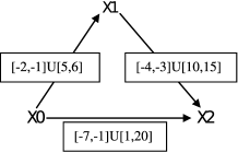
Figure 1: The network representation of the TCSP of Example 1.

Remark 1.

Let $(X_{i},X_{k},X_{j})$ be a triangle subnetwork of a TCSP $P$, with $|\mbox{mPcs}(C_{ij})|=n_{1}$, $|\mbox{mPcs}(C_{ik})|=n_{2}$ and $|\mbox{mPcs}(C_{kj})|=n_{3}$:

1. the worst-case computational complexity of the path-consistency operation, $C_{ikj}=C_{ij}\cap C_{ik}\otimes C_{kj}$, on triangle $(X_{i},X_{k},X_{j})$ is $O(n_{1}+n_{2}n_{3})=O(n_{2}n_{3})$;

2. the worst-case computational complexity of the weak path-consistency operation, $C_{ikj}=C_{ij}\cap C_{ik}\otimes_{w}C_{kj}$, on triangle $(X_{i},X_{k},X_{j})$ is $O(n_{1})$; and

3. if $C_{ij}$, $C_{ik}$ and $C_{kj}$ are convex, the worst-case computational complexity of both operations is $O(1)$.

See Appendix A for details.  

A distance graph is a complete labelled (weighted) directed graph $G=(V,E,w)$, where $V$ is the set of vertices (nodes), $E=V\times V$ is the set of edges, and $w$ is a labelling (weight) function from $E$ to the set ${\rm I\!R}\cup\{+\infty\}$ verifying $w(V_{i},V_{i})=0$, for all vertices $V_{i}$. A rooted distance graph is a pair $(G,S)$, where $G$ is a distance graph and $S$ is a vertex of G. A path of length $p$, or $p$-path, of a distance graph is a sequence $\pi=(V_{i_{0}},\cdots,V_{i_{p}})$ of vertices. The length of a path gives the number of its edges.

Let $\pi=(V_{i_{0}},\cdots,V_{i_{p}})$ be a $p$-path of a distance graph $G=(V,E,w)$. $\pi$ is elementary if, for all $j,k$ such that $\{j,k\}\not=\{0,p\}$, if $j\not=k$ then $V_{i_{j}}\not=V_{i_{k}}$; it is a circuit if $V_{i_{0}}=V_{i_{p}}$. The weight function $w$ of $G$ can be extended to paths as follows. The weight of $\pi$ is the sum $w(\pi)=\sum_{j=0}^{p-1}w(V_{i_{j}},V_{i_{j+1}})$. A (strictly) negative circuit is a circuit whose weight is strictly negative.

We now define the distance graph and the rooted distance graph of an STP.

Definition 14 ((rooted) distance graph of an STP).

If the TCSP $P=(X,C)$ is an STP, its distance graph is the distance graph $G=(X,X\times X,w)$ constructed as follows:

1. the set of vertices of $G$ is the set $X$ of variables of $P$

2. The labelling function $w$ is built as follows:

   1. for all variables $X_{i}$ and $X_{j}$, with $i<j$, if $P$ has a constraint $(X_{j}-X_{i})\in C_{ij}$, with $C_{ij}$ of the form $(-\infty,b]$, $[a,b]$ or $(a,b]$, then the label of edge $(X_{i},X_{j})$ is $b$: $w(X_{i},X_{j})=b$

   2. for all variables $X_{i}$ and $X_{j}$, with $i<j$, if $P$ has a constraint $(X_{j}-X_{i})\in C_{ij}$, with $C_{ij}$ of the form $(-\infty,b)$, $[a,b)$ or $(a,b)$, then the label of edge $(X_{i},X_{j})$ is $b^{-}$: $w(X_{i},X_{j})=b^{-}$

   3. for all variables $X_{i}$ and $X_{j}$, with $i<j$, if $P$ has a constraint $(X_{j}-X_{i})\in C_{ij}$, with $C_{ij}$ of the form $[a,+\infty)$, $[a,b]$ or $[a,b)$, then the label of edge $(X_{j},X_{i})$ is $-a$: $w(X_{j},X_{i})=-a$

   4. for all variables $X_{i}$ and $X_{j}$, with $i<j$, if $P$ has a constraint $(X_{j}-X_{i})\in C_{ij}$, with $C_{ij}$ of the form $(a,+\infty)$, $(a,b]$ or $(a,b)$, then the label of edge $(X_{j},X_{i})$ is $(-a)^{-}$: $w(X_{j},X_{i})=(-a)^{-}$

   5. all other edges $(X_{i},X_{j})$, with $i\not=j$, are such that $w(X_{i},X_{j})=+\infty$

We refer to the rooted distance graph $(G,X_{0})$ as the rooted distance graph of the STP $P$.  

Remark 2.

1. If an STP $P$ contains a constraint $(X_{j}-X_{i})\in[a,b)$, then, from Items 2b and 2c of Definition 14, the two edges $(X_{i},X_{j})$ and $(X_{j},X_{i})$ of the (rooted) distance graph of $P$ are labelled, respectively, with $b^{-}$ and $-a$. This is so because the constraint is equivalent to the following conjunction of linear inequalities: $X_{j}-X_{i}<b\wedge X_{i}-X_{j}\leq-a$. To have uniform linear inequalities, using exclusively $\leq$ (lower than or equal to), we write the inequality $X_{j}-X_{i}<b$ as $X_{j}-X_{i}\leq b^{-}$, the minus sign in $b^{-}$ meaning that the upper bound b is not reached. Note that if a distance graph contains an edge $(X,Y)$ labelled with $a$, with $a\in{\rm I\!R}\cup{\rm I\!R}^{-}$ and ${\rm I\!R}^{-}=\{a^{-}\mbox{ such that }a\in{\rm I\!R}\}$, this is interpreted as $Y-X\leq a$.

2. In order to be able to apply shortest paths algorithms to a (rooted) distance graph as defined in this work, the addition ($+$) and comparison ($<$) of real numbers should be generalised to ${\rm I\!R}\cup{\rm I\!R}^{-}$. This is done as follows, where $a,b\in{\rm I\!R}$:

   1. $a+b$ and $a<b$ are interpreted in the usual way;

   2. $a+b^{-}=a^{-}+b=a^{-}+b^{-}=(a+b)^{-}$;

   3. $a^{-}<a$; and

   4. if $a<b$ then $a^{-}<b$, $a<b^{-}$ and $a^{-}<b^{-}$.

   Of particular importance for the detection of negative circuits, $0^{-}<0$, meaning that $0^{-}$ is a (strictly) negative weight.  

Theorem 1 (Pratt (1977); Shostak (1981)).

Let $P$ be an STP. $P$ is consistent if and only if its distance graph has no negative circuit.  

The use of labelled directed graphs to represent a conjunction of linear inequalities, as used in Dechter et al. (1991), is restricted to large inequalities of the form $X_{j}-X_{i}\leq a$, where $a\in{\rm I\!R}$. An idea similar to the one used in this work, which combines large and strict inequalities, can be found in Kautz and Ladkin (1991).

Definition 15 (d-graph of an STP).

The d-graph of an STP $P=(X,C)$ is the distance graph $G=(X,X\times X,w)$ verifying: $w(X_{i},X_{j})$ is the weight of the shortest path from $X_{i}$ to $X_{j}$ in the distance graph of $P$.

The d-graph of an STP can be built from its distance gragh using Floyd-Warshall’s all-to-all shortest paths algorithm Aho et al. (1976); Papadimitriou and Steiglitz (1982).

Definition 16 (STP of a rooted distance graph).

Let $(G,V_{0})$ be a rooted distance graph, with $G=(V,V\times V,w)$ and $V=\{V_{0},V_{1},\ldots,V_{n}\}$. The STP of $(G,V_{0})$ is the STP $P=(X,C)$, with $X=\{X_{0},X_{1},\ldots,X_{n}\}$, constructed as follows:

1. Initialise $C$ to the empty set: $C=\emptyset$;

2. for all vertices $V_{i}$ and $V_{j}$ of $G$, with $i<j$, such that at least one of the two edges $(V_{i},V_{j})$ and $(V_{j},V_{i})$ is not labelled with $+\infty$:

   1. let $l_{1}=w(V_{i},V_{j})$ and $l_{2}=w(V_{j},V_{i})$;

   2. add to $C$ the constraint $(X_{j}-X_{i})\in M[l_{1},l_{2}]$, where $M[l_{1},l_{2}]$ is as given by the table $M$ of Figure 2 ($l_{1}$ of the form $+\infty$, $a$ or $a^{-}$, with $a\in{\rm I\!R}$; and $l_{2}$ of the form $+\infty$, $b$ or $b^{-}$, with $b\in{\rm I\!R}$).

For instance, if the edges $(V_{1},V_{5})$ and $(V_{5},V_{1})$ are labelled, respectively, with 6 and $(-2)^{-}$, the constraint $(X_{5}-X_{1})\in(2,6]$ is added to $C$.

In Dechter et al. (1991), it has been shown that applying path-consistency to an STP $P$ is equivalent to applying Floyd-Warshall’s all-to-all shortest paths algorithm Aho et al. (1976); Papadimitriou and Steiglitz (1982) to the distance graph of $P$. In other words, if $P^{\prime}$ is the STP resulting from applying path consistency to $P$ ($P^{\prime}=PC(P)$), then $P^{\prime}$ is exactly the STP of the d-graph of $P$. Furthermore, $P^{\prime}$ is minimal and strongly $n+1$-consistent, $n+1$ being the number of variables.

Theorem 2 (Dechter et al. (1991)).

Let $P$ be an $n+1$-variable STP. If path-consistency applied to $P$ does not detect an inconsistency, then the resulting STP $P^{\prime}$ is minimal and strongly $n+1$-consistent. Furthermore, $P^{\prime}$ is the STP of the d-graph of $P$.

$\begin{array}[]{|l|l||l|l|l|}\cline{3-5}\cr\lx@intercol\hbox{\multirowsetup}\hfil\lx@intercol\vrule\lx@intercol&\vrule\lx@intercol\hfil l_{2}\hfil\lx@intercol\vrule\lx@intercol\\ \cline{3-5}\cr\lx@intercol\hfil\lx@intercol\vrule\lx@intercol&+\infty&b&b^{-}\\ \hline\cr\cline{3-5}\cr\hbox{\multirowsetup$l_{1}$}&+\infty&(-\infty,+\infty)&[-b,+\infty)&(-b,+\infty)\\ \cline{2-5}\cr&a&(-\infty,a]&[-b,a]&(-b,a]\\ \cline{2-5}\cr&a^{-}&(-\infty,a)&[-b,a)&(-b,a)\\ \hline\cr\end{array}$

Figure 2: The table $M$ for the transformation of a rooted distance graph to an STP, with $a,b\in{\rm I\!R}$.

For the detection of an STP’s inconsistency, which is equivalent to the detection of a negative circuit in its distance graph Pratt (1977); Shostak (1981), we will need a lower bound of the weight of a finite-weight elementary path. Furthermore, for the purpose of evaluating the computational behaviour of the binarized-domains Arc-Consistency algorithm to be defined, we will additionaly need a upper bound of the same weight. These are defined as follows.

Definition 17 (path-lb, path-ub of an STP).

Let $P=(X,C)$ be an $n+1$-variable STP, $G=(X,X\times X,w)$ its rooted distance graph, and $Edges_{<}(P)$ and $Edges_{\geq}(P)$ the following subsets of $X\times X$:

1. $Edges_{<}(P)=\{(X_{i},X_{j}):\mbox{ }i\not=j\mbox{ and }w(X_{i},X_{j})<0\mbox{ and }w(X_{i},X_{j})<w(X_{j},X_{i})\}\cup\{(X_{i},X_{j}):\mbox{ }i<j\mbox{ and }w(X_{i},X_{j})<0\mbox{ and }w(X_{i},X_{j})=w(X_{j},X_{i})\}$,

2. $Edges_{\geq}(P)=\{(X_{i},X_{j}):\mbox{ }i\not=j\mbox{ and }0\leq w(X_{i},X_{j})<+\infty\mbox{ and }(w(X_{j},X_{i})=+\infty\mbox{ or }w(X_{j},X_{i})<w(X_{i},X_{j})\}\cup\{(X_{i},X_{j}):\mbox{ }i<j\mbox{ and }0\leq w(X_{i},X_{j})<+\infty\mbox{ and }w(X_{j},X_{i})=w(X_{i},X_{j})\}$.

We suppose that the elements of $Edges_{<}(P)$ (respectively, $Edges_{\geq}(P)$) are sorted in ascending (respectively, descending) order of their weights, and refer to the edge number $i$ as $Edges_{<}[P,i]$ (respectively, $Edges_{\geq}[P,i]$). $\mbox{path-lb}(P)$ and $\mbox{path-ub}(P)$ give, respectively, a lower bound and a upper bound of the weight of an elementary path of $P$, and are defined as follows:

$$\mbox{path-lb}(P)=\left\{\begin{aligned} 0\hskip 45.52458pt\mbox{ if }Edges_{<}(P)=\emptyset,\\ \Sigma_{(X,Y)\in Edges_{<}(P)}w(X,Y)\hskip 22.76228pt\\ \mbox{ if }|Edges_{<}(P)|\leq n,\\ \Sigma_{i=1}^{n}w(Edges_{<}[P,i])\mbox{ otherwise}\end{aligned}\right.$$

$$\mbox{path-ub}(P)=\left\{\begin{aligned} 0\hskip 45.52458pt\mbox{ if }Edges_{\geq}(P)=\emptyset,\\ \Sigma_{(X,Y)\in Edges_{\geq}(P)}w(X,Y)\hskip 22.76228pt\\ \mbox{ if }|Edges_{\geq}(P)|\leq n,\\ \Sigma_{i=1}^{n}w(Edges_{\geq}[P,i])\mbox{ otherwise}\end{aligned}\right.$$

Definition 18 (path-lb, path-ub of a TCSP).

Let $P=(X,C)$ be an $n+1$-variable TCSP: $\mbox{path-lb}(P)=\mbox{path-lb}(cc(P))$ and $\mbox{path-ub}(P)=\mbox{path-ub}(cc(P))$.

Theorem 3.

Let $P=(X,C)$ be an $n+1$-variable STP, $G=(X,X\times X,w)$ its distance graph, and $u=(X_{i_{1}},\ldots,X_{i_{p}})$ an elementary path of $G$ that is not a circuit. If the weight $w(u)$ of $u$ is finite then $\mbox{path-lb}(P)\leq w(u)\leq\mbox{path-ub}(P)$.

Proof : Let $u$ be an elementary path of $G$, of finite weight:

1. The lowest weight possible for $u$, when $|Edges_{<}(P)|\leq n$, correponds to the case when the edges of $u$ are exactly those in $Edges_{<}(P)$; and when $|Edges_{<}(P)|>n$, it corresponds to the case when the edges of $u$ are the first $n$ in $Edges_{<}(P)$. In both cases, the weight is equal to $\mbox{path-lb}(P)$.

2. The uppest weight possible for $u$, when $|Edges_{\geq}(P)|\leq n$, correponds to the case when the edges of $u$ are exactly those in $Edges_{\geq}(P)$; and when $|Edges_{\geq}(P)|>n$, it corresponds to the case when the edges of $u$ are the first $n$ in $Edges_{\geq}(P)$. In both cases, the weight is equal to $\mbox{path-ub}(P)$.  

3 A binarized-domains arc-consistency algorithm for TCSPs

The transformation of the unary constraints of a TCSP into binary constraints, after the addition of an ”origin of the world” variable $X_{0}$, makes the constraints of the TCSP become exclusively binary. In this work, we look at the constraints between the ”origin of the world” variable $X_{0}$ and the other variables as representing the (binarized) domains of these other variables. With this in mind, we define a notion of arc-consistency for TCSPs, which we will refer to as binarized-domains arc-consistency, or bdAC for short.

Definition 19 (binarized-domains arc-consistency).

Let $P$ be a TCSP. $P$ is said to verify the binarized-domains arc-consistency, or to be bdArc-Consistent for short, if for all all $i,j\in\{1,\ldots,n\}$, $i\not=j$, the following holds: $P_{0i}\subseteq P_{0j}\otimes P_{ji}$.

Said differently, $P$ is bdArc-Consistent if, for all $i,j\in\{1,\ldots,n\}$, $i\not=j$, the following holds: for all $(a_{0},a_{i})\in{\rm I\!R}^{2}$ such that $(a_{i}-a_{0})\in P_{0i}$, there exists $a_{j}\in{\rm I\!R}$ such that $(a_{j}-a_{0})\in P_{0j}$ and the instantiation $(X_{i},X_{j})=(a_{i},a_{j})$ satisfies the constraints, if any, on variables $X_{i}$ and $X_{j}$.

Definition 20.

Let $P$ be a TCSP, and $X_{i}$ and $X_{j}$ two variables of $P$. $X_{j}$ is reachable from $X_{i}$ if and only if there exists a finite-weight elementary path from $X_{i}$ to $X_{j}$ in the distance graph of $cc(P)$, the convex closure of $P$. $X_{j}$ is disconnected from $X_{i}$ if none of $X_{i}$ and $X_{j}$ is reachable from the other; $X_{j}$ is connected to $X_{i}$ otherwise. $P$ is connectd if $X_{0}$ is connected to each of the other variables.

The algorithm of Figure 4 takes as input a TCSP $P$, and does the following:

1. it makes $P$ bd-ArcConsistent, if at all possible,

2. if $P$ cannot be made bd-ArcConsistent then it is inconsistent, and the algorithm detects the inconsistency.

We refer to the algorithm as bdAC-3, for it is mainly an adaptation of Mackworth’s Mackworth (1977) well-known arc-consistency algorithm AC-3. bdAC-3 initialises a queue $Q$ to all pairs $(i,j)$ such that $i\not=0$, $j\not=0$, $i\not=j$ and $P$ contains a (binary) constraint on $X_{i}$ and $X_{j}$. Then it proceeds by taking in turn the pairs in $Q$ for propagation. When a pair $(k,m)$ is taken (and removed) from $Q$, bdAC-3 calls the procedure REVISE (Figure 3) which eventually updates $P_{0k}$, which represents the binarized domain of $X_{k}$, if it is not a subset of the composition $P_{0m}\otimes P_{mk}$. The main difference of bdAC-3 with Mackworth’s Mackworth (1977) AC-3 lies in line 4 of procedure REVISE, which guarantees termination of bdAC-3, and can be explained as follows, where the notations $lowerB(A)$ and $upperB(A)$, for a set $A\subseteq{\rm I\!R}$, refer, respectively, to the lower bound and upper bound of $A$:

1. If $P$ is an STP, $-lowerB(P_{0k})$ and $upperB(P_{0k})$ stand for the current values of the weights of the shortest paths from $X_{k}$ to $X_{0}$ and from $X_{0}$ to $X_{k}$, respectively, in the rooted distance graph of $P$. Those of the two that are finite should satisfy the conditions of Theorem 3. In other words, the algorithm should make sure that the evolution of the two weights makes none of them get below the lower bound $\mbox{path-lb}(P)$. Should the condition get violated, this would correspond to the detection of a negative circuit in the rooted distance graph of $P$, and bdAC-3 would terminate with a negative answer to the consistency problem of $P$.

2. If $P$ is a general TCSP, given that $\mbox{path-lb}(P)=\mbox{path-lb}(cc(P))$ and that $P$ is a refinement of its convex closure $cc(P)$, line 4 of procedure REVISE still applies.

If the REVISE procedure successfully updates $P_{0k}$, without making it become empty, the pairs $(i,k)$ such that $i\notin\{0,k,m\}$ and $P$ has a constraint on $X_{i}$ and $K_{k}$, reenter the queue $Q$ if they are no longer there. The algorithm terminates when a binarized domain becomes empty, or when the queue $Q$ becomes empty.

This leads us to the following Theorem.

Theorem 4.

Le $P$ be a TCSP. The bdAC-3 algorithm applied to $P$ terminates and, either detects inconsistency of $P$ or computes a bd-Arc Consistent TCSP equivalent to $P$.  

1. procedure $\mbox{REVISE}(i,j)${

2. DELETE=false;

3. $temp=P_{0i}\cap P_{0j}\otimes P_{ji}$;

4. if($temp\not=P_{0i}$){

5. if[$temp\not=\emptyset$ and $(lowerB(temp)>-\mbox{path-lb}(P)$

6. or $upperB(temp)<\mbox{path-lb}(P))]temp=\emptyset$;

7. $P_{0i}=temp$;$P_{i0}=temp^{\smile}$;

8. DELETE=true

9. }

10. return DELETE

11. }

Figure 3: The boolean procedure REVISE.

1. procedure $\mbox{bdAC-3}(P)${

2. $Q=\{(i,j):\mbox{ }P\mbox{ }has\mbox{ }a\mbox{ }constraint\mbox{ }on\mbox{ }X_{i}\mbox{ }and\mbox{ }X_{j},$

3. $\mbox{ }i*j\not=0,\mbox{ }i\not=j\}$;

4. $Empty\_domain=false$;

5. while $(Q\not=\emptyset$ and (not Empty_domain)){

6. select and delete an arc $(k,m)$ from $Q$;

7. if $\mbox{REVISE}(k,m)$

8. if $(P_{0k}=\emptyset)$ $Empty\_domain=true$

9. else $Q=Q\cup\{(i,k):\mbox{ $P$ has a constraint}$

10. on $X_{i}$ and $X_{k}$, $i\not=0$, $i\not=k$, $i\not=m$}

11. }%endwhile

12. return(not $Empty\_domain$)

13. }%end bdAC3

Figure 4: The binarized-domains Arc-Consistency algorithm bdAC-3.

The range of a TCSP will be needed for the determinination of the computational complexity of bdAC-3:

Definition 21 (range of a TCSP).

Let $P=(X,C)$ be an n+1-variable TCSP. The range of $P$, $rg(P)$, is defined as $rg(P)=\mbox{path-ub}(P)-\mbox{path-lb}(P)$.

Theorem 5.

Let $P=(X,C)$ be a TCSP, with $|X|=n+1$ and $|C|=m$. bdAC-3 applied to $P$ can be achieved in $O(n^{2}R)=O(mR)$ relaxation steps (calls of the procedure REVISE of Figure 3) and $O(n^{2}R^{3})=O(mR^{3})$ arithmetic operations, where $R=rg(P)$ is the range of $P$ expressed in the coarsest possible time units.

Proof: The worst case scenario of bdAC-3 occurs when, whenever the procedure REVISE updates $P_{0i}$, the length of the set $P_{0i}$ decreases by one time unit. Furthermore, if $P_{0i}$ has a finite bound, it will be in the set $[\mbox{path-lb}(P),\mbox{path-ub}(P)]$ (Theorem 3). Therefore, $P_{0i}$ can be updated at most $\mbox{path-ub}(P)-\mbox{path-lb}(P)=R=O(R)$ times. The pairs $(i,j)$ that enter initially the queue $Q$ of bdAC-3 are such that there is a constraint of $P$ on $X_{i}$ and $X_{j}$. A pair $(k,i)$ can reenter the queue $O(R)$ times, whenever $P_{0i}$ has been updated. Because there are $m=O(n^{2})$ constraints, the number of relaxation steps is $O(mR)=O(n^{2}R)$. A relaxation step consists of a call $\mbox{REVISE}(i,j)$ consisting mainly of the computation of a path consistency operation of the form $P_{0i}=P_{0i}\cap P_{0j}\otimes P_{ji}$, which needs $O(R^{2})$ arithmetic operations since each of the three sets $P_{0i}$, $P_{0j}$ and $P_{ji}$ is a union of at most $R$ convex subsets. The whole algorithm therefore terminates in $O(mR^{3})=O(n^{2}R^{3})$ time.  

For an STP, a relaxation step is in $O(1)$ (see Remark 1). This justifies the following corollary to Theorem 5.

Corollary 1.

Let $P=(X,C)$ be an STP, with $|X|=n+1$ and $|C|=m$. bdAC-3 applied to $P$ can be achieved in $O(n^{2}R)=O(mR)$ relaxation steps (calls of the procedure REVISE of Figure 3) and $O(n^{2}R)=O(mR)$ arithmetic operations, where $R=rg(P)$ is the range of $P$ expressed in the coarsest possible time units.  

Theorem 6.

Let $P$ be a connected STP (no variable $X_{i}$, $i>0$, is disconnected from $X_{0}$). If $P$ is bdArc-Consistent, its (binarized) domains are minimal: for all $i\in\{1,\ldots,n\}$, for all $a\in P_{0i}$, there exists a solution $(X_{0},X_{1},\ldots,X_{i},\ldots,X_{n})=(t_{0},t_{1},\ldots,t_{i},\ldots,t_{n})$ such that $t_{i}-t_{0}=a$.

Proof: Let $P$ be a connected bdArc-Consistent STP. Let $(G,X_{0})$ be the rooted distance graph of $P$, with $G=(X,X\times X,w)$. According to Theorem 2, showing that the binarized domains $P_{0i}$, with $i\in\{1,\ldots,n\}$, are minimal, is equivalent to showing that the labels (weights) $w(X_{0},X_{i})$ and $w(X_{i},X_{0})$ are the weights of the shortest paths from $X_{0}$ to $X_{i}$ and from $X_{i}$ to $X_{0}$, respectively. Suppose that this is not the case; in other words, that for some $i\in\{1,\ldots,n\}$, either $w(X_{0},X_{i})$ is not the weight of the shortest path from $X_{0}$ to $X_{i}$, or $w(X_{i},X_{0})$ is not the weight of the shortest path from $X_{i}$ to $X_{0}$:

1. Case 1: $w(X_{0},X_{i})$ is not the weight of the shortest path from $X_{0}$ to $X_{i}$. This would mean the existence of $j$ in $\{1,\ldots,n\}$, $j\not=i$, and of a path $<X_{i_{0}}=X_{0},X_{i_{1}}=X_{j},\ldots,X_{i_{k}}=X_{i}>$ from $X_{0}$ to $X_{i}$ through $X_{j}$, whose weight is strictly smaller than $w(X_{0},X_{i})$: $w(X_{i_{0}},X_{i_{1}})+w(X_{i_{1}},X_{i_{2}})+\cdots+w(X_{i_{k-1}},X_{i_{k}})<w(X_{i_{0}},X_{i_{k}})$. But, because the STP is bdArc-Consistent, we have the following:

   $$\left\{\begin{aligned} w(X_{i_{0}},X_{i_{2}})&\leq&w(X_{i_{0}},X_{i_{1}})+w(X_{i_{1}},X_{i_{2}})\\ w(X_{i_{0}},X_{i_{3}})&\leq&w(X_{i_{0}},X_{i_{2}})+w(X_{i_{2}},X_{i_{3}})\\ \cdots&\cdots&\cdots\\ w(X_{i_{0}},X_{i_{k}})&\leq&w(X_{i_{0}},X_{i_{k-1}})+w(X_{i_{k-1}},X_{i_{k}})\end{aligned}\right.$$

   Summing the left-hand sides and the right-hand sides of the linear inequalities, we get: $w(X_{i_{0}},X_{i_{k}})+\displaystyle\Sigma_{l=2}^{k-1}w(X_{i_{0}},X_{i_{l}})\leq w(X_{i_{i_{0}}},X_{i_{1}})+w(X_{i_{1}},X_{i_{2}})+\cdots+w(X_{i_{k-1}},X_{i_{k}})+\displaystyle\Sigma_{l=2}^{k-1}w(X_{i_{0}},X_{i_{l}})$. This, in turn, gives $w(X_{i_{0}},X_{i_{k}})\leq w(X_{i_{i_{0}}},X_{i_{1}})+w(X_{i_{1}},X_{i_{2}})+\cdots+w(X_{i_{k-1}},X_{i_{k}})$, which clearly contredicts our supposition.

2. Case 2: $w(X_{i},X_{0})$ is not the weight of the shortest path from $X_{i}$ to $X_{0}$. This would mean the existence of $j$ in $\{1,\ldots,n\}$, $j\not=i$, and of a path $<X_{i_{0}}=X_{i},X_{i_{1}}=X_{j},\ldots,X_{i_{k}}=X_{0}>$ from $X_{i}$ to $X_{0}$ through $X_{j}$, whose weight is strictly smaller than $w(X_{i},X_{0})$: $w(X_{i_{0}},X_{i_{1}})+w(X_{i_{1}},X_{i_{2}})+\cdots+w(X_{i_{k-1}},X_{i_{k}})<w(X_{i_{0}},X_{i_{k}})$. But, because the STP is bdArc-Consistent, we have the following:

   $$\left\{\begin{aligned} w(X_{i_{0}},X_{i_{k}})&\leq&w(X_{i_{0}},X_{i_{1}})+w(X_{i_{1}},X_{i_{k}})\\ w(X_{i_{1}},X_{i_{k}})&\leq&w(X_{i_{1}},X_{i_{2}})+w(X_{i_{2}},X_{i_{k}})\\ \cdots&\cdots&\cdots\\ w(X_{i_{k-2}},X_{i_{k}})&\leq&w(X_{i_{k-2}},X_{i_{k-1}})+w(X_{i_{k-1}},X_{i_{k}})\end{aligned}\right.$$

   Summing the left-hand sides and the right-hand sides of the linear inequalities, we get: $w(X_{i_{0}},X_{i_{k}})+\displaystyle\Sigma_{l=1}^{k-2}w(X_{i_{l}},X_{i_{k}})\leq w(X_{i_{0}},X_{i_{1}})+w(X_{i_{1}},X_{i_{2}})+\cdots+w(X_{i_{k-1}},X_{i_{k}})+\displaystyle\Sigma_{l=1}^{k-2}w(X_{i_{l}},X_{i_{k}})$. This, in turn, gives $w(X_{i_{0}},X_{i_{k}})\leq w(X_{i_{0}},X_{i_{1}})+w(X_{i_{1}},X_{i_{2}})+\cdots+w(X_{i_{k-1}},X_{i_{k}})$, which clearly contredicts our supposition.  

As an immediate consequence of Theorem 6:

Corollary 2.

Let $(G,V)$ be a rooted distance graph. The bdArc-Consistency algorithm bdAC-3 can be used to compute the weights of the shortest paths from $V$ to all vertices of $G$, and the weights of the shortest paths from all vertices of $G$ to $V$.

Proof. Proceed as follows:

1. Linearly transform the input rooted distance graph $(G,V)$ into its STP $P$;

2. apply the bdArc-Consistency algorithm bdAC-3 to $P$;

3. linearly transform the STP resulting from bdAC-3 into its rooted distance graph.  

Appendices B and C present two detailled examples. The example of Appendix B applies the bdAC-3 algorithm to an STP, transforming the latter into a bdArc-Consistent STP with no variable disconnected from the ”origin of the world” variable, without making a binarized domain become empty. The example of Appendix C applies bdAC-3 to an STP whose rooted distance graph presents a negative circuit not reachable from $X_{0}$, the ”origin of the world” variable, but from which $X_{0}$ is reachable: bdAC-3 detects the negative circuit, and the inconsistency of the STP. In particular, the example of Appendix C shows that bdAC-3 without line 4 of procedure REVISE, which could be seen as a ”literal” adaptation to TCSPs of Mackworth’s Mackworth (1977) algorithm AC-3, has no guarantee to always terminate (see Remark 3).

Remark 3.

We refer to the procedure REVISE of Figure 3 without its line 4 as $\mbox{REVISE}^{-}$, and to the algorithm bdAC-3 (Figure 4) in which procedure REVISE is replaced with $\mbox{REVISE}^{-}$ as $\mbox{bdAC-3}^{-}$. $\mbox{bdAC-3}^{-}$ is, somehow, a ”literal” adaptation of Mackworth’s Mackworth (1977) AC-3 algorithm to TCSPs. In the light of the example of Appendix C, $\mbox{bdAC-3}^{-}$ is not guaranteed to always terminate.

4 Consistency of a bdArc-Consistent STP: a backtrack-free procedure

Given a bdArc-Consistent STP $P$, the backtrack-free procedure $connectX0\_in\_bdACstp(P)$ of Figure 5 checks consistency of $P$: it extracts a connected bdArc-Consistent STP refinement of $P$, and returns true, if $P$ consistent; it returns false otherwise. Correctness of procedure $connectX0\_in\_bdACstp(P)$ is guaranteed by Theorem 7.

Theorem 7.

Let $P=(X,C)$ be a bdArc-Consistent STP with a variable $X_{i}$, $i\geq 1$, disconnected from $X_{0}$, and $P^{\prime}=(X,C\cup\{(X_{i}-X_{0})\in[a,+\infty)\})$ the STP obtained from $P$ by adding the constraint $(X_{i}-X_{0})\in[a,+\infty)$, with $a\in{\rm I\!R}$. $P$ is consistent if and only if $P^{\prime}$ is consistent.

Proof: Immediate consequence of Theorem 1 and the fact that the rooted distance graphs of $P$ and $P^{\prime}$ are such that one has a negative circuit if and only if the other has.  

1. Input: The matrix representation of a bdArc-Consistent STP $P$ having variables disconnected from $X_{0}$.

2. Output: Extracts a connected bdArc-Consistent STP refinement of $P$, and returns true, if $P$ consistent; returns false otherwise.

3. procedure $connectX0\_in\_bdACstp(P)${

1. select a variable $X_{i}$ disconnected from $X_{0}$, and a real number $a$;

2. $P_{0i}=[a,+\infty)$; $P_{i0}=(-\infty,-a]$;

3. if($\mbox{bdAC-3}(P)$)

4. if ($P$ has no variable disconnected from $X_{0}$)

5. return true

6. else $connectX0\_in\_bdACstp(P)$

7. else return false

8. }

Figure 5: The polynomial backtrack-free procedure $connectX0\_in\_bdACstp(P)$.

5 Searching for a solution of a connected bdArc-Consistent STP: a backtrack-free procedure

1. Input: The matrix representation of a bdArc-Consistent STP $P$ with no variable disconnected from $X_{0}$.

2. Output: A bdArc-Consistent singleton-domains STP refinement of $P$.

3. procedure $backtrack\_free(P)${

4. if($P$ has non-singleton binarized domains){

5. select a non-singleton edge $(X_{0},X_{i})$;

6. Instantiate $(X_{0},X_{i})$ with an element $a_{i}$ of $P_{0i}$:

7. $P_{0i}=\{a_{i}\};P_{i0}=\{-a_{i}\}$;

8. $P=\mbox{bdAC-3}(P)$;

9. $backtrack\_free(P)$}%endif

10. else return $P$

11. }

Figure 6: A polynomial backtrack-free procedure computing a consistent singleton refinement of a connected bdArc-Consistent STP.

Correctness of the backtrack-free procedure of Figure 6 is a direct consequence of Theorem 6. If the input bdArc-Consistent STP $P$ is not a singleton STP (line 1), we select a non-singleton edge $(X_{0},X_{i})$ and instantiate it with an element $a_{i}$ of $P_{0i}$ (lines 2 and 3): because $P$ is connected and bdArc-Consistent, the binarized domain $P_{0i}$ is minimal (Theorem 6), which guarantees that the element $a_{i}$ chosen to instantiate edge $(X_{0},X_{i})$ participates in a global solution. bdArc-Consistency is then applied to the refinement resulting from the instantiation (line 4). The process needs to be reiterated at most $n$ times before the binarized domains $P_{0i}$, $i\in\{1,\ldots,n\}$, become singleton (line 6).

6 wbdAC-3 as the filtering procedure of a TCSP solver

1. procedure $consistent(P)${

2. if(not wbdAC-3$(P)$)return false

3. else

4. if($P$ has disjunctive edges){%beginif2

5. select a disjunctive edge $(X_{i},X_{j})$;

6. let $\mbox{mPcs}(P_{ij})=\{P_{ij_{1}},\ldots,P_{ij_{n_{ij}}}\}$;

7. for($k=1\mbox{ to }n_{ij}$){

8. $P^{\prime}=P$; $P_{ij}^{\prime}=P_{ij_{k}}$; $P_{ji}^{\prime}=P_{ij_{k}}^{\smile}$;

9. if($consistent(P^{\prime})$)return true}%endfor

10. return false}%endif2

11. else

12. if ($P$ has no variable disconnected from $X_{0}$)

13. return true

14. else return $connectX0\_in\_bdACstp(P)$

15. }

Figure 7: The recursive procedure $consistent(P)$.

We define a refinement of a TCSP $P$ to be any TCSP $P^{\prime}$ on the same set of variables such that for all constraint $(X_{j}-X_{i})\in P_{ij}^{{}^{\prime}}$ of $P^{\prime}$, the corresponding constraint $(X_{j}-X_{i})\in P_{ij}$ of $P$ verifies $P_{ij}^{{}^{\prime}}\subseteq P_{ij}$. A constraint $(X_{j}-X_{i})\in P_{ij}^{{}^{\prime}}$ such that $P_{ij}^{{}^{\prime}}\subseteq P_{ij}$ is called sublabel of $(X_{j}-X_{i})\in P_{ij}$. A refinement is convex if it is an STP Dechter et al. (1991). The solver can now be described as follows (see Figure 7). As the filtering procedure during the search, it uses a weak version of the bdArc-Consistency algorithm bdAC-3, which we refer to as wbdAC-3, and consists of replacing composition by weak composition in the REVISE procedure of Figure 3, the aim being to avoid the “fragmentation problem” Schwalb and Dechter (1997). If $P$ is the input TCSP, the recursive procedure $consistent(P)$ is called, which works as follows. The filtering procedure wbdAC-3 is applied (the very first application of the filtering, at the root of the search space, consists of the preprocessing step). If the wbdAC-3 filtering detects an inconsisteny (line 1), by reducing a binarized domain to the empty set, a failure (dead end) is reached and the procedure returns false. Otherwise, if $P$ has no disjunctive edge (line 10) then the result of the wbdAC-3 filtering is a bdArc-Consistent STP, which is not necessarily consistent since it might contain a negative circuit disconnected from $X_{0}$; and, in this case, the procedure does the following:

1. if $P$ has no variable disconnected from $X_{0}$ then $P$ is consistent (Theorem 6), and the procedure returns true (line 11);

2. if $P$ has variables that are disconnected from $X_{0}$ (line 12), these might hide a negative circuit, of which $X_{0}$ cannot be a vertex. The backtrack-free search procedure $connectX0\_in\_bdACstp(P)$ is called, which checks consistency of $P$: $consistent(P)$ returns the result returned by $connectX0\_in\_bdACstp(P)$.

If the result of the wbdAC-3 filtering is not an STP then there remain disjunctive edges (line 3). A disjunctive edge is selected (lines 4 and 5) and instantiated with one of its maximal convex sublabels (line 7): $P^{\prime}$ is the refinement of $P$ resulting from the instantiation. The recursive call $consistent(P^{\prime})$ is then made (line 8). If $consistent(P^{\prime})$ returns true, $consistent(P)$ returns true. If now $consistent(P^{\prime})$ returns false, the next maximal convex sublabel, if any, of the edge being instantiated is chosen, and the recursive call $consistent(P^{\prime})$ is made again. If all sublabels have been already chosen (line 9) then $consistent(P)$ returns false. Completeness of the solver is guaranteed by completeness of bdArc-Consistency for connected STPs (Theorem 6).

Given an input TCSP $P$, the solver of Figure 7 can be adapted so that, when $P$ is consistent, it returns a connected bdArc-Consistent STP refinement $P^{\prime}$ of $P$. From $P^{\prime}$, one can then get a solution to $P$ with the use of the polynomial backtrack-free procedure of Figure 6.

The next section describes how, from the general TCSP solver, one can extract a TCSP-based job shop scheduler with bdAC-3 as the filtering procedure during the search.

7 bdAC-3 as the filtering procedure of a TCSP-based job shop scheduler

1. Input: The matrix representation of a scheduling TCSP $P$.

2. Output: The optimum $z$ of $P$.

3. Method: Initialise the optimum: $z=+\infty$; then call the recursive procedure $optimum(P)$

4. procedure $optimum(P)${

5. if (not bdAC-3$(P)$ or $z\leq OLB(P))$ return

6. else

7. if($P$ has disjunctive edges){%beginif2

8. select a disjunctive edge $(X_{i},X_{j})$;

9. let $A=P_{ij}=A_{1}\cup A_{2}$;

10. for($k=1\mbox{ to }2$){

11. $P^{\prime}=P$; $P_{ij}=A_{k}$; $P_{ji}=A_{k}^{\smile}$;

12. $optimum(P^{\prime})$}%endfor

13. }%endif2

14. else update($z$): $z=OLB(P)$

15. }

Figure 8: The TCSP-based job-shop scheduler.

Many approaches to scheduling are known in the literature, among which mathematical programming, timed Petri nets Carlier et al. (1985) and discrete CSPs Dincbas et al. (1990); Sadeh et al. (1995). We focus on job shop scheduling problems.

A scheduling TCSP is a TCSP $P=(X,C)$, with $X=\{X_{0},X_{1},\ldots,X_{n}\}$, $X_{0}$ being the ”origin of the world” variable standing for a global release date, $n$ being the number of (non-preemptive) tasks:

1. For $i\in\{1,\ldots,n\}$:

   1. variable $X_{i}$ stands for the starting date of task $i$;

   2. the duration of task $i$ is $d_{i}$, with $d_{i}>0$ (the tasks are durative, in the sense that their durations are not null; furthermore, they have fixed durations, known in advance); and

   3. the release and due dates of task $i$, if any, are $rd_{i}$ and $dd_{i}$.

2. A conjunctive (or precedence) constraint between tasks $i$ and $j$ has the form $(X_{j}-X_{i})\in[d_{i},+\infty)$.

3. A disjunctive constraint between tasks $i$ and $j$ has the form $(X_{j}-X_{i})\in(-\infty,-d_{j}]\cup[d_{i},+\infty)$.

4. A release (respectively, due) date constraint has the form $(X_{i}-X_{0})\in[rd_{i},+\infty)$ (respectively, $(X_{i}-X_{0})\in[0,dd_{i}-d_{i}]$).

5. Finally, $X_{0}$ standing for a global release date, we add the $n$ constraints $(X_{i}-X_{0})\in[0,+\infty)$, $i\in\{1,\ldots,n\}$.

We define the duration $dur(s)$ of a solution $s=(X_{0}=t_{0},X_{1}=t_{1},\ldots,X_{n}=t_{n})$ of $P$ as $dur(s)=\displaystyle max_{i=1}^{n}(t_{i}+d_{i})-t_{0}$; the latency $lat(s)$ of $s$ as the amount of time separating stimulus and response, the stimulus being given at time $t_{0}$, and the response obtained at the effective beginning of the very first task: $lat(s)=\displaystyle min_{i=1}^{n}t_{i}-t_{0}$. The optimum of $P$, $t_{opt}^{P}$, is defined as $t_{opt}^{P}=\displaystyle min_{s\in sol(P)}dur(s)$, with $sol(P)$ being the set of solutions of $P$. The scheduler we propose (Figure 8), with bdAC-3 as the filtering procedure during the search, minimises the makespan and initialises the optimum $z$ to $+\infty$; it is an adaptation of the TCSP solver of Figure 7. The lower bound of the optimum of $P$, $OLB(P)$, is defined as $OLB(P)=\displaystyle max_{i=1}^{n}(a_{i}+d_{i})$, where $a_{i}$ is the lower bound of the binarized domain $P_{0i}$. Note that $t_{opt}^{P}\leq OLB(P)$, which is used by the scheduler to backtrack whenever $z\leq OLB(P)$ (line 1). Furthermore, whenever the bdAC-3 filtering leads to a (bdArc-Consistent) STP (line 10), the optimum is updated in a way one can justify as follows. Given the nature of a scheduling TCSP ($X_{0}$ is a global release date), $X_{0}$ is disconnected from none of the other variables. Because the binarized domains $P_{0i}$ of a connected bdArc-Consistent STP $P$ are minimal (Theorem 6), a direct consequence of results in Dechter et al. (1991) (Corollaries 3.2 and 3.4, Pages 69 and 70) is that the solution realising the optimum of $P$ is given by the lower bounds of these binarized domains, and the optimum itself is $OLB(P)$. See Figure 8 for details.

The relaxation step of the bdAC-3 algorithm, consisting of a call of the $\mbox{REVISE}(i,j)$ procedure of Figure 3, and reducing mainly to the path-consistency operation $P_{0i}=P_{0i}\cap P_{0j}\otimes P_{ji}$, may result in a fragmentation of the binarized domain $P_{0i}$, as illustrated by Example 1. To avoid such a fragmentation, we used in the general TCSP solver of Section 6, a weak version of the bdAC-3 algorithm, wbdAC-3, as the filtering procedure.

The restriction to scheduling TCSPs, however, makes it possible to use bdAC-3 as the filtering procedure, with no risk of fragmenting a binarized domain. Given such a TCSP $P=(X,C)$, with $X=\{X_{0},X_{1},\ldots,X_{n}\}$, the binarized domains $P_{0i}$, with $i\in\{1,\ldots,n\}$, are of either of the two forms $[a,b]$ (form A1) or $[a,+\infty)$ (form A2), with $0\leq a\leq b$. Furthermore, the entries $P_{ij}$ of the matrix representation of $P$, with $i*j\not=0$ and such that there is a constraint on tasks $i$ and $j$, are of either of the three forms $(-\infty,a]$ with $a<0$ (form B1), $[a,+\infty)$ with $a>0$ (form B2), or $(-\infty,a]\cup[b,+\infty)$ with $a<0<b$ (form B3). Therefore, the composition $P_{0j}\otimes P_{ji}$ of the $\mbox{REVISE}(i,j)$ procedure of Figure 3 results in a convex set with no open finite bound; this implies that, the relaxation operation $P_{0i}=P_{0i}\cap P_{0j}\otimes P_{ji}$ of the same procedure, replacing the binarized domain $P_{0i}$ with its intersection with the composition $P_{0j}\otimes P_{ji}$, results in a binarized domain of either of the two forms A1 or A2. This leads to the following theorem:

Theorem 8.

The class of scheduling TCSPs is closed under bdArc-Consistency: applying a bdArc-Consistency algorithm, such as bdAC-3, to a schedulig TCSP $P$ either detects inconsistency of $P$, or computes an (equivalent, bdArc-Consistent) scheduling TCSP.  

Theorem 8 justifies our use of bdAC-3 as the filtering procedure of our TCSP-based scheduler, instead of its weak version wbdAC-3: bdAC-3 applied to a scheduling TCSP does not fragment the binarized domains. Furthermore, given that the instantiation of a disjunctive edge transforms a constraint of the form B3 into a constraint of either of the two forms B1 and B2, the resulting refinement is a scheduling TCSP. This brings us to this nice behavior of the class of scheduling TCSPs: at each node of the scheduler’s search tree, the bdAC-3 filtering either detects inconsistency of the corresponding refinement, indicating a failure (deadend), or computes an (equivalent, bdArc-Consistent) scheduling TCSP.

8 Related work

Related work on arc-consistency for TCSPs include Cervoni et al. (1994); Cesta and Oddi (1996); Kong et al. (2018); Planken et al. (2008), but the focus has always been restricted to STPs. The most related remains Kong et al. (2018), which defines an arc-consistency algorithm for STPs, which can be seen as an adaptation of Bellman-Ford-Moore one-to-all shortest paths algorithm Bellman (1958); Ford and Fulkerson (1962); Moore (1959); this can also be seen as an adaptation of Mackworth’s Mackworth (1977) arc-consistency algorithm AC-1 restricted to one pass. Beyond the fact that the algorithm is defined only for STPs, the other criticism is that for applications needing incrementality such as planning, which seems to have been the authors’ targetted application, it is clear that the use of an adaptation of Mackworth’s Mackworth (1977) AC-3 instead of AC-1, in case of arc-consistency, and an adaptation of Mackworth’s Mackworth (1977) PC-2 instead of PC-1, in case of path-consistency, is much better, mainly because these use a queue allowing them, when new knowledge comes in, to continue on what had been done before, and not to redo it. Allen’s well-known Interval Algebra Allen (1983) in general, and its convex part in particular, whose most targetted application is planning, uses an adaptation of PC-2.

The most related work, worth comparing, is Decther et al.’s Dechter et al. (1991), where, in particular, the authors show the equivalence between, on one hand, applying path-consistency to an STP and, on the other, applying an all-to-all shortest paths algorithm, such as Floyd-Warshall’s Aho et al. (1976); Papadimitriou and Steiglitz (1982), to the corresponding distance graph. Dechter et al. Dechter et al. (1991), as explained in the introduction, didn’t focus on node- and arc-consistencies, because the adding of an ”origin of the world” variable led them to the conclusion that a TCSP was already node- and arc-consistent. In the present work, we have looked at the constraints between the ”origin of the world” variable and the other variables, as the binarized domains of these other variables. This led us to the definition of the notion of binarized-domains Arc-Consistency, which is computationally one factor less expensive. We showed, in particular, that applying bdArc-Consistency to an STP was equivalent to applying a one-to-all all-to-one shortest paths algorithm to the corresponding rooted distance graph. The bdArc-Consistency algorithm we have defined, bdAC-3, detects negative circuits reachable from $X_{0}$, or from which $X_{0}$ is reachable.

Another related work is Schwalb and Dechter’s Schwalb and Dechter (1997), where, in particular, the authors propose the use of weak versions of path-consistency as filtering procedures of general TCSP solvers. One of these weaker versions is ULT (Upper-Lower Tightning), in which composition is replaced with weak composition. We have discussed the use of a similar idea in a general TCSP solver with the filtering procedure consisting of a weak version of the binarized-domains Arc-Consistency algorithm bdAC-3 proposed in this work.

The rest of the section presents an adaptation to TCSPs of the other local-consistency algorithms in Mackworth (1977), namely, the arc-consistency algorithm AC-1, and the path consistency algorithms PC-1 and PC-2; it also looks at the termination of these adaptations; and shows, in particular, that an existing adaptation to TCSPs of PC-2 Dechter et al. (1991); Schwalb and Dechter (1997) is not guaranteed to always terminate.

8.1 Adaptation to TCSPs of AC-1, PC-1 and PC-2

In addition to the bdAC-3 algorithm, we provide in Figures 9 and 10 adaptations to TCSPs of the other three local-consistency algorithms in Mackworth (1977): the arc-consistency algorithm AC-1 and the two path-consistency algorithms PC-1 and PC-2. The adaptations are named, respectively, bdAC-1, PC-1 and PC-2. Like bdAC-3, when applied to an STP, bdAC-1 detects, if any, negative circuits reachable from $X_{0}$, or from which $X_{0}$ is reachable, in the corresponding rooted distance graph; it makes the STP bdArc-Consistent otherwise. PC-1 and PC-2, when applied to an STP, both detect, if any, negative circuits in the corresponding distance graph; they make the STP path-consistent otherwise. Both of bdAC-1 and PC-2 use the condition on negative circuits one can extract from Theorem 3 (line 4 of the REVISE procedure of Figure 3, for bdAC-1; line 4 of the REVISE_PC-2 procedure of Figure 10, for PC-2).

1. Input: The matrix representation of a TCSP $P$.

2. Output: True, indicating that the TCSP has been made bdArc-consistent; or false, indicating that inconsistency of $P$ has been detected.

3. procedure $\mbox{bdAC-1}(P)${

4. $Q=\{(i,j):\mbox{ }P\mbox{ }has\mbox{ }a\mbox{ }constraint\mbox{ }on\mbox{ }X_{i}\mbox{ }and\mbox{ }X_{j},$

5. $\mbox{ }i*j\not=0,\mbox{ }i\not=j\}$;

6. repeat

7. CHANGE=false;

8. for each $(i,j)\in Q$

9. if $\mbox{REVISE}(i,j)${%begin if1

10. if($P_{0i}=\emptyset$)return false;

11. CHANGE=true

12. }%end if1

13. until $\neg$CHANGE

14. return true

15. }%end bdAC1

1. Input: The matrix representation of a TCSP $P$.

2. Output: True, indicating that the TCSP has been made path-consistent; or false, indicating that inconsistency of $P$ has been detected.

3. procedure $\mbox{PC-1}(P)${

4. repeat

5. CHANGE=false;

6. for ($k=0$ to $n$)

7. for ($i,j=0$ to $n$){

8. $temp=P_{ij}\cap P_{ik}\otimes P_{kj}$;

9. if($temp=\emptyset$)return false;

10. if($temp\not=P_{ij}$){$P_{ij}=temp$;CHANGE=true}

11. }

12. until $\neg$CHANGE

13. return true

14. }%end PC1

Figure 9: The binarized-domains Arc-Consistency algorithm bdAC-1 and the Path-Consistency algorithm PC-1.

1. procedure $\mbox{REVISE\_PC-2}(i,k,j)${

2. DELETE=false;

3. $temp=P_{ij}\cap P_{ik}\otimes P_{kj}$;

4. if($temp\not=P_{ij}$){

5. if[$temp\not=\emptyset$ and $(lowerB(temp)>-\mbox{path-lb}(P)$

6. or $upperB(temp)<\mbox{path-lb}(P))]temp=\emptyset$;

7. $P_{ij}=temp$;$P_{ji}=temp^{\smile}$;

8. DELETE=true

9. }

10. return DELETE

11. }

1. Input: The matrix representation of a TCSP $P$.

2. Output: True, indicating that the TCSP has been made path-consistent; or false, indicating that inconsistency of $P$ has been detected.

3. procedure $\mbox{PC-2}(P)${

4. $Q=\{(i,k,j):\mbox{ }(i<j)\mbox{ and }(k\notin\{i,j\})\mbox{ and}$

5. $(P_{ik}\subset{\rm I\!R})\mbox{ and }(P_{kj}\subset{\rm I\!R})\}$;

6. $Empty\_domain=false$;

7. while $(Q\not=\emptyset$ and (not Empty_domain)){

8. select and delete a triple $(i,k,j)$ from $Q$;

9. if $\mbox{REVISE\_PC-2}(i,k,j)$

10. if $(P_{ij}=\emptyset)$ $Empty\_domain=true$

11. else $Q=Q\cup$

12. $\{(i,j,m):\mbox{ $(i<m)$ and $(m\not=j)$ and $P_{jm}\subset{\rm I\!R}$}\}\cup$

13. $\{(m,i,j):\mbox{ $(m<j)$ and $(m\not=i)$ and $P_{mi}\subset{\rm I\!R}$}\}$

14. } %endwhile

15. return(not $Empty\_domain$)

16. } %end PC2

Figure 10: The path-consistency algorithm PC-2 and the boolean procedure REVISE_PC-2 it makes use of.

As already stated in Remark 3, we refer to the procedure REVISE of Figure 3 without its line 4 as $\mbox{REVISE}^{-}$, and to the algorithm bdAC-3 (Figure 4) in which procedure REVISE is replaced with $\mbox{REVISE}^{-}$ as $\mbox{bdAC-3}^{-}$. In addition to that, we refer to the procedure REVISE_PC-2 of Figure 10 without its line 4 as $\mbox{REVISE\_PC-2}^{-}$, to the algorithm bdAC-1 (Figure 9) in which procedure REVISE is replaced with $\mbox{REVISE}^{-}$ as $\mbox{bdAC-1}^{-}$, and to the algorithm PC-2 (Figure 10) in which procedure REVISE_PC-2 is replaced with $\mbox{REVISE\_PC-2}^{-}$ as $\mbox{PC-2}^{-}$.

8.2 Termination of the adaptations

PC-1 proceeds by passes, and each pass considers all possible triples of variables. It is a ”literal” adaptation from Mackworth (1977), and is guaranteed to terminate and to detect, when applied to an STP, the presence of negative circuits in the corresponding distance graph. This is not the case for $\mbox{bdAC-1}^{-}$ and $\mbox{PC-2}^{-}$, which, deprived of line 4 of Procedure REVISE for the former, and of line 4 of Procedure REVISE_PC-2 for the latter, have no guarantee to terminate even when the input is an STP. Example 2 shows that $\mbox{bdAC-1}^{-}$ and $\mbox{PC-2}^{-}$, which are ”literal” adaptations of Mackworth’s Mackworth (1977) AC-1 and PC-2, respectively, are not guarateend to terminate.

Example 2 (non termination of $\mbox{bdAC-1}^{-}$ and $\mbox{PC-2}^{-}$).

We consider the STP $P=(X,C)$ with:

1. $X=\{X_{0},X_{1},X_{2},X_{3}\}$ and

2. $C=\{c_{1}:(X_{1}-X_{0})\in[30,+\infty),c_{2}:(X_{2}-X_{1})\in[-20,-10],c_{3}:(X_{3}-X_{1})\in(-\infty,4],c_{4}:(X_{3}-X_{2})\in[40,50]\}$.

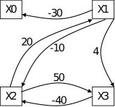
Figure 11: The distance graph of the STP of Example 2.

The rooted distance graph of $P$ (see Figure 11) does have a negative ciruit that is not reachable from $X_{0}$, but from which $X_{0}$ is reachable. bdAC-1 and $\mbox{bdAC-1}^{-}$ proceed by passes, each of which is guaranteed to terminate since it considers at most once each ordered pair $(X_{i},X_{j})$ such that there is a constraint on $X_{i}$ and $X_{j}$. Each of the two versions of bdArc-Consistency terminates when, either a binarized domain becomes empty, or a whole pass makes no change in the binarized domains. But for the version $\mbox{bdAC-1}^{-}$, the order in which the pairs in its queue are propagated might make it impossible for the two terminating conditions to occur. Initially, the binarized domains are as follows: $P_{01}=[30,+\infty)$, $P_{02}={\rm I\!R}$ and $P_{03}={\rm I\!R}$. For each of the two versions, we suppose that each of its passes propagates the pairs on which there is a constraint in the order $(X_{1},X_{2})$, $(X_{1},X_{3})$, $(X_{2},X_{1})$, $(X_{2},X_{3})$, $(X_{3},X_{1})$, $(X_{3},X_{2})$. For both versions, the evolution of the binarized domains for the first three passes are as follows:

1. after Pass 1: $P_{01}=[30,+\infty)$, $P_{02}=[10,+\infty)$ and $P_{03}=[50,+\infty)$

2. after Pass 2: $P_{01}=[46,+\infty)$, $P_{02}=[26,+\infty)$ and $P_{03}=[66,+\infty)$

3. after Pass 3: $P_{01}=[62,+\infty)$, $P_{02}=[42,+\infty)$ and $P_{03}=[82,+\infty)$

This means that each pass increases the (finite) lower bound of each binarized domain by 16, which corresponds to the absolute value of the weight of the negative circuit $(X_{1},X_{3},X_{2},X_{1})$. Given that $\mbox{path-lb}(P)=-80$, bdAC-1 will detect the negative circuit after the third pass. However, $\mbox{bdAC-1}^{-}$ will fail to do so, and will not terminate.

Let’s now look at how the two adaptations PC-2 and $\mbox{PC-2}^{-}$ of Mackworth’s Mackworth (1977) PC-2 will behave on the STP. Keep in mind that their unique difference lies in line 4 of Procedure REVISE_PC-2, which is absent in $\mbox{PC-2}^{-}$. Both versions will initialise their queue as follows: $Q=\{(X_{0},X_{1},X_{2}),(X_{0},X_{1},X_{3}),(X_{1},X_{2},X_{3})\}$. We take the triple $(X_{0},X_{1},X_{2})$ for propagation. The resulting modifications are as follows:

1. $P_{02}=[10,+\infty)$, $P_{20}=(-\infty,-10]$,

2. $Q=\{(X_{0},X_{1},X_{3}),(X_{1},X_{2},X_{3}),(X_{0},X_{2},X_{1}),$

3. $(X_{0},X_{2},X_{3}),(X_{1},X_{0},X_{2})\}$

We then take the triple $(X_{0},X_{2},X_{3})$ for propagation. The modifications are as follows:

1. $P_{03}=[50,+\infty)$, $P_{30}=(-\infty,-50]$,

2. $Q=\{(X_{0},X_{1},X_{3}),(X_{1},X_{2},X_{3}),(X_{0},X_{2},X_{1}),$

3. $(X_{1},X_{0},X_{2}),(X_{0},X_{3},X_{1}),(X_{0},X_{3},X_{2}),$

4. $(X_{1},X_{0},X_{3}),(X_{2},X_{0},X_{3})\}$

The situation of the binarized domains is now the same as that after Pass 1 of bdAC-1. We now repeat the following sequence: propagate triple $(X_{0},X_{3},X_{1})$, then triple $(X_{0},X_{1},X_{2})$, finally triple $(X_{0},X_{2},X_{3})$. Each pass of this repeat loop will increase by 16 the lower bound of each of the binarized domains. After the second pass, the binarized domain $P_{03}$ becomes $[82,+\infty)$, and PC-2 will then detect the presence of a negative circuit, and terminate. $\mbox{PC-2}^{-}$, however, will keep repeating the loop indefinitely, and will not terminate. The details of the first two passes of the repeat loop are as follows: $\begin{array}[]{|l||l|}\hline\cr\mbox{Pass}&\mbox{Modifications}\\ \hline\cr\hline\cr 1&P_{01}=[46,+\infty),\mbox{ }P_{10}=(-\infty,-46],\\ &Q=\{(X_{0},X_{1},X_{3}),(X_{1},X_{2},X_{3}),(X_{0},X_{2},X_{1}),\\ &\hskip 25.6073pt(X_{1},X_{0},X_{2}),(X_{0},X_{3},X_{2}),(X_{1},X_{0},X_{3}),\\ &\hskip 25.6073pt(X_{2},X_{0},X_{3}),(X_{0},X_{1},X_{2})\}\\ \cline{2-2}\cr&P_{02}=[26,+\infty),\mbox{ }P_{20}=(-\infty,-26],\\ &Q=\{(X_{0},X_{1},X_{3}),(X_{1},X_{2},X_{3}),(X_{0},X_{2},X_{1}),\\ &\hskip 25.6073pt(X_{1},X_{0},X_{2}),(X_{0},X_{3},X_{2}),(X_{1},X_{0},X_{3}),\\ &\hskip 25.6073pt(X_{2},X_{0},X_{3}),(X_{0},X_{2},X_{3})\}\\ \cline{2-2}\cr&P_{03}=[66,+\infty),\mbox{ }P_{30}=(-\infty,-66],\\ &Q=\{(X_{0},X_{1},X_{3}),(X_{1},X_{2},X_{3}),(X_{0},X_{2},X_{1}),\\ &\hskip 25.6073pt(X_{1},X_{0},X_{2}),(X_{0},X_{3},X_{2}),(X_{1},X_{0},X_{3}),\\ &\hskip 25.6073pt(X_{2},X_{0},X_{3}),(X_{0},X_{3},X_{1})\}\\ \hline\cr 2&P_{01}=[62,+\infty),\mbox{ }P_{10}=(-\infty,-62],\\ &Q=\{(X_{0},X_{1},X_{3}),(X_{1},X_{2},X_{3}),(X_{0},X_{2},X_{1}),\\ &\hskip 25.6073pt(X_{1},X_{0},X_{2}),(X_{0},X_{3},X_{2}),(X_{1},X_{0},X_{3}),\\ &\hskip 25.6073pt(X_{2},X_{0},X_{3}),(X_{0},X_{1},X_{2})\}\\ \cline{2-2}\cr&P_{02}=[42,+\infty),\mbox{ }P_{20}=(-\infty,-42],\\ &Q=\{(X_{0},X_{1},X_{3}),(X_{1},X_{2},X_{3}),(X_{0},X_{2},X_{1}),\\ &\hskip 25.6073pt(X_{1},X_{0},X_{2}),(X_{0},X_{3},X_{2}),(X_{1},X_{0},X_{3}),\\ &\hskip 25.6073pt(X_{2},X_{0},X_{3}),(X_{0},X_{2},X_{3})\}\\ \cline{2-2}\cr&P_{03}=[82,+\infty),\mbox{ }P_{30}=(-\infty,-82],\\ &Q=\{(X_{0},X_{1},X_{3}),(X_{1},X_{2},X_{3}),(X_{0},X_{2},X_{1}),\\ &\hskip 25.6073pt(X_{1},X_{0},X_{2}),(X_{0},X_{3},X_{2}),(X_{1},X_{0},X_{3}),\\ &\hskip 25.6073pt(X_{2},X_{0},X_{3}),(X_{0},X_{3},X_{1})\}\\ \hline\cr\end{array}$

We now summarise the discussion:

Theorem 9.

bdAC-1, PC-1 and PC-2 (Figures 9 and 10) always terminate.  

Theorem 10.

$\mbox{bdAC-1}^{-}$, $\mbox{bdAC-3}^{-}$ and $\mbox{PC-2}^{-}$ are not guaranteed to terminate.  

Finally, TCSP solution search algorithms using a binarized-domains arc consistency algorithm, such as bdAC-3, as the filtering procedure, are expected to drastically overcome general TCSP solvers Dechter et al. (1991); Schwalb and Dechter (1997) and TCSP-based schedulers Belhadji and Isli (1998) using path-consistency or a weak version of it as the filtering procedure. As a plausible explanation to this expected future for our newborn notion of binarized-domains arc-consistency, in the case of classical binary CSPs, arc-consistency algorithms and path-consistency algorithms, the first of which has a lower filtering power but is computationally cheaper, are both known since the seventies Montanari (1974); Mackworth (1977), and the place of arc-consistency is known to be more advantageous than that of path-consistency as the filtering procedure of solution search algorithms.

9 Summary and future work

We provided, and analysed the computational complexity of, an adaptation to TCSPs Dechter et al. (1991) of Mackworth’s Mackworth (1977) arc-consistency algorithm AC-3. A TCSP is closed under classical node- and arc-consistencies Montanari (1974); Mackworth (1977), and we argued that this was certainly what made Dechter et al. (1991) jump directly to the next local consistency algorithm, namely path-consistency. What made the adaptation possible was the look at the constraints of a TCSP between the ”origin of the world” variable and the other variables, as the binarized domains of these other variables.

For the convex part of TCSPs, namely STPs, we showed the equivalence between applying bdAC-3 to an STP, on one hand, and applying a one-to-all all-to-one shortest paths algorithm to its distance graph, on the other. We showed that the binarized domains of a connected bdArc-Consistent STP are minimal, and provided a polynomial backtrack-free procedure computing a solution to such an STP. Another polynomial backtrack-free procedure has been provided for the task of extracting, from a bdArc-Consistent STP, a connected bdArc-Consistent STP refinement, if the STP is consistent, or showing its inconsistency, otherwise.

We showed how to use bdAC-3 as the filtering procedure of a general TCSP solver, and of a TCSP-based job shop scheduler.

We also discussed how to adapt to TCSPs the other local-consistency algorithms in Mackworth (1977), namely, the arc-consistency algorithm AC-1, and the path consistency algorithms PC-1 and PC-2. In particular, this led us to the conclusion that an existing adaptation to TCSPs of PC-2 Dechter et al. (1991); Schwalb and Dechter (1997), contray to the adaptation we provided, is not guaranteed to always terminate.

To the best of our knowledge, the binarized-domains arc-consistency algorithm bdAC-3 we have investigated for general TCSPs is the very first of its kind, and we do hope and expect that it will have a positive impact on the near-future developments of the field. Points needing further investigation include improvement of the lower and upper bounds $\mbox{path-lb}(P)$ and $\mbox{path-ub}(P)$, as defined in this work for a TCSP $P$, as they are crucial for the bdAC-3 algorithm’s computational behaviour, and for that of search algorithms using bdAC-3 as the filtering procedure during the search.

An important future work that has always retained our attention, whose importance grows with the presented work, is to contribute to the addition of tools to Prolog libraries such as $CLP({\rm Q\mkern-10.3muI\mkern 2.5mu},{\rm I\!R})$; tools such as a TCSP solver and a TCSP-based job shop scheduler using bdArc-Consistency, or its weak version wbdArc-Consistency, as the filtering procedure during the search.

Appendix A Complexity of the three algebraic operations

The worst-case computational complexity of the three operations of converse, intersection and composition are as follows:

1. If $C_{ik}$ and $C_{kj}$ are convex sets (intervals) then their composition $C_{ikj}=C_{ik}\otimes C_{kj}$ is convex:

   1. the lower (respectively, upper) bound of $C_{ikj}$ is the sum of the lower (respectively, upper) bounds of $C_{ik}$ and $C_{kj}$;

   2. $C_{ikj}$ is left-closed (respectively, right-closed) if both $C_{ik}$ and $C_{kj}$ are left-closed (respectively, right-closed), it is left-open (respectively, right-open) otherwise.

   As an example, $(-41,20]\otimes[55,60]=(-41+55,20+60]=(14,80]$. We need therefore two operations of addition to perfom the composition of two convex sets, whose worst-case computational complexity is thus $O(1)$.

2. If $C_{ij}^{1}$ and $C_{ij}^{2}$ are convex sets then their intersection $A=C_{ij}^{1}\cap C_{ij}^{2}$ is obtained by comparing the bounds of $C_{ij}^{1}$ with those of $C_{ij}^{2}$: its worst-case computational complexity is thus $O(1)$.

3. If $C_{ij}$ is a convex set then its converse $C_{ij}^{\smile}$ is obtained by negating the bounds of $C_{ij}$: its computational complexity is thus also $O(1)$.

4. Therefore:

   1. If $C_{ik}$ and $C_{kj}$ are unions of convex sets with $|\mbox{mPcs}(C_{ik})|=n_{1}$ and $|\mbox{mPcs}(C_{kj})|=n_{2}$, the worst-case computational complexity of their composition is $O(n_{1}n_{2})$;

   2. If $C_{ij}^{1}$ and $C_{ij}^{2}$ are unions of convex sets with $|\mbox{mPcs}(C_{ij}^{1})|=n_{1}$ and $|\mbox{mPcs}(C_{ij}^{2})|=n_{2}$, the worst-case computational complexity of their intersection is $O(n_{1}+n_{2})$;

   3. If $C_{ij}$ is a union of convex sets with $|\mbox{mPcs}(C_{ij})|=n$, the worst-case computational complexity of its converse is $O(n)$.  

Appendix B bdAC-3 applied to an STP: illustration 1

Let $P=(X,C)$ be the following STP, whose distance graph is given by Figure 12(Left):

1. $X=\{X_{0},X_{1},X_{2},X_{3},X_{4}\}$ and

2. $C=\{c_{1}:(X_{1}-X_{0})\in[10,20],c_{2}:(X_{4}-X_{0})\in[60,70],c_{3}:(X_{2}-X_{1})\in[30,40],c_{4}:(X_{3}-X_{2})\in[-20,-10],c_{5}:(X_{4}-X_{3})\in[40,50]\}$.

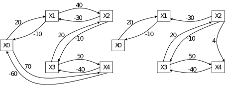
Figure 12: The distance graphs of the STPs of Appendices B (left) and C (Right). The edges $(X_{i},X_{j})$ whose weights are infinite and the loops $(X_{i},X_{i})$ are not shown.

We apply the bdArc-Consistency algorithm bdAC-3 to $P$. The initial binarized domains of the variables and the initialisation of the queue $Q$ are as follows:

1. $Q=\{(X_{1},X_{2}),(X_{2},X_{1}),(X_{2},X_{3}),(X_{3},X_{2}),(X_{3},X_{4}),$ $(X_{4},X_{3})\}$

2. $\begin{array}[]{l||l|l|l|l}X_{i}&X_{1}&X_{2}&X_{3}&X_{4}\\ \hline\cr bd(X_{i})&[10,20]&{\rm I\!R}&{\rm I\!R}&[60,70]\end{array}$

We take in turn the pairs in $Q$ for propagation. When a pair $(X_{i},X_{j})$, with $ij\not=0$, is taken from $Q$ for propagation, we apply the path-consistency operation on triangle $(X_{0},X_{j},X_{i})$: $P_{0i}=P_{0i}\cap P_{0j}\otimes P_{ji}$. If $P_{0i}$ is modified, the pairs $(X_{k},X_{i})$ such that $k\not=0$, $k\not=i$, $k\not=j$ and $P$ has a constraint on $X_{k}$ and $X_{i}$, that are no longer in $Q$, reenter the queue. bdAC-3 will terminate when a binarized domain becomes empty, indicating inconsistency of the initial STP, or the queue becomes empty, indicating that the STP has been made bdArc-Consistent.

Step 1: we take the pair $(X_{1},X_{2})$ from $Q$ and apply the path-consistency operation on triangle $(X_{0},X_{2},X_{1})$:

1. $P_{01}=P_{01}\cap P_{02}\otimes P_{21}=[10,20]\cap{\rm I\!R}\otimes[-40,-30]=[10,20]$

2. No modification, and the new configuration is:

3. $Q=\{(X_{2},X_{1}),(X_{2},X_{3}),(X_{3},X_{2}),(X_{3},X_{4}),(X_{4},X_{3})\}$

4. $\begin{array}[]{l||l|l|l|l}X_{i}&X_{1}&X_{2}&X_{3}&X_{4}\\ \hline\cr bd(X_{i})&[10,20]&{\rm I\!R}&{\rm I\!R}&[60,70]\end{array}$

Step 2: we take the pair $(X_{2},X_{1})$:

1. $P_{02}=P_{02}\cap P_{01}\otimes P_{12}={\rm I\!R}\cap[10,20]\otimes[30,40]=[40,60]$

2. There is modification, and the new configuration is:

3. $Q=\{(X_{2},X_{3}),(X_{3},X_{2}),(X_{3},X_{4}),(X_{4},X_{3})\}$

4. $\begin{array}[]{l||l|l|l|l}X_{i}&X_{1}&X_{2}&X_{3}&X_{4}\\ \hline\cr bd(X_{i})&[10,20]&[40,60]&{\rm I\!R}&[60,70]\end{array}$

Step 3: we take the pair $(X_{2},X_{3})$:

1. $P_{02}=P_{02}\cap P_{03}\otimes P_{32}=[40,60]\cap{\rm I\!R}\otimes[10,20]=[40,60]$

2. No modification, and the new configuration is:

3. $Q=\{(X_{3},X_{2}),(X_{3},X_{4}),(X_{4},X_{3})\}$

4. $\begin{array}[]{l||l|l|l|l}X_{i}&X_{1}&X_{2}&X_{3}&X_{4}\\ \hline\cr bd(X_{i})&[10,20]&[40,60]&{\rm I\!R}&[60,70]\end{array}$

Step 4: we take the pair $(X_{3},X_{2})$:

1. $P_{03}=P_{03}\cap P_{02}\otimes P_{23}={\rm I\!R}\cap[40,60]\otimes[-20,-10]=[20,50]$

2. There is modification, and the new configuration is:

3. $Q=\{(X_{3},X_{4}),(X_{4},X_{3})\}$

4. $\begin{array}[]{l||l|l|l|l}X_{i}&X_{1}&X_{2}&X_{3}&X_{4}\\ \hline\cr bd(X_{i})&[10,20]&[40,60]&[20,50]&[60,70]\end{array}$

Step 5: we take the pair $(X_{3},X_{4})$:

1. $P_{03}=P_{03}\cap P_{04}\otimes P_{43}=[20,50]\cap[60,70]\otimes[-50,-40]=[20,50]\cap[10,30]=[20,30]$

2. There is modification, and the new configuration is:

3. The pair $(X_{2},X_{3})$ reenters to $Q$, which becomes $Q=\{(X_{4},X_{3}),(X_{2},X_{3})\}$

4. $\begin{array}[]{l||l|l|l|l}X_{i}&X_{1}&X_{2}&X_{3}&X_{4}\\ \hline\cr bd(X_{i})&[10,20]&[40,60]&[20,30]&[60,70]\end{array}$

Step 6: we take the pair $(X_{4},X_{3})$:

1. $P_{04}=P_{04}\cap P_{03}\otimes P_{34}=[60,70]\cap[20,30]\otimes[40,50]=[60,70]\cap[60,80]=[60,70]$

2. No modification, and the new configuration is:

3. $Q=\{(X_{2},X_{3})\}$

4. $\begin{array}[]{l||l|l|l|l}X_{i}&X_{1}&X_{2}&X_{3}&X_{4}\\ \hline\cr bd(X_{i})&[10,20]&[40,60]&[20,30]&[60,70]\end{array}$

Step 7: we take the pair $(X_{2},X_{3})$:

1. $P_{02}=P_{02}\cap P_{03}\otimes P_{32}=[40,60]\cap[20,30]\otimes[10,20]=[40,60]\cap[30,50]=[40,50]$

2. There is modification, and the new configuration is:

3. The pair $(X_{1},X_{2})$ reenters to $Q$, which becomes $Q=\{(X_{1},X_{2})\}$

4. $\begin{array}[]{l||l|l|l|l}X_{i}&X_{1}&X_{2}&X_{3}&X_{4}\\ \hline\cr bd(X_{i})&[10,20]&[40,50]&[20,30]&[60,70]\end{array}$

Step 8: we take the pair $(X_{1},X_{2})$:

1. $P_{01}=P_{01}\cap P_{02}\otimes P_{21}=[10,20]\cap[40,60]\otimes[-40,-30]=[10,20]\cap[0,30]=[10,20]$

2. No modification, and the new configuration is:

3. $Q=\{\}$

4. $\begin{array}[]{l||l|l|l|l}X_{i}&X_{1}&X_{2}&X_{3}&X_{4}\\ \hline\cr bd(X_{i})&[10,20]&[40,50]&[20,30]&[60,70]\end{array}$

The queue $Q$ is empty, and no (binarized) domain has become empty. bdAC-3 terminates and the resulting STP is bdArc-Consistent. The minimal (binarized) domains of variables $X_{1},X_{2},X_{3},X_{4}$ are, respectively, $[10,20]$, $[40,50]$, $[20,30]$ and $[60,70]$. Therefore, if we consider the distance graph of the original STP, we have the following:

1. the distances of the shortest paths from $X_{0}$ to $X_{1},X_{2},X_{3},X_{4}$ are, respectively, $20$, $50$, $30$ and $70$

2. the distances of the shortest paths from each of $X_{1},X_{2},X_{3},X_{4}$ to $X_{0}$ are, respectively, $-10$, $-40$, $-20$ and $-60$.  

Appendix C bdAC-3 applied to an STP: illustration 2

In the STP of the example in Appendix B, we replace constraint $c_{3}$ with $(X_{2}-X_{1})\in[30,+\infty)$, remove constraint $c_{2}$, and add the constraint $(X_{4}-X_{2})\in(-\infty,4]$. We get the STP $P=(X,C)$, whose distance graph is given by Figure 12(Right):

1. $X=\{X_{0},X_{1},X_{2},X_{3},X_{4}\}$ and

2. $C=\{c_{1}:(X_{1}-X_{0})\in[10,20],c_{2}:(X_{2}-X_{1})\in[30,+\infty),c_{3}:(X_{3}-X_{2})\in[-20,-10],c_{4}:(X_{4}-X_{2})\in(-\infty,4],c_{5}:(X_{4}-X_{3})\in[40,50]\}$.

The rooted distance graph of $P$ does have a negative ciruit that is not reachable from $X_{0}$, but from which $X_{0}$ is reachable. The proposed algorithm, contrary to Bellman-Ford-Moore’s, will detect the negative circuit; this amounts to detecting the inconsistency of the STP.

We apply the bdArc-Consistency algorithm bdAC-3 to $P$. The initial binarized domains of the variables and the initialisation of the queue $Q$ are as follows:

1. $Q=\{(X_{1},X_{2}),(X_{2},X_{1}),(X_{2},X_{3}),(X_{3},X_{2}),(X_{2},X_{4}),$ $(X_{4},X_{2}),(X_{3},X_{4}),$ $(X_{4},X_{3})\}$

2. $\begin{array}[]{l||l|l|l|l}X_{i}&X_{1}&X_{2}&X_{3}&X_{4}\\ \hline\cr bd(X_{i})&[10,20]&{\rm I\!R}&{\rm I\!R}&{\rm I\!R}\end{array}$

We take in turn the pairs in $Q$ for propagation. When a pair $(X_{i},X_{j})$, with $ij\not=0$, is taken from $Q$ for propagation, we apply the path-consistency operation on triangle $(X_{0},X_{j},X_{i})$: $P_{0i}=P_{0i}\cap P_{0j}\otimes P_{ji}$. If $P_{0i}$ is modified, the pairs $(X_{k},X_{i})$ such that $k\not=0$, $k\not=i$, $k\not=j$ and $P$ has a constraint on $X_{k}$ and $X_{i}$, that were but are no longer in $Q$, reenter the queue. bdAC-3 will terminate when a binarized domain becomes empty, indicating inconsistency of the initial STP, or the queue becomes empty, indicating that the STP has been made bdArc-Consistent.

Step 1: we take the pair $(X_{2},X_{1})$:

1. $P_{02}=P_{02}\cap P_{01}\otimes P_{12}={\rm I\!R}\cap[10,20]\otimes[30,+\infty)=[40,+\infty)$

2. There is modification, and the new configuration is:

3. $Q=\{(X_{1},X_{2}),(X_{2},X_{3}),(X_{3},X_{2}),(X_{2},X_{4}),$ $(X_{4},X_{2}),(X_{3},X_{4}),$ $(X_{4},X_{3})\}$

4. $\begin{array}[]{l||l|l|l|l}X_{i}&X_{1}&X_{2}&X_{3}&X_{4}\\ \hline\cr bd(X_{i})&[10,20]&[40,+\infty)&{\rm I\!R}&{\rm I\!R}\end{array}$

Step 2: we take the pair $(X_{2},X_{3})$:

1. $P_{02}=P_{02}\cap P_{03}\otimes P_{32}=[40,+\infty)\cap{\rm I\!R}\otimes[10,20]=[40,+\infty)$

2. No modification, and the new configuration is:

3. $Q=\{(X_{1},X_{2}),(X_{3},X_{2}),(X_{2},X_{4}),$ $(X_{4},X_{2}),(X_{3},X_{4}),$ $(X_{4},X_{3})\}$

4. $\begin{array}[]{l||l|l|l|l}X_{i}&X_{1}&X_{2}&X_{3}&X_{4}\\ \hline\cr bd(X_{i})&[10,20]&[40,+\infty)&{\rm I\!R}&{\rm I\!R}\end{array}$

Step 3: we take the pair $(X_{3},X_{2})$:

1. $P_{03}=P_{03}\cap P_{02}\otimes P_{23}={\rm I\!R}\cap[40,+\infty)\otimes[-20,-10]=[20,+\infty)$

2. There is modification, and the new configuration is:

3. $Q=\{(X_{1},X_{2}),(X_{2},X_{4}),$ $(X_{4},X_{2}),(X_{3},X_{4}),$ $(X_{4},X_{3})\}$

4. $\begin{array}[]{l||l|l|l|l}X_{i}&X_{1}&X_{2}&X_{3}&X_{4}\\ \hline\cr bd(X_{i})&[10,20]&[40,+\infty)&[20,+\infty)&{\rm I\!R}\end{array}$

Step 4: we take the pair $(X_{2},X_{4})$:

1. $P_{02}=P_{02}\cap P_{04}\otimes P_{42}=[40,+\infty)\cap{\rm I\!R}\otimes[-4,+\infty)=[40,+\infty)$

2. No modification, and the new configuration is:

3. $Q=\{(X_{1},X_{2}),(X_{4},X_{2}),(X_{3},X_{4}),$ $(X_{4},X_{3})\}$

4. $\begin{array}[]{l||l|l|l|l}X_{i}&X_{1}&X_{2}&X_{3}&X_{4}\\ \hline\cr bd(X_{i})&[10,20]&[40,+\infty)&[20,+\infty)&{\rm I\!R}\end{array}$

Step 5: we take the pair $(X_{4},X_{2})$:

1. $P_{04}=P_{04}\cap P_{02}\otimes P_{24}={\rm I\!R}\cap[40,+\infty)\otimes(-\infty,4]={\rm I\!R}$

2. No modification, and the new configuration is:

3. $Q=\{(X_{1},X_{2}),(X_{3},X_{4}),$ $(X_{4},X_{3})\}$

4. $\begin{array}[]{l||l|l|l|l}X_{i}&X_{1}&X_{2}&X_{3}&X_{4}\\ \hline\cr bd(X_{i})&[10,20]&[40,+\infty)&[20,+\infty)&{\rm I\!R}\end{array}$

Step 6: we take the pair $(X_{3},X_{4})$:

1. $P_{03}=P_{03}\cap P_{04}\otimes P_{43}=[20,+\infty)\cap{\rm I\!R}\otimes[-50,-40]=[20,+\infty)$

2. No modification, and the new configuration is:

3. $Q=\{(X_{1},X_{2}),(X_{4},X_{3})\}$

4. $\begin{array}[]{l||l|l|l|l}X_{i}&X_{1}&X_{2}&X_{3}&X_{4}\\ \hline\cr bd(X_{i})&[10,20]&[40,+\infty)&[20,+\infty)&{\rm I\!R}\end{array}$

Step 7: we take the pair $(X_{4},X_{3})$:

1. $P_{04}=P_{04}\cap P_{03}\otimes P_{34}={\rm I\!R}\cap[20,+\infty)\otimes[40,50]=[60,+\infty)$

2. There is modification. $(X_{2},X_{4})$ reenters the queue, and the new configuration is:

3. $Q=\{(X_{1},X_{2}),(X_{2},X_{4})\}$

4. $\begin{array}[]{l||l|l|l|l}X_{i}&X_{1}&X_{2}&X_{3}&X_{4}\\ \hline\cr bd(X_{i})&[10,20]&[40,+\infty)&[20,+\infty)&[60,+\infty)\end{array}$

Step 8: we take the pair $(X_{2},X_{4})$:

1. $P_{02}=P_{02}\cap P_{04}\otimes P_{42}=[40,+\infty)\cap[60,+\infty)\otimes[-4,+\infty)=[56,+\infty)$

2. There is modification, and the new configuration is:

3. The pair $(X_{3},X_{2})$ reenters the queue $Q$, which becomes $Q=\{(X_{1},X_{2}),(X_{3},X_{2})\}$

4. $\begin{array}[]{l||l|l|l|l}X_{i}&X_{1}&X_{2}&X_{3}&X_{4}\\ \hline\cr bd(X_{i})&[10,20]&[56,+\infty)&[20,+\infty)&[60,+\infty)\end{array}$

Step 9: we take the pair $(X_{3},X_{2})$:

1. $P_{03}=P_{03}\cap P_{02}\otimes P_{23}=[20,+\infty)\cap[56,+\infty)\otimes[-20,-10]=[36,+\infty)$

2. There is modification, and the new configuration is:

3. The pair $(X_{4},X_{3})$ reenters the $Q$, which becomes $Q=\{(X_{1},X_{2}),(X_{4},X_{3})\}$

4. $\begin{array}[]{l||l|l|l|l}X_{i}&X_{1}&X_{2}&X_{3}&X_{4}\\ \hline\cr bd(X_{i})&[10,20]&[56,+\infty)&[36,+\infty)&[60,+\infty)\end{array}$

Step 10: we take the pair $(X_{4},X_{3})$:

1. $P_{04}=P_{04}\cap P_{03}\otimes P_{34}=[60,+\infty)\cap[36,+\infty)\otimes[40,50]=[76,+\infty)$

2. There is modification, and new configuration is:

3. The pair $(X_{2},X_{4})$ reenters the $Q$, which becomes $Q=\{(X_{1},X_{2}),(X_{2},X_{4})\}$

4. $\begin{array}[]{l||l|l|l|l}X_{i}&X_{1}&X_{2}&X_{3}&X_{4}\\ \hline\cr bd(X_{i})&[10,20]&[56,+\infty)&[36,+\infty)&[76,+\infty)\end{array}$

Step 11: we take the pair $(X_{2},X_{4})$:

1. $P_{02}=P_{02}\cap P_{04}\otimes P_{42}=[56,+\infty)\cap[76,+\infty)\otimes[-4,+\infty)=[72,+\infty)$

2. There is modification, and the new configuration is:

3. The pair $(X_{3},X_{2})$ reenters the queue $Q$, which becomes $Q=\{(X_{1},X_{2}),(X_{3},X_{2})\}$

4. $\begin{array}[]{l||l|l|l|l}X_{i}&X_{1}&X_{2}&X_{3}&X_{4}\\ \hline\cr bd(X_{i})&[10,20]&[72,+\infty)&[36,+\infty)&[76,+\infty)\end{array}$

Step 12: we take the pair $(X_{3},X_{2})$:

1. $P_{03}=P_{03}\cap P_{02}\otimes P_{23}=[36,+\infty)\cap[72,+\infty)\otimes[-20,-10]=[52,+\infty)$

2. There is modification, and the new configuration is:

3. The pair $(X_{4},X_{3})$ reenters the queue $Q$, which becomes $Q=\{(X_{1},X_{2}),(X_{4},X_{3})\}$

4. $\begin{array}[]{l||l|l|l|l}X_{i}&X_{1}&X_{2}&X_{3}&X_{4}\\ \hline\cr bd(X_{i})&[10,20]&[72,+\infty)&[52,+\infty)&[76,+\infty)\end{array}$

Step 13: we take the pair $(X_{4},X_{3})$:

1. $P_{04}=P_{04}\cap P_{03}\otimes P_{34}=[76,+\infty)\cap[52,+\infty)\otimes[40,50]=[92,+\infty)$

2. There is modification of $P_{04}$ with $-lowerB(P_{04})=-92$ strictly smaller than $\mbox{path-lb}(P)=-90$. The conditions of Theorem 3 get violated, and the situation corresponds to a detection of a negative circuit. The algorithm terminates with a negative answer to the consistency problem of $P$ (line 4 of the REVISE procedure of Figure 3).

References

- Aho et al. [1976] A V Aho, J E Hopcroft, and J D Ullman. The Design and Analysis of Computer Algorithms. Addison-Wesley Publishing Co., 1976.
- Allen [1983] James Allen. Maintaining knowledge about temporal intervals. Communications of the Association for Computing Machinery, 26(11):832–843, 1983.
- Belhadji and Isli [1998] S Belhadji and A Isli. Temporal constraint satisfaction techniques in job shop scheduling problem solving. Constraints, 3(2-3):203–211, 1998.
- Bellman [1958] R Bellman. On a routing problem. Quarterly of Applied Mathematics, 16(1):87–90, 1958.
- Bessière et al. [1996] C Bessière, A Isli, and G Ligozat. Global consistency in interval algebra networks: tractable subclasses. In W Wahlster, editor, Proceedings of the 12th European Conference on Artificial Intelligence (ECAI), pages 3–7, Budapest, 1996. John Wiley.
- Bessière [1996] C Bessière. A simple way to improve path consistency processing in interval algebra networks. In William J. Clancey and Daniel S. Weld, editors, Proceedings of the 13th American Conference on Artificial Intelligence (AAAI), pages 375–380. AAAI Press / The MIT Press, 1996.
- Broxvall et al. [2002] Mathias Broxvall, Peter Jonsson, and Jochen Renz. Disjunctions, independence, refinements. Artif. Intell., 140(1/2):153–173, 2002.
- Carlier et al. [1985] J Carlier, P Chrétienne, and C Girault. Modelling scheduling problems with timed petri nets. In G Rozenberg, H J Genrich, and G Roucairol, editors, Advances in Petri nets 1984, volume 188 of Lecture Notes in Computer Science, pages 62–84. Springer, 1985.
- Cervoni et al. [1994] R Cervoni, A Cesta, and A Oddi. Managing dynamic temporal constraint networks. In Proceedings of the Second International Conference on Artificial Intelligence Planning Systems (AIPS), pages 13–18. AAAI Press, 1994.
- Cesta and Oddi [1996] A Cesta and A Oddi. Gaining efficiency and flexibility in the simple temporal problem. In Proceedings of the Third International Workshop on Temporal Representation and Reasoning (TIME), pages 45–50. IEEE Computer Society, 1996.
- Davis [1989] E Davis. Private communication. 1989.
- Dechter et al. [1991] R Dechter, I Meiri, and J Pearl. Temporal constraint networks. Artificial Intelligence, 49:61–95, 1991.
- Dechter [1992] R Dechter. From local to global consistency. Artificial Intelligence, 55:87–107, 1992.
- Dincbas et al. [1990] M Dincbas, H Simonis, and P van Hentenryck. Solving large combinatorial problems in logic programming. Journal of Logic Programming, 8(1):75–93, 1990.
- Ford and Fulkerson [1962] L R Ford and D R Fulkerson. Flows in Networks. Princeton University Press, New Jersey, 1962.
- Freuder [1982] E C Freuder. A sufficient condition for backtrack-free search. Journal of the Association for Computing Machinery, 29:24–32, 1982.
- Isli [2001] A Isli. On deciding Consistency for CSPs of Cyclic Time Intervals. In I Russel and J F Kolen, editors, Proceedings of the Fourteenth International Florida Artificial Intelligence Research Society Conference (FLAIRS), pages 547–551, Key West, Florida, USA, May 21-23 2001. AAAI Press.
- Kautz and Ladkin [1991] H Kautz and P Ladkin. Integrating metric and qualitative temporal reasoning. In Proceedings of the 9th American Conference on Artificial Intelligence (AAAI), pages 241–246, Anaheim, CA, 1991. AAAI/MIT Press.
- Kong et al. [2018] S Kong, J H Lee, and S Li. Multiagent simple temporal problem: The arc-consistency approach. In Proceedings of the 32nd American Conference on Artificial Intelligence (AAAI), pages 6219–6226. AAAI Press, 2018.
- Ladkin and Maddux [1994] P Ladkin and R Maddux. On binary Constraint Problems. Journal of the Association for Computing Machinery, 41(3):435–469, 1994.
- Ladkin and Reinefeld [1992] P Ladkin and A Reinefeld. Effective solution for qualitative constraint problems. Artificial Intelligence, 57:105–124, 1992.
- Ligozat [1996] Gerard Ligozat. A new proof of tractability for ord-horn relations. In William J. Clancey and Daniel S. Weld, editors, Proceedings of the 13th American Conference on Artificial Intelligence (AAAI), pages 395–401. AAAI Press / The MIT Press, 1996.
- Mackworth [1977] A K Mackworth. Consistency in networks of relations. Artificial Intelligence, 8:99–118, 1977.
- Montanari [1974] U Montanari. Networks of constraints: fundamental properties and applications to picture processing. Information Sciences, 7:95–132, 1974.
- Moore [1959] E F Moore. The shortest path through a maze. In Proceedings of an International Symposium on the Theory of Switching (Cambridge, Massachusetts, 2–5 April 1957), page 285–292, Cambridge, 1959. Harvard University Press.
- Nebel and Bürckert [1995] Bernhard Nebel and Hans-Jürgen Bürckert. Reasoning about temporal relations: A maximal tractable subclass of allen’s interval algebra. J. ACM, 42(1):43–66, 1995.
- Nebel [1997] Bernhard Nebel. Solving hard qualitative temporal reasoning problems: Evaluating the efficiency of using the ord-horn class. Constraints An Int. J., 1(3):175–190, 1997.
- Papadimitriou and Steiglitz [1982] C H Papadimitriou and K Steiglitz. Combinatorial Optimisation: Algorithms and Complexity. 1982.
- Planken et al. [2008] L Planken, M de Weerdt, and R van der Krogt. P3C: A new algorithm for the simple temporal problem. In Proceedings of the 18th International Conference on Automated Planning and Scheduling ICAPS, pages 256–263. AAAI Press, 2008.
- Pratt [1977] V R Pratt. Two easy theories whose combination is hard. Technical report, Massachusetts Institute of Technology, 1977.
- Sadeh et al. [1995] N Sadeh, K Sycara, and Y Xiong. Backtracking techniques for the job shop scheduling constraint satisfaction problem. Artificial Intelligence, 76:455–480, 1995.
- Schwalb and Dechter [1997] E Schwalb and R Dechter. Processing disjunctions in temporal constraint networks. Artificial Intelligence, 193:29–61, 1997.
- Shostak [1981] R E Shostak. Deciding linear inequalities by computing loop residues. J. ACM, 28(4):769–779, 1981.
- Stergiou and Koubarakis [2000] K Stergiou and M Koubarakis. Backtracking algorithms for disjunctions of temporal constraints. Artificial Intelligence, 120(1):81–117, 2000.
- van Beek and Manchak [1996] Peter van Beek and Dennis W. Manchak. The design and experimental analysis of algorithms for temporal reasoning. J. Artif. Intell. Res., 4:1–18, 1996.
- van Beek [1992] Peter van Beek. Reasoning about qualitative temporal information. Artificial Intelligence, 58(1-3):297–326, 1992.