Equitable Allocations of Indivisible Chores

Abstract

We study fair allocation of indivisible chores (i.e., items with non-positive value) among agents with additive valuations. An allocation is deemed fair if it is (approximately) equitable, which means that the disutilities of the agents are (approximately) equal. Our main theoretical contribution is to show that there always exists an allocation that is simultaneously equitable up to one chore (EQ1) and Pareto optimal (PO), and to provide a pseudopolynomial-time algorithm for computing such an allocation. In addition, we observe that the Leximin solution—which is known to satisfy a strong form of approximate equitability in the goods setting—fails to satisfy even EQ1 for chores. It does, however, satisfy a novel fairness notion that we call equitability up to any duplicated chore. Our experiments on synthetic as well as real-world data obtained from the Spliddit website reveal that the algorithms considered in our work satisfy approximate fairness and efficiency properties significantly more often than the algorithm currently deployed on Spliddit.

1 Introduction

Imagine a group of agents who must collectively complete a set of undesirable or costly tasks, also known as chores. For example, household chores such as cooking, cleaning, and maintenance need to be distributed among the members of the household. As another example, consider the allocation of global climate change responsibilities among the member nations in a treaty (Traxler, 2002). These responsibilities could entail producing more clean energy, reducing overall emissions, research and development, etc. In both of these cases, it is important that the allocation of chores is fair and that it takes advantage of heterogeneity in agents’ preferences. For instance, someone might prefer to cook than to clean, while someone else might have the opposite preference. Likewise, different countries might have competitive advantages in different areas.

Problems of this nature can be modeled mathematically as chore division problems, first introduced by Gardner (1978). Each agent incurs a non-positive utility, or cost (in terms of money, time, or general dissatisfaction), from completing each chore that she reports to a central mechanism. In this paper, our focus is on designing mechanisms to divide the chores among the agents equitably. An allocation of chores is equitable if all agents get exactly the same (dis)utility from their allocated chores. Other fairness properties can, of course, be considered too—for instance, envy-freeness dictates that no agent should prefer another agent’s assigned chores to her own. While this is not the main focus of our work, we do consider (approximate) envy-freeness in conjunction with (approximate) equitability.

Equitable allocations have been studied extensively in the context of allocating goods (i.e., items with non-negative value). When the goods are divisible (or, even more generally, in the cake-cutting setting), perfectly equitable allocations are guaranteed to exist (Dubins and Spanier, 1961; Alon, 1987). For indivisible goods, though, perfect equitability might not be possible, but approximate versions can still be achieved (Gourvès et al., 2014; Freeman et al., 2019).

At first glance, the problem of chore division appears similar to the goods division problem. However, there are subtle technical differences between the two settings. In the context of (approximate) envy-freeness, this contrast has been noted in several works (Peterson and Su, 2009; Bogomolnaia et al., 2018, 2017; Brânzei and Sandomirskiy, 2019). To take one example, it is known that an allocation of goods that is both envy-free up to one good and Pareto optimal can be found by allocating goods so that the product of the agents’ utilities—the Nash social welfare—is maximized (Caragiannis et al., 2019). However, maximizing the product of utilities is not sensible when valuations are negative, and no analogous procedure is known for the case of chores.

		EQ1	EQX	DEQ1	DEQX
Without PO	Existence	Always exists	Always exists	Always exists	Always exists
		(3)	(3)	(5)	(5)
	Computation	Poly time	Poly time	Poly time	?
		(3)	(3)	(6)
With PO	Existence	Always exists	Might not exist	Always exists	Always exists
		(Theorem 2)	(1)	(5)	(5)
	Computation	Pseudopoly time	Strongly NP-hard	?	?
		(Theorem 2)	(Theorem 1)

Table 1: Summary of our theoretical results. Each cell contains the existence/computation results for various combinations of fairness and efficiency properties. Open questions are marked with ‘?’.

In this paper, we demonstrate a similar set of differences between the goods and chores settings in the context of equitability. Our focus is on equitability up to one/any chore (EQ1/EQX) which requires that pairwise violations of equitability can be eliminated by removing some/any chore from the bundle of the less happy agent.

For goods division, Freeman et al. (2019) showed that equitability up to any good and Pareto optimality are achieved simultaneously by the Leximin algorithm. However, we show that in the chores setting, Leximin does not even guarantee equitability up to one chore (EQ1) (2). Further, while we are able to give an algorithm that outputs an EQ1 and PO allocation in pseudopolynomial time (Theorem 2), modifying a similar algorithm of Freeman et al. (2019), we show that an allocation satisfying EQX and PO may not exist, in contrast to the goods setting (1).

The fact that EQX+PO could fail to exist and that the Leximin allocation may not be EQ1 leads us to consider other relaxations of perfect equitability. To this end, we define the equitability up to one/any duplicated chore (DEQ1/DEQX) properties. These properties require that pairwise equitability can be restored by duplicating a chore from the less happy agent’s bundle and adding it to the more happy agent’s bundle, rather than removing a chore from the less happy agent’s bundle. Interestingly, we find that the “duplicate” relaxations are satisfied by the Leximin allocation (5), restoring a formal justification for that algorithm even in the chores setting. Table 1 summarizes our results.

Finally, we complement our theoretical results with extensive simulations on both simulated data and data gathered from the popular fair division website Spliddit  (Goldman and Procaccia, 2015). We find that on a large fraction of instances ($>80\%$), Leximin satisfies all of the approximate properties that we consider, in addition to Pareto optimality. We therefore consider it to be the best choice for use in practice, matching the observation of Freeman et al. (2019) in the case of goods. When the runtime of the Leximin algorithm is prohibitive (computing the Leximin allocation is NP-hard), our simulations reveal that our pseudopolynomial algorithm for achieving EQ1 and PO is a reasonable choice for achieving these as well as other properties on a large fraction of instances.

1.1 Related Work

Fair division of indivisible chores has received considerable interest in recent years. Aziz et al. (2017), Huang and Lu (2019), Aziz et al. (2019b), and Aziz et al. (2019c) study approximation algorithms for max-min fair share (MMS) allocation of chores. Brânzei and Sandomirskiy (2019) show that an allocation that is envy-free up to the removal of two chores (${\textrm{{EF}}}^{1}_{1}$) and Pareto optimal (PO) always exists and can be computed in polynomial time if the number of agents is fixed. Segal-Halevi (2018b) has studied competitive equilibria in the allocation of indivisible chores with unequal budgets.

Several papers study a model with mixed items, wherein an item can be a good for one agent and a chore for another. Bogomolnaia et al. (2017) examine this model for divisible items and show that unlike the goods-only case, the set of competitive utility profiles (Varian, 1974; Eisenberg and Gale, 1959) can be multivalued; for the chores-only problem, the multiplicity can be exponential in the number of agents/items (Bogomolnaia et al., 2018). Segal-Halevi (2018a) and Meunier and Zerbib (2019) consider a generalization of the cake-cutting problem to the mixed utilities setting, and study envy-free divisions with connected pieces. Aziz et al. (2019a) study indivisible mixed items and provide a polynomial-time algorithm for computing EF1 allocations even for non-additive valuations. For the same model, Aziz et al. (2019d) provide a polynomial-time algorithm for computing allocations that are Pareto optimal (PO) and proportional up to one item (Prop1). Sandomirskiy and Segal-Halevi (2019) consider envy-free/proportional and Pareto optimal divisions that minimize the number of fractionally assigned items. Notably, none of this work examines equitability for indivisible items.

Equitability for indivisible chores has been studied by Bouveret et al. (2019) in a model where the items constitute the vertices of a graph, and each agent should be assigned a connected subgraph. This work does not consider Pareto optimality, and the space of permissible allocations in this model is different from ours, making the two sets of results incomparable. Caragiannis et al. (2012) study the worst-case welfare loss due to equitability (i.e., ‘price of equitability’) for indivisible chores, but do not consider approximate fairness.

For goods, equitability as a fairness notion has been studied extensively, mostly in the context of cake-cutting (Dubins and Spanier, 1961; Brams et al., 2006; Cechlárová and Pillárová, 2012; Brams et al., 2012; Cechlárová et al., 2013; Brams et al., 2013; Aumann and Dombb, 2015; Procaccia and Wang, 2017; Chèze, 2017). Our work bears most similarity to the work of Gourvès et al. (2014) and Freeman et al. (2019), who define the notions of EQX and EQ1, respectively.

2 Preliminaries

Problem instance

An instance $\langle[n],[m],\mathcal{V}\rangle$ of the fair division problem is defined by a set of $n\in{\mathbb{N}}$ agents $[n]=\{1,2,\dots,n\}$, a set of $m\in{\mathbb{N}}$ chores $[m]=\{1,2,\dots,m\}$, and a valuation profile $\mathcal{V}=\{v_{1},v_{2},\dots,v_{n}\}$ that specifies the preferences of every agent $i\in[n]$ over each subset of the chores in $[m]$ via a valuation function $v_{i}:2^{[m]}\rightarrow\mathbb{Z}_{\leq 0}$. Note that we assume that the valuations are non-positive integers; most of our results hold without this assumption but Theorem 2 requires it.

We will also assume that the valuation functions are additive, i.e., for any agent $i\in[n]$ and any set of chores $S\subseteq[m]$, $v_{i}(S)\coloneqq\sum_{j\in S}v_{i}(\{j\})$, where $v_{i}(\emptyset)=0$. For a singleton chore $j\in[m]$, we will write $v_{i,j}$ instead of $v_{i}(\{j\})$. The valuation functions are said to be normalized if for all agents $i,j\in[n]$, we have $v_{i}([m])=v_{j}([m])$. We will assume throughout, without loss of generality, that for each chore $j\in[m]$, there exists some agent $i\in[n]$ with a non-zero valuation for it (i.e., $v_{i,j}<0$), and for each agent $i\in[n]$, there exists a chore $j\in[m]$ that it has non-zero value for.

Allocation

An allocation $A\coloneqq(A_{1},\dots,A_{n})$ is an $n$-partition of the set of chores $[m]$, where $A_{i}\subseteq[m]$ is the bundle allocated to the agent $i$ (note that $A_{i}$ can be empty). Given an allocation $A$, the utility of agent $i\in[n]$ for the bundle $A_{i}$ is $v_{i}(A_{i})=\sum_{j\in A_{i}}v_{i,j}$.

Equitability

An allocation $A$ is said to be (a) equitable (EQ) if for every pair of agents $i,k\in[n]$, we have $v_{i}(A_{i})=v_{k}(A_{k})$; (b) equitable up to one chore (EQ1) if for every pair of agents $i,k\in[n]$ such that $A_{i}\neq\emptyset$, there exists a chore $j\in A_{i}$ such that $v_{i}(A_{i}\setminus\{j\})\geq v_{k}(A_{k})$, and (c) equitable up to any chore (EQX) if for every pair of agents $i,k\in[n]$ such that $A_{i}\neq\emptyset$ and for every chore $j\in A_{i}$ such that $v_{i,j}<0$, we have $v_{i}(A_{i}\setminus\{j\})\geq v_{k}(A_{k})$. These notions have been previously studied for goods by Gourvès et al. (2014) and Freeman et al. (2019). Our presentation of the notions of (approximate) equitability for chores—in particular, the idea of removing a chore from the less-happy agent’s bundle—follows the formulation used by Aziz et al. (2019a) and Aleksandrov (2018) in defining the analogous relaxations of envy-freeness (see below).

Envy-freeness

An allocation $A$ is said to be (a) envy-free (EF) if for every pair of agents $i,k\in[n]$, we have $v_{i}(A_{i})\geq v_{i}(A_{k})$; (b) envy-free up to one chore (EF1) if for every pair of agents $i,k\in[n]$ such that $A_{i}\neq\emptyset$, there exists a chore $j\in A_{i}$ such that $v_{i}(A_{i}\setminus\{j\})\geq v_{i}(A_{k})$, and (c) envy-free up to any chore (EFX) if for every pair of agents $i,k\in[n]$ such that $A_{i}\neq\emptyset$ and for every chore $j\in A_{i}$ such that $v_{i,j}<0$, we have $v_{i}(A_{i}\setminus\{j\})\geq v_{i}(A_{k})$. The notions of EF, EF1, and EFX were proposed in the context of goods allocation by Foley (1967), Budish (2011), and Caragiannis et al. (2019), respectively.

It is easy to see that envy-freeness and equitability (and their corresponding relaxations) become equivalent when the valuations are identical, i.e., for every $j\in[m]$, $v_{i,j}=v_{k,j}$ for all $i,k\in[n]$.

Proposition 1.

When agents have identical valuations, an allocation satisfies EF/EFX/EF1 if and only if it satisfies EQ/EQX/EQ1.

Pareto optimality

An allocation $A$ is Pareto dominated by allocation $B$ if $v_{k}(B_{k})\geq v_{k}(A_{k})$ for every agent $k\in[n]$ with at least one of the inequalities being strict. A Pareto optimal (PO) allocation is one that is not Pareto dominated by any other allocation.

Leximin-optimal allocation

A Leximin-optimal (or simply Leximin) allocation of chores is one that maximizes the minimum utility that any agent achieves, subject to which the second minimum utility is maximized, and so on. The utilities induced by a Leximin allocation are unique, although there may exist more than one such allocation (Dubins and Spanier, 1961).

3 Theoretical Results

This section presents our theoretical contributions. We will first consider equitability and its relaxations (Section 3.1), followed by combining these notions with Pareto optimality (Section 3.2), and subsequently also considering envy-freeness (Section 3.3). Finally, we will discuss a novel approximation of equitability called equitability up to a duplicated chore (Section 3.4).

3.1 Equitability and its Relaxations

As discussed previously, an equitable (EQ) allocation is not guaranteed to exist when allocating indivisible chores. In addition, the computational problem of determining whether a given instance has an equitable allocation turns out to be NP-complete even for identical valuations (2). The proof uses a standard reduction from 3-Partition and is therefore omitted.

Proposition 2.

Determining whether a given fair division instance admits an equitable $(\textrm{{EQ}})$ allocation is strongly NP-complete even for identical valuations.

The negative results regarding the existence and computation of exact equitability are in complete contrast with those of its relaxations. Indeed, when allocating indivisible chores, there always exists an allocation that is equitable up to any chore (EQX). Furthermore, such an allocation can be computed in polynomial time via a simple greedy procedure (3). This algorithm is a straightforward adaptation of the algorithm of Gourvès et al. (2014) for computing EQX allocations of goods.

Proposition 3.

An EQX allocation of chores always exists and can be computed in polynomial time.

Proof.

(Sketch) Our algorithm iteratively assigns the chores to the agents according to the following assignment rule: At each step, the happiest agent (i.e., one whose utility is closest to zero) is asked to select a chore from the set of available chores that it dislikes the most (i.e., the chore that gives it the most negative utility).

It is easy to see that the chore assigned most recently to any agent is also its favorite (or least disliked) chore in its bundle. Thus, if an allocation is EQX before assigning a chore, then it continues to be EQX after it. The claim now follows by induction, since an empty allocation is EQX to begin with. ∎

The positive result in 3 offers an interesting comparison between envy-freeness and equitability: It is not known whether an EFX allocation is even guaranteed to exist for chores, but an EQX allocation can always be computed in polynomial time.

3.2 Equitability and Pareto Optimality

We will now consider equitability together with Pareto optimality. From 2, it is easy to see that checking the existence of an equitable and Pareto optimal (EQ+PO) allocation is strongly NP-hard (since every allocation is Pareto optimal under identical valuations). Therefore, we will strive for achieving Pareto optimality alongside approximate equitability, specifically EQ1 and EQX.

We will start by considering equitability up to any chore (EQX) and Pareto optimality. For goods allocation, Freeman et al. (2019) have shown that equitability up to any good and Pareto optimality can be simultaneously achieved using the Leximin allocation. By contrast, as we show in 1, there might not exist an allocation that is equitable up to any chore and Pareto optimal, even when there are only two agents.

Example 1 (Non-existence of EQX+PO).

Consider an instance with three chores $c_{1},c_{2},c_{3}$ and two agents $a_{1},a_{2}$ with strictly negative (and normalized) valuations as shown below:

	$c_{1}$	$c_{2}$	$c_{3}$
$a_{1}$	$-2$	$-50$	$-50$
$a_{2}$	$-97$	$-4$	$-1$

Of the eight possible allocations in the above instance, the two allocations that assign all chores to a single agent, namely $A^{1}\coloneqq(\{c_{1},c_{2},c_{3}\},\{\emptyset\})$ and $A^{2}\coloneqq(\{\emptyset\},\{c_{1},c_{2},c_{3}\})$ violate EQX and can be immediately ruled out. Any other allocation must assign exactly one chore to one agent and two to the other.

Of the three allocations in which $a_{1}$ is assigned exactly one chore, namely $A^{3}\coloneqq(\{c_{1}\},\{c_{2},c_{3}\})$, $A^{4}\coloneqq(\{c_{2}\},\{c_{1},c_{3}\})$, and $A^{5}\coloneqq(\{c_{3}\},\{c_{1},c_{2}\})$, none satisfies EQX. Therefore, these allocations can be ruled out as well.

This leaves us with the three allocations in which $a_{2}$ is assigned exactly one chore, namely $A^{6}\coloneqq(\{c_{1},c_{2}\},\{c_{3}\})$, $A^{7}\coloneqq(\{c_{2},c_{3}\},\{c_{1}\})$, and $A^{8}\coloneqq(\{c_{1},c_{3}\},\{c_{2}\})$. Among these, only $A^{7}$ satisfies EQX. However, $A^{7}$ is Pareto dominated by the allocation $A^{3}$; indeed, $v_{1}(A^{7})=-100<v_{1}(A^{3})=-2$ and $v_{2}(A^{7})=-97<v_{2}(A^{3})=-5$. Therefore, the above instance does not admit an EQX+PO allocation. ∎

To make matters worse, determining whether a given instance admits an EQX and PO allocation turns out to be strongly NP-hard.

Theorem 1 (Strong NP-hardness of EQX+PO).

Determining whether a given fair division instance admits an allocation that is simultaneously equitable up to any chore $(\textrm{{EQX}}{})$ and Pareto optimal $(\textrm{{PO}}{})$ is strongly NP-hard, even for strictly negative and normalized valuations.

Proof.

We will show a reduction from 3-Partition, which is known to be strongly NP-hard (Garey and Johnson, 1979, Theorem 4.4). An instance of 3-Partition consists of a set $X=\{b_{1},\dots,b_{3r}\}$ of $3r$ positive integers where $r\in{\mathbb{N}}$, and the goal is to find a partition of $X$ into $r$ subsets $X^{1},\dots,X^{r}$ such that the sum of numbers in each subset is equal to $B\coloneqq\frac{1}{r}\sum_{b_{i}\in X}b_{i}$. We will assume, without loss of generality, that for every $i\in[3r]$, $b_{i}$ is even and $b_{i}\geq 2$. As a result, we can also assume, without loss of generality, that $B$ is even.

We will construct a fair division instance with $r+1$ agents and $4r+2$ chores (see Table 2). The set of agents consists of $r$ main agents $a_{1},\dots,a_{r}$ and a dummy agent $d$. The set of chores consists of $3r$ main chores $C_{1},\dots,C_{3r}$, $r$ signature chores $S_{1},\dots,S_{r}$, and two dummy chores $D_{1},D_{2}$. The valuations of the agents are specified as follows: For every $i\in[r]$ and $j\in[3r]$, agent $a_{i}$ values the main chore $C_{j}$ at $-b_{j}$, the signature chore $S_{i}$ at $-1$, and all other chores at a large negative number $-L$, where $-L<-rB-1$. The dummy agent $d$ values the dummy chores $D_{1}$ and $D_{2}$ at $-1$ and $-B$, respectively, and all other chores at a large negative number $-L^{\prime}$. In the interest of having normalized valuations, we can set $L^{\prime}\coloneqq\frac{(r-1)B+(r+1)L}{4r}$. It is easy to show using standard calculus that $-L^{\prime}<-B$ for all $r\geq 3$. Since the condition $r\geq 3$ holds without loss of generality, we will assume throughout that $-L^{\prime}<-B$.

	$C_{1}$	…	$C_{3r}$	$S_{1}$	$S_{2}$	…	$S_{r}$	$D_{1}$	$D_{2}$
$a_{1}$	$-b_{1}$	…	$-b_{3r}$	$-1$	$-L$	…	$-L$	$-L$	$-L$
$a_{2}$	$-b_{1}$	…	$-b_{3r}$	$-L$	$-1$	…	$-L$	$-L$	$-L$
⋮		⋮			⋮			⋮
$a_{r}$	$-b_{1}$	…	$-b_{3r}$	$-L$	$-L$	…	$-1$	$-L$	$-L$
$d$	$-L^{\prime}$	…	$-L^{\prime}$	$-L^{\prime}$	$-L^{\prime}$	…	$-L^{\prime}$	$-1$	$-B$

Table 2: Chores instance used in the proof of Theorem 1.

We will now argue the equivalence of solutions.

$(\Rightarrow)$ Let $X^{1},\dots,X^{r}$ be a solution of 3-Partition. Then, the desired allocation $A$ can be constructed as follows: For every $i\in[r]$, the main agent $a_{i}$ gets the signature chore $S_{i}$ as well as the chores corresponding to the numbers in $X^{i}$. The dummy agent gets the two dummy chores. The allocation $A$ is Pareto optimal because each chore is assigned to an agent that has the highest valuation for it (thus, $A$ maximizes social welfare). Also, each agent’s valuation in $A$ is $-B-1$, implying that $A$ is equitable, and hence also EQX.

$(\Leftarrow)$ Now suppose that there exists an EQX and Pareto optimal allocation $A$. Below, we will make a series of observations about $A$ that will help us infer a solution of 3-Partition using $A$.

Claim 1.

No agent gets an empty bundle in $A$.

Proof.

(of Claim 1) If an agent gets an empty bundle, then some other agent will get four or more chores (as more than $4r$ chores will need to be allocated among $r$ other agents). Since all valuations are strictly negative, this results in a violation of EQX. ∎

Claim 2.

Each main agent $a_{i}$ gets its signature chore $S_{i}$ in $A$.

Proof.

(of Claim 2) From Claim 1, we know that $a_{i}$ owns at least one chore in $A$. Fix any chore $j\in A_{i}$. Suppose $S_{i}$ is assigned to an agent $k$ in $A$. Notice that the valuation of agent $k$ for $S_{i}$ is either $-L$ or $-L^{\prime}$ (depending of whether $k$ is a main or a dummy agent). This is also the smallest valuation that agent $k$ has for any chore (recall that $-L<-rB-1$ and $-L^{\prime}<-B$). Furthermore, since $-b_{i}\leq-2$ for every $i\in[3r]$, $S_{i}$ is the unique favorite chore of agent $a_{i}$. Therefore, after exchanging the chores $j$ and $S_{i}$, the valuation of agent $k$ cannot decrease (due to additivity), and the valuation of agent $a_{i}$ necessarily increases. Thus, the new allocation is a Pareto improvement over $A$, which is a contradiction. ∎

Claim 3.

The chore $D_{1}$ is assigned to the dummy agent $d$ in $A$.

Proof.

(of Claim 3) By an argument similar to that in the proof of Claim 2, we can show that if $D_{1}$ is not assigned to $d$, then a Pareto improving swap between $d$ and the owner of $D_{1}$ is possible. ∎

Claim 4.

The chore $D_{2}$ is assigned to the dummy agent $d$ in $A$.

Proof.

(of Claim 4) Suppose, for contradiction, that $D_{2}$ is assigned to main agent $a_{i}$ in $A$. From Claim 2, we know that $a_{i}$ is also assigned its signature chore $S_{i}$. Since $S_{i}$ is the favorite chore of $a_{i}$, the EQX condition requires that for every other main agent $a_{k}$,

$$v_{k}(A_{k})\leq v_{i}(A_{i}\setminus\{S_{i}\})\leq v_{i}(\{D_{2}\})=-L.$$

Even if $a_{k}$ is assigned all the remaining chores whose assignment has not been finalized yet (this includes the $3r$ main chores), its valuation will still only be $-rB-1>-L$. This would imply a violation of EQX condition between $a_{i}$ and $a_{k}$, which is a contradiction. ∎

From Claims 3 and 4, we know that $D_{1},D_{2}\in A_{d}$. Therefore, by EQX condition, the following must hold for every main agent $a_{i}$:

$$v_{i}(A_{i})\leq v_{d}(A_{d}\setminus\{D_{1}\})\leq v_{d}(\{D_{2}\})=-B.$$

From Claim 2, we know that $a_{i}$ gets its signature chore $S_{i}$. Thus, the valuation of $a_{i}$ for the remaining items in its bundle must be

$$v_{i}(A_{i}\setminus\{S_{i}\})\leq-B+1.$$ (1)

Since the assignment of all signature and dummy chores has been fixed, the set $A_{i}\setminus\{S_{i}\}$ can only have main chores. By assumption, main agents have even-valued valuations for main chores. By additivity of valuations, the quantity $v_{i}(A_{i}\setminus\{S_{i}\})$ must also be even. Also, $-B$ is even, so $-B+1$ must be odd, and therefore the inequality in Equation 1 must be strict. Thus, $v_{i}(A_{i}\setminus\{S_{i}\})\leq-B$.

We can now infer a solution of 3-Partition as follows: For every $i\in[r]$, the set $X^{i}$ contains those numbers whose corresponding chores are included in $A_{i}\setminus\{S_{i}\}$. Since $v_{i}(A_{i}\setminus\{S_{i}\})\leq-B$, it follows that all main chores must be assigned among the main agents, implying that $X^{1},\dots,X^{r}$ constitute a valid partition of $X$. Furthermore, the sum of numbers in the set $X^{i}$ cannot exceed $B$, or otherwise the sum of numbers in some other set $X^{k}$ will be strictly less than $B$, which would violate the above inequality. Hence, $X^{1},\dots,X^{r}$ is a valid solution of 3-Partition, as desired. ∎

The negative results concerning the existence and computation of EQX+PO lead us to consider a weaker relaxation of equitability, namely equitability up to one chore (EQ1). A natural starting point in studying the existence of EQ1+PO allocations is the Leximin solution, as it yields strong positive results for the goods setting (Freeman et al., 2019). Unfortunately, as 2 shows, Leximin sometimes fails to satisfy EQ1 (as well as EF1) for chores.

Example 2 (Leximin fails EQ1 and EF1).

Consider the following instance with four chores and three agents with normalized and strictly negative valuations:

	$c_{1}$	$c_{2}$	$c_{3}$	$c_{4}$
$a_{1}$	$-1$	$-5$	$-5$	$-5$
$a_{2}$	$-1$	$-2$	$-2$	$-11$
$a_{3}$	$-6$	$-5$	$-3$	$-2$

We will show that the allocation $A$ given by $A_{1}=\{c_{1}\}$, $A_{2}=\{c_{2},c_{3}\}$, and $A_{3}=\{c_{4}\}$ is Leximin-optimal. Suppose, for contradiction, that another allocation $B$ is a Leximin improvement over $A$. The utility profile induced by $A$ is $(-1,-4,-2)$, and therefore, for any chore $j$ and agent $i$ such that $j\in B_{i}$, we must have that $v_{i,j}\geq-4$.

The chore $c_{4}$ is valued at less than $-4$ by both $a_{1}$ and $a_{2}$, so we must have $c_{4}\in B_{3}$. Similarly, we can fix $c_{2}\in B_{2}$. This, in turn, forces us to fix $c_{3}\in B_{2}$, since otherwise if $c_{3}\in B_{3}$, then the utility of $a_{3}$ will be $-5<-4$, which would violate the Leximin improvement assumption. By a similar argument, we have $c_{1}\in B_{1}$. This, however, implies that $A$ and $B$ are identical, which is a contradiction. Therefore, $A$ must be Leximin. Notice that $A$ violates EQ1 and EF1 for the pair $(a_{1},a_{2})$. ∎

Another natural approach to show the existence of EQ1+PO allocations could be to use the relax-and-round framework. Specifically, one could start from an egalitarian-equivalent solution (Pazner and Schmeidler, 1978) (i.e., a fractional allocation that is perfectly equitable and minimizes the agents’ disutilities), and use a rounding algorithm to achieve EQ1. However, there is a simple example where this approach fails.

The failure of Leximin and the relax-and-round framework in achieving EQ1 prompts us to consider a different approach for studying approximately fair and Pareto optimal allocations. This approach, which is based on Fisher markets (Brainard and Scarf, 2000), has been successfully used in the goods model to provide an algorithmic framework for computing EF1+PO (Barman et al., 2018) and EQ1+PO (Freeman et al., 2019) allocations. Note that the existence of such allocations was established by means of computationally intractable methods, namely the Maximum Nash Welfare and Leximin solutions (Caragiannis et al., 2019; Freeman et al., 2019).

Briefly, the idea is to start with an allocation that is an equilibrium of some Fisher market. By the first welfare theorem (Mas-Colell et al., 1995), such an allocation is guaranteed to be Pareto optimal. By using a combination of local search and price change steps, our algorithm converges to an approximately equitable equilibrium, which gives an approximately equitable and Pareto optimal allocation. An important distinguishing feature of our algorithm is that while the existing Fisher market based approaches use price-rise (Barman et al., 2018; Freeman et al., 2019), our algorithm instead uses price-drop as the natural option for negative valuations.

Our main result in this section (Theorem 2) establishes the existence of EQ1 and PO allocations using the markets framework.

Theorem 2 (Algorithm for EQ1+PO).

Given any chores instance with additive and integral valuations, an allocation that is equitable up to one chore $(\textrm{{EQ{1}}})$ and Pareto optimal $(\textrm{{PO}}{})$ always exists and can be computed in ${\mathcal{O}}(\textrm{{poly}}(m,n,|v_{\min}|))$ time, where $v_{\min}=\min_{i,j}v_{i,j}$.

In particular, when the valuations are polynomially bounded (i.e., for every $i\in[n]$ and $j\in[m]$, $v_{i,j}\leq\textrm{{poly}}(m,n)$), our algorithm computes an EQ1 and PO allocation in polynomial time. Whether an EQ1+PO allocation can be computed in polynomial time without this assumption is an interesting avenue for future research.

The proof of Theorem 2 is deferred to Section 6.1. Here, we will provide an informal overview of the algorithm by demonstrating its execution on the instance in 2 where Leximin fails to satisfy EQ1.

(a)

(b)

(c)

(d)

Figure 1: Executing the EQ1+PO algorithm from Theorem 2 on the instance in 2. The solid (respectively, dashed) edges denote items that are allocated to (respectively, in the MBB set of) an agent. The edge labels denote the valuations, and the numbers next to the agent and chore nodes denote the utilities and the prices, respectively.

Example 3.

Consider once again the instance in 2. Our algorithm in Theorem 2 works in three phases. In Phase 1, the algorithm creates an equilibrium allocation by assigning each chore to an agent that has the highest valuation for it and setting its price to be (the absolute value of) the owner’s valuation; see Figure 1a. This ensures that the allocation satisfies the maximum bang-per-buck or MBB property (i.e., each agent’s bundle consists only of items with the highest valuation-to-price ratio for that agent). The MBB property guarantees that the allocation at hand is an equilibrium of some Fisher market, and therefore Pareto optimal.

The allocation constructed in Phase 1 is not EQ1 as $a_{2}$ gets three negatively valued chores and $a_{1}$ gets none. So, the algorithm switches to Phase 2, where it uses local search to address the equitability violations. Specifically, if there is an EQ1 violation, then there must be one involving the ‘happiest’ agent, i.e., agent with the highest utility (shaded in green in Figure 1a). The algorithm now proceeds to transferring the chores, one at a time, from unhappy agents to the happiest agent while ensuring that all exchanges take place in an MBB-consistent manner. In our example, the chore $c_{1}$, which is already in the MBB set of agent $a_{1}$, is transferred from $a_{2}$ to $a_{1}$ (see Figure 1b).

Despite the aforementioned exchange, the allocation is still not EQ1 as $\{a_{1},a_{2}\}$ once again constitute a violating pair. Furthermore, the happiest agent is already assigned its unique MBB chore, so no additional MBB-consistent transfers are possible. Thus, the algorithm switches to Phase 3.

In Phase 3, the algorithm creates new MBB edges in the agent-item graph by changing the prices. Specifically, the price of chore $c_{1}$ is lowered until one or more of the remaining chores enter the MBB set of agent $a_{1}$. Indeed, once the price of $c_{1}$ is lowered from $\$1$ to $\$0.4$, all other chores become MBB for agent $a_{1}$ (see Figure 1c). As soon as the opportunity for MBB-consistent exchange becomes available, the algorithm switches back to Phase 2 to perform an exchange. This time, chore $c_{2}$ is transferred from $a_{2}$ to $a_{1}$ (see Figure 1d). The new allocation is EQ1, so the algorithm terminates and returns the current allocation as output. ∎

Remark 1.

We already know from 1 that EQX+PO is a strictly more demanding property combination than EQ1+PO in terms of existence. That is, an EQX+PO allocation might fail to exist even though an EQ1+PO allocation is guaranteed to exist (Theorem 2). Our results in Theorems 1 and 2 show a similar separation between the two notions in terms of computation: Although an EQ1+PO allocation can be computed in pseudopolynomial-time (Theorem 2), there cannot be a pseudopolynomial-time algorithm for checking the existence of EQX+PO allocations unless P=NP.

3.3 Equitability, Pareto Optimality, and Envy-Freeness

We will now consider all three notions—equitability, envy-freeness, and Pareto optimality—together. It turns out that the existence result for EQ1+PO allocations does not hold up when we also require EF1 (4).

Proposition 4 (Non-existence of EQ1+EF1+PO).

There exists an instance with normalized and strictly negative valuations in which no allocation is simultaneously equitable up to one chore $(\textrm{{EQ{1}}})$, envy-free up to one chore $(\textrm{{EF{1}}})$, and Pareto optimal $(\textrm{{PO}}{})$.

Proof.

Consider the following instance with eight chores and four agents with normalized and strictly negative valuations:

	$c_{1}$	$c_{2}$	$c_{3}$	$c_{4}$	$c_{5}$	$c_{6}$	$c_{7}$	$c_{8}$
$a_{1}$	$-10$	$-10$	$-10$	$-10$	$-10$	$-10$	$-10$	$-10$
$a_{2}$	$-10$	$-10$	$-10$	$-10$	$-10$	$-10$	$-10$	$-10$
$a_{3}$	$-73$	$-1$	$-1$	$-1$	$-1$	$-1$	$-1$	$-1$
$a_{4}$	$-73$	$-1$	$-1$	$-1$	$-1$	$-1$	$-1$	$-1$

Suppose, for contradiction, that there exists an allocation $A$ that is EQ1, EF1, and PO. Then, we claim that $a_{1}$ gets exactly one chore in $A$. Indeed, $a_{1}$ cannot get three or more chores in $A$, since that would result in some other agent getting at most one chore, creating an EF1 violation with respect to $a_{1}$. If $a_{1}$ gets exactly two chores, then either $a_{3}$ or $a_{4}$ will create an EQ1 violation with respect to $a_{1}$. This is because one of $a_{3}$ and $a_{4}$ will necessarily miss out on $c_{1}$ and therefore have a utility of at least $-7$ from the remaining chores. Finally, if $a_{1}$ does not get any chore, then one of the other agents will get at least three chores. Because of strictly negative valuations, this will create an EQ1 violation with $a_{1}$. Therefore, $a_{1}$ gets exactly one chore in $A$. By a similar argument, so does $a_{2}$.

Therefore, a total of six chores are assigned between $a_{3}$ and $a_{4}$. Assume, without loss of generality, that $a_{3}$ gets at least three chores. Then, whoever of $a_{1}$ or $a_{2}$ misses out on $c_{1}$ will create an EF1 violation with respect to $a_{3}$, giving us the desired contradiction. ∎

Turning to the computational question, we notice that the allocation constructed in the proof of Theorem 1 is envy-free. Therefore, checking the existence of an EQX+PO+EF/EFX/EF1 allocation is also strongly NP-hard. We note that the analogous problem in the goods setting is also known to be computationally hard (Freeman et al., 2019).

Corollary 1 (Hardness of EQX+PO+EF/EFX/EF1).

Determining whether a given fair division instance admits an allocation that is simultaneously $X+Y+\textrm{{PO}}{}$, where $X$ refers to equitable up to any chore $(\textrm{{EQX}}{})$, and $Y$ refers to either envy-free $(\textrm{{EF}})$, envy-free up to any chore $(\textrm{{EFX}}{})$, or envy-free up to one chore $(\textrm{{EF{1}}})$, is strongly NP-hard, even for normalized valuations.

3.4 Equitability up to a Duplicated Chore

In this section, we will explore a slightly different version of approximate equitability for chores wherein instead of removing a chore from the less-happy agent’s bundle, we imagine adding a chore to the happier agent’s bundle. In particular, we will ask that pairwise jealousy should be removed by duplicating a single chore from the less happy agent’s bundle and adding it to the happier agent’s bundle.

Formally, an allocation $A$ is equitable up to one duplicated chore (DEQ1) if for every pair of agents $i,k\in[n]$ such that $A_{i}\neq\emptyset$, there exists a chore $j\in A_{i}$ such that $v_{i}(A_{i})\geq v_{k}(A_{k}\cup\{j\})$. An allocation $A$ is equitable up to any duplicated chore (DEQX) if for every pair of agents $i,k\in[n]$ such that $A_{i}\neq\emptyset$ and for every chore $j\in A_{i}$ such that $v_{i,j}<0$, we have $v_{i}(A_{i})\geq v_{k}(A_{k}\cup\{j\})$.

Proposition 5 (Existence of DEQX+PO).

Given any fair division instance with additive valuations, an allocation that is equitable up to any duplicated chore $(\textrm{{DEQX}}{})$ and Pareto optimal $(\textrm{{PO}}{})$ always exists.

Proof.

(Sketch) We will show that any Leximin-optimal allocation, say $A$, satisfies DEQX (Pareto optimality is easy to verify). Suppose, for contradiction, that there exist agents $i,k\in[n]$ with $A_{i}\neq\emptyset$ and some chore $j\in A_{i}$ such that $v_{i,j}<0$ and $v_{i}(A_{i})<v_{k}(A_{k}\cup\{j\})$. Let $B$ be an allocation derived from $A$ by transferring the chore $j$ from agent $i$ to agent $k$. That is, $B_{i}\coloneqq A_{i}\setminus\{j\}$, $B_{k}\coloneqq A_{k}\cup\{j\}$ and $B_{h}\coloneqq A_{h}$ for all $h\in[n]\setminus\{i,k\}$. Since DEQX is violated with respect to chore $j$, we have that $v_{i,j}<0$, and therefore $v_{i}(B_{i})=v_{i}(A_{i})-v_{i,j}>v_{i}(A_{i})$. Furthermore, $v_{k}(B_{k})=v_{k}(A_{k}\cup\{j\})>v_{i}(A_{i})$ by the DEQX violation condition. The utility of any other agent is unchanged. Therefore, $B$ is a ‘Leximin improvement’ over $A$, which is a contradiction. ∎

Thus, 5 shows that the duplicate version of approximate equitability (DEQX) compares favorably against the standard version (EQX) in the sense that a DEQX+PO allocation is guaranteed to exist whereas an EQX+PO allocation might not exist even with two agents and strictly negative valuations (1).

On the computational side, we find that a DEQ1 allocation of chores can be computed in polynomial time via a greedy algorithm.

Proposition 6.

A DEQ1 allocation of chores always exists and can be computed in polynomial time.

Proof.

Consider any fixed ordering $j_{1},j_{2},\dots,j_{m}$ of the chores. Our algorithm assigns the chore $j_{t}$ in the $t^{\text{th}}$ round. Let $A^{t-1}$ denote the (partial) allocation at the end of $t-1$ rounds. The algorithm assigns the chore $j_{t}$ to the agent $i_{t}$ defined as follows:

$$\textstyle i_{t}\in\arg\max_{i\in[n]}v_{i}(A^{t-1}_{i}\cup\{j_{t}\}).$$

That is, in a thought experiment where each agent gets a copy of the chore $j_{t}$, agent $i_{t}$ has the highest utility in the derived allocation. It is easy to see that the algorithm runs in polynomial time.

We will now use induction to show that the algorithm maintains a DEQ1 (partial) allocation at every step. This is certainly true prior to the first round, since an empty allocation is DEQ1. Suppose the partial allocations at the end of each of the first $t-1$ rounds, namely $A^{1},\dots,A^{t-1}$, satisfy DEQ1. We will argue that the same is true for the (partial) allocation $A^{t}$ at the end of the $t^{\text{th}}$ round.

Suppose, for contradiction, that $A^{t}$ fails DEQ1. That is, there exists a pair of agents $i,k\in[n]$ with $A^{t}_{i}\neq\emptyset$ such that $v_{i}(A^{t}_{i})<v_{k}(A^{t}_{k}\cup\{j\})$ for every chore $j\in A^{t}_{i}$. Then, the chore $j_{t}$ must have been assigned to agent $i$, i.e., $j_{t}\in A^{t}_{i}$. Indeed, if $j_{t}$ were to be assigned to any agent in $[n]\setminus\{i,k\}$, then the DEQ1 violation between $i$ and $k$ would have existed during round $t-1$, contradicting the fact that $A^{t-1}$ satisfies DEQ1. Furthermore, if $j_{t}$ were to be assigned to agent $k$, then agent $k$’s utility in round $t-1$ would have strictly exceeded its utility in round $t$, implying once again that DEQ1 violation between $i$ and $k$ would have existed in round $t-1$, which is a contradiction. Therefore, the chore $j_{t}$ must have been assigned to agent $i$ in round $t$.

We can now instantiate the DEQ1 violation condition for the chore $j_{t}$ to get $v_{i}(A^{t}_{i})<v_{k}(A^{t}_{k}\cup\{j_{t}\})$. Note that since $j_{t}$ is assigned to agent $i$, the bundle of agent $k$ remains unchanged between rounds $t-1$ and $t$, and therefore $A^{t}_{k}=A^{t-1}_{k}$ and $A^{t}_{i}=A^{t-1}_{i}\cup\{j_{t}\}$. Therefore, the DEQ1 violation can be rewritten as $v_{i}(A^{t-1}_{i}\cup\{j_{t}\})<v_{k}(A^{t-1}_{k}\cup\{j_{t}\})$. This implies that $i$ is not the highest utility agent in the thought experiment where each agent is assigned a (hypothetical) copy of the chore $j_{t}$, which is a contradiction. Therefore, the allocation $A^{t}$ must satisfy DEQ1. By induction, the same holds for the allocation returned by the algorithm. ∎

Unfortunately, the greedy algorithm in 6 does not guarantee a DEQX allocation. This stands in contrast to the situation for EQX, which is easily achieved by a greedy procedure. Settling the complexity of computing DEQX allocations is an interesting question for future work.

The complexity of computing an allocation that satisfies either DEQ1+PO or the stronger DEQX+PO also remains open. For DEQ1+PO, a natural approach would be to apply the market techniques used in Theorem 2, but that would require care as DEQ1 lacks the following “monotonicity” property that EQ1 has: If an allocation is not EQ1, then without loss of generality, there exists a violation with respect to the happiest agent. The same is not true for violations of DEQ1, which makes the analysis less obvious.

In Section 6.6, we explore a variant of DEQX, denoted as $\textrm{{DEQX}}^{0}$, in which the $v_{i,j}<0$ condition is not imposed on the duplicated chore $j$. With this modification, we show that computing an allocation satisfying $\textrm{{DEQX}}^{0}$+PO is NP-hard, as well as an equivalent result for the analogous notion of $\textrm{{EQX}}^{0}$.

Remark 2 (A tractable special case: binary valuations).

An instance is said to have binary valuations if for every agent $i\in[n]$ and every chore $j\in[m]$, we have $v_{i,j}\in\{-1,0\}$. For this restricted setting, there is a simple polynomial-time algorithm that gives an EQX+DEQX+EFX+PO allocation, as follows: If a chore is valued at $0$ by one or more agents, then it is arbitrarily assigned to an agent that values it at $0$. The remaining chores, which are valued at $-1$ by every agent, are assigned in a round-robin fashion.

4 Experiments

In this section, we will compare various algorithms in terms of how frequently they satisfy different combinations of fairness and efficiency properties on synthetic as well as real-world datasets.

For synthetic data, we follow the setup of Freeman et al. (2019) for goods by fixing $n=5$ agents, $m=20$ chores, and generating $1000$ instances with (the negation of) the valuations drawn from Dirichlet distribution. Additional pre-processing is required to ensure that the valuations are integral and normalized (see Section 6.7). Recall that integral valuations are required for Theorem 2. None of our results require normalization, but it is a natural condition to impose in practice.

The real-world dataset consists of $2613$ instances obtained from the Spliddit website (Goldman and Procaccia, 2015), with the number of agents ranging from $2$ to $15$, and the number of distinct chores ranging from $3$ to $1100$. Unlike the goods case, the “task division” segment of Spliddit allows distinct items to have multiple copies. Furthermore, instead of directly eliciting additive valuations (as is the case for goods), the website asks the users to specify their preferences in the form of multipliers; that is, given two chores $c_{1}$ and $c_{2}$, how many times would a user be willing to complete $c_{1}$ instead of completing $c_{2}$ once. As a result, the elicited valuations might not be integral. These design features force us to make a number of pre-processing decisions (see Section 6.7). In particular, in order to ensure integrality of valuations and remain as faithful as possible to the Spliddit instances, we have to give up on normalization.

We consider the following four algorithms: (1) The greedy algorithm from 3, (2) the Leximin solution, (3) the market-based algorithm Alg-eq1+po from Theorem 2, and (4) an algorithm currently deployed on the Spliddit website for dividing chores. The latter is a randomized algorithm that computes an ex ante equitable lottery over integral allocations (refer to Section 6.7 for details).

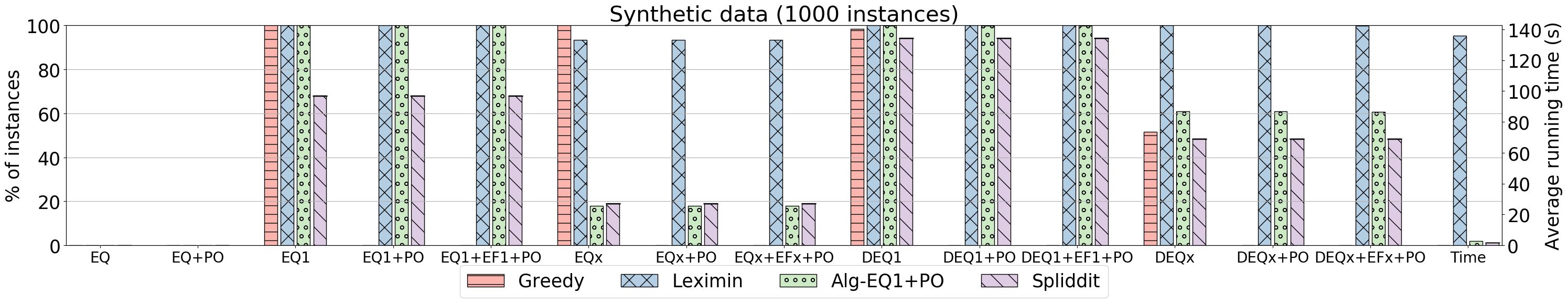
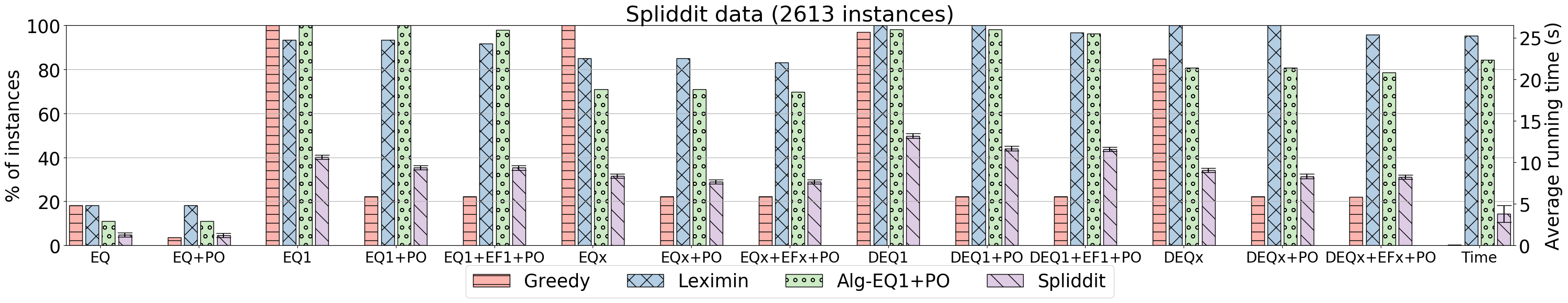
Figure 2: Experimental results for Synthetic (top) and Spliddit (bottom) datasets.

Figure 2 presents our experimental results. For each property combination (X-axis), the plots show the $\%$ of instances (Y-axis) for which each algorithm achieves those properties. The rightmost set of bars present a comparison of the running times. For the Spliddit algorithm, we plot the average values obtained from 100 runs, and the error bars show one standard deviation around the mean.

Starting with exact equitability, we observe that a very small fraction of instances ($<20\%$ in Spliddit and none in Synthetic) admit EQ and EQ+PO allocations, as one might expect. For the approximate notions, the greedy algorithm finds EQX allocations on all instances as advertised (3), but its performance drops off sharply when PO is also required; in particular, for Synthetic data, the greedy outcome is always Pareto dominated.

Leximin performs remarkably well across the board. In addition to satisfying DEQX+PO on all instances (5), it also satisfies EQX and EFX on more than $80\%$ of the instances in both datasets. Unfortunately, it is also the slowest of all algorithms, with an average runtime of $\sim$$140$ seconds on Synthetic dataset, compared to $<$$1$ second runtime of the fastest (greedy) algorithm.

The market-based algorithm Alg-eq1+po computes EQ1+PO allocations as expected (Theorem 2), and somewhat surprisingly, also satisfies DEQ1 (and EF1). However, its performance drops off when stronger approximations of EQX/DEQX are required.

The Spliddit algorithm is consistently (and often, significantly) outperformed by Leximin and Alg-eq1+po, even on the Spliddit dataset. The reason is that the Spliddit algorithm is perfectly equitable ex ante but not necessarily EQ1 ex post. As a result, it is better suited for ensuring fairness over time, say, when the same set of chores are repeatedly divided among the same agents, as noted on the Spliddit website.

In summary, Leximin emerges as the algorithm of choice in terms of simultaneously achieving approximate fairness and economic efficiency. We find it intriguing that the same algorithm was also a clear winner in the experimental analysis of Freeman et al. (2019) for goods, even though it is no longer provably EQX (or even EQ1). Equally intriguing is the fact that a currently deployed algorithm is outperformed by well-known (Leximin) and proposed (Alg-eq1+po) algorithms, thereby justifying the usefulness of analyzing (approximate) fairness for chore division.

5 Discussion

We studied equitable allocations of indivisible chores in conjunction with other well-known notions of fairness (envy-freeness) and economic efficiency (Pareto optimality), and provided a number of existential and computational results. Our results reveal some interesting points of difference between the goods and chores settings. While a modification of the market approach used by Freeman et al. (2019) to achieve EQ1+PO in the goods setting works for chores, it may be the case that no allocation satisfying EQX+PO exists in the chores setting. In response to this possible nonexistence, we have defined two new notions of relaxed equitability, DEQ1 and DEQX, that address equitability violations by adding chores to bundles rather than removing them. A number of open questions remain regarding the computation of allocations that satisfy these notions (with or without Pareto optimality). It may also be an interesting topic for future work to consider similar relaxations of envy-freeness in the chores setting.

In our experimental analysis, we have considered four different algorithms for chore division on both a real-world dataset gathered from the Spliddit website as well as a synthetic dataset. Our experiments present a compelling case that, in practice, Leximin is the best known algorithm for one-shot allocation of indivisible chores. This is true not only with respect to (relaxed) equitability, but also (relaxed) envy-freeness and Pareto optimality.

6 Appendix

6.1 Proof of Theorem 2

Recall the statement of Theorem 2.

See 2

Remark 3.

Given an instance $\mathcal{I}$ and a chore $j\in[m]$, let $S_{j}\coloneqq\{i\in[n]:v_{i,j}=0\}$ denote the set of agents that value $j$ at $0$. Then, in any Pareto optimal allocation, $j$ must be assigned to one of the agents in $S_{j}$. The choice of which agent in $S_{j}$ gets $j$ is immaterial from the viewpoint of EQ1. (Specifically, if $A$ is an EQ1+PO allocation that assigns chore $j$ to some agent $i\in S_{j}$, then an allocation derived from $A$ in which chore $j$ is assigned to some other agent $k\in S_{j}$ is also EQ1+PO.) Therefore, in our discussion on EQ1+PO allocations, we will only focus on strictly negative valuations.

The proof of Theorem 2 relies on the algorithm Alg-eq1+po (presented in Algorithm 1), and spans Sections 6.1, 6.2, 6.3, 6.4 and 6.5. We will start with some necessary definitions that will help us state Theorem 3, of which Theorem 2 is a special case.

Fractional allocations

A fractional allocation ${\mathrm{x}}\in[0,1]^{n\times m}$ refers to a fractional assignment of the chores to the agents such that exactly one unit of any chore is allocated, i.e., for every chore $j\in[m]$, $\sum_{i\in[n]}x_{i,j}=1$. We will use the term allocation to refer to an integral (or discrete) allocation and explicitly write fractional allocation otherwise.

${\varepsilon}$-Pareto optimality

Given any ${\varepsilon}\geq 0$, $A$ is ${\varepsilon}$-Pareto optimal (${\varepsilon}$-PO) if there does not exist an allocation $B$ such that $v_{k}(B_{k})\geq\frac{1}{(1+{\varepsilon})}v_{k}(A_{k})$ for every agent $k\in[n]$ with one of the inequalities being strict.

Fractional Pareto optimality

An allocation is fractionally Pareto optimal (fPO) if it not Pareto dominated by any fractional allocation. Thus, a fractionally Pareto optimal allocation is also Pareto optimal, but the converse is not necessarily true.

${\varepsilon}$-EQ1 allocation

Given any ${\varepsilon}\geq 0$, an allocation $A$ is ${\varepsilon}$-equitable up to one chore (${\varepsilon}$-EQ1) if for every pair of agents $i,k\in[n]$ such that $A_{i}\neq\emptyset$, there exists a chore $j\in A_{i}$ such that $\frac{1}{(1+{\varepsilon})}v_{i}(A_{i}\setminus\{j\})\geq v_{k}(A_{k})$.

Theorem 3.

Given any fair division instance with additive and strictly negative valuations and any ${\varepsilon}>0$, an allocation that is $3{\varepsilon}$-equitable up to one chore $(3{\varepsilon}\text{-}\textrm{{EQ{1}}})$ and ${\varepsilon}$-Pareto optimal $({\varepsilon}\text{-}\textrm{{PO}}{})$ always exists and can be computed in ${\mathcal{O}}(\textrm{{poly}}(m,n,\ln|v_{\min}|,\nicefrac{{1}}{{{\varepsilon}}}))$ time, where $v_{\min}=\min_{i,j}v_{i,j}$.

When $0<{\varepsilon}\leq\frac{1}{6m|v_{\min}|^{3}}$, we recover Theorem 2 as a special case of Theorem 3 (see Lemmas 16 and 18).

The remainder of this section develops the necessary preliminaries that will enable us to present our algorithm (Algorithm 1) and the analysis of its running time (Lemma 1) and correctness (Lemma 2). The detailed proofs of these results are presented subsequently in Sections 6.2, 6.3, 6.4 and 6.5.

Market Preliminaries

Fisher market for chores

A Fisher market for chores is an economic model that consists of a set of divisible chores and a set of agents (or buyers), each of whom is given a budget (or endowment) of virtual money (Brainard and Scarf, 2000). The agents are required to exhaust their budgets (of virtual money) to purchase a utility-maximizing subset of the chores but do not derive any utility from the money itself. Formally, a Fisher market is given by a tuple ${\mathcal{M}}=\langle[n],[m],\mathcal{V},e\rangle$ consisting of a set of $n$ agents $[n]=\{1,2,\dots,n\}$, a set of $m$ divisible chores $[m]=\{1,2,\dots,m\}$, a valuation profile $\mathcal{V}=\{v_{1},v_{2},\dots,v_{n}\}$ and a vector of endowments or budgets $\mathbf{e}=(e_{1},e_{2},\dots,e_{n})$.

A market outcome refers to a pair $(A,\mathbf{p})$, where $A=(A_{1},\dots,A_{n})$ is a fractional allocation of the $m$ chores, and $\mathbf{p}=(p_{1},\dots,p_{m})$ is a price vector that associates a non-negative price $p_{j}\geq 0$ with every chore $j\in[m]$. The spending of agent $i$ under the market outcome $(A,\mathbf{p})$ is given by $s_{i}=\sum_{j=1}^{m}A_{i,j}p_{j}$. The utility derived by the agent $i$ under $(A,\mathbf{p})$ depends linearly on the valuations as $v_{i}(A_{i})=\sum_{j=1}^{m}A_{i,j}v_{i,j}$.

MBB ratio and MBB set

Given a price vector $\mathbf{p}=(p_{1},\dots,p_{m})$, define the bang-per-buck ratio of agent $i$ for chore $j$ as $\alpha_{i,j}\coloneqq v_{i,j}/p_{j}$. The maximum bang-per-buck ratio (or MBB ratio) of agent $i$ is $\alpha_{i}\coloneqq\max_{j}\alpha_{i,j}$. The maximum bang-per-buck set (or MBB set) of agent $i$ is the set of all chores that maximize the bang-per-buck ratio for agent $i$ at the price vector $\mathbf{p}$, i.e., $\textrm{{MBB}}_{i}\coloneqq\{j\in[m]:v_{i,j}/p_{j}=\alpha_{i}\}$. Note that the MBB ratios are non-positive.

A market outcome $(A,\mathbf{p})$ constitutes an equilibrium if it satisfies the following conditions:

• Market clearing: Each chore is either priced at zero or is completely allocated. That is, for every chore $j\in[m]$, either $p_{j}=0$ or $\sum_{i=1}^{n}A_{i,j}=1$.

• Budget exhaustion: Agents spend their budgets completely, i.e., $s_{i}=e_{i}$ for all $i\in[n]$.

• MBB consistency: Each agent’s allocation is a subset of its MBB set. That is, for every agent $i\in[n]$ and every chore $j\in[m]$, $A_{i,j}>0\implies j\in\textrm{{MBB}}_{i}$. Note that MBB consistency implies that every agent maximizes its utility at the given prices $\mathbf{p}$ under the budget constraints.

7 presents the well-known first welfare theorem for Fisher markets (Mas-Colell et al., 1995, Chapter 16). For completeness, we provide a proof of this result for the chores setting.

Proposition 7 (First welfare theorem).

For a Fisher market with linear utilities, any equilibrium outcome is fractionally Pareto optimal $(\textrm{{fPO}}{})$.

Proof.

Suppose, for contradiction, that there exists an allocation $A$ and a price vector $\mathbf{p}$ such that $(A,\mathbf{p})$ is an equilibrium but $A$ is not fPO. Thus, there exists a fractional allocation, say ${\mathrm{x}}$, such that $v_{i}({\mathrm{x}}_{i})\geq v_{i}(A_{i})$ for all $i\in[n]$ and $v_{k}({\mathrm{x}}_{k})>v_{k}(A_{k})$ for some $k\in[n]$. Since both ${\mathrm{x}}$ and $A$ are required to assign all chores, we have that $\cup_{i\in[n]}{\mathrm{x}}_{i}=\cup_{i\in[n]}A_{i}=[m]$.

By MBB-consistency, we have that $v_{i}(A_{i})=p(A_{i})\cdot\alpha_{i}$ for every $i\in[n]$, where $\alpha_{i}$ is the MBB ratio for agent $i$, and $p(A_{i})\coloneqq\sum_{j\in A_{i}}p_{j}$ is the price of the bundle $A_{i}$. Since ${\mathrm{x}}$ is not guaranteed to satisfy MBB-consistency, we have that $v_{i}({\mathrm{x}}_{i})\leq p({\mathrm{x}}_{i})\cdot\alpha_{i}$ for every $i\in[n]$. Substituting these relations in the aforementioned inequalities, we get that $p({\mathrm{x}}_{i})\cdot\alpha_{i}\geq p(A_{i})\cdot\alpha_{i}$ for all $i\in[n]$ and $p({\mathrm{x}}_{k})\cdot\alpha_{k}>p(A_{k})\cdot\alpha_{k}$ for some $k\in[n]$.

Recall from Section 2 that for each chore, there exists some agent with a non-zero valuation for it, and for each agent, there exists a chore that it has non-zero value for. This implies that $\alpha_{i}<0$ for every agent $i\in[n]$. Thus, $p({\mathrm{x}}_{i})\leq p(A_{i})$ for all $i\in[n]$ and $p({\mathrm{x}}_{k})<p(A_{k})$ for some $k\in[n]$. By summing these inequalities for all agents, we get that $p([m])=\sum_{i\in[n]}p({\mathrm{x}}_{i})<\sum_{i\in[n]}p(A_{i})=p([m])$, which is a contradiction. Hence, $A$ must be fPO. ∎

MBB-Allocation graph and alternating paths

Given a Fisher market ${\mathcal{M}}=\langle[n],[m],\mathcal{V},e\rangle$, let $A$ and $\mathbf{p}$ denote an integral allocation and a price vector for ${\mathcal{M}}$ respectively. An MBB-allocation graph is an undirected bipartite graph $G$ with vertex set $[n]\cup[m]$ and an edge between agent $i\in[n]$ and chore $j\in[m]$ if either $j\in A_{i}$ (called an allocation edge) or $j\in\textrm{{MBB}}_{i}$ (called an MBB edge). Notice that if $A$ is MBB-consistent (i.e., $j\in A_{i}\implies j\in\textrm{{MBB}}_{i}$), then the allocation edges are a subset of MBB edges.

For an MBB-allocation graph, define an alternating path $P=(i,j_{1},i_{1},j_{2},i_{2},\dots,i_{\ell-1},j_{\ell},k)$ from agent $i$ to agent $k$ (and involving the agents $i_{1},i_{2},\dots,i_{\ell-1}$ and the chores $j_{1},j_{2},\dots,j_{\ell}$) as a series of alternating MBB and allocation edges such that $j_{1}\in\textrm{{MBB}}_{i}\cap A_{i_{1}}$, $j_{2}\in\textrm{{MBB}}_{i_{1}}\cap A_{i_{2}}$,$\dots$, $j_{\ell}\in\textrm{{MBB}}_{i_{\ell-1}}\cap A_{k}$. If such a path exists, we say that agent $k$ is reachable from agent $i$ via an alternating path. In this case, the length of path $P$ is $2\ell$ since it consists of $\ell$ allocation edges and $\ell$ MBB edges.

Reachability set

Let $G$ denote the MBB-allocation graph of a Fisher market for the outcome $(A,\mathbf{p})$. Fix a source agent $i\in[n]$ in $G$. Define the level of an agent $k\in[n]$ as half the length of the shortest alternating path from $i$ to $k$ if one exists (i.e., if $k$ is reachable from $i$), otherwise set the level of $k$ to be $n$. The level of the source agent $i$ is defined to be $0$. The reachability set $\mathcal{R}_{i}$ of agent $i$ is defined as a level-wise collection of all agents that are reachable from $i$, i.e., $\mathcal{R}_{i}=(\mathcal{R}_{i}^{0},\mathcal{R}_{i}^{1},\mathcal{R}_{i}^{2},\dots,)$, where $\mathcal{R}_{i}^{\ell}$ denotes the set of agents that are at level $\ell$ with respect to agent $i$. Note that given an MBB-allocation graph, a reachability set can be constructed in polynomial time via breadth-first search.

Given a reachability set $\mathcal{R}_{i}$, we can redefine an alternating path as a set of alternating MBB and allocation edges connecting agents at a lower level to those at a higher level. Formally, we will call a path $P=(i,j_{1},i_{1},j_{2},i_{2},\dots,i_{\ell-1},j_{\ell},k)$ alternating if (1) $j_{1}\in\textrm{{MBB}}_{i}\cap A_{i_{1}}$, $j_{2}\in\textrm{{MBB}}_{i_{1}}\cap A_{i_{2}}$,$\dots$, $j_{\ell}\in\textrm{{MBB}}_{i_{\ell-1}}\cap A_{k}$, and (2) ${\mathrm{level}}(i)<{\mathrm{level}}(i_{1})<{\mathrm{level}}(i_{2})<\dots<{\mathrm{level}}(i_{\ell-1})<{\mathrm{level}}(k)$. Thus, an alternating path cannot have edges between agents at the same level.

Violators and path-violators

Given a Fisher market ${\mathcal{M}}$ and an allocation $A$, an agent $i\in[n]$ with the highest valuation among all the agents is called the reference agent, i.e., $i\in\arg\max_{k\in[n]}v_{k}(A_{k})$. An agent $k\in[n]$ is said to be a violator if for every chore $j\in A_{k}$, we have that $v_{k}(A_{k}\setminus\{j\})<v_{i}(A_{i})$, where $i$ is the reference agent. Notice that the allocation $A$ is EQ1 if and only if there is no violator.

Given any ${\varepsilon}>0$, an agent $k\in[n]$ is an ${\varepsilon}$-violator if for every chore $j\in A_{k}$, we have $\frac{1}{(1+{\varepsilon})}v_{k}(A_{k}\setminus\{j\})<v_{i}(A_{i})$. Thus, an agent can be a violator without being an ${\varepsilon}$-violator. An allocation $A$ is ${\varepsilon}$-EQ1 if and only if there is no ${\varepsilon}$-violator.

A closely related notion is that of a path-violator. Let $i$ and $\mathcal{R}_{i}$ denote the reference agent and its reachability set respectively. An agent $k\in\mathcal{R}_{i}$ is a path-violator with respect to the alternating path $P=(i,j_{1},i_{1},j_{2},i_{2},\dots,i_{\ell-1},j_{\ell},k)$ if $v_{k}(A_{k}\setminus\{j_{\ell}\})<v_{i}(A_{i})$. Note that a path-violator (along a path $P$) need not be a violator as there might exist some chore $j\in A_{k}$ not on the path $P$ such that $v_{k}(A_{k}\setminus\{j\})\geq v_{i}(A_{i})$. Finally, given any ${\varepsilon}>0$, an agent $k\in\mathcal{R}_{i}$ is an ${\varepsilon}$-path-violator with respect to the alternating path $P=(i,j_{1},i_{1},\dots,j_{\ell},k)$ if $\frac{1}{(1+{\varepsilon})}v_{k}(A_{k}\setminus\{j_{\ell}\})<v_{i}(A_{i})$.

${\varepsilon}$-rounded instance

Given any ${\varepsilon}>0$, an ${\varepsilon}$-rounded instance refers to a fair division instance $\langle[n],[m],\mathcal{V}\rangle$ in which the valuations are either zero or the negative of a non-negative integral power of $(1+{\varepsilon})$. That is, for every agent $i\in[n]$ and every chore $j\in[m]$, we have $v_{i,j}\in\{0,-(1+{\varepsilon})^{t}\}$ for some $t\in{\mathbb{N}}\cup\{0\}$.

Given any instance $\mathcal{I}=\langle[n],[m],\mathcal{V}\rangle$, the ${\varepsilon}$-rounded version of $\mathcal{I}$ is an instance $\mathcal{I}^{\prime}=\langle[n],[m],\mathcal{W}\rangle$ obtained by rounding down the valuations in $\mathcal{I}$ to the nearest integral power of $(1+{\varepsilon})$. That is, the ${\varepsilon}$-rounded version of instance $\mathcal{I}=\langle[n],[m],\mathcal{V}\rangle$ is an ${\varepsilon}$-rounded instance $\mathcal{I}^{\prime}=\langle[n],[m],\mathcal{W}\rangle$ constructed as follows: For every agent $i\in[n]$ and every chore $j\in[m]$, $w_{i,j}:=-(1+{\varepsilon})^{\lceil\log_{1+{\varepsilon}}|v_{i,j}|\rceil}$ if $v_{i,j}<0$, and $0$ otherwise. Notice that $v_{i,j}\geq w_{i,j}\geq(1+{\varepsilon})v_{i,j}$ for every agent $i$ and every chore $j$. We will assume that the rounded valuations are also additive, i.e., for any set of chores $S\subseteq[m]$, $w_{i}(S)\coloneqq\sum_{j\in S}w_{i,j}$.

Description of the Algorithm

Given an instance $\mathcal{I}=\langle[n],[m],\mathcal{V}\rangle$ as input, we first construct its ${\varepsilon}$-rounded version $\mathcal{I}^{\prime}=\langle[n],[m],\mathcal{W}\rangle$, which is then provided as an input to Alg-eq1+po (Algorithm 1).

The algorithm consists of three phases. In Phase 1, each chore is assigned to an agent with the highest (i.e., closest to zero) valuation for it (Line 1). This ensures that the initial allocation is integral as well as fractionally Pareto optimal (fPO). (These two properties are always maintained by the algorithm.) If the allocation at the end of Phase 1 is ${\varepsilon}$-EQ1 with respect to the rounded instance $\mathcal{I}^{\prime}$, then the algorithm terminates with this allocation as the output (Line 1). Otherwise, it proceeds to Phase 2.

The allocation at the start of Phase 2 is not ${\varepsilon}$-EQ1, so there must exist an ${\varepsilon}$-violator. Starting from the level $\ell=1$ (Line 1), the algorithm now performs a level-by-level search for an ${\varepsilon}$-violator in the reachability set of the reference agent (Line 1). As soon as an ${\varepsilon}$-violator, say $h$, is found (along some alternating path $P$), the algorithm performs a pairwise swap between $h$ and the agent that precedes it along $P$ (Line 1). Since the swapped chore is in the MBB sets of both agents, the allocation continues to be MBB-consistent after the swap. If, at any stage, the reference agent ceases to be the highest utility agent, Phase 2 restarts with the new reference agent (Line 1).

The above process continues until either the current allocation becomes ${\varepsilon}$-EQ1 for the rounded instance $\mathcal{I}^{\prime}$ (in which case the algorithm terminates and returns the current allocation as the output in Line 1), or if no ${\varepsilon}$-violator is reachable from the reference agent (Line 1). In the latter case, the algorithm proceeds to Phase 3.

Phase 3 involves uniformly lowering the prices of all the reachable chores, i.e., the set of all chores that are collectively owned by all agents that are reachable from the reference agent (Line 1). The prices are lowered until a previously non-reachable agent becomes reachable due to the appearance of a new MBB edge (Line 1). The algorithm now switches back to Phase 2 to start a fresh search for an ${\varepsilon}$-violator in the updated reachability set (Line 1).

Analysis of the algorithm

The running time and correctness of our algorithm are established by Lemma 1 and Lemma 2 respectively, as stated below.

Lemma 1 (Running time).

Given as input any ${\varepsilon}$-rounded instance with strictly negative valuations, Alg-eq1+po terminates in ${\mathcal{O}}(\textrm{{poly}}(m,n,\ln|v_{\min}|,\nicefrac{{1}}{{{\varepsilon}}}))$ time steps, where $v_{\min}=\min_{i,j}v_{i,j}$.

The proof of Lemma 1 appears in Section 6.2.

Lemma 2 (Correctness).

Let $\mathcal{I}$ be any fair division instance with strictly negative valuations and $\mathcal{I}^{\prime}$ be its ${\varepsilon}$-rounded version for any given ${\varepsilon}>0$. Then, the allocation $A$ returned by Alg-eq1+po for the input $\mathcal{I}^{\prime}$ is $3{\varepsilon}$-EQ1 and ${\varepsilon}$-PO for $\mathcal{I}$. In addition, if ${\varepsilon}\leq\frac{1}{6m|v_{\min}|^{3}}$, then $A$ is EQ1 and PO for $\mathcal{I}$.

The proof of Lemma 2 appears in Section 6.5.

Notice that the running time guarantee in Lemma 1 is stated in terms of time steps. A time step refers to a single iteration of Phase 1, Phase 2, or Phase 3. Since each individual iteration requires polynomial time, it suffices to analyze the running time of the algorithm in terms of the number of iterations of the three phases. We will use the terms step, time step, and iteration interchangeably.

Input: An ${\varepsilon}$-rounded instance $\mathcal{I}^{\prime}=\langle[n],[m],\mathcal{W}\rangle$.

Output: An integral allocation $A$.

$\triangleright$ Phase 1: Initialization

1 $A\leftarrow$ a utilitarian welfare-maximizing allocation

(assign chore $j\in[m]$ to agent $i$ if $i\in\arg\max_{k\in[n]}w_{k,j}$)

2 $\mathbf{p}\leftarrow$ For every chore $j\in[m]$, set $p_{j}=|w_{i,j}|$ if $j\in A_{i}$

3 if $A$ is ${\varepsilon}$-EQ1 for $\mathcal{I}^{\prime}$ then return $A$

$\triangleright$ Phase 2: Remove EQ1 violations among the reachable agents

4 $i\leftarrow$ reference agent in $A$

  $\triangleright$ tiebreak lexicographically

$\mathcal{R}_{i}\leftarrow$ Reachability set of $i$ under $(A,\mathbf{p})$

$\ell=1$

  $\triangleright$ initialize the level

5 while $\mathcal{R}_{i}^{\ell}$ is non-empty and $A$ is not ${\varepsilon}$-EQ1 do

6       if $h\in\mathcal{R}_{i}^{\ell}$ is an ${\varepsilon}$-path-violator along the alternating path $P=(i,j_{1},h_{1},\dots,j_{\ell-1},h_{\ell-1},j,h)$ then

            $A_{h}\leftarrow A_{h}\setminus\{j\}$ and $A_{h_{\ell-1}}\leftarrow A_{h_{\ell-1}}\cup\{j\}$

              $\triangleright$ swap $j$

7             Repeat Phase 2 starting from Line 1

8      else

            $\ell\leftarrow\ell+1$

              $\triangleright$ Move to the next level

9            

10      

11 if $A$ is ${\varepsilon}$-EQ1 for $\mathcal{I}^{\prime}$ then return $A$

$\triangleright$ Phase 3: Price-drop

12 $\Delta\leftarrow\min\limits_{h\in\mathcal{R}_{i},\,j\in[m]\setminus A_{\mathcal{R}_{i}}}\frac{w_{h,j}/p_{j}}{\beta_{h}}$, where $\beta_{h}$ is the MBB ratio of $h$ (in $\mathcal{I}^{\prime}$) and $A_{\mathcal{R}_{i}}\coloneqq\cup_{k\in\mathcal{R}_{i}}A_{k}$ is the set of reachable chores $\triangleright$ $\Delta$ is the smallest price-drop factor that makes a new agent reachable

foreach chore $j\in A_{\mathcal{R}_{i}}$ do

       $p_{j}\leftarrow p_{j}/\Delta$

        $\triangleright$ uniformly lower the prices of reachable chores

13      

14Repeat Phase 2 starting from Line 1

ALGORITHM 1 Alg-eq1+po

We are now ready to prove Theorem 2.

See 2

Proof.

Fix ${\varepsilon}=\frac{1}{6m|v_{\min}|^{3}}$. Given a chores instance $\mathcal{I}$, its ${\varepsilon}$-rounded version $\mathcal{I}^{\prime}$ can be constructed in ${\mathcal{O}}(\textrm{{poly}}(m,n,\ln|v_{\min}|))$ time. We run the algorithm Alg-eq1+po on the input $\mathcal{I}^{\prime}$. From Lemma 1, we know that the algorithm terminates in ${\mathcal{O}}(\textrm{{poly}}(m,n,\ln|v_{\min}|,\nicefrac{{1}}{{{\varepsilon}}}))$ time. Lemma 2 implies that $A$ is EQ1 and PO for $\mathcal{I}$. ∎

6.2 Proof of Lemma 1

Recall the statement of Lemma 1. See 1

Proof.

The proof of Lemma 1 follows immediately from Lemmas 3 and 4, which are stated below. ∎

Lemma 3.

There can be at most ${\mathcal{O}}(\textrm{{poly}}(m,n,\nicefrac{{1}}{{{\varepsilon}}})\ln m|v_{\min}|)$ consecutive iterations of Phase 2 before a Phase 3 step occurs.

Lemma 4.

There can be at most ${\mathcal{O}}(\textrm{{poly}}(n,\nicefrac{{1}}{{{\varepsilon}}})\ln|v_{\min}|)$ Phase 3 steps during any execution of Alg-eq1+po.

The proofs of Lemmas 3 and 4 are provided in Sections 6.3 and 6.4, respectively.

6.3 Proof of Lemma 3

The proof of Lemma 3 relies on several intermediate results (Lemmas 5, 6, 7 and 8) that are stated below.

Lemma 5.

There can be at most ${\mathcal{O}}(\textrm{{poly}}(m,n))$ consecutive swap operations in Phase 2 before either the identity of the reference agent changes or a Phase 3 step occurs.

The proof of Lemma 5 is identical to (Barman et al., 2018, Lemma 13) and is therefore omitted.

Throughout, we will use the phrase at time step $t$ to refer to the state of the algorithm at the beginning of the time step $t$. In addition, we will use $i_{t}$ and $A^{t}\coloneqq(A^{t}_{1},\dots,A^{t}_{n})$ to denote the reference agent and the allocation maintained by the algorithm at the beginning of time step $t$, respectively. Thus, for instance, the utility of the reference agent at time step $t$ is $w_{i_{t}}(A^{t}_{i_{t}})$.

Lemma 6.

The utility of the reference agent cannot increase with time. That is, for any time step $t$,

$$\textstyle w_{i_{t}}(A^{t}_{i_{t}})\geq w_{i_{t+1}}(A^{t+1}_{i_{t+1}}).$$

Proof.

The only way in which the utility of a reference agent can change is via a swap operation in Phase 2. By construction, a reference agent can never lose a chore during a swap operation (though it can possibly receive a chore). Therefore, the utility of a reference agent cannot increase. ∎

Lemma 7.

Let $i$ be a fixed agent. Consider any set of consecutive Phase 2 steps during the execution of Alg-eq1+po. Suppose that $i$ turns from a reference to a non-reference agent during time step $t$. Let $t^{\prime}>t$ be the first time step after $t$ at which $i$ once again becomes a reference agent. Then, either $A_{i}^{t}$ is a strict subset of $A_{i}^{t^{\prime}}$ or $w_{i}(A_{i}^{t^{\prime}})<(1+{\varepsilon})w_{i}(A_{i}^{t})$.

Proof.

In order for a reference agent to turn into a non-reference agent, it must receive a chore during a swap operation. That is, agent $i$ must receive a chore at time $t$ and hence $A_{i}^{t}$ is a strict subset of $A_{i}^{t+1}$. If agent $i$ does not lose any chore between $t+1$ and $t^{\prime}$, then the claim follows. Therefore, for the rest of the proof, we will assume that agent $i$ loses at least one chore between $t+1$ and $t^{\prime}$.

Among all the time steps between $t+1$ and $t^{\prime}$ at which agent $i$ loses a chore, let $\tau$ be the last one. Let $i_{\tau}$ be the reference agent at time step $\tau$. Since the utility of the reference agent is non-increasing with time (Lemma 6), we have that

$$\textstyle w_{i_{\tau}}(A_{i_{\tau}}^{\tau})\leq w_{i}(A_{i}^{t}).$$ (2)

Let $c$ denote the chore that agent $i$ loses at time step $\tau$. An agent that loses a chore must be an ${\varepsilon}$-path violator (with respect to an alternating path involving that chore). Therefore,

$$\textstyle w_{i}(A_{i}^{\tau}\setminus\{c\})<(1+{\varepsilon})w_{i_{\tau}}(A_{i_{\tau}}^{\tau}).$$ (3)

Since $i$ does not lose any chore between $\tau$ and $t^{\prime}$, we have

$$\textstyle w_{i}(A_{i}^{t^{\prime}})\leq w_{i}(A_{i}^{\tau+1})=w_{i}(A_{i}^{\tau}\setminus\{c\}).$$ (4)

Combining Equations 2, 3 and 4 gives

$$\textstyle w_{i}(A_{i}^{t^{\prime}})<(1+{\varepsilon})w_{i}(A_{i}^{t}),$$

as desired. ∎

Lemma 8.

There can be at most ${\mathcal{O}}(\textrm{{poly}}(m,n,\nicefrac{{1}}{{{\varepsilon}}})\ln m|v_{\min}|)$ changes in the identity of the reference agent before a Phase 3 step occurs.

Proof.

From Lemma 7, we know that each time the algorithm cycles back to a some agent $i$ as the reference agent, either the allocation of agent $i$ grows strictly by at least one chore, or its utility decreases by at least a multiplicative factor of $(1+{\varepsilon})$. By pigeonhole principle, after every $n$ consecutive changes in the identity of the reference agent, the algorithm must cycle back to some agent as the reference. Along with the fact that the utility of the reference agent is non-increasing with time (Lemma 6), we get that after every $mn$ consecutive identity changes, the utility of the reference agent must decrease multiplicatively by a factor of $(1+{\varepsilon})$. Since there are $m$ chores overall, the utility of any agent can never be less than $mw_{\min}$. Hence, there can be at most $mn\log_{1+{\varepsilon}}m|w_{\min}|$ changes in the identity of the reference agent during the execution of the algorithm. The stated bound now follows from ${\varepsilon}$-roundedness and the fact that $\frac{1}{\ln(1+{\varepsilon})}\leq\frac{2}{{\varepsilon}}$ for every ${\varepsilon}\in(0,1)$. ∎

We are now ready to prove Lemma 3. See 3

Proof.

From Lemma 8, we know that there can be at most ${\mathcal{O}}(\textrm{{poly}}(m,n,\nicefrac{{1}}{{{\varepsilon}}})\ln m|v_{\min}|)$ changes in the identity of the reference agent (in Phase 2) before a Phase 3 step occurs. Furthermore, Lemma 5 implies that there can be at most ${\mathcal{O}}(\textrm{{poly}}(m,n))$ swap operations between two consecutive identity changes or an identity change and a Phase 3 step. Combining these implications gives the desired bound. ∎

6.4 Proof of Lemma 4

The proof of Lemma 4 relies on several intermediate results (Lemmas 9, 10, 11, 12 and 2) that are stated and proved below. It will be useful to define the set $E_{t}$ of all ${\varepsilon}$-violators at time step $t$. That is,

$$E_{t}\coloneqq\{k\in[n]:w_{k}(A^{t}_{k}\setminus\{j\})<(1+{\varepsilon})w_{i_{t}}(A^{t}_{i_{t}})\,\forall j\in A^{t}_{k}\},$$

where $i_{t}$ is the reference agent at time step $t$.

Some of our proofs will require the following assumption:

Assumption 1.

At the end of Phase 1 of Alg-eq1+po, every agent is assigned at least one chore.

This assumption can be ensured via efficient preprocessing techniques similar to those used by Barman et al. (2018). We refer the reader to Section B.1 of their paper for details.

Lemma 9.

Let $t$ and $t^{\prime}$ be two Phase 3 time steps such that $t<t^{\prime}$. Then, $E_{t^{\prime}}\subseteq E_{t}$.

Proof.

It suffices to consider consecutive Phase 3 steps $t$ and $t^{\prime}$ such that all intermediate time steps $t+1,t+2,\dots,t^{\prime}-1$ occur in Phase 2. Suppose, for contradiction, that there exists some agent $k\in E_{t^{\prime}}\setminus E_{t}$. Observe that a non-${\varepsilon}$-violator cannot turn into an ${\varepsilon}$-violator in Phase 3 as the allocation of the chores remains fixed during price-drop. Therefore, the only way in which $k$ can turn into an ${\varepsilon}$-violator is via a swap operation in Phase 2. In the rest of the proof, we will argue that if there is a swap operation at time step $\tau$ (where $t<\tau<t^{\prime}$) that turns $k$ into an ${\varepsilon}$-violator, then there is a subsequent swap operation at time step $\tau+1$ that turns it back into a non-${\varepsilon}$-violator. This will provide the desired contradiction.

Suppose that agent $k$ is at level $\ell$ in the reachability set when it receives a chore $c$ that turns it into an ${\varepsilon}$-violator. Recall that a swap operation involves transferring a chore from an agent at a higher level $\ell+1$ to one at a lower level $\ell$. Furthermore, a swap involving an agent at level $\ell+1$ happens only when no agent in the levels $1,2,\dots,\ell$ is an ${\varepsilon}$-path violator. Therefore, agent $k$ cannot be an ${\varepsilon}$-path violator just before the time step $\tau$. In other words, there must exist a chore $c^{\prime}$ on an alternating path from the reference agent $i_{\tau}$ to agent $k$ such that

$$\textstyle(1+{\varepsilon})w_{i_{\tau}}(A^{\tau}_{i_{\tau}})\leq w_{k}(A^{\tau}_{k}\setminus\{c^{\prime}\}).$$ (5)

Since agent $k$ becomes an ${\varepsilon}$-violator (and hence an ${\varepsilon}$-path violator) after receiving the chore $c$, we have

$$\textstyle w_{k}(A^{\tau}_{k}\cup\{c\}\setminus\{c^{\prime}\}) \textstyle<(1+{\varepsilon})w_{i_{\tau+1}}(A^{\tau+1}_{i_{\tau+1}})$$

$$\textstyle=(1+{\varepsilon})w_{i_{\tau}}(A^{\tau}_{i_{\tau}}),$$

where the equality follows from the observation that neither the identity nor the allocation of the reference agent changes during the above swap. Note that the swap involving $c$ does not affect the alternating path to agent $k$ that includes the chore $c^{\prime}$. This means that agent $k$ now becomes the only ${\varepsilon}$-path-violator at level $\ell$ or below. Therefore, in a subsequent swap operation at time step $\tau+1$, the algorithm will take $c^{\prime}$ away from agent $k$, resulting in a new bundle $A_{k}^{\tau+1}=A^{\tau}_{k}\cup\{c\}\setminus\{c^{\prime}\}$. From Equation 5, we get that agent $k$ is a non-${\varepsilon}$-violator up to the removal of the chore $c$, as desired. ∎

Lemma 10.

Let $t$ and $t^{\prime}$ be two Phase 3 time steps such that $t<t^{\prime}$. Then, for any $k\in E_{t^{\prime}}$, $A^{t^{\prime}}_{k}\subseteq A^{t}_{k}$.

Proof.

(Sketch.) Suppose, for contradiction, that there exists a chore $c\in A^{t^{\prime}}_{k}\setminus A^{t}_{k}$. The only way in which agent $k$ could have acquired the chore $c$ is via a swap operation at time step $\tau$ for some $t<\tau<t^{\prime}$. Thus, agent $k$ cannot be an ${\varepsilon}$-path-violator just before the time step $\tau$, and therefore also cannot be an ${\varepsilon}$-violator. By an argument similar to that in the proof of Lemma 9, it follows that agent $k$ cannot be an ${\varepsilon}$-violator at time step $t^{\prime}$, giving us the desired contradiction. ∎

Lemma 11.

For any Phase 3 time step $t$, $E_{t}\cap\mathcal{R}_{i_{t}}=\emptyset$.

Proof.

Suppose, for contradiction, that there exists some $k\in E_{t}\cap\mathcal{R}_{i_{t}}$ at time step $t$, i.e., $k$ is an ${\varepsilon}$-violator that is reachable (via some alternating path). Then, agent $k$ must also be an ${\varepsilon}$-path violator, implying that the algorithm continues to be in Phase 2 at time step $t$ and therefore cannot enter Phase 3. ∎

Lemma 12.

Let $t$ be a Phase 3 time step. Then, there exists an ${\varepsilon}$-violator $k\in E_{t}$ and a chore $j\in A_{k}^{t}$ such that for every agent $i\in[n]$, $\beta_{i}^{t}\geq\nicefrac{{w_{i,j}}}{{|w_{k,j}|}}$, where $\beta_{i}^{t}$ is the MBB ratio of agent $i$ at time step $t$.

Proof.

Note that the algorithm enters Phase 3 at time step $t$ only if the current allocation $A^{t}$ is not ${\varepsilon}$-EQ1. Thus, there must exist an ${\varepsilon}$-violator agent $k\in E_{t}$. Fix any chore $j\in A^{t}_{k}$ (this is well-defined since $A^{t}_{k}\neq\emptyset$). From Lemmas 9 and 10, we know that $k\in E_{\tau}$ and $j\in A^{\tau}_{k}$ for all Phase 3 time steps $\tau<t$. Additionally, for every Phase 3 time step $\tau$ preceding the time step $t$, we know from Lemma 11 that $k\notin R_{i_{\tau}}$. In other words, the agent $k$ never experiences a price-drop between the start of the algorithm and the time step $t$. As a result, the MBB ratio of agent $k$ at time step $t$ is the same as that at the time of the first price-drop, i.e., $\beta^{t}_{k}=\beta^{t_{1}}_{k}$, where $t_{1}$ denotes the earliest Phase 3 time step. Furthermore, since the MBB ratios of all agents remain unchanged during Phase 2, we must have that $\beta^{t_{1}}_{k}=-1$ (this follows from the way we set the initial prices in Phase 1), and thus also $\beta^{t}_{k}=-1$. By a similar argument, the chore $j$ does not experience a price-drop between the start of the algorithm and the time step $t$. Therefore, $p^{t}_{j}=p^{t_{1}}_{j}$. Since the allocation maintained by the algorithm is always MBB-consistent, we get that $p^{t_{1}}_{j}=|w_{k,j}|$. The claim now follows by noticing that each agent’s MBB ratio is at least its bang-per-buck ratio for the chore $j$. ∎

Corollary 2.

Let $t$ be a Phase 3 time step. Then, for every agent $i\in[n]$, we have $\beta_{i}^{t}\geq w_{\min}$, where $\beta_{i}^{t}$ is the MBB ratio of agent $i$ at time step $t$ and $w_{\min}=\min_{i,j}w_{i,j}$.

Proof.

Let $k\in E_{t}$ be an ${\varepsilon}$-violator at time $t$, and let $j\in A_{k}^{t}$ be a chore owned by $k$. From Lemma 12, we know that for every agent $i\in[n]$, $\beta_{i}^{t}\geq\nicefrac{{w_{i,j}}}{{|w_{k,j}|}}$, where $\beta_{i}^{t}$ is the MBB ratio of agent $i$ at time step $t$. Since $w_{i,j}\geq w_{\min}$, we get that $\beta_{i}^{t}\geq\nicefrac{{w_{\min}}}{{|w_{k,j}|}}=-\nicefrac{{|w_{\min}|}}{{|w_{k,j}|}}$.

By assumption, all valuations in the original instance $\mathcal{I}$ are strictly negative and integral. This means that in the ${\varepsilon}$-rounded version $\mathcal{I}^{\prime}$, for every $i\in[n]$ and $j\in[m]$, we have $-1\geq v_{i,j}\geq w_{i,j}$. Therefore, $|w_{k,j}|\geq 1$, or, equivalently, $\frac{-1}{|w_{k,j}|}\geq-1$. Using this bound in the above inequality, we get that $\beta_{i}^{t}\geq-|w_{\min}|=w_{\min}$, as desired. ∎

We are now ready to prove Lemma 4. See 4

Proof.

The proof uses a potential function argument. For any Phase 3 time step $t$, we define a potential

$$\textstyle\Phi^{t}\coloneqq\sum_{i\in[n]}\log_{1+{\varepsilon}}|\beta_{i}^{t}|,$$

where $\beta_{i}^{t}\coloneqq\max_{j\in[m]}\nicefrac{{w_{i,j}}}{{p^{t}_{j}}}$ is the MBB ratio of agent $i$ and $p^{t}_{j}$ is the price of chore $j$ at time step $t$.

In Phase 1, the price of every chore is set to be the absolute value of the highest valuation for that chore. Along with Assumption 1, this implies that at the end of Phase 1, the MBB ratio of every agent equals $-1$. Since Phase 2 does not affect the prices, the MBB ratio of every agent at the time of the earliest price-drop also equals $-1$. Thus, the initial value of the potential $\Phi^{1}$ is $0$.

We will now argue that each time the algorithm performs a price-drop, the potential must increase by at least $1$ (i.e., for any two Phase 3 steps $t$ and $t^{\prime}$ such that $t<t^{\prime}$, $\Phi^{t^{\prime}}-\Phi^{t}\geq 1$). Recall that the valuations are strictly negative. Also, the prices are always strictly positive, and are non-increasing with time. Therefore, all bang-per-buck ratios (and hence all MBB ratios) are always strictly negative and are non-increasing with time. Consequently, for any agent $i$, $|\beta_{i}^{t}|$ is non-decreasing with time. Thus, $\Phi^{t}\geq 0$ for all time steps $t\in\{1,2,\dots\}$. In addition, each time the algorithm performs a price-drop, the MBB ratio of some agent strictly decreases (because a new chore gets added to the MBB set of some agent).

We will argue that the (multiplicative) drop in MBB ratio is always by a positive integral power of $(1+{\varepsilon})$. Indeed, by assumption, all valuations are (negative of) integral powers of $(1+{\varepsilon})$. We observed earlier that all MBB ratios at the end of Phase 1 are equal to $-1$, which means that all initial prices must be integral powers of $(1+{\varepsilon})$. Furthermore, the price-drop factor $\Delta$ is a ratio of bang-per-buck ratios, and is therefore also an integral power of $(1+{\varepsilon})$. So, whenever the MBB ratio of some agent strictly decreases, it must do so by an integral power of $(1+{\varepsilon})$. After each price-drop in Phase 3, the potential must therefore increase by at least $1$.

All that remains to be shown is an upper bound on the potential $\Phi^{t}$. From Corollary 2, we know that for every Phase 3 time step $t$, we have $\beta^{t}_{i}\geq w_{\min}$, and consequently, $\Phi^{t}\leq n\log_{1+{\varepsilon}}{|w_{\min}|}$. Since the potential increases by at least $1$ between any consecutive price-drops, the overall number of Phase 3 time steps can be at most $n\log_{1+{\varepsilon}}|w_{\min}|$. For ${\varepsilon}$-rounded valuations, we have $|w_{\min}|\leq(1+{\varepsilon})|v_{\min}|$, and therefore $n\log_{1+{\varepsilon}}|w_{\min}|=n+n\log_{1+{\varepsilon}}|v_{\min}|$. The stated bound now follows by observing that $\frac{1}{\ln(1+{\varepsilon})}\leq\frac{2}{{\varepsilon}}$ for every ${\varepsilon}\in(0,1)$. ∎

6.5 Proof of Lemma 2

The proof of Lemma 2 relies on several intermediate results (Lemmas 13, 14, 16, 17 and 18) as stated below.

Lemma 13.

Given as input any ${\varepsilon}$-rounded instance $\mathcal{I}^{\prime}$ with strictly negative valuations, the allocation $A$ returned by Alg-eq1+po is ${\varepsilon}$-EQ1 and fPO for $\mathcal{I}^{\prime}$.

Proof.

From Lemma 1, we know that Alg-eq1+po is guaranteed to terminate. Furthermore, the algorithm can only terminate in Lines 1 or 1. In both cases, the allocation $A$ returned by the algorithm is guaranteed to be ${\varepsilon}$-EQ1 with respect to the input instance $\mathcal{I}^{\prime}$.

To see why $A$ is fPO, note that Alg-eq1+po always maintains an MBB-consistent allocation (with respect to the current prices). Define a Fisher market where each agent is assigned a budget equal to its spending under $A$. Then, the outcome $(A,\mathbf{p})$ satisfies the equilibrium conditions for this market. Therefore, from 7, $A$ is fPO. ∎

Lemma 14.

Let $\mathcal{I}$ be any fair division instance and $\mathcal{I}^{\prime}$ be its ${\varepsilon}$-rounded version for any given ${\varepsilon}>0$. Then, an allocation $A$ that is fPO for $\mathcal{I}^{\prime}$ is ${\varepsilon}$-PO for $\mathcal{I}$.

Proof.

Suppose, for contradiction, that $A$ is ${\varepsilon}$-Pareto dominated in $\mathcal{I}$ by an allocation $B$, i.e., $v_{k}(B_{k})\geq\frac{1}{(1+{\varepsilon})}v_{k}(A_{k})$ for every agent $k\in[n]$ and $v_{i}(B_{i})>\frac{1}{(1+{\varepsilon})}v_{i}(A_{i})$ for some agent $i\in[n]$. Since $\mathcal{I}^{\prime}$ is an ${\varepsilon}$-rounded version of $\mathcal{I}$, we have that $v_{i,j}\geq w_{i,j}\geq(1+{\varepsilon})v_{i,j}$ for every agent $i$ and every chore $j$. Using this bound and the additivity of valuations, we get that $w_{k}(B_{k})\geq w_{k}(A_{k})$ for every agent $k\in[n]$ and $w_{i}(B_{i})>w_{i}(A_{i})$ for some agent $i\in[n]$. Thus, $B$ Pareto dominates $A$ in the instance $\mathcal{I}^{\prime}$, which is a contradiction since $A$ is fPO (hence PO) for $\mathcal{I}^{\prime}$. ∎

Lemma 15.

Let $\mathbf{p}$ denote the price-vector right after the termination of Alg-eq1+po. Let $\beta_{k}$ denote the MBB ratio of agent $k\in[n]$ in $\mathcal{I}^{\prime}$ with respect to $\mathbf{p}$. Then, $\beta_{k}\geq-|w_{\min}|^{2}$.

Proof.

Let $t_{1},\dots,t_{N}$ denote the Phase 3 time steps during the execution of the algorithm. Let $\beta_{k}^{t_{N}}$ denote the MBB ratio of agent $k$ before the price-drop at $t_{N}$ takes place, and let $\Delta_{N}$ denote the (multiplicative) price-drop factor at time step $t_{N}$. In addition, let $i$ denote the reference agent at $t_{N}$. For every agent $k$ that is reachable at $t_{N}$ (i.e., $k\in\mathcal{R}_{i}^{t_{N}}$), we have that $\beta_{k}=\beta_{k}^{t_{N}}\cdot\Delta_{N}$. Similarly, for every $k\notin\mathcal{R}_{i}^{t_{N}}$, $\beta_{k}=\beta_{k}^{t_{N}}$.

We know from Corollary 2 that $\beta_{k}^{t_{N}}\geq w_{\min}$. Since $\beta_{k}^{t_{N}}<0$, it suffices to prove that $\Delta_{N}\leq|w_{\min}|$.

By definition, $\Delta_{N}\leq\frac{w_{h,j}/p_{j}^{t_{N}}}{\beta_{h}^{t_{N}}}$ for every agent $h\in\mathcal{R}_{i}$ and every chore $j\in[m]\setminus A_{\mathcal{R}_{i}}$; here, $A_{\mathcal{R}_{i}}\coloneqq\cup_{h\in\mathcal{R}_{i}}A_{h}$ is the set of reachable chores at $t_{N}$. Recall from the proof of Lemma 4 that all MBB ratios are initially equal to $-1$ and are non-increasing with time. Thus, $\beta_{h}^{t_{N}}\leq-1$. This implies that

$$\textstyle\Delta_{N}\leq\frac{w_{h,j}/p_{j}^{t_{N}}}{\beta_{h}^{t_{N}}}=\frac{|w_{h,j}|}{p_{j}^{t_{N}}\cdot|\beta_{h}^{t_{N}}|}\leq\frac{|w_{\min}|}{p_{j}^{t_{N}}}.$$

The above inequality holds for every chore $j$ that is not reachable at time step $t_{N}$. In particular, we can choose $j$ to any chore owned by an ${\varepsilon}$-violator $k$ at $t_{N}$. Note that our choice of $j$ is well-defined: Indeed, such an agent $k$ must exist because the allocation is not ${\varepsilon}$-EQ1 when the algorithm enters Phase 3 at $t_{N}$. Furthermore, since agent $k$ is an ${\varepsilon}$-violator, it must own at least one chore.

By an argument similar to that in the proof of Lemma 12, we get that $p_{j}^{t_{N}}=p_{j}^{t_{1}}=|w_{k,j}|\geq 1$, where the inequality follows from the integrality of valuations. Substituting $p_{j}^{t_{N}}\geq 1$ gives $\Delta_{N}\leq|w_{\min}|$, as desired. ∎

Lemma 16.

Let $\mathcal{I}$ be any fair division instance and $\mathcal{I}^{\prime}$ be its ${\varepsilon}$-rounded version for any $0<{\varepsilon}\leq\frac{1}{6m|v_{\min}|^{3}}$. Let $A$ be the allocation returned by Alg-eq1+po for the input instance $\mathcal{I}^{\prime}$. Then, $A$ is PO for $\mathcal{I}$.

Proof.

Suppose, for contradiction, that the allocation $A$ is Pareto dominated by an allocation $B$ in the instance $\mathcal{I}$. That is, $v_{k}(B_{k})\geq v_{k}(A_{k})$ for every agent $k\in[n]$ and $v_{i}(B_{i})>v_{i}(A_{i})$ for some agent $i\in[n]$. Since the valuations in $\mathcal{I}$ are integral, we have $v_{i}(B_{i})\geq v_{i}(A_{i})+1$.

Let $\mathbf{p}$ denote the price-vector right after the termination of Alg-eq1+po. Let $\alpha_{k}$ and $\beta_{k}$ denote the MBB ratios (with respect to $\mathbf{p}$) of agent $k\in[n]$ in $\mathcal{I}$ and $\mathcal{I}^{\prime}$ respectively. That is, $\alpha_{k}=\max_{j\in[m]}v_{k,j}/p_{j}$ and $\beta_{k}=\max_{j\in[m]}w_{k,j}/p_{j}$. Since $\mathcal{I}^{\prime}$ is an ${\varepsilon}$-rounded version of $\mathcal{I}$, we have $v_{k,j}\geq w_{k,j}\geq(1+{\varepsilon})v_{k,j}$ for every agent $k\in[n]$ and every chore $j\in[m]$. Thus, $\alpha_{k}\geq\beta_{k}\geq(1+{\varepsilon})\alpha_{k}$. Now consider the allocation $B$. By definition of MBB ratio, we have that for every $k\in[n]$, $\beta_{k}\mathbf{p}(B_{k})\geq w_{k}(B_{k})$, or, equivalently, $\mathbf{p}(B_{k})\leq\frac{w_{k}(B_{k})}{\beta_{k}}$ (since $\beta_{k}<0$).

The combined spending over all the chores is given by

$$\textstyle\mathbf{p}([m]) \textstyle=\sum_{k\in[n]}\mathbf{p}(B_{k}) B$$ (since all the chores are allocated under )

$$\textstyle=\mathbf{p}(B_{i})+\sum_{k\in[n]\setminus\{i\}}\mathbf{p}(B_{k})$$

$$\textstyle\leq\frac{w_{i}(B_{i})}{\beta_{i}}+\sum_{k\neq i}\frac{w_{k}(B_{k})}{\beta_{k}}$$

$$\textstyle\leq(1+{\varepsilon})\left(\frac{v_{i}(B_{i})}{\beta_{i}}+\sum_{k\neq i}\frac{v_{k}(B_{k})}{\beta_{k}}\right) w_{k}(A_{k})\geq(1+{\varepsilon})v_{k}(A_{k}) \beta_{k}<0$$ (using and )

$$\textstyle\leq(1+{\varepsilon})\left(\frac{v_{i}(A_{i})+1}{\beta_{i}}+\sum_{k\neq i}\frac{v_{k}(A_{k})}{\beta_{k}}\right) \beta_{k}<0$$ (using Pareto dominance and )

$$\textstyle=(1+{\varepsilon})\left(\frac{1}{\beta_{i}}+\sum_{k}\frac{v_{k}(A_{k})}{\beta_{k}}\right)$$

$$\textstyle\leq(1+{\varepsilon})\left(\frac{1}{\beta_{i}}+\sum_{k}\frac{w_{k}(A_{k})}{\beta_{k}}\right) v_{k}(A_{k})\geq w_{k}(A_{k}) \beta_{k}<0$$ (using and )

$$\textstyle=(1+{\varepsilon})\left(\frac{1}{\beta_{i}}+\mathbf{p}([m])\right) \textstyle\text{(since $A$ is {{MBB}}-consistent in $\mathcal{I}^{\prime}$)}.$$

Simplifying the above relation gives

$$\textstyle(1+{\varepsilon})\cdot\frac{-1}{\beta_{i}} \textstyle\leq{\varepsilon}(\mathbf{p}([m])$$

$$\textstyle\Rightarrow \textstyle(1+{\varepsilon})\cdot\frac{1}{|w_{\min}|^{2}} \textstyle\leq{\varepsilon}\cdot m\cdot|w_{\min}|$$ (using Lemma 15)

$$\textstyle\Rightarrow \textstyle\frac{1}{m\cdot|w_{\min}|^{3}} \textstyle\leq\frac{{\varepsilon}}{1+{\varepsilon}}$$

$$\textstyle\Rightarrow \textstyle\frac{1}{m\cdot|v_{\min}|^{3}\cdot{(1+{\varepsilon})}^{3}} \textstyle\leq\frac{{\varepsilon}}{1+{\varepsilon}} {\varepsilon}$$ (using -roundedness)

$$\textstyle\Rightarrow \textstyle\frac{1}{m\cdot|v_{\min}|^{3}} \textstyle\leq{\varepsilon}{(1+{\varepsilon})}^{2}$$

$$\textstyle\Rightarrow \textstyle\frac{1}{m\cdot|v_{\min}|^{3}} \textstyle\leq 4{\varepsilon} \textstyle\text{(since $(1+{\varepsilon})^{2}<4$ for ${\varepsilon}\in(0,1)$)},$$

which contradicts the assumed bound on ${\varepsilon}$. Thus, $A$ is PO for $\mathcal{I}$. ∎

Lemma 17.

Let $\mathcal{I}$ be any fair division instance and $\mathcal{I}^{\prime}$ be its ${\varepsilon}$-rounded version for any given ${\varepsilon}>0$. Then, an allocation $A$ that is ${\varepsilon}$-EQ1 for $\mathcal{I}^{\prime}$ is $3{\varepsilon}$-EQ1 for $\mathcal{I}$.

Proof.

Since $A$ is ${\varepsilon}$-EQ1 for $\mathcal{I}^{\prime}$, we have that for every pair of agents $i,k\in[n]$, either $\frac{1}{(1+{\varepsilon})}w_{k}(A_{k})\geq w_{i}(A_{i})$ or there exists a chore $j\in A_{k}$ such that $\frac{1}{(1+{\varepsilon})}w_{k}(A_{k}\setminus\{j\})\geq w_{i}(A_{i})$. By ${\varepsilon}$-roundedness, we have that $v_{i,j}\geq w_{i,j}\geq(1+{\varepsilon})v_{i,j}$ for every agent $i$ and every chore $j$. Along with the additivity of valuations (in $\mathcal{I}^{\prime}$), this implies that for every pair of agents $i,k\in[n]$, either $v_{k}(A_{k})\geq(1+{\varepsilon})^{2}v_{i}(A_{i})$ or there exists a chore $j\in A_{k}$ such that $v_{k}(A_{k}\setminus\{j\})\geq(1+{\varepsilon})^{2}v_{i}(A_{i})$.

Since $0<{\varepsilon}<1$, we have that ${\varepsilon}^{2}<{\varepsilon}$. Furthermore, since $v_{i}(A_{i})<0$, we have that ${\varepsilon}^{2}v_{i}(A_{i})>{\varepsilon}v_{i}(A_{i})$. Substituting this in the above inequalities gives us that for every pair of agents $i,k\in[n]$, either $v_{k}(A_{k})\geq(1+3{\varepsilon})v_{i}(A_{i})$ or there exists a chore $j\in A_{k}$ such that $v_{k}(A_{k}\setminus\{j\})\geq(1+3{\varepsilon})v_{i}(A_{i})$, as desired. ∎

Lemma 18.

Given any fair division instance $\mathcal{I}$ and any $0\leq{\varepsilon}\leq\frac{1}{6m|v_{\min}|}$, an allocation $A$ is $3{\varepsilon}$-EQ1 for $\mathcal{I}$ if and only if it is EQ1 for $\mathcal{I}$.

Proof.

Since $A$ is $3{\varepsilon}$-EQ1 for $\mathcal{I}$, we have that for every pair of agents $i,k\in[n]$, either $v_{k}(A_{k})\geq(1+3{\varepsilon})v_{i}(A_{i})$ or there exists a chore $j\in A_{k}$ such that $v_{k}(A_{k}\setminus\{j\})\geq(1+3{\varepsilon})v_{i}(A_{i})$. Using the bound ${\varepsilon}\leq\frac{1}{6m|v_{\min}|}$, we get that either $v_{i}(A_{i})-v_{k}(A_{k})\leq\frac{1}{2}$ or there exists a chore $j\in A_{k}$ such that $v_{i}(A_{i})-v_{k}(A_{k}\setminus\{j\})\leq\frac{1}{2}$. Since the valuations are integral, this implies that either $v_{i}(A_{i})-v_{k}(A_{k})\leq 0$ or there exists a chore $j\in A_{k}$ such that $v_{i}(A_{i})-v_{k}(A_{k}\setminus\{j\})\leq 0$, which is the desired EQ1 condition. ∎

We are now ready to prove Lemma 2. See 2

Proof.

The allocation $A$ returned by Alg-eq1+po is guaranteed to be ${\varepsilon}$-EQ1 and fPO with respect to the input instance $\mathcal{I}^{\prime}$ (Lemma 13). Lemmas 17 and 14 together imply that $A$ is $3{\varepsilon}$-EQ1 and ${\varepsilon}$-PO for $\mathcal{I}$. Furthermore, if ${\varepsilon}\leq\frac{1}{6m|v_{\min}|^{3}}$, then the bounds in Lemmas 16 and 18 are satisfied, which implies that $A$ is EQ1 and PO for $\mathcal{I}$. ∎

6.6 EQX and DEQX without the $v_{i,j}<0$ Condition

In this section, we will consider alternative versions of EQX and DEQX notions wherein the $v_{i,j}<0$ condition is removed.

Formally, an allocation $A$ is equitable up to any possibly zero-valued chore ($\textrm{{EQX}}^{0}$) if for every pair of agents $i,k\in[n]$ such that $A_{i}\neq\emptyset$ and for every chore $j\in A_{i}$, we have $v_{i}(A_{i}\setminus\{j\})\geq v_{k}(A_{k})$. Similarly, an allocation $A$ is equitable up to any possibly zero-valued duplicated chore ($\textrm{{DEQX}}^{0}$) if for every pair of agents $i,k\in[n]$ such that $A_{i}\neq\emptyset$ and for every chore $j\in A_{i}$, we have $v_{i}(A_{i})\geq v_{k}(A_{k}\cup\{j\})$. Notice that an $\textrm{{EQX}}^{0}$ (respectively, $\textrm{{DEQX}}^{0}$) allocation is also EQX (respectively, DEQX). The converse might not be true in general, but it does hold when agents have strictly negative valuations (i.e., $v_{i,j}<0$ for all $i\in[n],j\in[m]$).

Recall from Theorem 1 that checking the existence of EQX+PO is strongly NP-hard even for strictly negative valuations. It readily follows that the same is true for $\textrm{{EQX}}^{0}$+PO allocations as well.

Corollary 3 (Hardness of $\textrm{{EQX}}^{0}$+PO).

Determining whether a given instance admits an allocation that is equitable up to any possibly zero-valued chore $(\textrm{{$\textrm{{EQX}}^{0}$}}{})$ and Pareto optimal $(\textrm{{PO}}{})$ is strongly NP-hard.

We know from 5 that a DEQX+PO allocation is guaranteed to exist. By contrast, a $\textrm{{DEQX}}^{0}$+PO allocation might not always exist, and checking the existence of such allocations is strongly NP-hard.

Lemma 19 (Hardness of $\textrm{{DEQX}}^{0}$+PO).

Determining whether a given instance admits an allocation that is equitable up to any possibly zero-valued duplicated chore $(\textrm{{$\textrm{{DEQX}}^{0}$}}{})$ and Pareto optimal $(\textrm{{PO}}{})$ is strongly NP-hard.

Proof.

We will show a reduction from 3-Partition. An instance of 3-Partition consists of a set $X=\{b_{1},\dots,b_{3r}\}$ of $3r$ positive integers where $r\in{\mathbb{N}}$, and the goal is to find a partition of $X$ into $r$ subsets $X^{1},\dots,X^{r}$ such that the sum of numbers in each subset is equal to $B\coloneqq\frac{1}{r}\sum_{b_{i}\in X}b_{i}$. We will assume, without loss of generality, that for every $i\in[3r]$, $b_{i}$ is even and $b_{i}\geq 2$.

We will construct a chore division instance with $r$ agents $a_{1},\dots,a_{r}$ and $4r$ chores $c_{1},\dots,c_{4r}$. For every $i\in[r]$ and $j\in[3r]$, agent $a_{i}$ values chore $c_{j}$ at $-b_{j}$. In addition, agent $a_{i}$ values the chore $c_{3r+i}$ at $0$, and every other chore in $\{c_{3r+1},\dots,c_{4r}\}\setminus\{c_{3r+i}\}$ at $-1$.

($\Rightarrow$) Suppose $X^{1},\dots,X^{r}$ is a solution of 3-Partition. Then, we can construct a perfectly equitable (and therefore also $\textrm{{DEQX}}^{0}$) and Pareto optimal allocation as follows: For every $i\in[r]$ and $j\in[3r]$, $A_{i}=\{c_{j}\,:\,b_{j}\in X^{i}\}\cup\{c_{3r+i}\}$.

($\Leftarrow$) Now suppose there exists an allocation $A$ that is $\textrm{{DEQX}}^{0}$+PO, but the instance of 3-Partition does not have a solution. For every $i\in[r]$, the chore $c_{3r+i}$ must be assigned to agent $i$ under any Pareto optimal allocation. Regardless of how the remaining chores $c_{1},\dots,c_{3r}$ are allocated, it must be the case that there exist agents $i,k$ with $v_{i}(A_{i})>v_{k}(A_{k})$. All goods of non-zero value owned by an agent are valued at an even number. In particular, the quantities $v_{i}(A_{i})$ and $v_{k}(A_{k})$ are even, and so is their difference. Furthermore, since $v_{i}(\{c_{3r+k}\})=-1$, we have that $v_{i}(A_{i}\cup\{c_{3r+k}\})>v_{k}(A_{k})$, implying that $A$ violates $\textrm{{DEQX}}^{0}$—a contradiction. ∎

We remark that the proof of Lemma 19 can also be used to show strong NP-hardness of checking the existence of an $\textrm{{EFX}}^{0}$+PO allocation, where $\textrm{{EFX}}^{0}$ is the analogue of EFX without the $v_{i,j}<0$ condition. That is, an allocation $A$ is $\textrm{{EFX}}^{0}$ if for every pair of agents $i,k\in[n]$ such that $A_{i}\neq\emptyset$ and for every chore $j\in A_{i}$, we have $v_{i}(A_{i}\setminus\{j\})\geq v_{i}(A_{k})$.

In the remainder of this section, we will show that checking the existence of $\textrm{{EQX}}^{0}$+PO allocations remains NP-hard even for the special case of binary valuations (Theorem 4). Recall that a chores instance is said to have binary valuations if for every agent $i\in[n]$ and every chore $j\in[m]$, we have $v_{i,j}\in\{-1,0\}$. We will write $\Gamma\coloneqq\{j\in[m]\,:\,v_{i,j}=0\text{ for some agent }i\in[n]\}$ to denote the set of chores that are valued at $0$ by one or more agents. It is easy to see that for binary valuations, a necessary and sufficient condition for an allocation to be Pareto optimal is that each chore in $\Gamma$ is assigned to an agent that values it at $0$. As a consequence, for binary valuations, one can check in polynomial time whether a given allocation satisfies Pareto optimality.

Theorem 4 (Hardness of $\textrm{{EQX}}^{0}$+PO for binary valuations).

Determining whether a given instance with binary valuations admits an allocation that is equitable up to any possibly zero-valued chore $(\textrm{{$\textrm{{EQX}}^{0}$}}{})$ and Pareto optimal $(\textrm{{PO}}{})$ is NP-complete.

Proof.

We will show a reduction from Vertex Cover, which is known to be NP-complete (Garey and Johnson, 1979). An instance of Vertex Cover consists of a graph $G=(V,E)$ and a positive integer $k\leq|V|$. The goal is determine whether $G$ admits a vertex cover of size at most $k$ (i.e., a set $V^{\prime}\subseteq V$ such that $|V^{\prime}|\leq k$ and for every edge $e\in E$, there exists a vertex $v\in V^{\prime}$ that is adjacent to $e$ in the graph $G$). We will use $r\coloneqq|V|$ and $s\coloneqq|E|$ to denote the number of vertices and edges in the graph $G$, respectively.

We will construct a fair division instance with $r$ vertex agents, denoted by $a_{1},\dots,a_{r}$, and $r+s-k$ chores. The set of chores consists of $s$ edge chores $C_{1},\dots,C_{s}$ and $r-k$ dummy chores $D_{1},\dots,D_{r-k}$. Each dummy chore is valued at $-1$ by all agents. Additionally, for every $i\in[r]$ and every $j\in[s]$, the edge chore $C_{j}$ is valued at $0$ by the vertex agent $a_{i}$ if the vertex $v_{i}$ is adjacent to the edge $e_{j}\in E$ in the graph $G$ (i.e., $v_{i}\in e_{j}$), and at $-1$ otherwise.

($\Rightarrow$) Suppose $V^{\prime}\subseteq V$ is a vertex cover of size at most $k$. Then, the desired allocation, say $A$, can be constructed as follows: For every $j\in[s]$, the edge chore $C_{j}$ is assigned to vertex agent $a_{i}$ if the vertex $v_{i}$ is in the vertex cover and the edge $e_{j}$ is adjacent to $v_{i}$, i.e., $v_{i}\in V^{\prime}$ and $v_{i}\in e_{j}$. The dummy chores are assigned uniformly among the $r-k$ agents whose corresponding vertices are not included in the vertex cover.

The allocation constructed above satisfies the sufficient condition for Pareto optimality, so we only need to check for $\textrm{{EQX}}^{0}$. Notice that the utility of an agent in the allocation $A$ is either $0$ (for agents who get the edge chores) or $-1$ (for agents who get the dummy chores). For any pair of agents $a_{i},a_{k}$ such that $v_{i}(A_{i})<v_{k}(A_{k})$, it must be that $v_{i}(A_{i})=-1$ and $v_{k}(A_{k})=0$. Then, by construction, agent $a_{i}$ gets exactly one (dummy) chore, i.e., $|A_{i}|=1$. In that case, we have that for every chore $c\in A_{i}$, $v_{i}(A_{i}\setminus\{c\})=0\geq v_{k}(A_{k})$, implying that $A$ is $\textrm{{EQX}}^{0}$.

($\Leftarrow$) Now suppose there exists an $\textrm{{EQX}}^{0}$+PO allocation $A$. Then, $A$ must satisfy the necessary condition for Pareto optimality, that is, any chore that is valued at zero by one or more agents must be assigned to some agent that values it at $0$. Thus, any edge chore $C_{j}$ is assigned to a vertex agent $a_{i}$ such that $v_{i}\in e_{j}$. This, in turn, means that if an agent does not get a dummy chore, then its utility must be $0$.

We claim that no agent can be assigned more than one dummy chore. Suppose, for contradiction, that agent $a_{i}$ gets two or more dummy chores. Then, $v_{i}(A_{i})\leq-2$. Since the number of dummy chores is strictly smaller than the number of agents, some agent, say $a_{k}$, must miss out on getting a dummy chore. Then, by the above observation, we must have that $v_{k}(A_{k})=0$. This, however, creates a violation of $\textrm{{EQX}}^{0}$, since $v_{i}(A_{i}\setminus\{c\})\leq-1$ for every chore $c\in A_{i}$ because of binary valuations. Therefore, each dummy chore must be assigned to a distinct agent. We will write $N_{D}$ to denote the set of all agents that are assigned a dummy chore in $A$. Notice that $|N_{D}|=r-k$.

We will now argue that no agent in $N_{D}$ is assigned an edge chore. Indeed, if some agent $a_{i}\in N_{D}$ gets an edge chore $C_{j}$, then from $\textrm{{EQX}}^{0}$ condition, we have that for any other agent $a_{k}$,

$$v_{i}(A_{i}\setminus\{C_{j}\})\geq v_{k}(A_{k}).$$ (6)

In particular, Equation 6 should hold for any $a_{k}\in[n]\setminus N_{D}$. By the above observation, all edge chores are assigned to agents that value them at $0$, thus $v_{i}(\{C_{j}\})=0$. Substituting this in Equation 6 gives that $v_{i}(A_{i})\geq v_{k}(A_{k})$, which is a contradiction because $v_{i}(A_{i})=-1$ ($a_{i}$ gets a dummy chore) and $v_{k}(A_{k})=0$ ($a_{k}$ does not get any dummy chore). Thus, all edge chores must be assigned to agents in the set $[n]\setminus N_{D}$, which consists of $k$ agents.

Define $V^{\prime}\coloneqq\{v_{i}\in V:a_{i}\text{ gets an edge chore in }A\}$ as the set of vertices of graph $G$ whose corresponding vertex agents get one or more edge chores in $A$. By the above argument, we have that $|V^{\prime}|\leq k$. Furthermore, for every edge $e_{j}\in E$, if the edge chore $C_{j}$ is assigned to vertex agent $a_{i}$, then $v_{i,j}=0$, meaning that the vertex $v_{i}$ must be adjacent to edge $e_{j}$. Thus, $V^{\prime}$ is a valid vertex cover, as desired. ∎

6.7 Additional Experimental Details

Synthetic dataset

For synthetic experiments, we work with five agents and twenty chores. Following the experimental setup of Freeman et al. (2019), we generate $1000$ instances with valuations drawn from the Dirichlet distribution, with the concentration parameter set to $10$. For each agent, the sampling process returns $m$ positive real numbers that sum up to $1$. These numbers are multiplied by a common ‘budget’ (equal to $1000$). We then round up these numbers (in order to ensure integrality) and flip their sign (for chores). Finally, in order to restore normalization, a good is selected uniformly at random and the agent’s valuation for that good is increased by $1$. This process is repeated until the (integral) valuations sum up to the budget (i.e., become normalized).

Spliddit dataset

As mentioned previously in Section 4, Spliddit allows the users to specify the number of copies of each chore, and express their preferences in the form of multipliers. The website further assumes that each agent’s valuation for the grand bundle (i.e., all copies of all chores) is $-100$, and uses this assumption to infer the exact numerical preferences of the agents from the multipliers.

We perform one rounding step and two pruning steps on the dataset obtained from Spliddit, as follows:

• We round down (i.e., away from zero) each agent’s valuation for each copy of every chore to ensure integrality. Note that the rounded valuations might no longer be normalized.

• We remove the instances with fewer chores than agents (i.e., $m<n$), since any matching of chores to agents satisfies EQ1/EQX for these instances.

• We remove instances with more than $1000$ copies of any chore. This choice is made because the aforementioned rounding step typically results in instances where all copies of all chores are valued at $-1$ for every agent, leading to trivial instances.

The aforementioned pruning steps bring down the number of instances from $2889$ to $2613$. As mentioned earlier, in the pruned dataset, the number of agents ranges between $2$ and $15$, and the number of chore ranges between $3$ and $1100$.

Spliddit algorithm

Spliddit implements the following two-step randomized algorithm:

• First, a linear program is used to compute an egalitarian-equivalent solution (Pazner and Schmeidler, 1978), i.e., a fractional allocation that is perfectly equitable and minimizes the agents’ disutilities. From a generalization of the Birkhoff-von Neumann theorem (Budish et al., 2013), it follows that this fractional solution can be expressed a distribution over integral allocations wherein all copies of a chore are assigned to the same agent. The said fractional allocation is therefore ex ante equitable.

• Next, another linear program is used to construct the aforementioned distribution, and subsequently an integral allocation is sampled from this distribution so that the expected number of chores assigned to each agent is preserved.

References

- Aleksandrov (2018) Martin Aleksandrov. Almost Envy Freeness and Welfare Efficiency in Fair Division with Goods or Bads. arXiv preprint arXiv:1808.00422, 2018.
- Alon (1987) Noga Alon. Splitting Necklaces. Advances in Mathematics, 63(3):247–253, 1987.
- Aumann and Dombb (2015) Yonatan Aumann and Yair Dombb. The Efficiency of Fair Division with Connected Pieces. ACM Transactions on Economics and Computation, 3(4):23, 2015.
- Aziz et al. (2017) Haris Aziz, Gerhard Rauchecker, Guido Schryen, and Toby Walsh. Algorithms for Max-Min Share Fair Allocation of Indivisible Chores. In Thirty-First AAAI Conference on Artificial Intelligence, pages 335–341, 2017.
- Aziz et al. (2019a) Haris Aziz, Ioannis Caragiannis, Ayumi Igarashi, and Toby Walsh. Fair Allocation of Indivisible Goods and Chores. In Proceedings of the 28th International Joint Conference on Artificial Intelligence, pages 53–59, 2019.
- Aziz et al. (2019b) Haris Aziz, Hau Chan, and Bo Li. Weighted Maxmin Fair Share Allocation of Indivisible Chores. In Proceedings of the 28th International Joint Conference on Artificial Intelligence, pages 46–52, 2019.
- Aziz et al. (2019c) Haris Aziz, Bo Li, and Xiaowei Wu. Strategyproof and Approximately Maxmin Fair Share Allocation of Chores: Haris Aziz, Bo Li, Xiaowei Wu. In Proceedings of the 28th International Joint Conference on Artificial Intelligence, pages 60–66, 2019.
- Aziz et al. (2019d) Haris Aziz, Herve Moulin, and Fedor Sandomirskiy. A Polynomial-Time Algorithm for Computing a Pareto Optimal and Almost Proportional Allocation. arXiv preprint arXiv:1909.00740, 2019.
- Barman et al. (2018) Siddharth Barman, Sanath Kumar Krishnamurthy, and Rohit Vaish. Finding Fair and Efficient Allocations. In Proceedings of the 2018 ACM Conference on Economics and Computation, pages 557–574, 2018.
- Bogomolnaia et al. (2017) Anna Bogomolnaia, Herve Moulin, Fedor Sandomirskiy, and Elena Yanovskaya. Competitive Division of a Mixed Manna. Econometrica, 85(6):1847–1871, 2017.
- Bogomolnaia et al. (2018) Anna Bogomolnaia, Hervé Moulin, Fedor Sandomirskiy, and Elena Yanovskaya. Dividing Bads under Additive Utilities. Social Choice and Welfare, 2018.
- Bouveret et al. (2019) Sylvain Bouveret, Katarína Cechlárová, and Julien Lesca. Chore Division on a Graph. Autonomous Agents and Multi-Agent Systems, 33(5):540–563, 2019.
- Brainard and Scarf (2000) William C Brainard and Herbert Scarf. How to Compute Equilibrium Prices in 1891. Technical report, Cowles Foundation for Research in Economics, Yale University, 2000.
- Brams et al. (2006) Steven J Brams, Michael A Jones, and Christian Klamler. Better Ways to Cut a Cake. Notices of the AMS, 53(11):1314–1321, 2006.
- Brams et al. (2012) Steven J Brams, Michal Feldman, John K Lai, Jamie Morgenstern, and Ariel D Procaccia. On Maxsum Fair Cake Divisions. In Proceedings of the Twenty-Sixth AAAI Conference on Artificial Intelligence, pages 1285–1291, 2012.
- Brams et al. (2013) Steven J Brams, Michael A Jones, and Christian Klamler. N-Person Cake-Cutting: There May be No Perfect Division. The American Mathematical Monthly, 120(1):35–47, 2013.
- Brânzei and Sandomirskiy (2019) Simina Brânzei and Fedor Sandomirskiy. Algorithms for Competitive Division of Chores. arXiv preprint arXiv:1907.01766, 2019.
- Budish et al. (2013) Eric Budish, Yeon-Koo Che, Fuhito Kojima, and Paul Milgrom. Designing Random Allocation Mechanisms: Theory and Applications. American Economic Review, 103(2):585–623, 2013.
- Budish (2011) Eric Budish. The Combinatorial Assignment Problem: Approximate Competitive Equilibrium from Equal Incomes. Journal of Political Economy, 119(6):1061–1103, 2011.
- Caragiannis et al. (2012) Ioannis Caragiannis, Christos Kaklamanis, Panagiotis Kanellopoulos, and Maria Kyropoulou. The Efficiency of Fair Division. Theory of Computing Systems, 50(4):589–610, 2012.
- Caragiannis et al. (2019) Ioannis Caragiannis, David Kurokawa, Hervé Moulin, Ariel D Procaccia, Nisarg Shah, and Junxing Wang. The Unreasonable Fairness of Maximum Nash Welfare. ACM Transactions on Economics and Computation, 7(3):12, 2019.
- Cechlárová and Pillárová (2012) Katarína Cechlárová and Eva Pillárová. On the Computability of Equitable Divisions. Discrete Optimization, 9(4):249–257, 2012.
- Cechlárová et al. (2013) Katarına Cechlárová, Jozef Doboš, and Eva Pillárová. On the Existence of Equitable Cake Divisions. Information Sciences, 228:239–245, 2013.
- Chaudhury et al. (2018) Bhaskar Ray Chaudhury, Yun Kuen Cheung, Jugal Garg, Naveen Garg, Martin Hoefer, and Kurt Mehlhorn. On Fair Division for Indivisible Items. In 38th IARCS Annual Conference on Foundations of Software Technology and Theoretical Computer Science, volume 122, pages 25:1–25:17, 2018.
- Chèze (2017) Guillaume Chèze. Existence of a Simple and Equitable Fair Division: A Short Proof. Mathematical Social Sciences, 87:92–93, 2017.
- Dubins and Spanier (1961) Lester E Dubins and Edwin H Spanier. How to Cut a Cake Fairly. The American Mathematical Monthly, 68(1P1):1–17, 1961.
- Eisenberg and Gale (1959) Edmund Eisenberg and David Gale. Consensus of Subjective Probabilities: The Pari-Mutuel Method. The Annals of Mathematical Statistics, 30(1):165–168, 1959.
- Foley (1967) Duncan Foley. Resource Allocation and the Public Sector. Yale Economic Essays, pages 45–98, 1967.
- Freeman et al. (2019) Rupert Freeman, Sujoy Sikdar, Rohit Vaish, and Lirong Xia. Equitable Allocations of Indivisible Goods. In Proceedings of the 28th International Joint Conference on Artificial Intelligence, pages 280–286, 2019.
- Gardner (1978) Martin Gardner. aha! Insight. W.H.Freeman and Company, 1978.
- Garey and Johnson (1979) Michael R. Garey and David S. Johnson. Computers and Intractability: A Guide to the Theory of NP-Completeness. W. H. Freeman & Co., 1979.
- Goldman and Procaccia (2015) Jonathan Goldman and Ariel D Procaccia. Spliddit: Unleashing Fair Division Algorithms. ACM SIGecom Exchanges, 13(2):41–46, 2015.
- Gourvès et al. (2014) Laurent Gourvès, Jérôme Monnot, and Lydia Tlilane. Near Fairness in Matroids. In Proceedings of the Twenty-First European Conference on Artificial Intelligence, pages 393–398, 2014.
- Huang and Lu (2019) Xin Huang and Pinyan Lu. An Algorithmic Framework for Approximating Maximin Share Allocation of Chores. arXiv preprint arXiv:1907.04505, 2019.
- Lipton et al. (2004) Richard J Lipton, Evangelos Markakis, Elchanan Mossel, and Amin Saberi. On Approximately Fair Allocations of Indivisible Goods. In Proceedings of the 5th ACM Conference on Electronic Commerce, pages 125–131, 2004.
- Mas-Colell et al. (1995) Andreu Mas-Colell, Michael Dennis Whinston, and Jerry R Green. Microeconomic Theory, volume 1. Oxford University Press New York, 1995.
- Meunier and Zerbib (2019) Frédéric Meunier and Shira Zerbib. Envy-Free Cake Division Without Assuming the Players Prefer Nonempty Pieces. Israel Journal of Mathematics, 234(2):907–925, 2019.
- Pazner and Schmeidler (1978) Elisha A Pazner and David Schmeidler. Egalitarian Equivalent Allocations: A New Concept of Economic Equity. The Quarterly Journal of Economics, 92(4):671–687, 1978.
- Peterson and Su (2009) Elisha Peterson and Francis Edward Su. N-Person Envy-Free Chore Division. arXiv preprint arXiv:0909.0303, 2009.
- Procaccia and Wang (2017) Ariel D Procaccia and Junxing Wang. A Lower Bound for Equitable Cake Cutting. In Proceedings of the 2017 ACM Conference on Economics and Computation, pages 479–495, 2017.
- Sandomirskiy and Segal-Halevi (2019) Fedor Sandomirskiy and Erel Segal-Halevi. Fair Division with Minimal Sharing. arXiv preprint arXiv:1908.01669, 2019.
- Segal-Halevi (2018a) Erel Segal-Halevi. Fairly Dividing a Cake after Some Parts were Burnt in the Oven. In Proceedings of the 17th International Conference on Autonomous Agents and MultiAgent Systems, pages 1276–1284, 2018.
- Segal-Halevi (2018b) Erel Segal-Halevi. Competitive Equilibrium for Almost All Incomes. In Proceedings of the 17th International Conference on Autonomous Agents and MultiAgent Systems, pages 1267–1275, 2018.
- Traxler (2002) Martino Traxler. Fair Chore Division for Climate Change. Social Theory and Practice, 28(1):101–134, 2002.
- Varian (1974) Hal R Varian. Equity, Envy, and Efficiency. Journal of Economic Theory, 9(1):63–91, 1974.