Robust Underlay Device-to-Device Communications on Multiple Channels

Abstract

Most recent works in device-to-device (D2D) underlay communications focus on the optimization of either power or channel allocation to improve the spectral efficiency, and typically consider uplink and downlink separately. Further, several of them also assume perfect knowledge of channel-state-information (CSI). In this paper, we formulate a joint uplink and downlink resource allocation scheme, which assigns both power and channel resources to D2D pairs and cellular users in an underlay network scenario. The objective is to maximize the overall network rate while maintaining fairness among the D2D pairs. In addition, we also consider imperfect CSI, where we guarantee a certain outage probability to maintain the desired quality-of-service (QoS). The resulting problem is a mixed integer non-convex optimization problem and we propose both centralized and decentralized algorithms to solve it, using convex relaxation, fractional programming, and alternating optimization. In the decentralized setting, the computational load is distributed among the D2D pairs and the base station, keeping also a low communication overhead. Moreover, we also provide a theoretical convergence analysis, including also the rate of convergence to stationary points. The proposed algorithms have been experimentally tested in a simulation environment, showing their favorable performance, as compared with the state-of-the-art alternatives.

I Introduction

Throughput demands of cellular communications have been exponentially increasing over the last few years  [1, 2]. Classical techniques to enhance the spectral efficiency of point-to-point links can not satisfy this demand, since existing systems already achieve rates close to the single-user channel capacity [3]. For this reason, recent research efforts target to improve the spatial efficiency. D2D communications constitute a prominent example, where cellular devices are allowed to communicate directly with each other without passing their messages through the Base station (BS) [4, 5, 6, 7]. This paradigm entails higher throughput and lower latency in the communication for two reasons: first, a traditional cellular communication between two devices requires one time slot in the uplink and one time slot in the downlink, whereas a single time slot suffices in D2D communications. Second, the time slot used by a traditional cellular user (CU) can be simultaneously used by a D2D pair in a sufficiently distant part of the cell, a technique termed underlay. In order to fully exploit the potential of underlay D2D communications, algorithms that provide a judicious assignment of cellular sub-channels (e.g. resource blocks in LTE or time slots at each frequency in general) to D2D users as well as a prudent power control mechanism that precludes detrimental interference to cellular users (CUs) are necessary. These research challenges constitute the main motivation of this paper.

Early works on D2D communications rely on simplistic channel assignment schemes, where each D2D pair communicates through a randomly selected cellular sub-channel (hereafter referred to as channel for simplicity). This is the case in [8], where the effects of selecting a channel with poor quality are addressed by choosing the best among the following operating modes: underlay mode; overlay mode (the D2D pair is assigned a channel that is unused by the CUs); and cellular mode (the D2D pair operates as a regular cellular user). Alternatively, a scheme is proposed in [9] which allows D2D pairs to perform spectrum sensing and opportunistically communicate over a single channel randomly selected by the BS for all the D2D communications. These research works suffer from two limitations: (i) random allocation of channels result in a sub-optimal throughput which could be improved by leveraging different degrees of channel-state information; (ii) they do not provide any mechanism to adjust the transmit power of D2D terminals, which generally results in a reduced throughput due to increase in interference.

Few works also consider performing channel assignment to the D2D pairs for underlay communication. In [10, 11], instead of randomly assigning channels, channels are assigned to the D2D pairs using auction games while maintaining the fairness in the number of channels assigned to each D2D pair. Similarly, [12] proposes channel assignment to D2D pairs utilizing a coalition-forming game model. Here, millimeter-wave spectrum is also considered as an overlay option for D2D pairs. However, it can be noted that these schemes only perform channel assignment and avoid controlling the transmit power, which limits the achievable throughput of the overall network.

In order to circumvent above limitations, a Stackelberg game based approach is proposed in [13] where each D2D pair simultaneously transmits in all cellular channels and compete non-cooperatively to adjust the transmit power. Here, the BS penalizes the D2D pairs if they generate harmful interference to the cellular communication. The optimization of the transmit power while ensuring minimum signal to interference plus noise ratio (SINR) requirements is also investigated in [14], however, as long as the SINR requirements are satisfied, D2D pairs are allowed to transmit in all channels. In an alternative approach, distributed optimization for power allocation is investigated in [15] for both overlay and underlay scenarios. To summarize, all the works mentioned so far perform either channel assignment or power allocation, but not both.

Few research works consider jointly optimizing channel assignment and power allocation, as they seem to show strong dependency. This joint optimization is considered in [16, 17, 18, 19] but they restrict D2D users to access at most one cellular channel. However, the work in [20, 21, 22] allow assignment of multiple channels to each D2D pair. Notice that these schemes propose to use either uplink or downlink spectrum for D2D communications. Some recent research works also consider both uplink and downlink spectrum for allocating resources to D2D pairs. In [23, 24, 25], both uplink and downlink spectra are considered in their formulation; however, they limit the assignment to at most one channel to each D2D pair.

Another important point to note is that all of the previously mentioned works assume the availability of perfect channel state information (CSI). From a practical prospective, obtaining perfect CSI for D2D communications requires a lot of cooperation between all D2D pairs and CUs; thus adds a substantial amount of communication overhead. Some other recent works have also investigated problems that guarantee certain QoS parameters under the scenario of imperfect CSI for underlay D2D communications. In [26, 27, 28], power allocation and channel assignment are considered under imperfect CSI. However, the analysis, once again, restricts D2D pairs to access at most one cellular channel. Table I list some of the presented works that jointly perform channel assignment and power allocation compared with our proposed scheme.

Works	Multiple channels	Joint UL and DL	CSI uncertainty
[16, 17, 18, 19]
[20, 21, 22]	X
[23, 24, 25]		X
[26, 27, 28]			X
Proposed	X	X	X

TABLE I: Selected works that jointly perform channel assignment and power allocation

In this paper, we consider the resource allocation involving both uplink and downlink. Fig. 1 illustrates the potential of such an approach. Here for instance, if channel CH₁ is assigned to D2D pair $1$, it is better to use downlink spectrum since it observes less cellular interference. Similarly, if channel CH₂ is assigned to D2D pair $2$, it is better to use uplink spectrum. Further, one can notice it is better to assign channel CH₂ to D2D pair $1$ and channel CH₁ to D2D pair $2$ if only uplink spectrum is available for underlay communication. Furthermore, with the possibility of assigning multiple channels to each D2D pair, the number of potential choices increases substantially, allowing a more favourable channel assignment and power allocation.

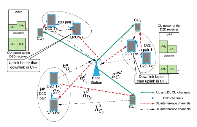
Figure 1: Overall Network model

In conclusion, no existing work provides a joint channel assignment and power allocation scheme that satisfies all of the following requirements: (i) considers both uplink and downlink spectrum;(ii) accounts for uncertainties in CSI and thus obtains a robust resource allocation solution;and (iii) D2D pairs can simultaneously operate on more than one cellular channel, which is of special interest in areas of high CU density. This paper addresses the above mentioned limitations and provides the following research contributions:

• We propose a joint uplink and downlink resource allocation scheme, which assigns both power and channel resources to D2D pairs and CUs. The objective of this scheme is to maximize the total network rate while maintaining fairness in the channel assignment among the D2D pairs. In addition, the scheme also allows assigning multiple channels to each D2D pair. Moreover, the proposed scheme also accounts for uncertainties in the channels by introducing probabilistic constraints that guarantee the desired outage probabilities.

• We propose a computationally efficient solution for the resulting problem, even though it is a mixed integer non-convex optimization problem, which involves exponential complexity to compute the optimal solution. We first show that without loss of optimality, the overall problem can be decomposed into several power allocation subproblems and a channel assignment problem. The solution of the power allocation sub-problems in the case of perfect CSI is obtained in closed form, whereas in the scenario of imperfect CSI, a quadratic transformation and alternating optimization methods are proposed. The proposed algorithms can be implemented centrally at the BS.

• We also propose decentralized algorithms that reduce the computational load at the BS by solving each power allocation sub-problem in parallel at the corresponding D2D pair. Moreover, some of the computations for the channel assignment problem are also performed by the D2D pairs. Furthermore, the communication can start immediately after the first iteration without waiting for the algorithms convergence.

• We provide convergence guarantees to stationary points for all of our algorithms and we show linear convergence rate for some of the considered cases and sub-linear convergence rates for other cases.

• Extensive simulations are also presented to demonstrate the advantages of the proposed method as compared to current state-of-the-art alternatives.

II System Model and Problem Statement

Consider an underlay D2D communication scenario in which both uplink and downlink cellular channels are accessible to D2D pairs. In the following description, we describe the considered communication scenario, which is also depicted in Fig. 1.

Cellular network configuration: We consider a cell (or sector) of a cellular network in which the serving BS and the associated CUs communicate via $N_{C}^{(u)}$ uplink and $N_{C}^{(d)}$ downlink channels, respectively. Considering the worst case underlay scenario, we assume, without loss of generality, a fully loaded cellular communication scenario in which all uplink and downlink channels are assigned to CUs. For notational convenience, the set of CUs communicating in respective uplink and downlink channels are indexed as $\mathcal{C}^{(u)}$ = $\left\{1,...,N_{C}^{(u)}\right\}$ and $\mathcal{C}^{(d)}$ = $\left\{1,...,N_{C}^{(d)}\right\}$.

D2D communication configuration: Next, we assume that $N_{D}$ D2D pairs $\left(\right.$indexed by $j\in\mathcal{D}$ = $\left.\left\{1,...,N_{D}\right\}\right)$ desire to communicate over the aforementioned downlink and uplink channels in an underlay configuration, i.e., simultaneously on the same uplink and downlink channels assigned to the CUs. The assignment of uplink or downlink channels to D2D pairs is represented by the indicator variables $\{\beta^{(u)}_{i,j}\}$ and $\{\beta^{(d)}_{i,j}\}$, respectively, where $j$ denotes D2D pair ($j\in\mathcal{D}$) and $i$ denotes either uplink or downlink channel $\left(i\in\mathcal{C}^{(u)}~{}or~{}\mathcal{C}^{(d)}\right)$. Here $\beta^{(u)}_{i,j}=1$ or $\beta^{(d)}_{i,j}=1$ when the $j$-th D2D pair accesses the $i$-th uplink or downlink channel. In order to improve throughput of the D2D pairs, we further assume that each D2D pair can access multiple channels at the same time. However, in-order to restrict interference among D2D pairs, we assume that each channel can be used by at most one D2D pair, this can be expressed as $\sum\limits_{j=1}^{N_{D}}\beta^{(u)}_{i,j}\leq 1,~{}\sum\limits_{j=1}^{N_{D}}\beta^{(d)}_{i,j}\leq 1~{}\forall~{}i$. In addition, to reduce hardware complexity, we further assume that each D2D pair can have access to multiple channels in either downlink or uplink spectrum band [23, 24], which can be expressed as $\sum\limits_{i=1}^{N_{C}^{(u)}}\beta^{(u)}_{i,j}\times\sum\limits_{i=1}^{N_{C}^{(d)}}\beta^{(d)}_{i,j}=0,~{}\forall j$.

Communication channels: First, we define channel gains in the uplink access. Let $g^{(u)}_{C_{i}}$ denote the channel gain from the $i$-th CU to the BS and $h^{(u)}_{C_{i,j}}$ denote the channel gain of the interference link from the $i$-th CU to the $j$-th D2D pair receiver. Similarly, let $g_{D_{j}}$ denote the channel gain between transmitter and receiver of the $j$-th D2D pair and $h^{(u)}_{D_{j}}$ denote the channel gain of the interference link from the transmitter of the $j$-th D2D pair to the BS. Next, for downlink access, let $g^{(d)}_{C_{i}}$ denote the channel gain from the BS to the $i$-th CU and $h^{(d)}_{C_{j}}$ denote the channel gain of the interference link from the BS to the $j$-th D2D pair. Finally, let $h^{(d)}_{D_{j,i}}$ denote the channel gain of the interference link from the transmitter of the $j$-th D2D pair to the $i$-th CU. Here we assume that the interference channel gains affecting the CUs are estimated with minimum cooperation from the CUs; thus, gains of these interference links are assumed to be modeled as random variables, denoted respectively by $\tilde{h}^{(u)}_{C_{i,j}}$ and $\tilde{h}^{(d)}_{D_{j,i}}$. Finally, additive noise observed in individual channels is assumed to have a known power $N_{0}$. Note that the noise and all channel gains are assume to be frequency flat to simplify the notations; however, the proposed scheme carries over immediately to the frequency selective scenario.

Transmit power constraints: Considering the limited power available at the mobile devices, the transmit power of the $j$-th D2D pair when assigned to the $i$-th uplink or downlink channel, denoted as $P^{(u)}_{D_{j,i}}$ and $P^{(d)}_{D_{j,i}}$ is constrained as $0\leq P^{(u)}_{D_{j,i}}\leq P_{D_{max}},~{}0\leq P^{(d)}_{D_{j,i}}\leq P_{D_{max}}$. Similarly, the transmit power of the CU on the $i$-th uplink channel and of the BS on the $i$-th downlink channels are constrained, respectively, as $0\leq P^{(u)}_{C_{i}}\leq P^{(u)}_{C_{max}}$ and $0\leq P^{(d)}_{C_{i}}\leq P^{(d)}_{C_{max}}$. Note that $P^{(u)}_{C_{max}},~{}P^{(d)}_{C_{max}},~{}$and$~{}P_{D_{max}}$ are assumed to be the same for all CUs and D2D pairs to simplify the notations, however, once again the proposed scheme carries over immediately to the scenario where they are different.

Achievable rates: Here, we first present the achievable rates for D2D underlay communication on downlink channels and then extend our discussion for underlay on uplink channels. Let $R^{(d)}_{C_{i,j}}$ and $R^{(d)}_{D_{j,i}}$ denote the rate of the $i$-th CU and of the $j$-th D2D pair when sharing the downlink channel, which are respectively given as:

$$\begin{array}[]{ll}R^{(d)}_{C_{i,j}}=\log_{2}\left(1+\dfrac{P^{(d)}_{C_{i}}g^{(d)}_{C_{i}}}{N_{0}+P^{(d)}_{D_{j,i}}\tilde{h}^{(d)}_{D_{j,i}}}\right),~{}R^{(d)}_{D_{j,i}}=\log_{2}\left(1+\dfrac{P^{(d)}_{D_{j,i}}g_{D_{j}}}{N_{0}+P^{(d)}_{C_{i}}{h}^{(d)}_{C_{j}}}\right).\end{array}$$

When the $i$-th CU does not share the downlink channel, the achievable rate denoted by $R^{(d)}_{C_{i,0}}$ is given as:

$$R^{(d)}_{C_{i,0}}=\log_{2}\left(1+\dfrac{P^{(d)}_{C_{\max}}g^{(d)}_{C_{i}}}{N_{0}}\right).$$

Thus, the gain in rate when the $i$-th CU shares channel with the $j$-th D2D pair can be stated as, $v^{(d)}_{i,j}=R^{(d)}_{C_{i,j}}+R^{(d)}_{D_{j,i}}-R^{(d)}_{C_{i,0}}$. Finally, the overall network rate in the downlink can be stated as:

$$R^{(d)}(\bm{B}^{(d)},\mathbb{p_{C}}^{(d)},\bm{p_{D}}^{(d)})=\sum_{i\in\mathcal{C}^{(d)}}\left[\sum_{j\in\mathcal{D}}\beta^{(d)}_{i,j}v^{(d)}_{i,j}+R^{(d)}_{C_{i,0}}\right].$$ (1)

where $\bm{B}^{(d)}\triangleq[\beta_{i,j}^{(d)}],~{}\mathbb{p_{C}}^{(d)}\triangleq[P_{C_{1}}^{(d)},P_{C_{2}}^{(d)},\dots,P_{C_{N_{C}}}^{(d)}]^{T},~{}\bm{P_{D}}^{(d)}\triangleq[P_{D{ji}}^{(d)}]$.
Similarly, the achievable rates in the uplink channels when sharing the $i$-th CU uplink channel with the $j$-th D2D pair can be expressed as:

$$\begin{array}[]{ll}R^{(u)}_{C_{i,j}}=\log_{2}\left(1+\dfrac{P^{(u)}_{C_{i}}g^{(u)}_{C_{i}}}{N_{0}+P^{(u)}_{D_{j,i}}{h}^{(u)}_{D_{j}}}\right),~{}R^{(u)}_{D_{j,i}}=\log_{2}\left(1+\dfrac{P^{(u)}_{D_{j,i}}g_{D_{j}}}{N_{0}+P^{(u)}_{C_{i}}\tilde{h}^{(u)}_{C_{i,j}}}\right).\end{array}$$

The achievable rates in the uplink channels without sharing the $i$-th CU uplink channel, the rate gain, as well as the total rate due to underlay uplink communications can be easily expressed by replacing the superscripts $(d)$ by $(u)$ in the above equations.

Quality of Service (QoS) requirements: In order to have a successful communication at a receiver node, a minimum signal to interference plus noise (SINR) ratio requirement is imposed in the problem formulation. Thus, for the $i$-th CU in the uplink/downlink sharing channel with the $j$-th D2D pair, the instantaneous SINR $\eta_{C_{i,j}}^{(u)}\geq\eta^{(u)}_{C_{\min}}$ and $\eta_{C_{i,j}}^{(d)}\geq\eta^{(d)}_{C_{\min}}$, where $\eta^{(u)}_{C_{\min}}$ and $\eta^{(d)}_{C_{\min}}$ are the minimum desired SINR for the CU in uplink and donwlink, respectively. Similarly, for the $j$-th D2D pair, the instantaneous SINR $\eta_{D_{i},j}^{(u)}\geq\eta_{D_{\min}}$, where $\eta_{D_{\min}}$ is the minimum desired SINR for D2D pairs in both uplink and downlink. Note thatin order to simplify the notation $\eta^{(u)}_{C_{\min}},~{}\eta^{(d)}_{C_{\min}},~{}$and$~{}\eta_{D_{\min}}$ are also assumed to be the same for all CUs and D2D pairs; however, the scheme carries over immediately to the scenario where they are different.
Since the computations of the SINR for the $j$-th D2D pair sharing channel with the $i$-th uplink CU involve the random interference channel gain $\tilde{h}^{(u)}_{C{i,j}}$, the minimum SINR requirement can be expressed in terms of a probabilistic constraint as follows:

$$Pr\{\eta_{D_{i,j}}^{(u)}\geq\eta^{(u)}_{D_{min}}\}\geq 1-\epsilon~{}~{}~{}~{}\forall i\in\mathcal{C}^{(u)},~{}~{}\forall j\in\mathcal{D},$$

where $\epsilon$ is the maximum allowed outage probability. Similarly, the minimum SINR requirement for the $i$-th downlink CU sharing channel with the $j$-th D2D pair can be expressed in terms of a probabilistic constraint as follows:

$$Pr\{\eta_{C_{i,j}}^{(d)}\geq\eta^{(d)}_{C_{min}}\}\geq 1-\epsilon~{}~{}~{}~{}\forall i\in\mathcal{C}^{(d)},~{}~{}\forall j\in\mathcal{D}.$$

Fairness in channel assignment to D2D pairs: Let $m_{j}$ denotes the number of channels assigned to the $j$-th D2D pair.

$$m_{j}=\sum\limits_{i_{u}=1}^{N^{(u)}_{C}}\sum\limits_{i_{d}=1}^{N^{(d)}_{C}}\left(\beta^{(u)}_{i_{u},j}+\beta^{(d)}_{i_{d},j}\right).$$

Then inspired by the fairness definition in [10], the fairness of a channel allocation can be expressed in terms of a normalized variance from a specified reference assignment $m_{0}$ as follows:

$$\delta =\dfrac{{\dfrac{1}{N_{D}}\sum\limits_{j=1}^{N_{D}}(m_{j}-m_{0})^{2}}}{m_{0}^{2}}$$ (2)

Problem statement: Given all $g^{(u)}_{C_{i}},~{}g^{(d)}_{C_{i}},~{}g_{D_{j}},~{}h^{(u)}_{D_{j}},~{}h^{(d)}_{C_{j}},~{}\text{the statistical distribution of }\tilde{h}^{(u)}_{C_{i,j}}$, and $\tilde{h}^{(d)}_{D_{j,i}}~{}\forall i,j$, as well as $N_{0}$, $\eta^{C}_{\min}$, $\eta^{D}_{\min}$, $P_{C_{\max}}$, and $P_{D_{\max}}$, the goal is to choose $\beta_{i,j}^{(d)},\beta_{i,j}^{(u)},~{}P_{D_{ji}}^{(d)},~{}P_{D_{ji}}^{(u)}$, $~{}P_{C_{i}}^{(d)},~{}P_{C_{i}}^{(u)}$ to maximize the overall rate of the D2D pairs and CUs while ensuring fairness among the multiple D2D pairs and preventing detrimental interference to CUs.

We consider two different scenarios of D2D pairs communicating over underlay downlink/ uplink channels: ($\mathbf{S1}$) D2D pairs are pre-organized into uplink and downlink groups based on hardware limitations to communicate in either uplink or downlink channels; ($\mathbf{S2}$) The assignment of the D2D pairs to either uplink or downlink channels is also part of the optimization problem. Furthermore, in order to reduce the computation load on the BS, we also propose decentralized solution for both the scenarios. In both the scenarios, we analyze both perfect and imperfect CSI cases.

III Separate Downlink and Uplink Resource Allocation

Recall from Sec. II that each D2D pair is allowed to operate either in the uplink or in the downlink, but not in both simultaneously. For the sake of the exposition, this section assumes that the assignment of D2D pairs to either the uplink or downlink is given. Sec. IV will extend the approach presented in this section to the scenario where such an assignment is not given and therefore becomes part of the resource allocation task. Thus, there are two pre-organized sets of D2D pairs, namely $\mathcal{D}^{(d)}$ and $\mathcal{D}^{(u)}$, intending to communicate in downlink and uplink channels, respectively. Since the D2D pairs are already pre-organized in two separate sets, the joint resource allocation problems simplifies to solving two separate but similar problems: (i) allocating downlink resources to the D2D pairs in the set $\mathcal{D}^{(d)}$; (ii) and allocating uplink resources to the D2D pairs in the set $\mathcal{D}^{(u)}$. Thus, due to the similarity of the two problems, we only discuss the donwlink resource allocation in this section. Since it introduces no ambiguity and simplifies the notation, in this section, we will drop the superscript denoting uplink and downlink.

III-A Resource Allocation Under Perfect CSI (PCSI)

Here, we first analyze the ideal scenario in which perfect CSI can be exploited to maximize the aggregate throughput of both the D2D pairs and CUs while ensuring fairness among D2D pairs. To this end, our problem formulation is as follows:

$$\mathop{\text{maximize}}_{\bm{B},\mathbb{p_{C}},\bm{P_{D}}}\quad R(\bm{B},\mathbb{p_{C}},\bm{P_{D}})-\gamma\delta(\bm{B})$$ (3a)

subject to $$\beta_{i,j}\in\{0,1\},~{}\forall~{}i,j,~{}\sum\limits_{j=1}^{N_{D}}\beta_{i,j}\leq 1~{}\forall~{}i,,$$ (3b)

$$0\leq P_{C_{i}}\leq P_{C_{max}},~{}\forall~{}i,~{}0\leq P_{D_{ji}}\leq P_{D_{max}},~{}\forall~{}i,j,$$ (3c)

$$~{}\dfrac{P_{C_{i}}g_{C_{i}}}{N_{0}+P_{D_{ji}}h_{D_{j,i}}}\geq\eta^{C}_{min}\text{ if }\beta_{ij}=1,~{}\forall~{}i,j,$$ (3d)

$$\dfrac{P_{D_{ji}}g_{Dj}}{N_{0}+P_{C_{i}}h_{C_{j}}}\geq\eta^{D}_{min}\text{ if }\beta_{ij}=1,~{}\forall~{}i,j,$$ (3e)

where the total rate $R(\bm{B},\bm{p_{C}},\bm{P_{D}})$ is given by (1). The fairest resource assignment in this framework corresponds to uniformly distributing the $N_{C}$ available channels equally over the D2D pairs ($m_{0}:={N_{C}}/{N_{D}}$). Substituting $m_{0}$ in (2), the fairness in channel allocation $\delta(\bm{B})$ can be expressed as:

$$\delta(\bm{B}) =\dfrac{N_{D}}{N_{C}^{2}}{\sum\limits_{j=1}^{N_{D}}\left(\sum\limits_{i=1}^{N_{C}}\beta_{i,j}-N_{C}/N_{D}\right)^{2}}$$ (4)

We consider a user-selected regularization parameter $\gamma>0$ in (3a) to balance the rate-fairness trade-off. In general, the highest rate is achieved when all channels are assigned only to D2D pairs with good communications conditions. The fairness in the assignment needs to be enforced by adding a term in the objective function that penalizes unfair assignments.

The optimization problem in (3) is a non-convex mixed-integer problem and obtaining the optimal solution of such a combinatorial problem will incur an exponential complexity. Next, we show that problem (3) can be decomposed into two steps without loosing optimality: (S1) power allocation; and (S2) channel assignment.

First, consider solving (3a) w.r.t. $\mathbb{p}_{C}$ for fixed $\bm{P}_{D}$ and $\bm{B}$. It can be seen from (1) that the objective of (3) can be written as $\sum_{i\in\mathcal{C}}\sum_{j\in\mathcal{D}}\beta_{i,j}$ $v_{i,j}(P_{C_{i}},P_{D_{ji}})$ plus some terms that do not depend on $[P_{C_{i}}]$. Notice that an equivalent problem can be obtained by replacing $P_{C_{i}}$ with an artificial auxiliary variable $P_{C_{i,j}}$ in each term $\beta_{i,j}v_{i,j}(P_{C_{i}},P_{D_{ji}})$ and further enforcing the constraint $P_{C_{i,1}}=P_{C_{i,2}}=\ldots=P_{C_{i,N_{D}}}$ for each $i$. Then, the modified objective can be expressed as $\sum_{i\in\mathcal{C}}\sum_{j\in\mathcal{D}}\beta_{i,j}v_{i,j}(P_{C_{i,j}},P_{D_{ji}})$ plus terms that do not depend on $[P_{C_{i,j}}]$. Similarly, we can replace $P_{C_{i}}$ with $P_{C_{i,j}}$ in (3d)-(3e) and also in (3c) with $0\leq P_{C_{i,j}}\leq P_{C_{max}}\,\forall i,j$ and the resulting problem will be equivalent to (3). Thus, except for the recently introduced equality constraints, the objective and the constraints will only depend on at most one of the $P_{C_{i,j}}$ for each $i$, specifically the one with $\beta_{i,j}=1$. Hence, the equality constraint $P_{C_{i,1}}=\ldots=P_{C_{i,N_{D}}}$ can be dropped without loss of optimality. To recover the optimal $[P^{*}_{C_{i}}]$ in (3) from the optimal $[P^{*}_{C_{i,j}}]$ , one just needs to find, for each $i$, the value of $j$ such that $\beta_{i,j}=1$ and set $P_{C_{i}}^{*}=P_{C_{i,j}}^{*}$. If no such $j$ exists, i.e. $\beta_{i,j}=0~{}~{}\forall j$, then channel $i$ is not assigned to any D2D pair and the BS can transmit with maximum power $P_{C_{i}}=P_{C_{\max}}$. Similarly, without loss of optimality, we can also remove the condition “if $\beta_{i,j}=1$” from (3d)-(3e). Thus, the resulting problem can be expressed as:

$$\mathop{\text{maximize}}_{\bm{B},\bm{P_{C}},\bm{P_{D}}}\quad \sum\limits_{i\in\mathcal{C}}\sum\limits_{j\in\mathcal{D}}\left[\beta_{i,j}v_{i,j}(P_{C_{ij}},P_{D_{ji}})\right]-\gamma\delta(\bm{B})$$ (5a)

subject to $$\beta_{i,j}\in\{0,1\},~{}\forall~{}i,j,~{}\sum\limits_{j=1}^{N_{D}}\beta_{i,j}\leq 1\,~{}\forall~{}i,$$ (5b)

$$0\leq P_{C_{ij}}\leq P_{C_{max}},~{}~{}0\leq P_{D_{ji}}\leq P_{D_{max}},~{}\forall~{}i,j,$$ (5c)

$$\dfrac{P_{C_{ij}}g_{C_{i}}}{N_{0}+P_{D_{ji}}h_{D_{j,i}}}\geq\eta^{C}_{min},~{}\dfrac{P_{D_{ji}}g_{D_{j}}}{N_{0}+P_{C_{ij}}h_{C_{j}}}\geq\eta^{D}_{min},~{}\forall~{}i,j$$ (5d)

where $\bm{P_{C}}\triangleq[P_{C_{ij}}]$.

Since $\bm{B}$ is binary, (5) can now be decoupled without loss of optimality into a power allocation problem and a channel allocation problem. Furthermore, the optimization of (5) with respect to $\bm{P_{C}}$ and $\bm{P_{D}}$ (power allocation problem) decouples across $i$ and $j$ into the $N_{C}N_{D}$ sub-problems of the form:

$$\mathop{\text{maximize}}_{P_{C_{ij}},P_{D_{ji}}}\quad v_{i,j}(P_{C_{ij}},P_{D_{ji}})$$ (6)

subject to $$0\leq P_{C_{ij}}\leq P_{C_{max}},\quad 0\leq P_{D_{ji}}\leq P_{D_{max}},$$

$$\dfrac{P_{C_{ij}}g_{C_{i}}}{N_{0}+P_{D_{ji}}h_{D_{j,i}}}\geq\eta^{C}_{min},\quad\dfrac{P_{D_{ji}}g_{D_{j}}}{N_{0}+P_{C_{ij}}h_{C_{j}}}\geq\eta^{D}_{min},$$

which should be solved $\forall i\in\mathcal{C},\forall j\in\mathcal{D}$. This power allocation subproblem coincides with the one arising in [16, 29, 30], which can be solved in closed-form, since the solution should be on the borders of the feasibility region (defined by the constraints in (6)). More specifically, as illustrated in Fig. 2, it can be shown that for any point $(P^{\prime}_{C_{ij}},P^{\prime}_{D_{ji}})$ in the interior of the feasibility region, there exist a point $(\alpha P^{\prime}_{C_{ij}},\alpha P^{\prime}_{D_{ji}})$ at the border segments that has a higher objective value. Moreover, since the objective function is convex on the border segments, and therefore the optimal point is one of the intersection points of the border segments (the maximum of a convex function is achieved at the borders of the feasibility region).

Figure 2: Power feasibility region

Once (6) has been solved $\forall i\in\mathcal{C},\forall j\in\mathcal{D}$, it remains to substitute the optimal values $[v^{*}_{i,j}]_{i,j}$ into (5) and then minimize with respect to $\bm{B}$. If (6) is infeasible for a given $(i,j)$, then we set its optimal value to $v^{*}_{i,j}=-\infty$. The resulting channel assignment subproblem can be expressed as follows,

$$\mathop{\text{maximize}}\limits_{\bm{B}}\quad \sum_{i\in\mathcal{C}}\sum\limits_{j\in\mathcal{D}}\beta_{i,j}v^{*}_{i,j}-\gamma\delta(\bm{B}),$$ (7)

subject to $$\beta_{i,j}\in\{0,1\}~{}\forall i,j,\quad\sum\limits_{j\in\mathcal{D}}\beta_{i,j}\leq 1~{}\forall i.$$

Notice that problem (7) is an integer program of combinatorial nature. Finding an exact solution using exhaustive search would be computationally unaffordable and time consuming for a sufficiently large $N_{C}N_{D}$. Thus, considering the practicality of implementation, we compute a sub-optimal solution with a smaller computational complexity by relaxing the integer constraint $\beta_{i,j}\in\{0,1\}$ of (7) with $\beta_{i,j}\in[0,1]$.

The resulting problem is convex and the resulting solutions $[\tilde{\beta}_{i,j}]$ can be efficiently obtained e.g. through projected gradient descent (PDG) [31]. Discretizing the solution $[\tilde{\beta}_{i,j}]$ to such a problem is expected to yield an approximately optimal optimum of (7). For this discretization we consider two approaches: (i) for every $i$, set $\beta_{i,j}=1$ if $j=\operatorname*{arg\,max}_{j}\tilde{\beta}_{i,j}$. (ii) for each $i$, consider a random variable $J_{i}$ taking values $1,\ldots,N_{D}$ with probabilities $P(J_{i}=j)=\tilde{\beta}_{i,j}/\sum\limits_{j\in\mathcal{D}}\tilde{\beta}_{i,j}$. Then, we generate a certain set of realizations of $\{J_{i}\}$ and form the corresponding set of matrices $\{\bm{B}$}, whose $(i,j)$-th entry is 1 if $J_{i}=j$ and 0 otherwise. Finally, we evaluate the objective of (7) for all these realizations and select the realization with the highest objective value.

III-B Resource Allocation Under Imperfect CSI (ICSI)

In this scenario, we assume having infrequent and limited measurements from the CUs and the D2D pairs that are used in estimating the channel gain from the D2D pairs to the CUs. This will create uncertainty in the available CSI. Thus, in this case, the objective function and the SINR constraints in (5) involve a random channel gain $\tilde{h}_{D_{j,i}}$ for the interference link from the $j$-th D2D pair to the $i$-th CU.

First, the SINR constraint (5d) can be replaced with a probabilistic constraint to guarantee a maximum outage probability $\epsilon$ which can be expressed as:

$$\Pr\left\{\eta_{ij}^{c}\triangleq\dfrac{P_{C_{ij}}g_{C_{i}}}{N_{0}+P_{D_{ji}}\tilde{h}_{D_{j,i}}}\geq\eta^{c}_{min}\right\}\geq 1-\epsilon.$$ (8)

The probabilistic constraint in (8) can be expressed in closed form for a given statistical distribution of $\tilde{h}_{D_{ji}}$. Generally, (8) is equivalent to:$\Pr\left\{\tilde{h}_{D_{j,i}}\leq\dfrac{P_{C_{ij}}g_{C_{i}}-\eta^{c}_{min}N_{0}}{P_{D_{ji}}\eta^{c}_{min}}\right\}\geq 1-\epsilon$, or, equivalently

$$\dfrac{P_{C_{ij}}g_{C_{i}}}{N_{0}+P_{D_{ji}}\text{F}^{-1}_{\tilde{h}_{D_{j,i}}}(1-\epsilon)}\geq\eta^{c}_{min},$$ (9)

where $\text{F}^{-1}_{\tilde{h}}(1-\epsilon)$ is the inverse cumulative distribution function (CDF) function for $\tilde{h}$ evaluated at $1-\epsilon$. We will consider exponential, Gaussian, Chi-squared, and log-normal distributions in the following sections, since they are the most common in wireless communication environment.

Next, focussing on the objective function, we consider two approaches: (i) expected network rate maximization; and (ii) minimum network rate maximization.

III-B1 Expected Network Rate Maximization (ERM)

One possibility is to replace the objective of (3) with its expectation. To this end, notice that $\mathbb{E}_{\mathbb{\tilde{h}}}\{R\}=\sum_{i\in\mathcal{C}}\left[\sum_{j\in\mathcal{D}}\beta_{i,j}\mathbb{E}_{\tilde{h}_{D_{j,i}}}\{v_{i,j}\}+R_{C_{i,0}}\right]$, and from the definition of $v_{ij}$:

$$\mathbb{E}_{\tilde{h}_{D_{j,i}}}\{v_{i,j}(P_{C_{ij}},P_{D_{ji}})\}=\mathbb{E}_{\tilde{h}_{D_{j,i}}}\{R_{C_{i,j}}(P_{C_{ij}},P_{D_{ji}})\}+R_{D_{j,i}}(P_{C_{ij}},P_{D_{ji}})-R_{C_{i,0}}.$$

Since the expectation of $R_{C_{i,j}}(P_{C_{ij}},P_{D_{ji}})$ is not tractable analytically for the aforementioned distributions, one can replace the expectation by the first-order or the second-order Taylor series approximations around the mean of ${\tilde{h}_{D_{j,i}}}$.

Calculation method	Deviation $|\hat{v}_{i,j}-\bar{v}_{i,j}|/\bar{v}_{i,j}$ between the approximation $\hat{v}_{i,j}$ and the Monte-Carlo average $\bar{v}_{i,j}$ for $10^{6}$ samples
	First order	Second order
Exponential ($\bar{h}_{C_{ij}}=0.2$)	0.6499%	0.1392%
Gaussian ($\bar{h}_{C_{ij}}=0.2,~{}\mathop{\textrm{Var}}\left\{h_{C_{ij}}\right\}=0.01$)	0.8934%	0.1062%
Chi-squared ($\bar{h}_{C_{ij}}=0.2,~{}\mathop{\textrm{Var}}\left\{h_{C_{ij}}\right\}=0.01$)	0.8930%	0.1058%
Log-normal ($\bar{h}_{C_{ij}}=0.2,~{}\mathop{\textrm{Var}}\left\{h_{C_{ij}}\right\}=0.01$)	0.6898%	0.0991%

TABLE II: Expectation approximations

Table II shows the comparison between first-order and second-order approximations in the computation of $\mathbb{E}_{\tilde{h}_{D_{j,i}}}\{v_{ij}\}$, where we can note that both approximations are very close to the Monte-Carlo averages in all the tested distributions. Besides, the first-order approximation results in an error comparable to the second-order approximation. Because of this reason and the higher simplicity, we consider the first-order approximation. Moreover, the resulting expectation is the so-called certainty equivalence approximation, which is an extensively adopted approximation in stochastic optimization [31]. Using the expectation of the first-order Taylor approximation in the objective function along with aforementioned constraints in (9) leads to a problem similar to (6), which can be solved in closed form as before.

III-B2 Minimum guaranteed rate maximization (MRM)

In this approach, the criterion to maximize is the network rate exceeded for a (1-$\epsilon$) portion of the time. First, we define the $(1-\epsilon)$-guaranteed SINR for the $i$-th CU when sharing the channel with the $j$-th D2D pair as $\eta^{\epsilon}_{C_{i,j}}$ such that $\text{Pr}\{\eta_{C_{i,j}}>\eta_{C_{i,j}}^{\epsilon}\}=1-\epsilon$. Next, we define $v^{\epsilon}_{ij}=\log(1+\eta^{\epsilon}_{C_{i,j}})+\log(1+\eta_{D_{i,j}})-R_{C_{i,0}}$ and $R^{\epsilon}=\sum_{i\in\mathcal{C}}\left[\sum_{j\in\mathcal{D}}\beta_{i,j}v^{\epsilon}_{i,j}+R_{C_{i,0}}\right]$, siilar to the work in [32]. The resource allocation problem can be formulated as (3) with $R$ replaced by $R^{\epsilon}$ and the SINR constraints replaced by (9). Proceeding as in Sec. III-A, such a problem is equivalent to (5) with $v_{ij}$ replaced with $v^{\epsilon}_{ij}$ and the SINR constraints replaced by (9). Similar steps can also be followed to decouple the problem into power assignment and channel allocation subproblems. Up to a constant term, the objective of the power allocation sub-problems can be expressed as:

$$F_{0}\triangleq\log_{2}\left(1+\dfrac{P_{C_{ij}}g_{C_{i}}}{N_{0}+P_{D_{ji}}\text{F}^{-1}_{\tilde{h}_{{D_{j,i}}}}(1-\epsilon)}\right)+\log_{2}\left(1+\dfrac{P_{D_{ji}}g_{D_{j}}}{N_{0}+P_{C_{ij}}h_{C_{j}}}\right)$$ (10)

where $\eta^{\epsilon}_{C_{i,j}}$ is expressed in closed-form similar to (8) for a given statistical distribution of $\tilde{h}_{D_{j,i}}$. The rest of this section proposes a method to solve this power allocation subproblem.

This objective function is non-convex. However, it can be seen as a sum of log-functions of “concave-over-convex” fractions. Given this structure, fractional programming techniques [33, 34] constitute a natural fit.To take the fractions outside the log-functions, we introduce the slack variables $\mathbb{z}\triangleq[z_{1},~{}z_{2}]^{T}$. The resulting power assignment problem can be rewritten as follows:

$$\mathop{\text{maximize}}_{P_{C_{ij}},P_{D_{ji}},\bm{z}}\quad \log_{2}\left(1+z_{1}\right)+\log_{2}\left(1+z_{2}\right)$$ (11a)

subject to $$z_{1}\leq\dfrac{P_{C_{ij}}g_{C_{i}}}{N_{0}+P_{D_{ji}}\text{F}^{-1}_{\tilde{h}_{D_{j,i}}}(1-\epsilon)},\quad z_{2}\leq\dfrac{P_{D_{ji}}g_{D_{j}}}{N_{0}+P_{C_{ij}}h_{C_{j}}}$$ (11b)

$$0\leq P_{C_{ij}}\leq P_{C_{max}},\quad 0\leq P_{D_{ji}}\leq P_{D_{max}},$$ (11c)

$$\dfrac{P_{C_{ij}}g_{C_{i}}}{N_{0}+P_{D_{ji}}\text{F}^{-1}_{\tilde{h}_{D_{j,i}}}(1-\epsilon)}\geq\eta^{C}_{min},\quad\dfrac{P_{D_{ji}}g_{D_{j}}}{N_{0}+P_{C_{ij}}h_{C_{j}}}\geq\eta^{D}_{min}.$$ (11d)

The optimal values of the auxiliary variables occur when the inequalities hold with equality ($z_{1}^{*}={P_{C_{ij}}g_{C_{i}}}/{N_{0}+P_{D_{ji}}\text{F}^{-1}_{\tilde{h}_{D_{j,i}}}(1-\epsilon)},~{}z_{2}^{*}={P_{D_{ji}}g_{D_{j}}}/{N_{0}+P_{C_{ij}}h_{C_{j}}}$). Let us consider the Lagrangian of (11) with respect to the first two inequalities:

$$L(\bm{p},\bm{z},\bm{\lambda}) =\log_{2}\left(1+z_{1}\right)+\log_{2}\left(1+z_{2}\right)-\lambda_{1}\left(z_{1}-\dfrac{P_{C_{ij}}g_{C_{i}}}{N_{0}+P_{D_{ji}}\text{F}^{-1}_{\tilde{h}_{D_{j,i}}}(1-\epsilon)}\right)$$

$$-\lambda_{2}\left(z_{2}-\dfrac{P_{D_{ji}}g_{D_{j}}}{N_{0}+P_{C_{ij}}h_{C_{j}}}\right)$$ (12)

A stationary point of $L$ with respect to $\bm{z}$ is achieved when ${\partial L}/{\partial\bm{z}}=\bm{0}$. This leads to $\lambda_{1}=1/(1+z_{1}),~{}\lambda_{2}=1/(1+z_{2})$. Substituting $\bm{z}^{*}$ in these equations yields:

$$\lambda_{1}^{*}=\dfrac{N_{0}+P_{D_{ji}}\text{F}^{-1}_{\tilde{h}_{D_{j,i}}}(1-\epsilon)}{P_{C_{ij}}g_{C_{i}}+N_{0}+P_{D_{ji}}\text{F}^{-1}_{\tilde{h}_{D_{j,i}}}(1-\epsilon)},\quad\lambda_{2}^{*}=\dfrac{N_{0}+P_{C_{ij}}h_{C_{j}}}{P_{D_{ji}}g_{D_{j}}+N_{0}+P_{C_{ij}}h_{C_{j}}}$$ (13)

Substituting $\mathbf{\lambda}^{*}$ in (III-B2), we obtain:

$$\mathop{\text{maximize}}_{P_{C_{ij}},P_{D_{ji}},\bm{z}}\quad F_{1}\triangleq L(\bm{p},\bm{z},\bm{\lambda}^{*})=\log_{2}\left(1+z_{1}\right)+\log_{2}\left(1+z_{2}\right)-z_{1}$$ (14)

$$+\dfrac{(1+z_{1})P_{C_{ij}}g_{C_{i}}}{P_{C_{ij}}g_{C_{i}}+N_{0}+P_{D_{ji}}\text{F}^{-1}_{\tilde{h}_{D_{j,i}}}(1-\epsilon)}-z_{2}+\dfrac{(1+z_{2})P_{D_{ji}}g_{D_{j}}}{P_{D_{ji}}g_{D_{j}}+N_{0}+P_{C_{ij}}h_{C_{j}}}$$

subject to $$\eqref{eq:d2rmaxp},~{}\eqref{eq:d2rSINR}$$

Finally, to handle the fractions in the objective function, we use the quadratic transformation in [33, 34], to transform each fraction into a substitute concave expression. Then, we obtain:

$$\mathop{\text{maximize}}_{P_{C_{ij}},P_{D_{ji}},\bm{z},\bm{y}}\quad F_{2}\triangleq\log_{2}\left(1+z_{1}\right)+\log_{2}\left(1+z_{2}\right)-z_{1}+2y_{1}\sqrt{(1+z_{1})P_{C_{ij}}g_{C_{i}}}$$ (15)

$$-y_{1}^{2}(P_{C_{ij}}g_{C_{i}}+N_{0}+P_{D_{ji}}\text{F}^{-1}_{\tilde{h}_{D_{j,i}}}(1-\epsilon))-z_{2}+2y_{2}\sqrt{(1+z_{2})P_{D_{ji}}g_{D_{j}}}$$

$$-y_{2}^{2}(P_{D_{ji}}g_{D_{j}}+N_{0}+P_{C_{ij}}h_{C_{j}})$$

subject to $$\eqref{eq:d2rmaxp},~{}\eqref{eq:d2rSINR},$$

where $\mathbf{y}\triangleq[y_{1}~{}y_{2}]^{T}$ are the auxiliary variables given by the quadratic transformation.

This problem is then solved by alternating maximization with respect to the individual $y_{1},y_{2}$, $P_{C_{ij}},P_{D_{ji}}$ variables. At each step, all iterates can be obtained in closed form by taking the partial derivative with respect to each variable and setting it to $0$, and projecting the solution onto the feasible set. The overall iteration can be expressed as:

$$z_{1}^{[k+1]}= \dfrac{P_{C_{ij}}^{[k]}g_{C_{i}}}{N_{0}+P_{D_{ji}}^{[k]}\text{F}^{-1}_{\tilde{h}_{D_{j,i}}}(1-\epsilon)},~{}\quad z_{2}^{[k+1]}=\dfrac{P_{D_{ji}}^{[k]}g_{D_{j}}}{N_{0}+P_{C_{ij}}^{[k]}h_{C_{j}}}$$ (16a)

$$y_{1}^{[k+1]} =\dfrac{\sqrt{(1+z_{1}^{[k+1]})P_{C_{ij}}^{[k]}g_{C_{i}}}}{P_{C_{ij}}^{[k]}g_{C_{i}}+N_{0}+P_{D_{ji}}^{[k]}\text{F}^{-1}_{\tilde{h}_{D_{j,i}}}(1-\epsilon)},~{}y_{2}^{[k+1]}=\dfrac{\sqrt{(1+z_{2}^{[k+1]})P_{D_{ji}}^{[k]}g_{D_{j}}}}{P_{D_{ji}}^{[k]}g_{D_{j}}+N_{0}+P_{C_{ij}}^{[k]}h_{C_{j}}}$$ (16b)

$$P_{C_{ij}}^{[k+1]} =\text{Proj}_{\mathcal{S}_{1}^{[k]}}\left(\dfrac{(y_{1}^{[k+1]})^{2}(1+z_{1}^{[k+1]})g_{C_{i}}}{((y_{1}^{[k+1]})^{2}g_{C_{i}}+(y_{2}^{[k+1]})^{2}h_{C_{j}})^{2}}\right)$$ (16c)

$$P_{D_{ji}}^{[k+1]} =\text{Proj}_{\mathcal{S}_{2}^{[k+1]}}\left(\dfrac{(y_{2}^{[k+1]})^{2}(1+z_{2}^{[k+1]})g_{D_{j}}}{((y_{2}^{[k+1]})^{2}g_{D_{j}}+(y_{1}^{[k+1]})^{2}\text{F}^{-1}_{\tilde{h}_{D_{j,i}}}(1-\epsilon))^{2}}\right)$$ (16d)

where $k$ is the iteration index, $\text{Proj}_{\mathcal{A}}(\bm{*})$ is a projection of $\bm{*}$ onto the set $\mathcal{A}$; $S_{1}^{[k]}\triangleq\{P_{C_{ij}}:(P_{C_{ij}},P_{D_{ji}}^{[k]})$ satisfy (11c) and (11d)}, and $S_{2}^{[k+1]}\triangleq\{P_{D_{ji}}:(P_{C_{ij}}^{[k+1]},P_{D_{ji}})$ satisfy (11c) and (11d)}. Next, we show that, with this alternating optimization solution, $|F_{0}(P_{C_{ij}}^{[k]},P_{D_{ji}}^{[k]})-F_{0}(P_{C_{ij}}^{*},P_{D_{ji}}^{*})|$ converges in the order $\mathcal{O}(k^{-\alpha})$, for some $\alpha>0$).

Theorem 1.

Let $\{\mathbf{p}^{[k]}\}_{k\in\mathbb{N}_{+}}$ be the sequence generated by (16) with $\mathbf{p}^{[k]}\triangleq[P_{D_{ji}}^{[k]}~{}P_{C_{ij}}^{[k]}]^{T}$. Then, (i) $\lim\limits_{k\rightarrow\infty}\mathbf{p}^{[k]}=\bar{\mathbf{p}}$ where $\bar{\mathbf{p}}$ is a stationary point of (15), and (ii) $|\mathbf{p}^{[k]}-\bar{\mathbf{p}}|\leq Ck^{-(1-\theta)/(2\theta-1)}$ for some $C>0$.

Proof.

see Appendix A ∎

After solving the power allocation subproblems in both the ERM or MRM cases, a channel allocation problem similar to (7) will arise, and a similar solution based on integer relaxation can be used. Algorithm 1 highlights the operation of the separate resource allocation method with all the previously discussed cases, with $\bm{B}^{(d)}(k),\bm{B}^{(u)}(k),\bm{P}_{C}^{(d)}(k),\bm{P}_{D}^{(d)}(k),\bm{P}_{D}^{(u)}(k),$ $\bm{P}_{C}^{(u)}(k)$ are the values of each variable at the $k$-th iteration, and $\bf P_{D_{j}}^{(d)},\bf P_{C_{j}}^{(d)}$ are the $j$-th columns of $\bf P_{D}^{(d)},\bf P_{C}^{(d)}$ matrices. Since the objective function of the channel allocation problem is Lipschitz smooth, this algorithm will converge as $\mathcal{O}(1/k)$ (as shown in Theorem 3.7 in [35]) in the case of PCSI and ICSI-ERM with $\mathcal{O}(N_{C}^{2}N_{D})$ computational operations per iteration. Similarly, in the case of ICSI-MRM, the algorithm will converge as $\mathcal{O}(1/k+k^{-\alpha})$ for some $\alpha>0$, with similar computations per iteration.

Algorithm 1 Centralized Separate Resource Allocation

1:Initialize: $\bm{B}^{(d)}(0),\bm{B}^{(u)}(0),\bm{P}_{C}^{(d)}(0),\bm{P}_{D}^{(d)}(0),\bm{P}_{D}^{(u)}(0),$ $\bm{P}_{C}^{(u)}(0),k=0$

2:for all $j\in\mathcal{D}^{(d)}$ do $\triangleright$ Power Assignment in downlink to find: $\bf P_{D_{j}}^{(d)^{*}},\bf P_{C_{j}}^{(d)^{*}}$.

3:     if PCSI mode OR ICSI-ERM mode then

4:         BS uses the closed-form power allocation in Sec. III-A.

5:     else$\triangleright$ ICSI-MRM mode

6:         BS applies (16) iteratively until convergence.

7:     end if

8:end for

9:repeat

10:     $k=k+1$

11:     BS uses the PGD algorithm to calculate: $\bm{B}^{(d)}(k)$

12:until $\bm{B}^{(d)}$ converges

13:…$\triangleright$ The same for uplink

14:BS discretize $\bm{B}^{(d)},\bm{B}^{(u)}$.

IV Joint Uplink and Downlink Resource Allocation

In this section, we analyze the scenario in which D2D pairs are assigned uplink or downlink channels on the basis of instantaneous channel conditions, i.e., the algorithm itself generates a decision on the set of D2D pairs communicating in the uplink or the downlink while maximizing the aggregate network throughput. Problem (5) can be extended to the joint uplink and downlink resource allocation case by considering the following modified objective function:

$$\mathop{\text{maximize}}\limits_{\bm{B},\bm{P_{C}},\bm{P_{D}}}\sum\limits_{i\in\mathcal{C}}\sum\limits_{j\in\mathcal{D}}[\beta^{(u)}_{i,j}U^{(u)}_{i,j}(P^{(u)}_{C_{ij}},P^{(u)}_{D_{ji}})+\beta^{(d)}_{i,j}U^{(d)}_{i,j}(P^{(d)}_{C_{ij}},P^{(d)}_{D_{ji}})]-\gamma\delta_{J}(\bm{B}^{(u)},\bm{B}^{(d)}),$$ (17)

where $U^{(u)}_{i,j}(P^{(u)}_{C_{ij}},P^{(u)}_{D_{ji}})$ and $U^{(d)}_{i,j}(P^{(d)}_{C_{ij}},P^{(d)}_{D_{ji}})$ are general utility functions for the uplink and downlink selected depending on the working conditions (PCSI, ICSI-ERM, or ICSI-MRM), which are set to either the rate gain or the expected rate gain or the minimum rate gain defined in Sec. III. In addition, the constraints must also be extended to take into account both up-link and down-link communications.

Here, we redefine a joint unfairness metric $\delta_{J}$ for joint resource allocation in uplink and downlink. Let $N_{D}$ be the number of D2D pairs and let $N_{C}^{(u)}$ and $N_{C}^{(d)}$ be the total number of channels available in the uplink and downlink respectively. A D2D pair is allowed to communicate in either the downlink or uplink ($\sum\limits_{i\in\mathcal{C}^{(d)}}\beta^{{(d)}}_{i,j}\times\sum\limits_{i\in\mathcal{C}^{(u)}}\beta^{{(u)}}_{i,j}=0~{}\forall j$). The fairest possible assignment is the one assigning $m_{0}=(N_{C}^{(u)}+N_{C}^{(d)})/N_{D}=N_{C}^{(u)}/N_{D}+N_{C}^{(d)}/N_{D}\triangleq m_{0}^{(u)}+m_{0}^{(d)}$ to each D2D pair. Similarly to Sec. II, we can adopt the following fairness metric:

$$\delta_{J}(\bm{B}^{{(u)}},\bm{B}^{{(d)}})=\dfrac{\sum\limits_{j\in\mathcal{D}}(m_{j}-m_{0})^{2}}{m_{0}^{2}~{}N_{D}}=\dfrac{1}{m_{0}^{2}~{}N_{D}}\sum\limits_{j\in\mathcal{D}}\left(\sum\limits_{i\in\mathcal{C}^{(u)}}\beta^{{(u)}}_{i,j}+\sum\limits_{i\in\mathcal{C}^{(d)}}\beta^{{(d)}}_{i,j}-m_{0}^{(u)}-m_{0}^{(d)}\right)^{2}$$

$$=\dfrac{(m_{0}^{(u)})^{2}}{m_{0}^{2}}\delta(\bm{B}^{{(u)}})-\dfrac{2}{m_{0}^{2}~{}N_{D}}\sum\limits_{j\in\mathcal{D}}\left(m_{0}^{(d)}\sum\limits_{i\in\mathcal{C}^{(u)}}\beta^{{(u)}}_{i,j}\right)+\dfrac{(m_{0}^{(d)})^{2}}{m_{0}^{2}}\delta(\bm{B}^{{(d)}})$$

$$-\dfrac{2}{m_{0}^{2}~{}N_{D}}\sum\limits_{j\in\mathcal{D}}\left(m_{0}^{(u)}\sum\limits_{i\in\mathcal{C}^{(d)}}\beta^{{(d)}}_{i,j}\right)+\dfrac{2m_{0}^{(u)}m_{0}^{(d)}}{m_{0}^{2}}$$ (18)

The resulting optimization problem is now given by:

$$\mathop{\text{maximize}}\limits_{\bm{B}^{{(u)}},\bm{B}^{{(d)}},\bm{P}^{{(u)}},\bm{P}^{{(d)}}} \sum\limits_{i\in\mathcal{C}}\sum\limits_{j\in\mathcal{D}}\left[\beta^{{(u)}}_{i,j}U^{{(u)}}_{i,j}(P^{{(u)}}_{C_{ij}},P^{{(u)}}_{D_{ji}})+\beta^{{(d)}}_{i,j}U^{{(d)}}_{i,j}(P^{{(d)}}_{C_{ij}},P^{{(d)}}_{D_{ji}})\right]-\gamma\delta_{J}(\bm{B}^{{(u)}},\bm{B}^{{(d)}}),$$ (19a)

s.t. $$\beta^{{(u)}}_{i,j}\in\{0,1\},~{}~{}\beta^{{(d)}}_{i,j}\in\{0,1\},\quad~{}\forall~{}i,j$$ (19b)

$$\sum\limits_{j\in\mathcal{D}}\beta^{{(d)}}_{i,j}\leq 1,~{}~{}\sum\limits_{j\in\mathcal{D}}\beta^{{(u)}}_{i,j}\leq 1,\quad~{}\forall~{}i$$ (19c)

$$\left(\sum\limits_{i\in\mathcal{C}^{(d)}}\beta^{{(d)}}_{i,j}\right)\times\left(\sum\limits_{i\in\mathcal{C}^{(u)}}\beta^{{(u)}}_{i,j}\right)=0,\quad~{}\forall~{}j$$ (19d)

$$\text{UL/DL power and SINR constraints similar to }\eqref{eq:probeq}$$ (19e)

Similar to (5), this problem can further be decomposed into power and channel problems as before without loss of optimality. The power allocation problems are of the form of (6) or (11) depending on the available CSI (PCSI or ICSI) and the selected criteria (ERM or MRM).

IV-A Resource Allocation under Perfect CSI (PCSI)

In this case, the objective function in (19) becomes deterministic and the decomposition of the problem leads to a similar independent power allocation problem for each pair ($i,j$) as in III-A, which can be solved in closed form and obtain the optimal $U^{{(u)}^{*}}_{i,j},~{}U^{{(d)}^{*}}_{i,j}$.
The channel allocation problem becomes:

$$\mathop{\text{maximize}}\limits_{\bm{B}^{{(u)}},\bm{B}^{{(d)}}} \sum\limits_{i\in\mathcal{C}}\sum\limits_{j\in\mathcal{D}}[\beta^{{(u)}}_{i,j}U^{{(u)}^{*}}_{i,j}+\beta^{{(d)}}_{i,j}U^{{(d)}^{*}}_{i,j}]-\gamma\delta_{2}(\bm{B}^{{(u)}},\bm{B}^{{(d)}}),$$ (20a)

s.t. $$\eqref{eq:jc1},~{}\eqref{eq:jc2},~{}\text{and}~{}\eqref{eq:jc3}.$$ (20b)

Relaxing the problem by ignoring the constraints (19d) and converting the binary constraints in (19b) to linear constraints as in sec. III-A, leads to a convex problem with linear constraints. This problem can also be solved using PGD, since it is differentiable with linear constraints. Finally, the obtained solution needs to be discretized and projected onto to the set defined by (19d). We propose obtaining a binary solution in the same way used for discretizing (7). Afterwards, for each pair, we evaluate the objective function with the pair assigned to either uplink or downlink; we then select the one which has a higher objective function. After that, we then repeat the channel assignment with the pair removed from the deselected spectrum. The whole process is then repeated until all pairs are assigned. In general, there are many ways to project a solution into the constraints in (19d), however, one cannot guarantee optimallity since (20) has been relaxed.

IV-B Resource Allocation under Imperfect CSI (ICSI)

The power allocation subpoblems here will be similar to Sec. III-B and will adhere to similar solutions. The channel allocation problem is similar to Sec. IV-A and will follow the same solutions. Algorithm 2 describes the operation of the joint resource allocation methods. As shown in Sec. III, this algorithm will converge as $\mathcal{O}(1/k)$ in the case of PCSI and ICSI-ERM, and in the case of ICSI-MRM, the algorithm will converge as $\mathcal{O}(1/k+k^{-\alpha})$ for some $\alpha>0$, with $\mathcal{O}(N_{C}^{2}N_{D})$ computational operations per iteration in all cases.

Algorithm 2 Centralized Joint Resource Allocation

1:Initialize: $\bm{B}^{(d)}(0),\bm{B}^{(u)}(0),\bm{P}_{C}^{(d)}(0),\bm{P}_{D}^{(d)}(0),\bm{P}_{D}^{(u)}(0),$ $\bm{P}_{C}^{(u)}(0),k=0$

2:

3:for all $j\in\mathcal{D}$ do $\triangleright$ Power assignment in both downlink and uplink to find: $\bf P_{D_{j}}^{(d)^{*}},\bf P_{C_{j}}^{(d)^{*}},\bf P_{D_{j}}^{(u)^{*}},\bf P_{C_{j}}^{(u)^{*}}$.

4:     if PCSI mode OR ICSI-ERM mode then

5:         BS uses the closed-form power allocation in Sec. III-A.

6:     else$\triangleright$ ICSI-MRM mode

7:         BS applies (16) iteratively until convergence.

8:     end if

9:end for

10:repeat

11:     $k=k+1$

12:     BS uses the PGD algorithm to calculate: $\bm{B}^{(d)}(k),\bm{B}^{(u)}(k)$

13:until $\bm{B}^{(d)},\bm{B}^{(u)}$ converges

14:BS discretize $\bm{B}^{(d)},\bm{B}^{(u)}$.

V Decentralized Algorithms

In order to limit dependence of D2D communication on BS together with reducing BS’s computational load, we also consider decentralizing the resource allocation algorithms. Furthermore, our aim is to start the communication immediately after the first iteration without waiting for convergence of the algorithm. Since the power assignment subproblems are independent, they can be solved entirely by the D2D pairs. To decompose the channel allocation problem, let $G$ be the objective function of (7). $G$ and its gradient can be express as:

$$G=\text{vec}(\bm{V})^{T}\text{vec}(\bm{B})-k_{1}\|\bm{B}^{T}\bm{1}-k_{2}\bm{1}\|^{2},$$ (21a)

$$\nabla G=\bm{V}-2k_{1}(\bm{1}\bm{1}^{T}\bm{B}-k_{2}\bm{1}\bm{1}^{T}),$$ (21b)

where $\bm{V}\triangleq[v_{ij}]$, and $k_{1}$ and $k_{2}$ are constants. Notice that, the channel allocation problem can not be directly decomposed into disjoint subproblems for each D2D pair, due to the quadratic term in (21). Nevertheless, the gradient is linear in $\bm{B}$, thus, the descent part of the channel allocation algorithm can be directly decomposed and each D2D pair can perform an optimization step over its corresponding part, without loss of optimality. Only the projection and the discretization have to be performed centrally at the BS.

V-A Separate Uplink and Downlink Resource Allocation

Algorithm 3 below describes how this scenario can be solved in a decentralized manner. The BS initializes the power assignment vectors and the channel allocation matrices, and broadcasts them. Each D2D pair perform a step of the power allocation algorithm suitable for the network operation scenario (i.e. closed form for PCSI or ICSI-ERM or the alternating minimization in (16) for ICSI-MRM). Then, each D2D pair updates its vectors of the channel allocations ($\bm{B}^{{(d)}}_{j},\bm{B}^{{(u)}}_{j}$) by performing a gradient step. Each D2D pair then sends its channel allocation vectors along with the calculated power values to the BS. Then, the BS assembles all the vectors of the channel allocation matrices and projects them into a feasible solution and resends them to all D2D pairs. The BS and D2D pairs uses these calculated powers and channel assignments for communications. These steps are then repeated until all variables converge. Algorithm 3 will also converge as $\mathcal{O}(1/k)$ in the case of PCSI and ICSI-ERM, and as $\mathcal{O}(1/k+k^{-\alpha})$ for some $\alpha>0$ for the case of ICSI-MRM. However, $\mathcal{O}(N_{C}^{2})$ computational operations per iteration are performed by each D2D pair, and $\mathcal{O}(N_{C}N_{D})$ computational operations per iteration are performed by the BS with $2N_{C}N_{D}$ variables exchanged between the D2D pairs and the BS in every iteration.

Algorithm 3 Decentralized Separate Resource Allocation

1:Initialize: $\bm{B}^{{(d)}}(0),\bm{B}^{{(u)}}(0),\bm{P}_{C}^{{(d)}}(0),\bm{P}_{D}^{{(d)}}(0),\bm{P}_{D}^{{(u)}}(0),$ $\bm{P}_{C}^{{(u)}}(0),k=0$

2:for all $j\in\mathcal{D}^{{(d)}}$ do

3:     BS sends $\bf B_{j}^{{(d)}}(0),\bf P_{C_{j}}^{{(d)}}(0),\bf P_{D_{j}}^{{(d)}}(0)$ to D2D pair $j$.

4:end for

5:for all $j\in\mathcal{D}^{{(u)}}$ do

6:     BS sends $\bf B_{j}^{{(u)}}(0),\bf P_{C_{j}}^{{(u)}}(0),\bf P_{D_{j}}^{{(u)}}(0)$ to D2D pair $j$.

7:end for

8:repeat

9:     $k=k+1$

10:     for all $j\in\mathcal{D}^{{(d)}}$ do $\triangleright$ Find: $\bf P_{D_{j}}^{{(d)}}(k),\bf P_{C_{j}}^{{(d)}}(k),\bf B_{j}^{{(d)}}(k)$.

11:         if PCSI mode OR ICSI-ERM mode then

12:              D2D pair $j$ uses the closed-form power allocation in Sec. III-A.

13:         else$\triangleright$ ICSI-MRM mode

14:              D2D pair $j$ applies (16) for a single iteration.

15:         end if

16:         D2D pair $j$ sends $\bf P_{C_{j}}^{{(d)}}(k)$ to the BS.

17:         D2D pair $j$ applies a single iteration of the PGD algorithm and sends $\bf B_{j}^{{(d)}}(k)$ to the BS.

18:     end for

19:     …$\triangleright$ The same for uplink

20:     BS projects $\bm{B}^{{(d)}}(k)$ and $\bm{B}^{{(u)}}(k)$ and sends each column to the corresponding D2D pair.

21:until $\bm{B}^{{(d)}},B^{{(u)}},\bm{P}_{C}^{{(d)}},\bm{P}_{D}^{{(d)}},\bm{P}_{D}^{{(u)}},\bm{P}_{C}^{{(u)}}$ converges

V-B Joint Uplink and Downlink Resource Allocation

Algorithm 4 below describes how this scenario can be solved in a decentralized manner. The BS initializes the power assignment vectors and the channel allocation matrices, and broadcasts them. Each D2D pair performs a step of the power allocation method suitable for the operation scenario followed by updating the vectors of the channel allocation ($\bm{B}^{{(d)}}_{j},\bm{B}^{{(u)}}_{j}$) using a gradient step. Then, the BS assembles all the vectors of the channel allocation matrices and projects them into a feasible solution and broadcasts them to all D2D pairs. The BS and D2D pairs uses these calculated powers and channel assignments for communications. These steps are then repeated until all variables converge. Algorithm 4 has the same convergence and computational behaviour as Algorithm 3.

Algorithm 4 Decentralized Joint Resource Allocation

1:Initialize: $\bm{B}^{{(d)}}(0),\bm{B}^{{(u)}}(0),\bm{P}_{C}^{{(d)}}(0),\bm{P}_{D}^{{(d)}}(0),\bm{P}_{D}^{{(u)}}(0),$ $\bm{P}_{C}^{{(u)}}(0),k=0$

2:for all $j\in\mathcal{D}$ do

3:     BS sends $\bf B_{j}^{{(d)}}(0),\bf B_{j}^{{(u)}}(0),\bf P_{C_{j}}^{{(d)}}(0),\bf P_{D_{j}}^{{(d)}}(0),\bf P_{D_{j}}^{{(u)}}(0),\bf P_{C_{j}}^{{(u)}}(0)$ to D2D pair $j$.

4:end for

5:repeat

6:     $k=k+1$

7:     for all $j\in\mathcal{D}$ do $\triangleright$ Find: $\bf P_{D_{j}}^{{(d)}}(k),\bf P_{C_{j}}^{{(d)}}(k),\bf P_{D_{j}}^{{(u)}}(k),\bf P_{C_{j}}^{{(u)}}(k),\bf B_{j}^{{(d)}}(k),\bf B_{j}^{{(u)}}(k)$.

8:         if PCSI mode OR ICSI-ERM mode then

9:              D2D pair $j$ uses the closed-form power allocation in Sec. III-A.

10:         else$\triangleright$ ICSI-MRM mode

11:              D2D pair $j$ applies (16) for a single iteration.

12:         end if

13:         D2D pair sends $P_{C_{j}}^{{(d)}}(k),P_{C_{j}}^{{(u)}}(k)$ to the BS.

14:         D2D pair applies a single iteration of the PGD algorithm and sends $\bf B_{j}^{{(d)}}(k),\bf B_{j}^{{(u)}}(k)$ to the BS.

15:     end for

16:     BS projects $\bm{B}^{{(d)}}(k),\bm{B}^{{(u)}}(k)$ and sends each column to the corresponding D2D pair.

17:until $\bm{B}^{{(d)}},\bm{B}^{{(u)}},\bm{P}_{C}^{{(d)}},\bm{P}_{D}^{{(d)}},\bm{P}_{D}^{{(u)}},\bm{P}_{C}^{{(u)}}$ converges

VI Simulations

We consider a simulation scenario with a single cell of radius 500 m. In this cell, CUs and D2D transmitters are located uniformly at random. The D2D receivers are located uniformly at random in a 5 m radius circle centered at their respective transmitter. A path-loss model with exponent $\alpha=2$ is used in the calculation of all channel gains. The random channel gains are calculated by applying an exponential random distribution around an average calculated from the path-loss model. $N_{C}=10,N_{D}=10$ were used in the experiments with Monte-Carlo averages carried over $10,000$ different realizations.

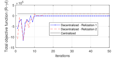
Figure 3: Rate of convergence

Fig. 3 shows the convergence results for the Decentralized Algorithm 4 with imperfect CSI (ICSI)-minimum guaranteed rate maximization (MRM) compared to the Centralized Algorithm 2 with ICSI-MRM of a simulation scenario with two realizations for $\gamma=50$. It shows that the decentralized algorithm converges in a relatively small number of iterations. Similar behaviour is also observed when comparing the the Decentralized Algorithm 3 compared to the Centralized Algorithm 1. The obtained decentralized solutions, in general, are not identical to the centralized solution but it are very close. This is as expected because the alternating optimization for the power allocation and the binary channel allocation problem might have different solutions based on the initialization and the projection, since it is not convex.

Figs. 4, 5, and 6 shows comparisons of Algorithm 3 in the cases of perfect CSI (PCSI), ICSI-expected rate maximization (ERM) and ICSI-MRM, compared with the previous state-of-the-art methods in [27]. Additionally, we assumed all D2D pairs will use only downlink spectrum.The achieved rate of the PCSI case is the highest, as expected, since it ignores the probabilistic constraints and only uses the average channel gains. The cases of ICSI-ERM and ICSI-MRM achieve the second and third rate respectively. The method in [27] achieves the lowest rate since it does not allow assigning multiple channels to a D2D pair. The rates of all methods, except the PCSI case, grow with the allowed outage probability $\epsilon$. However, the fairness of the method in [27] is the best for the same reason (D2D pair can not access multiple channels). All cases of Algorithm 3 achieve relatively similar fairness, with the order of ICSI-MRM, ICSI-ERM, and PCSI from the second best to the forth respectively. The achieved outage probabilities of [27] and case ICSI-ERM are exactly equal to the allowed outage probability $\epsilon$, since the achieved optimal power assignment lies in the border of the feasibility region in both methods. Case ICSI-MRM achieves a better outage probability than the desired $\epsilon$ with the corresponding gap increasing when $\epsilon$ increases; this can be caused by the fact that the power allocation algorithm converges to a local optima rather than the global one, and the number of feasible local optimums increases when expanding the feasibility set. The PCSI case achieves a very high outage probability, which is fixed, regardless of the value of $\epsilon$.

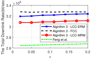
Figure 4: Total Rate vs. $\epsilon$

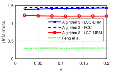
Figure 5: Fairness vs. $\epsilon$

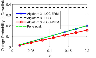
Figure 6: Outage Probability vs. $\epsilon$

Fig. 7 shows comparisons between algorithms 3 and 4 in a ICSI-ERM case and ICSI-MRM case. Algorithm 3 is tested in the following scenarios; all D2D pairs in downlink, all D2D pairs in uplink, half D2D pairs in downlink and half in uplink. The results shows that uplink is generally better than downlink, as expected, due to the lower interference in uplink caused by the lower maximum transmitting power and the possibly longer distances between the D2D pairs and the CUs. Moreover, distributing users among both uplink and downlink achieves significantly higher data rates, with Algorithm 4 achieves the highest rates, since the distribution of users is also optimized.

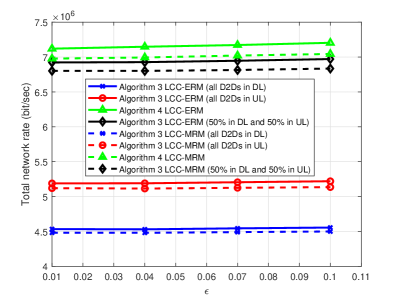
Figure 7: The total network rate (UL+DL) vs. $\epsilon$

VII Conclusion

This paper formulates a joint channel allocation and power assignment problem in underlay D2D communications. This problem aims at maximizing the total network rate while keeping the fairness among the D2D pairs. It also allows assigning multiple channels to each D2D pair. Furthermore, it assigns both downlink and uplink resources either jointly or separately. Moreover, it considers uncertainties in the CSI by including probabilistic SINR constraints to guarantee the desired outage probability. Although this problem is a non-convex mixed-integer problem, we solve it in a computationally efficient manner by convex relaxation, quadratic transformation and alternating optimization techniques. Additionally, decentralized algorithms to solve this problem are also presented in this paper. Numerical experiment show that our algorithms achieve substantial performance improvements as compared to the state-of-the-art.

Appendix A Proof of Theorem 1

First, let us define an equivalent problem to (15) as follows:

$$\mathop{\text{maximize}}_{\bm{p},\bm{z},\bm{y}}\quad F_{2}(\bm{p},\bm{z},\bm{y})$$ (22a)

subject to $$\eqref{eq:d2rmaxp},~{}\eqref{eq:d2rSINR},$$

$$z_{1}=\dfrac{P_{C_{ij}}g_{C_{i}}}{N_{0}+P_{D_{ji}}\text{F}^{-1}_{\tilde{h}_{D_{j,i}}}(1-\epsilon)},~{}\quad z_{2}=\dfrac{P_{D_{ji}}g_{D_{j}}}{N_{0}+P_{C_{ij}}h_{C_{j}}},$$ (22b)

$$y_{1}=\dfrac{\sqrt{(1+z_{1})P_{C_{ij}}g_{C_{i}}}}{P_{C_{ij}}g_{C_{i}}+N_{0}+P_{D_{ji}}\text{F}^{-1}_{\tilde{h}_{D_{j,i}}}(1-\epsilon)},~{}y_{2}=\dfrac{\sqrt{(1+z_{2})P_{D_{ji}}g_{D_{j}}}}{P_{D_{ji}}g_{D_{j}}+N_{0}+P_{C_{ij}}h_{C_{j}}},$$ (22c)

where the additional constraints (22b) and (22c) are obtained from the solutions of (15) in (16a) and (16b) respectively. Since the solution of (15) lies in the feasible set of (22a), both problems are equivalent.

Next, we prove that the limit point $\bar{\mathbf{p}}$ of $\{\mathbf{p}^{[k]}\}_{k\in\mathbb{N}_{+}}$ is a stationary point of (22a). It is shown in Theorem 2.8 in [36] that, for any bounded continuous function that (i) is locally Lipschitz smooth and strongly convex for each block in the feasibility set, (ii) has a Nash point, and (iii) satisfies the Kurdyka Lojasiewicz (KL) property in a neighborhood around a stationary point, the sequence generated by an alternation optimization algorithm with a fixed update scheme initialized in that neighborhood will converge to that stationary point. We will next show that $-F_{2}$ satisfies (i), (ii), and (iii).

A Nash point $\bar{\mathbb{x}}$ for a function $f(\mathbb{x})$ is defined as a block-wise minimizer where $f(\bar{\mathbb{x}}_{1},\dots,\bar{\mathbb{x}}_{i},$ $\dots,\bar{\mathbb{x}}_{s})$ $\leq f(\bar{\mathbb{x}}_{1},\dots,\mathbb{\mathbb{x}}_{i},\dots,\bar{\mathbb{x}}_{s})~{}\forall i$ and $\mathbb{x}=(\mathbb{x}_{1},\mathbb{x}_{2},\dots,\mathbb{x}_{s})$ [36]. Since $F_{2}$ is continuous and the feasible set of (22a) is compact, $F_{2}$ attains a locally optimal point as stated by Weierstrass’ Theorem described in (A.2.7) in [37]. Thus, the function $F_{2}$ has a Nash point. The function $-F_{2}(\mathbf{p},\mathbf{z},\tilde{\mathbf{y}})$ can be shown to be strongly convex and Lipschitz smooth in each variable separately in the bounded feasible set of (22a) ($\partial^{2}F_{2}/\partial z_{1}^{2}=-(1+z_{1})^{-2}-y_{1}\sqrt{P_{C_{ij}}g_{C_{i}}}(1+z_{1})^{-3/2}/2$, $\partial^{2}F_{2}/\partial z_{2}^{2}=-(1+z_{2})^{-2}-y_{2}\sqrt{P_{D_{ji}}g_{D_{i}}}(1+z_{2})^{-3/2}/2$, $\partial^{2}F_{2}/\partial y_{1}^{2}=-2(P_{C_{ij}}g_{C_{i}}+N_{0}+P_{D_{ji}}\text{F}^{-1}_{\tilde{h}_{D_{j,i}}}(1-\epsilon))$, $\partial^{2}F_{2}/\partial y_{2}^{2}=-2(P_{D_{ji}}g_{D_{j}}+N_{0}+P_{C_{ij}}h_{C_{j}})$, $\partial^{2}F_{2}/\partial P_{C_{ij}}^{2}=-y_{1}\sqrt{(1+z_{1})g_{C_{i}}}(P_{C_{ij}})^{-3/2}/2$, $\partial^{2}F_{2}/\partial P_{D_{ji}}^{2}=-y_{2}\sqrt{(1+z_{2})g_{D_{j}}}(P_{D_{ji}})^{-3/2}/2$).

To see that (iii) holds, we use the following definition of the Kurdyka Lojasiewicz (KL) property [36]:

Definition 1.

Kurdyka Lojasiewicz (KL) property: A function $f(\mathbb{x})$ satisfies the KL property at point $\bar{\mathbb{x}}\in\text{dom}(\partial f)$ if $\eta=\dfrac{|f(\mathbb{x})-f(\bar{\mathbb{x}})|^{\theta}}{dist(\mathbb{0},\partial f(\mathbb{x}))}$ is bounded for $0\leq\theta<1$ $\forall\mathbb{x}$ in some neighborhood $U$ of $\bar{\mathbb{x}}$.

We then introduce a lemma as follows:

Lemma 1.

The function $F_{2}(\mathbf{p},\mathbf{z},\mathbf{y})$ satisfies the KL property at any point $\mathbf{p}\in\mathcal{P}$, $\mathbf{z}\in\mathbb{R}^{2}_{+}$ and $\mathbf{y}\in\mathbb{R}^{2}_{+}$, for some $\theta\in[1/2,1)$.

Proof: see Appendix B
Since $F_{2}$ is analytic everywhere, it is also analytic around a stationary point $[\bar{\mathbb{p}},~{}\bar{\mathbb{z}},~{}\bar{\mathbb{y}}]^{T}$ and, consequently, satisfies (iii). Thus the alternation sequence in (16) initialized at any feasible point $\mathbb{p}^{0}$ will converge to the nearest stationary point of $F_{2}$, since $\mathbb{p}^{0}$ is in the neighborhood of the nearest stationary point $\bar{\mathbb{p}}$. Moreover, any stationary point of $F_{2}$ is a stationary point of $F_{0}$ [33, 34]. Thus the sequence $\{\mathbf{p}^{[k]}\}_{k\in N_{+}}$ converges to a stationary point of $F_{0}$.

Next, we prove that $|\mathbf{p}^{[k]}-\bar{\mathbf{p}}|\leq Ck^{-(1-\theta)/(2\theta-1)}$ for some $C>0$. It is shown in theorem 2.9 in [36], for a function $f(\mathbb{x})$ that satisfies Theorem 2.8 in [36] and the KL property for some $\theta\in(1/2,1)$, the update sequence ${\mathbb{x}^{[k]}}$ converges to a stationary point $\bar{\mathbb{x}}$ as $|\mathbb{x}^{[k]}-\bar{\mathbb{x}}|\leq Ck^{-(1-\theta)/(2\theta-1)}$ with a certain $C>0$. Since $F_{2}(\mathbf{p},\mathbf{z},\mathbf{y})$ satisfy the KL property for some $\theta\in(1/2,1)$, the update sequence $\{\mathbf{p}^{k}\}_{k\in N_{+}}$ converges as $|\mathbb{p}^{[k]}-\bar{\mathbb{p}}|\leq Ck^{-(1-\theta)/(2\theta-1)}$ to a stationary point $\bar{\mathbf{p}}$.

Appendix B Proof of Lemma 1

It can be shown that any real analytic function satisfies the KL property for some $\theta\in[1/2,1)$ [36, sec. 2.2]. Next, we need to show that $F_{2}(\mathbf{p},\mathbf{z},\mathbf{y})$ is a real analytic function. A function $f(\mathbb{x})$ is a real analytic function if it is infinitely differentiable and its Taylor series around a point $\mathbb{x}_{0}$ converges to $f(\mathbb{x})$ for $\mathbb{x}$ in some neighbourhood of $\mathbb{x}_{0}$ [38]. To simplify our problem, we first need to consider the following properties of real analytic functions [38]: (i) The sum and product of real analytic functions is a real analytic function. (ii) Any polynomial is a real analytic function. (iii) The composition of real analytic functions is a real analytic function. Exploiting, the first property, it suffices to show that all individual terms in the expression of $F_{2}(\mathbf{p},\mathbf{z},\mathbf{y})$ in (15) are real analytic.

We first show that $\log(\bm{.})$ is real analytic on a positive real argument, i.e., $x\in(0,\infty)$. This can be formally proved by showing that the remainder of the order-n Taylor series expansion of $\log(x)$ centered around a point $c$ goes to zero as $n$ goes to infinity. The Taylor series expansion of $\log(x)$ centered at $c>0$, can be expressed as: $\sum^{\infty}_{n=0}\frac{(-1)^{n}(n-1)!}{n!c^{n}}(x-c)^{n}.$Our objective is to show that above expansion converges to $\log(x)~{}\forall~{}x\in(c/2,3c/2)$. The Lagrange reminder of the Taylor’s series expansion of function $f(x)$ can be expressed as: $R_{n}(x)=\frac{f^{(n+1)}(\zeta)}{(n+1)!}(x-c)^{n+1}$, where, $f^{(n+1)}(.)$ is the $(n+1)$-th derivative of $f$. Substituting $f(\zeta)=\log(\zeta)$, we have $R_{n}(x)=\frac{(-1)^{n}n!}{(n+1)!\zeta^{n+1}}(x-c)^{n+1}$, where, $x,\zeta\in(c/2,3c/2)$. Simplifying further, $|R_{n}(x)|=\frac{1}{(n+1)!}\frac{|x-c|^{n+1}}{|\zeta|^{n+1}}\leq\frac{1}{n+1}$. Thus, $\lim_{n\rightarrow\infty}$, $|R_{n}(x)|\rightarrow 0$. Hence, Taylor’s series expansion of $\log(x)$ centered at $c$ converges to $\log(x)$ on $(c/2,3c/2)$. Further, if $c\rightarrow\infty$, $\log(x)$ is real analytic for $x\in(0,\infty)$. Thus, $\log(1+z_{1})$ and $\log(1+z_{2})$ are real analytic functions for $z_{1},z_{2}>0$.
Next, we consider the following terms of $F_{2}(\mathbf{p},\mathbf{z},\mathbf{y})$: $z_{1};z_{2};y_{1}^{2}(p_{B}g_{D}+N_{0}+P_{D}h_{D});y_{2}^{2}(p_{D}g_{D}+N_{0}+P_{B}h_{B})$. It can be noted that all these terms are positive polynomials. Thus, by the second property, all of these terms are real analytic functions. Finally, for the terms $2y_{1}\sqrt{(1+z_{1})p_{B}g_{B}}$ and $2y_{2}\sqrt{(1+z_{1})p_{B}g_{B}}$, we exploit the first and the third properties. Note that $y_{1},y_{2}$, $(1+z_{1})p_{B}g_{B}$ and $(1+z_{1})p_{B}g_{B}$ are positive polynomials; hence, they are real analytic functions. Thus, we just need to show that the square root is a real analytic function. Let $f(x):\mathbb{R}\rightarrow\mathbb{R}$ be a real analytic function. Then, $\sqrt{f(x)}=e^{\log\left(\sqrt{f(x)}\right)}=e^{\frac{\log(f(x))}{2}}$. Since the composition of real analytic functions is real analytic; given that $e^{(.)}$ is real analytic and $\log(f(x))$ is real analytic for $f(x)>0$; then, we can conclude that $\sqrt{(f(x))}$ is real analytic for $f(x)>0$.

References

• [1] A.B. Ericsson, “Ericsson mobility report,” 2018.
• [2] Cisco Visual Networking, “Ciscoglobal cloud index: forecast and methodology, 2015-2020. white paper,” 2017.
• [3] I. Csiszar and J. Körner, Information theory: coding theorems for discrete memoryless systems, Cambridge University Press, 2011.
• [4] B. Kaufman and B. Aazhang, “Cellular networks with an overlaid device to device network,” in Proc. Asilomar Conf. Sig., Syst., Comput. IEEE, 2008, pp. 1537–1541.
• [5] A. Asadi, Q. Wang, and V. Mancuso, “A survey on device-to-device communication in cellular networks,” IEEE Commun. Surveys Tuts., vol. 16, no. 4, pp. 1801–1819, 2014.
• [6] J. Liu, N. Kato, J. Ma, and N. Kadowaki, “Device-to-device communication in lte-advanced networks: A survey,” IEEE Commun. Surveys Tuts., vol. 17, no. 4, pp. 1923–1940, 2015.
• [7] F. Jameel, Z. Hamid, F. Jabeen, S. Zeadally, and M. A. Javed, “A survey of device-to-device communications: Research issues and challenges,” IEEE Commun. Surveys Tuts., vol. 20, no. 3, pp. 2133–2168, 2018.
• [8] K. Doppler, C. H. Yu, C. B. Ribeiro, and P. Janis, “Mode selection for device-to-device communication underlaying an lte-advanced network,” in Proc. IEEE Wireless Commun., Netw. Conf. IEEE, 2010, pp. 1–6.
• [9] A. H. Sakr, H. Tabassum, E. Hossain, and D. I. Kim, “Cognitive spectrum access in device-to-device-enabled cellular networks,” IEEE Commun. Mag., vol. 53, no. 7, pp. 126–133, 2015.
• [10] C. Xu, L. Song, Z. Han, Q. Zhao, X. Wang, and B. Jiao, “Interference-aware resource allocation for device-to-device communications as an underlay using sequential second price auction,” in Proc. IEEE Int. Conf. Commun. IEEE, 2012, pp. 445–449.
• [11] C. Xu, L. Song, Z. Han, D. Li, and B. Jiao, “Resource allocation using a reverse iterative combinatorial auction for device-to-device underlay cellular networks,” in Proc. IEEE Global Commun. Conf. IEEE, 2012, pp. 4542–4547.
• [12] Y. Chen, B. Ai, Y. Niu, K. Guan, and Z. Han, “Resource allocation for device-to-device communications underlaying heterogeneous cellular networks using coalitional games,” IEEE Trans. Wireless Commun., vol. 17, no. 6, pp. 4163–4176, 2018.
• [13] R. Yin, G. Yu, C. Zhong, and Z. Zhang, “Distributed resource allocation for d2d communication underlaying cellular networks,” in Proc. IEEE Int. Conf. Commun. IEEE, 2013, pp. 138–143.
• [14] R. AliHemmati, B. Liang, M. Dong, G. Boudreau, and S. H. Seyedmehdi, “Power allocation for underlay device-to-device communication over multiple channels,” IEEE Trans. Sig. Info. Process. Netw., vol. 4, no. 3, pp. 467–480, 2017.
• [15] A. Abrardo and M. Moretti, “Distributed power allocation for d2d communications underlaying/overlaying ofdma cellular networks,” IEEE Trans. Wireless Commun., vol. 16, no. 3, pp. 1466–1479, 2017.
• [16] D. Feng, L. Lu, Y. Yuan-Wu, G. Y. Li, G. Feng, and S. Li, “Device-to-device communications underlaying cellular networks,” IEEE Trans. Commun., vol. 61, no. 8, pp. 3541–3551, 2013.
• [17] G. Yu, L. Xu, D. Feng, R. Yin, G. Y. Li, and Y. Jiang, “Joint mode selection and resource allocation for device-to-device communications,” IEEE Trans. Commun., vol. 62, no. 11, pp. 3814–3824, 2014.
• [18] Y. Jiang, Q. Liu, F. Zheng, X. Gao, and X. You, “Energy-efficient joint resource allocation and power control for d2d communications,” IEEE Trans. Veh. Technol., vol. 65, no. 8, pp. 6119–6127, 2016.
• [19] S. Dominic and L. Jacob, “Distributed learning approach for joint channel and power allocation in underlay d2d networks,” in Proc. IEEE Int. Conf. Sig. Process. and Commun. IEEE, 2016, pp. 145–150.
• [20] F. Hajiaghajani, R. Davoudi, and M. Rasti, “A joint channel and power allocation scheme for device-to-device communications underlaying uplink cellular networks,” in IEEE Conf. Comput. Commun. Workshops. IEEE, 2016, pp. 768–773.
• [21] Y. Yuan, T. Yang, H. Feng, and B. Hu, “An iterative matching-stackelberg game model for channel-power allocation in d2d underlaid cellular networks,” IEEE Trans. Wireless Commun., vol. 17, no. 11, pp. 7456–7471, 2018.
• [22] S. Guo, X. Zhou, S. Xiao, and M. Sun, “Fairness-aware energy-efficient resource allocation in d2d communication networks,” IEEE Syst. J., vol. 13, no. 2, pp. 1273–1284, 2018.
• [23] P. Zhao, P. Yu, L. Feng, W. Li, and X. Qiu, “Gain-aware joint uplink-downlink resource allocation for device-to-device communications,” in Proc. IEEE Veh. Technol. Conf. IEEE, 2017, pp. 1–5.
• [24] C. Kai, L. Xu, J. Zhang, and M. Peng, “Joint uplink and downlink resource allocation for d2d communication underlying cellular networks,” in Proc. IEEE Int. Conf. Wireless Commun., Sig. Process. IEEE, 2018, pp. 1–6.
• [25] C. Kai, H. Li, L. Xu, Y. Li, and T. Jiang, “Joint subcarrier assignment with power allocation for sum rate maximization of d2d communications in wireless cellular networks,” IEEE Trans. Veh. Technol., vol. 68, no. 5, pp. 4748–4759, 2019.
• [26] D. Feng, L. Lu, Y. Yuan-Wu, G. Y. Li, G. Feng, and S. Li, “Optimal resource allocation for device-to-device communications in fading channels,” in Proc. IEEE Global Commun. Conf. IEEE, 2013, pp. 3673–3678.
• [27] D. Feng, L. Lu, Y. Yi, G. Y. Li, G. Feng, and S. Li, “Qos-aware resource allocation for device-to-device communications with channel uncertainty,” IEEE Trans. Veh. Technol., vol. 65, no. 8, pp. 6051–6062, Aug 2016.
• [28] Q. Thieu and H. Hsieh, “Outage protection for cellular-mode users in device-to-device communications through stochastic optimization,” in Proc. IEEE Veh. Technol. Conf., May 2015, pp. 1–5.
• [29] A. Gjendemsjo, D. Gesbert, G.E. Oien, and S.G. Kiani, “Optimal power allocation and scheduling for two-cell capacity maximization,” in Int. Symp. on modeling and optimization in mobile, ad hoc and wireless networks. IEEE, 2006, pp. 1–6.
• [30] M. Elnourani, M. Hamid, D. Romero, and B. Beferull-Lozano, “Underlay device-to-device communications on multiple channels,” in Proc. IEEE Int. Conf. Acoust., Speech, Sig. Process. IEEE, 2018, pp. 3684–3688.
• [31] D. P. Bertsekas, Nonlinear Programming, Athena scientific Belmont, 1999.
• [32] M. Elnourani, B. Beferull-Lozano, D. Romero, and S. Deshmukh, “Reliable underlay device-to-device communications on multiple channels,” in Proc. IEEE Int. Workshop Sig. Process. Advances Wireless Commun. IEEE, 2019, pp. 1–5.
• [33] K. Shen and W. Yu, “Fractional programming for communication systems—part i: Power control and beamforming,” IEEE Trans. Sig. Process., vol. 66, no. 10, pp. 2616–2630, May 2018.
• [34] K. Shen and W. Yu, “Fractional programming for communication systems—part ii: Uplink scheduling via matching,” IEEE Trans. Sig. Process., vol. 66, no. 10, pp. 2631–2644, May 2018.
• [35] S. Bubeck et al., “Convex optimization: Algorithms and complexity,” Foundations and Trends® in Machine Learning, vol. 8, no. 3-4, pp. 231–357, 2015.
• [36] Y. Xu and W. Yin, “A block coordinate descent method for regularized multiconvex optimization with applications to nonnegative tensor factorization and completion,” SIAM J. on imaging sciences, vol. 6, no. 3, pp. 1758–1789, 2013.
• [37] D. P. Bertsekas, Convex optimization theory, Athena Scientific Belmont, 2009.
• [38] P.A. Absil, R. Mahony, and B. Andrews, “Convergence of the iterates of descent methods for analytic cost functions,” SIAM J. on Optimization, vol. 16, no. 2, pp. 531–547, 2005.