Probabilistic approach to physical object disentangling

Abstract

Physically disentangling entangled objects from each other is a problem encountered in waste segregation or in any task that requires disassembly of structures. Often there are no object models, and, especially with cluttered irregularly shaped objects, the robot can not create a model of the scene due to occlusion. One of our key insights is that based on previous sensory input we are only interested in moving an object out of the disentanglement around obstacles. That is, we only need to know where the robot can successfully move in order to plan the disentangling. Due to the uncertainty we integrate information about blocked movements into a probability map. The map defines the probability of the robot successfully moving to a specific configuration. Using as cost the failure probability of a sequence of movements we can then plan and execute disentangling iteratively. Since our approach circumvents only previously encountered obstacles, new movements will yield information about unknown obstacles that block movement until the robot has learned to circumvent all obstacles and disentangling succeeds. In the experiments, we use a special probabilistic version of the Rapidly exploring Random Tree (RRT) algorithm for planning and demonstrate successful disentanglement of objects both in 2-D and 3-D simulation, and, on a KUKA LBR 7-DOF robot. Moreover, our approach outperforms baseline methods.

I Introduction

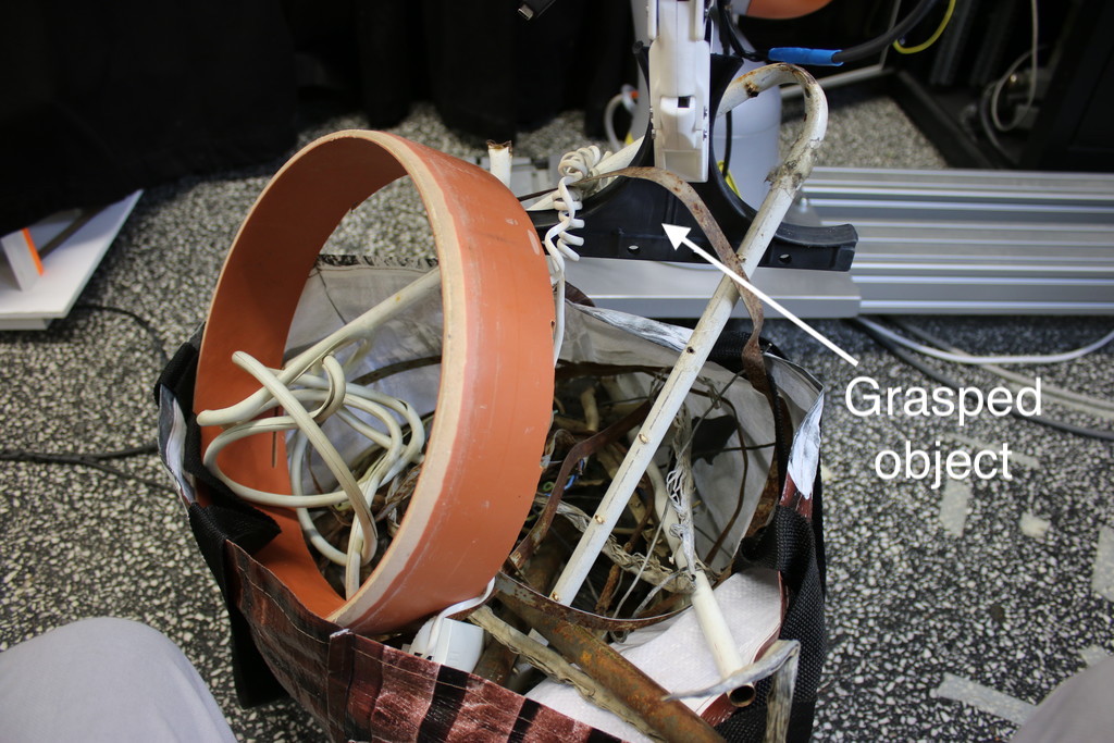
Figure 1: Physical disentangling of an object. (Top) A robot has grasped an object and needs to disentangle the object from other objects. In this case plastic and iron waste. The robot does not get sensory input except its own joint configuration. At each time step the robot plans a path in joint space, tries to execute the path, and collides with an obstacle. The collision is added to a list of collisions. We form a probability map from the task space collisions that tells where the robot will likely collide with obstacles and use the map for choosing paths with low failure probability. (Bottom) Since visualizing the high-dimensional probability map for the real robot is challenging, we show for illustration purposes a sequence of path movements in 2-D task space simulation (we still plan in 7-DOF joint space). A planar multi-link robot uses our probabilistic disentangling approach to choose movements. Blue line denotes planned path, red dots previous collisions, and dark-light colors the probability map where dark color indicates high failure probability. Dark circles depict the real obstacles which are not visible to the robot.

Robots have had a great impact on the manufacturing industry due to their ability to autonomously handle large and heavy objects with high speed and precision. For example, the car manufacturing industry is a typical example for the benefits of robotic automation which is nowadays a key component in the production pipeline of almost every major car manufacturer. Robots have similarly large potential for performing less structured tasks such as sorting and segregating heaps of waste. However, applying robots to such domains is more challenging, because it is no longer sufficient to execute preprogrammed motions due to the uniqueness of the encountered situations. In order to segregate waste, robots need to be able to disentangle objects with unknown shapes. The objects may be entangled in complex ways that are not fully perceivable due to limited sensory information. Furthermore, the effects of disruptive actions, such as pulling a given part of the heap, can not be accurately predicted due to complex dynamical interactions and non-rigid objects.

Albeit challenging, applying robots for waste segregation can be highly rewarding. For example, decommissioning nuclear waste which is inherently dangerous for humans is an ideal task for robots. The Sellafield (UK) nuclear site is the largest nuclear site in Europe, containing 140 tonnes of civil plutonium [1] and 90,000 tonnes of radioactive graphite [2] and the cost of decommissioning was estimated at 47.9 billions GBP in 2015 [3]. Decommissioning includes sorting and segregating 69,600 m³ of mixed intermediate waste, such that waste with high level of radiation can be safely stored in expensive, well-shielded containers, while avoiding unnecessary filling such containers with waste with low level of radiation.

Targeted at this application, we propose a method for autonomous disentangling of waste that is capable to deal with complex, entangled objects based on limited sensory information and that does not require models of the objects or of the dynamical interactions. We assume that the end-effector of the robot has grasped a part of the heap and our goal is to move the end-effector together with the grasped object away from the heap. When such movement succeeds, we consider the object to be disentangled from the heap.

As fully planning such movements a priori is not feasible due to limited sensor data, we adopt an adaptive planning approach that re-plans new movement trajectories such that it avoids motions that are similar to motions that failed in the past due to object entanglement. We therefore learn a probability map over joint configurations that can be used to assess the probability of failing along a given trajectory and use these probabilities as a cost for a variant of the Rapidly exploring Random Tree (RRT [4]) trajectory planner. Our main contribution is an approach that can remove an unknown object from a set of unknown objects when the object configuration prevents a simple movement separating the object from the other objects. We call the process of removing an “entangled” object from other objects “disentangling”.

Our approach does not need any sensory input which is crucial under heavy occlusion, for example, in waste segregation. Moreover, in the nuclear waste scenario, accurate tactile or vision sensors can be hard to use due to potentially high nuclear radiation. Instead of requiring informative sensors, object models, or actually seeing through objects, our approach needs only information about the joint positions of the robot to detect when movement is blocked. In practice, a movement can be blocked either due to the robot being configured to limit the amount of force, as in our experiments, e.g. using impedance control, or a robot physically not being able to exert sufficient force to move through an obstacle.

Our assumptions on the objects is minimal. Due to using a probabilistic formulation of the disentangling task we do not have to assume rigid objects, required by hard constraints, but we instead assign success probabilities to movements and can cope with a (moderately) changing environment: due to never having deterministic probabilities the system has the chance to self-correct its model of the world based on new observations. To summarize:

• We propose a new approach for disentangling objects based on a novel incremental probabilistic path planning formulation.

• Our approach improves the robots knowledge of the environment incrementally until succeeding.

• Due to the probabilistic formulation the approach works in an environment with both rigid and non-rigid unknown objects.

• The approach does not need any sensors but relies solely on joint position information.

II Related Work

In the task of disentangling an unknown object the robot needs to find a motion or path that transports the entangled object out of the entanglement. Path planning in a known environment is a widely studied problem [5, 4, 6, 7] especially in robot motion planning [8] and path planning of mobile robots [9, 10]. Path planning algorithms are often based on the Rapidly explorating Random Tree (RRT) [4] or the Probabilistic Roadmap (PRM) [5]. RRTs iteratively build a tree of joint configurations where the root node corresponds to the start configuration and edges indicate that a direct movement between two configurations is feasible. At each iteration a new joint configuration is sampled and its closest joint configuration within the tree is determined. If a direct connection to the nearest configuration is feasible, the new configuration is added as its child. Once a node inside the tree is sufficiently close to the goal, a path from the start configuration to the goal can be recovered in reverse order by iteratively adding the parent node as via point. PRMs build a graph by sampling random nodes and adding to the graph and then finally finding the shortest path using a graph search method such as Dijkstra’s. Due to the requirements of planning in continuous space in reasonable computation time we adapt an RRT based planning approach but the planner could be exchanged for another.

While the problem of robot manipulator motion planning has been studied, motion planning in unknown environments with unknown obstacles is only little explored, especially for larger than two- or three-dimensional spaces. [11] provides an approach for path planning with a point robot moving in 2D space containing unknown objects. However, the approach in [11] is inherently limited to a 2-D space where the robot can travel around an obstacle and is able to utilize sensory feedback to keep the robot close to the obstacle.

The D*-path planning algorithm [12] which takes inspiration from the A* planning method [13] can adapt to changes in the environment and finds an optimal solution in the limit. However, D*-path planning is limited in practice to discrete state spaces. [14] presents a PRM based approach for path planning and replanning in dynamic environments where the agent repairs its trajectory when new information is received.

Path planning in unknown and dynamic environments has been studied in the context of mobile robot path planning [15, 16]. [17] provides a fuzzy logic based approach for mobile robot path planning and demonstrates the approach in path planning for mobile robots in a 2-D environment. [18] demonstrates a genetic algorithm based approach to path planning for mobile robots in a dynamic unknown environment. [19] utilizes artificial potential fields (APFs) [20] where obstacles repel and goals attract the robot. [21] uses the Bacterial Evolutionary Algorithm (BEA) together with APFs for mobile robot navigation.

In human-robot interaction, the robot often needs to be able to avoid collisions with a hard to predict human. Ideally the robot would not need to make prior assumptions about the human’s location but could learn this online. However, due to the safety requirements human-robot interaction requires in practice (stochastic) models or predictions of human behavior [22]. In physical object disentangling the robot does not usually need to take safety similarly into account and thus prior models are not crucial.

Object disassembly. Disentangling an object away from objects with which it is entangled corresponds to disassembly of an object from a structure. [23] perform path planning for disassembly of complex objects. However, to the best of our knowledge disassembly of unknown objects in an unknown environment has not been performed before. In this paper, our experimental setup focuses on disentangling waste objects but in future work our approach could be applied to disassembly of complex unknown structures.

Waste segregation. Waste segregation is one of the applications motivating our work on object disentangling. State-of-the-art waste segregation relies on classifying and picking up waste that is not entangled [24, 25, 26, 27]. Being able to disentangle different types of waste would allow more efficient reuse of materials. Moreover, being able to disentangle hazardous materials such as nuclear waste [3] can be crucial for safe decommissioning.

III Approach

In this paper, we do not take grasping into account but assume that an object has been already grasped. Grasping is a widely studied problem and there is a multitude of approaches for grasping [28, 29, 30]. Our goal is to disentangle the object. The main research question we investigate is: How to disentangle an unknown object which is firmly planted in the gripper from other unknown objects? To answer this research question we start by considering the properties of the problem and then discuss an approach that takes advantage of these properties.

Problem characteristics. We focus on general disentangling problems where we have both non-rigid and rigid unknown objects. Our approach can be applied to, for example, waste segregation with various objects. The goal is to move the robot’s joints into a goal configuration. The robot always knows its current joint configuration and can thus compare its current configuration to the desired one. This way the robot is able to detect when a movement is blocked but we do not assume any other sensory input. This kind of decision making problem can be formalized as a partially observable Markov decision process (POMDP) [31, 32] since we have a sequential decision making problem under object and environment uncertainty and only get partial observations about the environment state. In particular, the robot does not observe in which directions it is able to move.

Assumptions. We assume a moderately stationary environment: objects do not move. Since we do not use hard constraints the robot may always plan a path to the goal and may succeed even in a non-stationary environment. However, we do not take non-stationarity explicitly into account.

Proposed approach. Instead of doing a full POMDP solution which is computationally intractable [33], at each decision step the robot greedily tries to find a path to the goal position based on the previously obtained information. Since we get new information with each movement our model of the environment gradually improves and we have a better chance of succeeding. Moreover, since we obtain information about blocked movements, the robot will learn to circumvent blockades and thus optimal information gathering, provided by a full POMDP solution, is not required in practice. The robot remembers every movement and stores information about blocked movements. The robot creates a probability map from the failed (blocked) movements that assigns to any given position an assumed probability of being in collision. In principle, the probability map can be computed directly based on the joint configurations. However, for our robot experiments we assume that collisions are always caused by the object entanglement and not by the links of the robot. We thus compute the probability map in end-effector space based on the forward kinematics. We assume the probability of collision to be high, if the end-effector pose is similar to the pose of a previously blocked movement. However, we do not only consider the distance between the given pose and the colliding poses, but also take into account the movement direction during the previous collisions. Intuitively, the probability of colliding should increase if the end-effector position lies along the direction of the colliding movement. We next discuss the proposed approach in more detail.

III-A Details

Algorithm 1 shows our proposed approach to object disentangling in pseudo-code format (further down we provide symbol definitions). The task is to find a path from the current configuration $c_{\textrm{CURRENT}}$ to a goal configuration $c_{\textrm{GOAL}}$ where the object is fully disentangled. At each time step the robot plans a path based on the probability map $\mathcal{M}$ and executes the path. In case the movement arrives at the goal disentangling ends. If the movement fails, the robot moves back to the last via point where movement succeeded. In the experiments with a compliant (limited force) robot arm we assume failure if the robot ends at joint configuration $c_{\textrm{CURRENT}}$, above a certain distance $d_{\textrm{DIST}}$ from the desired joint configuration $c_{\textrm{DESIRED}}$. That is, if the sum of elements in $|c_{\textrm{DESIRED}}-c_{\textrm{CURRENT}}|$ is greater than $d_{\textrm{DIST}}$.

The robot adds the failure (blocked movement) to the list of movements which defines $\mathcal{M}$ and starts replanning from the actual position of the robot. Note that we call $\mathcal{M}$ a probability map since the previous movements are used to compute pseudo-probabilities which can be visualized as a map. For simplicity the path planning consists of a bidirectional version of RRT [4] based on RRT-connect [34] and includes rewiring from RRT* [7, 35] but can be easily exchanged or extended with other path planners that allow arbitrary cost functions. The cost function comes from our probabilistic formulation which we discuss further down in more detail.

1 ProbDis()

2      $\mathcal{M}=\varnothing$

3      while Entangled, below time limit, $|\mathcal{M}|<N_{\textrm{ITER}}$ do

4           // Create RRT tree from start configuration

5           $G_{\textrm{START}}=$ ProbRRT ($M,c_{\textrm{START}},c_{\textrm{GOAL}}$)

6           // Create RRT tree from goal configuration

7           $G_{\textrm{END}}=$ ProbRRT ($M,c_{\textrm{GOAL}},c_{\textrm{START}}$)

8           // Connect the RRT trees

9           $G=$ Connect($\mathcal{M},G_{\textrm{START}},G_{\textrm{END}}$)

10           // Using $G$ find minimum cost start-to-goal path

11           path = $\operatorname{argmin}_{\textrm{path}}$Cost($\mathcal{M}$, path)

12           // Move robot arm along path until failure

13           failure = RobotMotion (path)

14           $\mathcal{M}=\mathcal{M}$ $\cup$ failure

15           end while

16          

17          

Algorithm 1 Probabilistic Disentangling (ProbDis). At each time step use probabilistic RRT to find path with low failure probability and execute the path. Add resulting collision to the list of collisions which defines the failure probability map $\mathcal{M}$ which is used for RRT planning.

1 $G$ = ProbRRT($\mathcal{M},c_{\textrm{START}},c_{\textrm{GOAL}}$)

2      $G=\varnothing$

3      for $k=1$ to $K$ do

4           $c_{\textrm{R}}=$RandomConfiguration ($\mathcal{M},G,c_{\textrm{GOAL}}$)

5           $c_{\textrm{N}}=$ClosestConfiguration ($\mathcal{M},G,c_{\textrm{R}}$)

6           // $c$ as a linear interpolation between $c_{\textrm{R}}$ and $c_{\textrm{N}}$

7           $c=$NewConfiguration ($c_{\textrm{R}}$, $c_{\textrm{N}}$)

8           $G=G\cup c$

9           RewireNeighbours ($G,c$)

10          

11           end for

12          return $G$

13          

Algorithm 2 Probability map based RRT. Use map of movement probabilities $\mathcal{M}$ to find new nodes.

1 RandomConfiguration($\mathcal{M},G,c_{\textrm{GOAL}}$)

2      $w\sim Uniform(0,1)$

3      if $w<P_{\textrm{GOAL}}$ then

4           return $c_{\textrm{GOAL}}$

5          

6           end if

7          Sample a set of configurations $C_{\textrm{RAND}}$ uniformly

8           // Chooce $c_{\textrm{RAND}}$ which is furthest away, in task

9           // space, from previous RRT nodes $G$

10           $c_{\textrm{RAND}}=\operatorname{argmax}_{c\in C_{\textrm{RAND}}}\textnormal{{Distance}}(G,c)$

11           return $c_{\textrm{RAND}}$

12          

13          

Algorithm 3 Generate random configuration that is far away from previous configurations as measured by task space distance.

1 ClosestConfiguration($\mathcal{M},G,c$)

2      ${c_{\textrm{NEW}}}=\operatorname{argmin}_{c^{*}_{\textrm{NEW}}\in G}$ Cost ($\mathcal{M},c^{*}_{\textrm{NEW}},c$)

3      return ${c_{\textrm{NEW}}}$

4     

5     

Algorithm 4 Find closest configuration to $c$ from $G$ given probability map $\mathcal{M}$.

Algorithm 1 shows the main disentangling loop, Algorithm 2 creates an RRT tree and Algorithms 3, 4, and 5 perform the standard RRT functions of selecting a random and closest configuration, and estimating the cost for a path.

The “Connect” procedure in Algorithm 1 connects each leaf node in $G_{\textrm{END}}$ to the node in $G_{\textrm{START}}$ with minimum path failure probability. Path failure probabilities are estimated using the probability map $\mathcal{M}$ as detailed in Algorithm 5. Therefore, “Connect” results in worst case computational complexity of $O(|G_{\textrm{END}}||G_{\textrm{START}}|N_{\textrm{DISCRETIZE}}F_{\textrm{COMP}})$ where $N_{\textrm{DISCRETIZE}}$ is the maximum number of failure probability computations in Algorithm 5 and $F_{\textrm{COMP}}$ is the complexity of a failure computation.

1 Cost($\mathcal{M},c_{\textrm{NEW}},c$)

2      $D=||c-c_{\textrm{NEW}}||$

3      // Discretize path using a discretization

4      // distance of $\Delta$

5      for $c_{\textrm{TEST}}\in[\hat{c}|c+\Delta\cdot k,k=1\dots D/\Delta]$ do

6           // Compute failure probability for $c_{\textrm{TEST}}$

7           // using Eq. 1

8           $p^{k}_{\textrm{FAIL}}=$ ProbFail($\mathcal{M},c_{\textrm{TEST}}$)

9          

10           end for

11          $p_{\textrm{FAIL}}=P(e=\textrm{FAIL}|p^{1\dots K}_{\textrm{FAIL}})$

12           return $p_{\textrm{FAIL}}$

13          

14          

Algorithm 5 Cost for moving from $c$ to $c_{\textrm{NEW}}$ given probability map $\mathcal{M}$.

Definition of $x$, $c$, $\mathcal{M}$, a path, and movement failures. We will now discuss how movement failures are represented, how we compute pseudo failure probabilities and how we estimate path costs for path planning. Note that in the robot experiments the robot moves in joint configuration space but we handle failures in task space. That is, when computing failure probabilities we transform joint configurations to task space using forward kinematics. $x$ refers always to task space coordinates. For 2-D coordinates $x\in\mathbb{R}^{2}$, for 3-D $x\in\mathbb{R}^{3}$, and for 3-D with orientation $x\in\mathbb{R}^{6}$. $c\in\mathbb{C}$ refers to joint configurations where $\mathbb{C}$ is the joint configuration space. A single move $m=(x_{\textrm{START}},x_{\textrm{END}})$ consists of the start point $x_{\textrm{START}}$ and end point $x_{\textrm{END}}$. A path $(m_{1},\dots,m_{N_{\textrm{PATH}}})$ is a sequence of $N_{\textrm{PATH}}$ moves. We define $v_{\textrm{FAIL}}$ as the vector representing the direction the robot was moving towards when it was blocked. Moreover, we define a failure $f=(x_{\textrm{FAIL}},v_{\textrm{FAIL}})$ using the point $x_{\textrm{FAIL}}$ where the robot was blocked together with the vector $v_{\textrm{FAIL}}$. $f$ is stored in task space coordinates. Every executed robot path results in a set of successful movements and a single failure in case the robot did not reach the goal. We define $\mathcal{M}$ as a set of $N_{\textrm{FAIL}}$ failures: $\mathcal{M}=(f_{1},\dots,f_{N_{\textrm{FAIL}}})$.

Failure probabilities, cost function. We heuristically estimate the probability $P(e=\textrm{FAIL}|c,F)$ of a failure event $e=\textrm{FAIL}$ ($e$ denotes event, FAIL failure) of a specific configuration $c$ given previous failures $F$. We do not assume knowledge of how failure probabilities could be interpolated from several failures. Instead, we estimate the probability of failure for a given set $F$ as the maximum probability of failure over all individual failures in $F$:
$P(e=\textrm{FAIL}|c,F)=\max_{f\in F}P(e=\textrm{FAIL}|c,f).$ For simplicity, we assume that the probability of failure given a previous failure $f$ mainly depends on the end-effector position but can be halved in the best case for fully dissimilar end-effector orientations, that is,

$$P( e=\textrm{FAIL}|c,f)=$$

$$P_{\textrm{COORD}}(e=\textrm{FAIL}|c,f)(1-0.5D_{\textrm{ORIENT}}(c,f)),$$ (1)

where $P_{\textrm{COORD}}$ estimates the probability of failure using only the given end-effector position, but not its orientation, and $D_{\textrm{ORIENT}}(c,f)$ measures the distance between the given end-effector orientation and the end-effector orientation during the failure $f$, normalized to the range $[0,1]$.

We compare the end-effector orientations based on the geodesic distance between two quaternions defined in [36],

$$D_{\textrm{ORIENT}}(c,f)=\frac{2}{\pi}\arccos(|x_{\textrm{ORIENT}}^{T}\cdot x_{\textrm{ORIENT},\textrm{FAIL}}|),$$ (2)

where we introduced the term $\tfrac{2}{\pi}$ for normalization.

We model $P_{\textrm{COORD}}(e=\textrm{FAIL}|c,f)$ based on the squared distance between the given end-effector position and the end-effector position during failure, $D_{\textrm{FAIL}}=||x_{\textrm{COORD}}-x_{\textrm{COORD},\textrm{FAIL}}||^{2}$. Furthermore, we want to take into account that the probability of failure is usually much larger in the direction of movement $v_{\textrm{FAIL}}$. Hence, we compute the angle $\alpha$ between the failed movement direction $v_{\textrm{FAIL}}$ and the direction from current Euclidean coordinate to the failed Euclidean coordinate $x_{\textrm{COORD}}-x_{\textrm{COORD},\textrm{FAIL}}$. This angle is at its maximum, if the current coordinate $x_{\textrm{COORD}}$ was in front of the failed Euclidean coordinate $x_{\textrm{COORD},\textrm{FAIL}}$ and its minimum if it was behind.

Based on preliminary experiments, we found the following model to produce sensible results,

$$P_{\textrm{COORD}}(e=\textrm{FAIL}|c,f)=|\alpha|^{3}/\pi^{3}\cdot 1/(1+D_{\textrm{FAIL}}C_{\textrm{FAIL}}),$$ (3)

where $C_{\textrm{FAIL}}$ is a constant. Note that $P_{\textrm{COORD}}(e=\textrm{FAIL}|c,f)$ is always between zero and one. Fig. 2 shows that our model qualitatively makes sense.

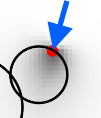
Figure 2: 2-D example of how part of the failure probability map looks after a collision. Here, the robot collided at the red dot with the unseen circle obstacle when moving in the direction of the blue arrow. The failure probability behind the collision is high, indicated by dark color, and in front of the collision low as indicated by a light color.

For estimating the probability of failure for a path, assuming independence of failures along the path, we would like to compute the geometric product integral over the failure probability density of the path. To approximate this, we discretize the path into $K$ segments and transform the joint configuration at each point along the discretized path into task space using forward kinematics. We then estimate path failure probability $p^{k}_{\textrm{FAIL}}$ for each point $k$ using Eq. 1 defined above and distance between consecutive points along the path (corresponds to rectangle rule in numerical product integration). We then estimate path failure $P(e=\textrm{FAIL}|p^{1\dots K}_{\textrm{FAIL}})$:

$$P(e=\textrm{FAIL}|p^{1\dots K}_{\textrm{FAIL}})=\prod_{k=1}^{K}p^{k}_{\textrm{FAIL}}=\exp\sum_{k=1}^{K}\log p^{k}_{\textrm{FAIL}},$$ (4)

where transforming the product into a sum of log terms can be important as part of a practical implementation to prevent underflow of floating point numbers.

IV Experiments

We performed experiments both in simulated randomly constructed 2-D and 3-D environments and with a 7-DOF KUKA LBR iiwa R820 robot arm. With the robot arm we disentangle an object from real plastic and iron waste and move the object out of a simple cardboard maze. We also disentangle a fluffy toy-bunny which is jammed in a cardboard box. In each run, we allow the robot to execute at most $20$ paths and measure the success rate. Success means arrival at the goal configuration $c_{\textrm{GOAL}}$. In the experiments, we have $K=100$, $\Delta=0.04$, $N_{\textrm{ITER}}=20$, $|C_{\textrm{RAND}}|=100$, $P_{\textrm{GOAL}}=0.1$, $d_{\textrm{DIST}}=0.04$, and no time limit.

IV-A Simulation

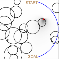
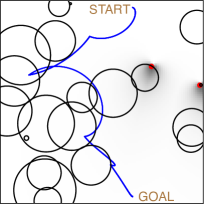
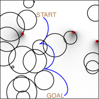
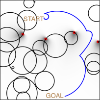
Figure 3: Visualization of a sequence of disentangling movements of a planar multi-link robot in 2-D simulation. At each time step the robot plans a path in joint space, shown by blue color in task space, to the goal configuration and tries to execute the path. Red dots show where the robot has previously collided with obstacles in task space. The robot does not observe the “real obstacles” shown as black circles but it can sense its current joint configuration. The robot’s probability map $\mathcal{M}$ for collisions is shown with dark-light colors. Dark color represents high collision probability and white color low collision probability. In this image sequence, the robot hits obstacles four times before finally arriving at the goal in the last image. As can be seen, the robot always tries to circumvent areas with high collision probability.

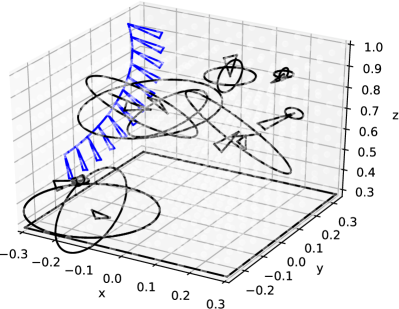
Figure 4: Visualization of 3-D disentangling simulation. Blue line depicts planned end-effector trajectory. Triangles show orientation of end-effector and obstacles. The robot does not observe the obstacles, only its joint configuration. Obstacles are either discs, depicted by circles, or balls, depicted by two orthogonal circles. Obstacle size varies. Obstacles can be circumvented by using an end-effector orientation dissimilar from the obstacle orientation. Making orientation in this way important is motivated by flexible objects which may allow you to pull the object and slide along the object with a suitable orientation. Note also that we evaluate the approaches with and without obstacle orientation.

In the experiments, the proposed algorithm always plans in 7 dimensional joint configuration space and checks for collisions in task space. In the simulations, we run experiments (1) in two dimensional task space where the end-effector is just a point mass at the end of a planar 7-DOF multi-link robot arm, (2) with a 3-D point mass at the end of a KUKA LBR 7-DOF robot arm, and (3) where the 3-D task space also includes the orientation of the end-effector. Case (1) is beneficial for visualizing the proposed approach. The real robot experiments use case (3). When checking for collisions or collision probability, in cases (1) and (2), the orientation of the end-effector is not taken into account, that is, $D_{\textrm{ORIENT}}(c,f)$ in Eq. 2 becomes zero. Fig. 3 shows a visualization of the 2-D simulation environment and Fig. 4 of the 3-D simulation environment.

The simulation experiments are designed to answer the following questions: (1) Does the robot learn to circumvent unknown obstacles and go to the goal position? (2) Is the robot able to plan paths through narrow spaces? We use environments with a varying number and size of obstacles. A large number of obstacles creates narrow spaces.

Our approach does not employ hard constraints. Since we do not know the exact shape or location of obstacles hard constraints could prevent the robot from going close to an obstacle, and, the robot would potentially not be able to solve some entanglements. We choose as comparison methods “Hard” and “Epsilon”. “Hard” is an RRT version which is identical to our proposed approach except that we use a probability threshold to make failure probabilities deterministic. This yields an algorithm called “Hard” similar to common hard constraint RRT approaches. “Hard” allows for a fair comparison to our proposed approach “Probabilistic” since the hard constraints have similar shape to the probability distributions used by “Probabilistic”. “Epsilon” is based on the epsilon-greedy strategy [37] widely used in reinforcement learning where the robot moves directly towards the goal with epsilon probability and otherwise in a random direction. We run different versions of these approaches with different hyper-parameter choices denoted by “Epsilon X”, where X denotes the epsilon value and “Hard Y” where Y denotes the probability threshold value. Fig. 5 shows the simulation results and Fig. 6 shows sensitivity analysis: “Probabilistic” outperforms the comparison methods in all environments and is not as sensitive to hyper-parameter choice.

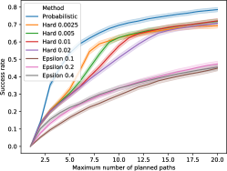
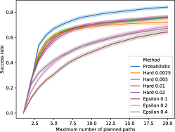
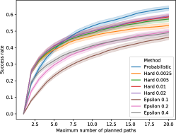
(a) 2-D	(b) 3-D	(c) 3-D with orientation

Figure 5: Evaluation in simulation. The results show for different maximum numbers of planned paths average success rate with a bootstrapped 95% confidence interval. We ran experiments for a varying number of obstacles. For each obstacle number we performed 100 random evaluations and report the total numbers. (a) Planar 2-D robot moving from initial joint configuration to goal configuration with 1, 10, 30, and 50 disc obstacles. (b) 3-D robot without taking orientation of the end-effector into account with 1, 10, 30, and 50 ball or disc obstacles. (c) 3-D robot taking orientation of the end-effector into account with 30, 50, 70, and 90 ball or disc obstacles. The proposed “Probabilistic” approach outperforms comparison methods.

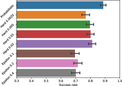
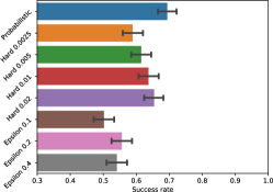
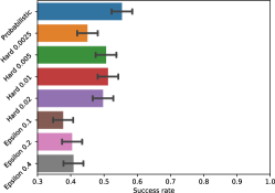
(a) 30 obstacles	(b) 50 obstacles	(c) 70 obstacles

Figure 6: Sensitivity analysis. For maximally $20$ planned paths in Fig. 5(c) we break down here the results according to the number of obstacles. While “Probabilistic” performs constantly well “Epsilon” and “Hard” are sensitive to the choice of hyper-parameter value. With 30 obstacles “Hard 0.02” performs better than “Hard 0.01” while with 70 obstacles “Hard 0.01” performs better than “Hard 0.02”. This makes intuitively sense since with more obstacles you have less space and do not want to block movements as much. With 30 obstacles “Epsilon 0.2” performs better than “Epsilon 0.4” while with 70 obstacles “Epsilon 0.4” performs better than “Epsilon 0.2”. An important thing to note is that in real robotic tasks the complexity or number and shape of obstacles is usually not known beforehand and thus hyper-parameter tuning is not feasible.

IV-B Robot experiments

In the robot experiments, the proposed algorithm plans in 7 dimensional joint configuration space. We used a 7-DOF KUKA LBR robot arm equipped with a SAKE gripper. The attached vision sensor shown in Fig. 1 and Fig. 7 was not used in the experiments. The robot experiments are designed to answer the following questions: (1) Can the proposed approach be used with a real robot? (2) Does the approach work in situations where the grasped object is flexible or the environment is flexible? (3) How does the proposed approach compare to the baselines in real robotic experiments?

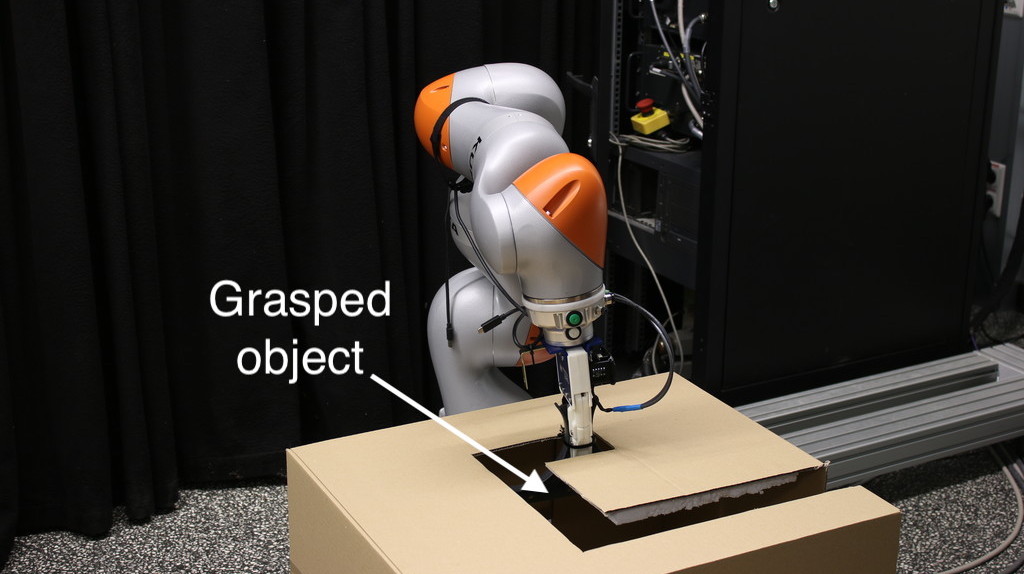
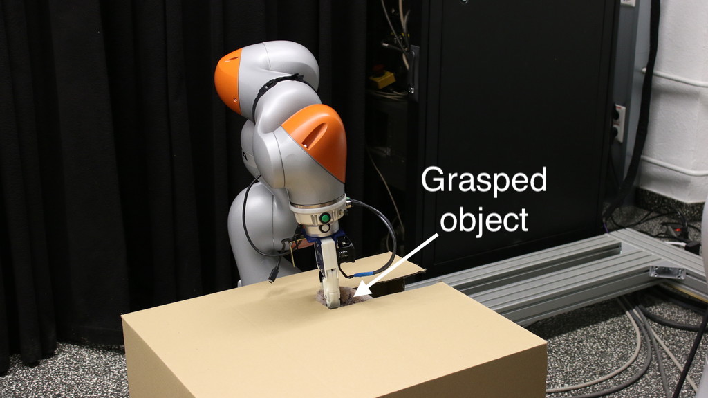
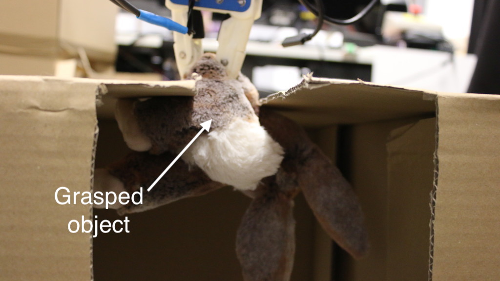
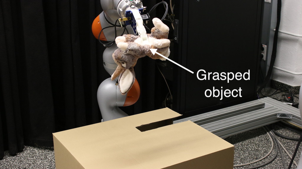
(a) Maze	(b) Bunny in a box	(c) Bunny in a box	(d) Bunny in a box

Figure 7: We have three robotic evaluation scenarios. (Waste) The waste evaluation scenario is shown in Fig. 1(top) where a grasped gray plastic object is entangled in plastic and iron waste and needs to be moved away from the waste. When moving the object up flexible waste is pulled up requiring a specific combination of movement and rotation of the end-effector. (Maze) Gray plastic object needs to be moved out of a simple maze. This can be accomplished by either rotating the object at a suitable location and pulling it up or by moving it through the maze and out of the side of the cardboard box. (Bunny) Bunny needs to be moved out of the box through the hole on the side of the cardboard box: (b) initial configuration, (c) side view highlighting the difficulty of the task, (d) successful final configuration. The robot does not use any sensors, does not know anything about the objects or the environment, and gets feedback only about its own position. Similarly to simulation experiments, in order to disentangle the end-effector the robot tries movement paths until succeeding or until 20 paths have been tried. In “Waste” the environment is flexible and in “Bunny” the grasped object is flexible.

TABLE I: How many times in ten evaluation runs each method succeeded to move the end-effector to the goal position in each robotic evaluation scenario shown in Figures 1 and 7.

Scenario	Epsilon	Hard	Probabilistic
Waste	6	3	7
Maze	4	0	6
Bunny	0	1	5
Total	10	4	18

Fig. 7 shows the three different real robot evaluation scenarios. We chose scenarios containing both flexible grasped and in-scene objects which are common in applications such as waste segregation. Table I shows performance in these scenarios. “Probabilistic” was best in all scenarios, especially in the “Bunny” experiment which we considered the hardest task a priori due to the constrained movements as shown in Fig. 7. “Epsilon” outperformed “Hard” in two out of three scenes which could be due to the hyper-parameter sensitivity shown in the simulations in Fig. 6. In successful runs, the average number of executed robot paths was $12.1$ for “Probabilistic”, $9.3$ for “Hard”, and $13.4$ for “Epsilon”. Planning a path, on a 4-core Intel i7 CPU, “Probabilistic” took from $9.9$ seconds ($|\mathcal{M}|=0$) to $17.4$ seconds (($|\mathcal{M}|=19$). “Hard” took from $9.7$ seconds to $17.7$ seconds. “Epsilon” took less than $0.2$ seconds for a planned path. Forward kinematics computation was most time-consuming. We used a Python implementation except we used C for forward kinematics. We expect speed ups with a full C-implementation and when using data structures such as KD-trees.

V Conclusion

When physically disentangling entangled objects we often do not have object models, and, especially with cluttered irregularly shaped objects, the robot can not create a model of the scene due to occlusion. Based on purely joint configuration information our approach learns a probability map of movement success and plans paths based on path success probability. The approach sequentially executes a planned path, incorporates information about movement success into the probability map and plans a new path. We demonstrate the approach successfully in simulated 2-D and 3-D environments and in three tasks with a real 7-DOF KUKA LBR robot arm while outperforming comparison methods. While the proposed approach worked well in the tasks we tried, we are currently working on a POMDP solution allowing more complex information gathering in even more complicated tasks. Due to our probabilistic formulation incorporating prior knowledge from sensors should be straightforward in future work. To speed up the replanning part of our approach further, we could combine ideas from [38, 39, 40]. In particular, we could use caching together with discarding parts of the RRT tree that are sub-optimal according to an admissible heuristic while updating collision probabilities of existing RRT edges and nodes. Finally, another possible direction for future work would be to adapt our approach to new disassembly applications in recycling.

References

- [1] A. Wade. (2015) Sellafield plutonium a multi-layered problem.
- [2] F. Pearce. (2015) Shocking state of world’s riskiest nuclear waste site.
- [3] National Audit Office, Progress on the Sellafield site: an update, 2015.
- [4] S. M. LaValle and J. J. Kuffner Jr, “Randomized kinodynamic planning,” The International Journal of Robotics Research, vol. 20, no. 5, pp. 378–400, 2001.
- [5] L. Kavraki, P. Svestka, J.-C. Latombe, and M. Overmars, “Probabilistic roadmaps for path planning in high-dimensional configuration spaces,” IEEE Transactions on Robotics and Automation, vol. 12, no. 4, pp. 566–580, 1996.
- [6] S. M. LaValle, Planning algorithms. Cambridge University Press, 2006.
- [7] S. Karaman and E. Frazzoli, “Incremental sampling-based algorithms for optimal motion planning,” in Robotics: Science and Systems (R:SS) conference, 2006.
- [8] Y. Yang and O. Brock, “Elastic roadmaps—motion generation for autonomous mobile manipulation,” Autonomous Robots, vol. 28, no. 1, p. 113, 2010.
- [9] S. S. Ge and Y. J. Cui, “New potential functions for mobile robot path planning,” IEEE Transactions on Robotics and Automation, vol. 16, no. 5, pp. 615–620, 2000.
- [10] Y. Hu and S. X. Yang, “A knowledge based genetic algorithm for path planning of a mobile robot,” in IEEE International Conference on Robotics and Automation, vol. 5. IEEE, 2004, pp. 4350–4355.
- [11] V. J. Lumelsky and A. A. Stepanov, “Path-planning strategies for a point mobile automaton moving amidst unknown obstacles of arbitrary shape,” Algorithmica, vol. 2, no. 1, pp. 403–430, 1987.
- [12] A. Stentz, “Optimal and efficient path planning for partially-known environments,” in IEEE International Conference on Robotics and Automation (ICRA), vol. 94, 1994, pp. 3310–3317.
- [13] P. E. Hart, N. J. Nilsson, and B. Raphael, “A formal basis for the heuristic determination of minimum cost paths,” IEEE Transactions on Systems Science and Cybernetics, vol. 4, no. 2, pp. 100–107, 1968.
- [14] J. Van Den Berg, D. Ferguson, and J. Kuffner, “Anytime path planning and replanning in dynamic environments,” in IEEE International Conference on Robotics and Automation (ICRA). IEEE, 2006, pp. 2366–2371.
- [15] M. Hoy, A. S. Matveev, and A. V. Savkin, “Algorithms for collision-free navigation of mobile robots in complex cluttered environments: a survey,” Robotica, vol. 33, no. 3, pp. 463–497, 2015.
- [16] J. A. Tobaruela and A. O. Rodríguez, “Reactive navigation in extremely dense and highly intricate environments,” PloS one, vol. 12, no. 12, 2017.
- [17] M. Wang et al., “Fuzzy logic based robot path planning in unknown environment,” in Proceedings of International Conference on Machine Learning and Cybernetics, vol. 2. IEEE, 2005, pp. 813–818.
- [18] L. Lei, H. Wang, and Q. Wu, “Improved genetic algorithms based path planning of mobile robot under dynamic unknown environment,” in IEEE International Conference on Mechatronics and Automation. IEEE, 2006, pp. 1728–1732.
- [19] J. Sfeir, M. Saad, and H. Saliah-Hassane, “An improved artificial potential field approach to real-time mobile robot path planning in an unknown environment,” in IEEE International Symposium on Robotic and Sensors Environments (ROSE). IEEE, 2011, pp. 208–213.
- [20] Y. K. Hwang and N. Ahuja, “A potential field approach to path planning,” IEEE Transactions on Robotics and Automation, vol. 8, no. 1, pp. 23–32, 1992.
- [21] O. Montiel, U. Orozco-Rosas, and R. Sepúlveda, “Path planning for mobile robots using bacterial potential field for avoiding static and dynamic obstacles,” Expert Systems with Applications, vol. 42, no. 12, pp. 5177–5191, 2015.
- [22] J. Mainprice and D. Berenson, “Human-robot collaborative manipulation planning using early prediction of human motion,” in IEEE/RSJ International Conference on Intelligent Robots and Systems (IROS). IEEE, 2013, pp. 299–306.
- [23] J. Cortés, L. Jaillet, and T. Siméon, “Disassembly path planning for complex articulated objects,” IEEE Transactions on Robotics, vol. 24, no. 2, pp. 475–481, 2008.
- [24] T. J. Lukka, T. Tossavainen, J. V. Kujala, and T. Raiko, “Zenrobotics recycler–robotic sorting using machine learning,” in International Conference on Sensor-Based Sorting (SBS), 2014.
- [25] J. V. Kujala, T. J. Lukka, and H. Holopainen, “Classifying and sorting cluttered piles of unknown objects with robots: a learning approach,” in IEEE/RSJ International Conference on Intelligent Robots and Systems (IROS). IEEE, 2016, pp. 971–978.
- [26] S. G. Paulraj, S. Hait, and A. Thakur, “Automated municipal solid waste sorting for recycling using a mobile manipulator,” in International Design Engineering Technical Conferences and Computers and Information in Engineering Conference. ASME, 2016.
- [27] S. P. Gundupalli, S. Hait, and A. Thakur, “A review on automated sorting of source-separated municipal solid waste for recycling,” Waste management, vol. 60, pp. 56–74, 2017.
- [28] A. Saxena, J. Driemeyer, and A. Y. Ng, “Robotic grasping of novel objects using vision,” The International Journal of Robotics Research, vol. 27, no. 2, pp. 157–173, 2008.
- [29] J. Maitin-Shepard, M. Cusumano-Towner, J. Lei, and P. Abbeel, “Cloth grasp point detection based on multiple-view geometric cues with application to robotic towel folding,” in IEEE International Conference on Robotics and Automation (ICRA). IEEE, 2010, pp. 2308–2315.
- [30] I. Lenz, H. Lee, and A. Saxena, “Deep learning for detecting robotic grasps,” The International Journal of Robotics Research, vol. 34, no. 4-5, pp. 705–724, 2015.
- [31] K. J. Åström, “Optimal control of Markov processes with incomplete state information,” Journal of Mathematical Analysis and Applications, vol. 10, no. 1, pp. 174–205, 1965.
- [32] L. Kaelbling, M. Littman, and A. Cassandra, “Planning and acting in partially observable stochastic domains,” Artificial intelligence, vol. 101, no. 1, pp. 99–134, 1998.
- [33] C. H. Papadimitriou and J. N. Tsitsiklis, “The complexity of Markov decision processes,” Mathematics of operations research, pp. 441–450, 1987.
- [34] J. J. Kuffner and S. M. LaValle, “RRT-connect: An efficient approach to single-query path planning,” in IEEE International Conference on Robotics and Automation (ICRA), vol. 2. IEEE, 2000, pp. 995–1001.
- [35] S. Klemm, J. Oberländer, A. Hermann, A. Roennau, T. Schamm, J. M. Zollner, and R. Dillmann, “RRT∗-Connect: Faster, asymptotically optimal motion planning,” in IEEE International Conference on Robotics and Biomimetics (ROBIO). IEEE, 2015, pp. 1670–1677.
- [36] D. Q. Huynh, “Metrics for 3d rotations: Comparison and analysis,” Journal of Mathematical Imaging and Vision, vol. 35, no. 2, pp. 155–164, 2009.
- [37] R. S. Sutton and A. G. Barto, Reinforcement learning: An introduction. MIT press, 2018.
- [38] J. Bruce and M. M. Veloso, “Real-time randomized path planning for robot navigation,” in Robot Soccer World Cup. Springer, 2002, pp. 288–295.
- [39] D. Ferguson and A. Stentz, “Anytime RRTs,” in IEEE/RSJ International Conference on Intelligent Robots and Systems (IROS). IEEE, 2006, pp. 5369–5375.
- [40] D. Ferguson, N. Kalra, and A. Stentz, “Replanning with RRTs,” in IEEE International Conference on Robotics and Automation (ICRA). IEEE, 2006, pp. 1243–1248.