Neutral compact spherically symmetric stars in teleparallel gravity

Abstract

We present novel neutral and uncharged solutions that describe the cluster of Einstein in the teleparallel equivalent of general relativity (TEGR). To this end, we use a tetrad field with non-diagonal spherical symmetry which gives the vanishing of the off-diagonal components for the gravitational field equations in the TEGR theory. The clusters are calculated by using an anisotropic energy-momentum tensor. We solve the field equations of TEGR theory, using two assumptions: the first one is by using an equation of state that relates density with tangential pressure while the second postulate is to assume a specific form of one of the two unknown functions that appear in the non-diagonal tetrad field. Among many things presented in this study, we investigate the static stability specification. We also study the Tolman-Oppenheimer-Volkoff equation of these solutions in addition to the conditions of energy. The causality constraints with the adiabatic index in terms of the limit of stability are discussed.

I Introduction

To investigate the importance of astrophysics or astronomy with gravitational waves, the theory of General Relativity (GR) plays an essential role in astrophysical systems like compact objects and radiation with high energy usually from strong gravity field around neutron stars and black holes Shekh and Chirde (2019).

Recently, observations show that our universe is experiencing cosmic acceleration. The existence of a peculiar energy component called dark energy (DE) controlling the universe is guaranteed by many observations including type Ia supernovae (SNeIa), the Wilkinson Microwave Anisotropy Probe (WMAP) and the Planck in terms of the cosmic microwave background (CMB) radiation, the surveys of the large-scale structure (LSS) Perlmutter et al. (1999); Spergel et al. (2007); Hawkins et al. (2003); Eisenstein et al. (2005); Aghanim et al. (2018). In terms of an equation of state for dark energy, $p=\omega\rho$, when $\omega<-1/3$ the accelerated expansion is realized, when $-1/3<\omega<-1$ we have quintessence regime, when $\omega<-1$ we have a phantom regime, and when $p=-\rho$ we have a gravastar (gravitational vacuum condensate star) Mazur and Mottola (2001, 2004); Usmani et al. (2011); Rahaman et al. (2012a, b); Bhar (2014); Yousaf et al. (2019). Explanations for the properties of DE have been proposed; among those are: 1) Modifications of the cosmic energy by involving novel components of DE like a scalar field including quintessence Copeland et al. (2006); Papantonopoulos (2007). 2) Modifications of GR action to derive different kinds of amendment theories of gravity like $f(T)$ gravity Bengochea and Ferraro (2009); Cai et al. (2016); Bamba et al. (2012); Saha and Debnath (2018), where $T$ is the torsion scalar in teleparallelism; $f(R)$ gravity De Felice and Tsujikawa (2010); Nojiri and Odintsov (2011); Capozziello and De Laurentis (2011); Nojiri et al. (2017); Faraoni and Capozziello (2011); Bamba and Odintsov (2015); Ruiz-Lapuente (2010) with $R$ the scalar curvature; $f(G)$ gravity with $G$ the Gauss-Bonnet invariant Cognola et al. (2006); $f(R,{\cal T})$ gravity, where ${\cal T}$ the trace of the energy-momentum tensor of matter Harko et al. (2011), etc. Teleparallel equivalent of general relativity (TEGR) is another formulation of GR whose dynamical variables are the tetrad fields defined as ${l^{i}}_{\mu}$. Here, at each point $x^{\mu}$ on a manifold, $i$ is the orthonormal basis of the tangent space, and $\mu$ denotes the coordinate basis and both of the indices run from $0\cdots 3$. In Einstein’s GR the torsion is absent and the gravitational field is described by curvature while in TEGR theory, the curvature is vanishing identically and the gravitational field is described by torsion ARCOS and PEREIRA (2004); Sotiriou et al. (2011); Camera and Nishizawa (2013); Aldrovandi and Pereira (2013); Sahlu et al. (2019); Horvat et al. (2015); Liddle et al. (1994). Fortunately, the two theories describe the gravitational field equivalently on the background of the Lagrangian up to a total divergence term Nashed (2008, 2019).

The Einstein’s cluster Einstein (1939) was presented in the literature at the beginning of the last century to discuss stationary gravitating particles, each of which move in a circular track around the center for them in the influence of the effect from the gravity field. When such particles rotate on the common track and have the same phases, they constitute a shell that is named “Einstein’s Shell”. The construction layers for the Einstein’s shell form the Einstein’s Cluster. The distribution of such a particle has spherical symmetry and it is continuous and random. These particles have the collision-less geodesics. When the gravitational field is balanced by the centrifugal force the above systems are called static and are in equilibrium. A thick matter shell with the spherical symmetry is constituted by the procedure described above. The resultant configuration has no radial pressure and there exists only its stress in the tangential direction. There are many studies of the Einstein clusters in the literature Florides (1974); Zapolsky (1968); Gilhert (1954); Comer and Katz (1993). For the spherically symmetric case the energy-momentum tensor has anisotropic form, i.e. ${T^{0}}_{0}=-\rho$, ${T^{r}}_{r}=p_{r}$, and ${T^{\theta}}_{\theta}={T^{\phi}}_{\phi}=p_{t}$, where ${T^{\mu}}_{\nu}$ is the matter energy-momentum tensor, $\rho$ is the energy density, $p_{r}$ and $p_{t}$ are the radial and tangential pressures, respectively. By using the junction condition it can be found that the pressure in the radial direction vanishes for the Einstein’s clusters. Recently, the compact objects filled with fluids with their anisotropy have been attracted and their structure and evolutional processes have been studied Mak and Harko (2003); Chaisi and Maharaj (2005); Herrera et al. (2004); Abreu et al. (2007); Thirukkanesh and Maharaj (2008); Maurya et al. (2015); Folomeev and Dzhunushaliev (2015); Kalam et al. (2012); Maurya et al. (2019); Bhar et al. (2017, 2016); Singh et al. (2017); Böhmer and Harko (2006); Andréasson and Böhmer (2009). It is the aim of this study to apply a non-diagonal tetrad field that possesses spherical symmetry to the non-vacuum equation of motions of TEGR theory and try to derive novel solutions and discuss their physical contents.

The arrangements of this paper are the followings. In Sec. II we explain the basic formulae in terms of TEGR. In Sec. III the gravitational field equations for the TEGR theory in the non-vacuum background are applied to a non-diagonal tetrad and the non-zero components in terms of these differential equations are derived. The number of the differential equations with their non-linearity is found to be less than the number of unknowns. Therefore, we postulate two different assumptions and derive two novel solutions in this section. In Sec. IV we discuss the physical contents of these two solutions and show that the second solution possesses many merits that make it physically acceptable. Among these things that make the second solution physically acceptable is that it satisfies the energy conditions, the TOV equation is satisfied, it has static stability and its adiabatic index is satisfied. In Sec. V discussions and conclusions of the present considerations are given.

II Basic Formulae of Teleparallel Equivalent of General Relativity (TEGR)

In this section we describe the basic formulae of TEGR. The tetrad field ${l^{i}}_{\mu}$, covariant, and its inverse one $l_{i}{}^{\mu}$, contravariant, play a role of the fundamental variables for TEGR. These quantities satisfy the following relation

$$\bm{l_{\nu}}=l^{i}{}_{\nu}\bm{l_{i}},\qquad\bm{l_{i}}=l_{i}{}^{\nu}\bm{l_{\nu}}.$$ (1)

Based on the tetrads the metric tensor is defined by

$$g_{{}_{{}_{\beta\alpha}}}=\eta_{ij}l^{i}{}_{\mu}l^{j}{}_{\nu}=\vec{l}_{\mu}\cdot\vec{l}_{\nu}\,.$$ (2)

Here $\eta_{ab}$ denotes the Minkowski spacetime and it is given by $\eta_{ab}=diag(-1,+1,+1,+1)$. Moreover, $\vec{l}_{\mu}$ is the co-frame.

Using the above equations one can easily prove the following identities:

$$\eta_{ij} =g_{\mu\nu}l_{i}{}^{\mu}l_{j}{}^{\nu}=\vec{l}_{i}\cdot\vec{l}_{j}, \eta^{ij} =g^{\mu\nu}l^{i}{}_{\mu}l^{j}{}_{\nu},$$ (3a)

$$g^{\mu\nu} =\eta^{ij}l_{i}{}^{\mu}l_{j}^{\nu}, l =\sqrt{|g|},$$ (3b)

$$l^{i}{}_{\mu}l_{i}{}^{\nu} =\delta^{\nu}_{\mu}, l^{i}{}_{\mu}l_{j}{}^{\mu} =\delta^{i}_{j}\,.$$ (3c)

With the spin connection the curvature quantity and the trosion one can be written as

$$R^{ij}{}_{\mu\nu} := \partial_{\mu}\omega^{ij}{}_{\nu}-\partial_{\nu}\omega^{ij}{}_{\mu}+\omega^{i}{}_{s\mu}\omega^{sj}{}_{\nu}-\omega^{i}{}_{s\nu}\omega^{sj}{}_{\mu}\,,$$ (4)

$$T^{i}{}_{\mu\nu} := \partial_{\mu}l^{i}{}_{\nu}-\partial_{\nu}b^{i}{}_{\mu}+\omega^{i}{}_{k\mu}l^{k}{}_{\nu}-\omega^{i}{}_{k\nu}l^{k}{}_{\mu},$$ (5)

where $\omega^{ij}{}_{\nu}$ is the spin connection. The matrices with the local Lorentz symmetry, $\Lambda^{a}{}_{b}$, generates the spin connection as

$$\omega^{a}{}_{b\mu}=\omega^{a}{}_{b\mu}(\Lambda)=\Lambda^{a}{}_{c}\partial_{\mu}(\Lambda^{-1})^{c}{}_{b},\quad\eta_{ab}\Lambda^{a}{}_{c}\Lambda^{b}{}_{d}=\eta_{cd}\,.$$ (6)

The tensors $R^{\mu}{}_{\nu\rho\sigma}$ and $T^{i}{}_{\mu\nu}$ are defined as follows:

1. $R^{\mu}{}_{\nu\rho\sigma}=l_{i}{}^{\mu}l_{j\nu}R^{ij}{}_{\rho\sigma},$

2. $l^{i}{}_{\sigma}T^{\sigma}{}_{\mu\nu}=T^{i}{}_{\mu\nu}\;.$

Using the above data one can define the torsion in terms of the derivative of tetrad and spin connection as

$$T^{a}{}_{\mu\nu}=2\left(\partial_{[\mu}l^{a}{}_{\nu]}+\omega^{a}{}_{b[\mu}l^{b}{}_{\nu]}\right)\,,$$ (7)

where square brackets denote that the pair of indices are skew-symmetric and $\partial_{\mu}=\frac{\partial}{\partial x^{\mu}}$. In the TEGR theory, the spin connection is set to be zero ($\omega^{a}{}_{b\mu}=0$). Therefore, the torsion tensor takes the form

$$T^{a}{}_{\mu\nu}=\partial_{[\mu}l^{a}{}_{\nu]}.$$

The TEGR theory is constructed by using the Lagrangian

$$L_{\rm TEGR}=\int\mathrm{d}^{4}x\ |l|\left(\frac{1}{2\kappa^{2}}T+\mathcal{L}_{\rm m}(g,\Psi)\right)\,,$$ (8)

with $\kappa^{2}=8\pi$. Here $\mathcal{L}_{\rm m}(g,\Psi)$ is the Lagrangian of matter with minimal coupling to gravitation through the metric tensor written with the tetrad fields. In addition, $T$ is the torsion scalar and it is defined as

$$T=T^{a}{}_{\mu\nu}S_{a}{}^{\mu\nu}=\frac{1}{2}\left(l_{a}{}^{\sigma}g^{\rho\mu}l_{b}{}^{\nu}+2l_{b}{}^{\rho}g^{\sigma\mu}l_{a}{}^{\nu}+\frac{1}{2}\eta_{ab}g^{\mu\rho}g^{\nu\sigma}\right)T^{a}{}_{\mu\nu}T^{b}{}_{\rho\sigma}\,.$$ (9)

The superpotential $S_{a}{}^{\mu\nu}$ is defined as

$$S_{a}{}^{\mu\nu}=\frac{1}{2}(K^{\mu\nu}{}_{a}-h_{a}{}^{\mu}T_{\lambda}{}^{\lambda\nu}+h_{a}{}^{\nu}T_{\lambda}{}^{\lambda\mu}),$$

with $K^{\mu\nu}{}_{a}$ the contortion tensor, expressed by

$$K^{\mu\nu}{}_{a}=\frac{1}{2}(T^{\nu\mu}{}_{a}+T_{a}{}^{\mu\nu}-T^{\mu\nu}{}_{a})\,.$$

Variation of the Lagrangian (8) with respect to a tetrad $l^{a}{}_{\mu}$ yields Maluf et al. (2002); Nashed (2011)

$$\frac{1}{4}Tl_{a}{}^{\mu}+T^{b}{}_{\nu a}S_{b}{}^{\mu\nu}+\frac{1}{l}\partial_{\nu}(lS_{a}{}^{\mu\nu}) =\frac{1}{2}\kappa^{2}\Theta_{a}{}^{\mu}\,.$$ (10)

The stress-energy tensor, $\Theta_{a}{}^{\mu}$, is the energy-momentum tensor for fluids whose configuration has anisotropy and it is represented by

$$\Theta_{a}{}^{\mu}{}=(p_{t}+\rho)u^{\mu}u_{a}+p_{t}\delta_{a}{}^{\mu}+(p_{r}-p_{t})\xi_{a}\xi^{\mu}\,,$$ (11)

with $u_{\mu}$ the time-like vector defined as $u^{\mu}=[1,0,0,0]$ and $\xi_{\mu}$ the unit radial vector with its space-like property, defined by $\xi^{\mu}=[0,1,0,0]$ such that $u^{\mu}u_{\mu}=-1$ and $\xi^{\mu}\xi_{\mu}=1$. Here $\rho$ means the energy density, $p_{r}$ and $p_{t}$ are the radial and tangential pressures, respectively.

III Neutral compact stars

In this section we adopt the gravitational field equation (10) to the tetrad with its spherical symmetry, which represents a dense compact relativistic star.

Based on the spherical coordinates $(t,r,\theta,\phi)$, the metric with its spherical symmetry is given by

$$ds^{2}=-e^{\mu(r)}\,dt^{2}+e^{\nu(r)}dr^{2}+r^{2}d\Omega^{2}\;,\quad\quad d\Omega^{2}=(d\theta^{2}+\sin^{2}\theta d\phi^{2})\,,$$ (12)

where $\mu(r)$ and $\nu(r)$ are the functions of $r$ in the radial direction. This line element in Eq. (12) can be reproduced from the following tetrad field  Bahamonde et al. (2019):

$$l^{a}{}_{\mu}=\left(\begin{array}[]{cccc}e^{\mu(r)/2}&0&0&0\\ 0&e^{\nu(r)/2}\cos(\phi)\sin(\theta)&r\cos(\phi)\cos(\theta)&-r\sin(\phi)\sin(\theta)\\ 0&e^{\nu(r)/2}\sin(\phi)\sin(\theta)&r\sin(\phi)\cos(\theta)&r\cos(\phi)\sin(\theta)\\ 0&e^{\nu(r)/2}\cos(\theta)&-r\sin(\theta)&0\\ \end{array}\right)\,.$$ (13)

We mention that the tetrad (13) is an output product of a diagonal tetrad and local Lorentz transformation, i.e., one can write it as

$$l^{a}{}_{\mu}=\Lambda^{a}{}_{b}l^{b}{}_{\mu_{diag}}$$

$$\Rightarrow\left(\begin{array}[]{cccc}e^{\mu(r)/2}&0&0&0\\ 0&e^{\nu(r)/2}\cos(\phi)\sin(\theta)&r\cos(\phi)\cos(\theta)&-r\sin(\phi)\sin(\theta)\\ 0&e^{\nu(r)/2}\sin(\phi)\sin(\theta)&r\sin(\phi)\cos(\theta)&r\cos(\phi)\sin(\theta)\\ 0&e^{\nu(r)/2}\cos(\theta)&-r\sin(\theta)&0\\ \end{array}\right)$$ (18)

$$\equiv\left(\begin{array}[]{cccc}1&0&0&0\\ 0&\cos(\phi)\sin(\theta)&\cos(\phi)\cos(\theta)&-\sin(\phi)\\ 0&\sin(\phi)\sin(\theta)&\sin(\phi)\cos(\theta)&\cos(\phi)\\ 0&\cos(\theta)&-\sin(\theta)&0\\ \end{array}\right)\times\left(\begin{array}[]{cccc}e^{\mu(r)/2}&0&0&0\\ 0&e^{\nu(r)/2}&0&0\\ 0&0&r&0\\ 0&0&0&r\sin(\theta)\\ \end{array}\right)\,.$$ (27)

Using Eq. (13) in Eq. (9) the torsion scalar takes the form

$$T=\frac{2e^{-\nu}\left[e^{\nu}-e^{\nu/2}(2+r\mu^{\prime})+1+r\mu^{\prime}\right]}{r^{2}}\,.$$ (28)

It follows from Eq. (28) that $T$ vanishes in the limit $\mu=\nu\rightarrow 0$ unlike what has been studied before in the literature Bahamonde et al. (2019). Using Eq. (28) in the field equations (10) we get

$$8\pi\rho = -\frac{1-e^{-\nu}(1-r\nu^{\prime})}{r^{2}}\,,$$

$$8\pi p_{r} = \frac{e^{-\nu}(1-r\mu^{\prime})-1}{r^{2}}\,,$$

$$8\pi p_{t} = -\frac{e^{-\nu}\left[2r\mu^{\prime\prime}+(r\mu^{\prime}+2)(\mu^{\prime}-\nu^{\prime})\right]}{4r}\,,$$ (29)

where ^′ denotes derivatives with respect to $r$. These differential equations are three independent equations in five unknowns: $\mu$, $\nu$ and $\rho$, $p_{r}$ and $p_{t}$. Therefore, we need extra conditions to be able to solve the above system. The extra conditions are the zero radial pressure, namely, $p_{r}=0$ Boehmer and Harko (2007); Singh et al. (2019), and assuming the equation of state (EoS) in terms of the energy density and the tangential pressure. We can represent these conditions as

$$p_{r}=0,\qquad\qquad p_{t}=\omega_{t}\rho\,,$$ (30)

where $\omega_{t}$ is the EoS parameter for anisotropic fluids.

Substituting Eq. (30) into (29) we obtain

$$\rho=\frac{\omega_{t}}{2\pi r^{2}(1+4\omega_{t})},\qquad\mu=4\omega_{t}\ln(r)+c_{1},\qquad\nu=\ln(4\omega_{t}+1),\qquad p_{t}=\omega_{t}\rho\,,$$

$$\rho=0,\qquad\mu=\ln\Big{(}\frac{c_{3}r-c_{2}}{r}\Big{)},\qquad\nu=\ln\Big{(}\frac{rc_{3}}{c_{3}r-c_{2}}\Big{)},\qquad p_{t}=0\,.$$ (31)

We note that the vanishing of the reason why the tangential pressure as well as the energy density vanish as in the second set of Eq. (III) is due to the composition of the two unknown functions $\mu$ and $\nu$ that give the Schwarzschild solution.

Another solution that can be derived from Eq. (29) is through the assumption of the unknown function $\mu$ to have the form Singh et al. (2019)

$$\mu(r)=\ln(b_{0}+b_{1}r^{2}+b_{2}r^{4})\;.$$ (32)

Using Eq. (32) in (29) we get the remaining unknown functions in the form

$$\rho=\frac{(3b_{1}+10b_{2}r^{2})(b_{0}+b_{1}r^{2}+b_{2}r^{4})}{4\pi(b_{0}+3b_{1}r^{2}+5b_{2}r^{4})^{2}},\qquad\qquad\qquad\nu=\ln\Big{(}\frac{b_{0}+3b_{1}r^{2}+5b_{2}r^{4}}{b_{0}+b_{1}r^{2}+b_{2}r^{4}}\Big{)}\,,$$

$$p_{t}=\frac{r^{2}(3b_{1}[b_{1}+16b_{2}r^{2}]+20b_{2}{}^{2}r^{4})}{8\pi(b_{0}+3b_{1}r^{2}+5b_{2}r^{4})^{2}}\;.$$ (33)

The EoS of the first and second solutions given by Eqs. (III) and (III) takes the form

$$\omega_{t_{1}}=1\,,\qquad\qquad\omega_{t_{2}}=\frac{r^{2}(b_{1}+2b_{2}r^{2})}{2(b_{0}+b_{1}r^{2}+b_{2}r^{4})}\,.$$ (34)

The first EoS shows that we have a stiff matter while the behavior of the second EoS is shown in Fig. 21(c) below.

The behavior of the density and tangential pressure of the first and second solutions are drawn in Fig. 1. Figs. 11(a) 11(b) show that energy and pressure decrease as the radial coordinate $r$ increases. For the second solution, Figs. 21(a), 21(b) and 21(c) show that the energy density and pressure become the maximum values for $r=1.5\leavevmode\nobreak\ \mathrm{km}\sim 0.2\leavevmode\nobreak\ \mathrm{km}$ depending on the free parameter $b_{0}$ and then decreasing. As for the EoS parameter of the second solution it takes negative values and then positive values depending also on the value of the free parameter $b_{0}$. The reason for the variation of the EoS from $negative$ value to $positive$ is because the dominator of Eq. (34) has only two real solutions that have the form

$$\pm\frac{\sqrt{\sqrt{b_{1}{}^{2}-4b_{0}b_{2}}-b_{1}}}{\sqrt{2b_{2}}},\qquad\qquad b_{2}>0.$$ (35)

Equation (35) ensures that the parameter $b_{2}$ must not have a zero value and $b_{0}<0$ which are consistent with the values given in Fig.21(c) and through the whole of the present study.

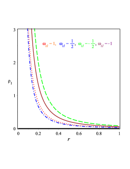
(a)  Density of the first solution

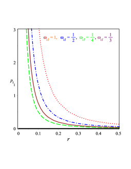
(b)  Pressure of the first solution

Figure 1: Schematic plot of the radial coordinate $r$ in the unit of km versus the energy density and pressure of the solution (III).

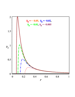
(a)  Density of the second solution

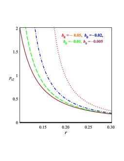
(b)  Pressure of the second solution

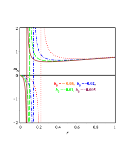
(c)  EoS of the second solution

Figure 2: Schematic plot of the radial coordinate $r$ in the unit of km versus the energy density, pressure and the EoS of the solution (III) when $b_{1}=b_{2}=1$.

We consider the physical contents for the first and second solutions. To this end, we are going to calculate the following quantities. The surface red-shift of the first and second solutions takes the form:

$$z_{s_{1}}=e^{\nu_{s}}-1=4\omega_{t_{1}}\;,\qquad\qquad z_{s_{2}}=\frac{2r^{2}(b_{1}+2b_{2}r^{2})}{b_{0}+b_{1}r^{2}+b_{2}r^{4}}\;.$$ (36)

The behavior of the surface red-shift of the second solution is identical with the behavior of the EoS, as shown in Fig. 21(c), because the two forms are identical up to some constant. The gravitational mass of a spherically symmetric source with the radial dependence $r$ is expressed by Singh et al. (2019)

$$m(r)=4\pi{\int_{0}}^{r}\rho(\xi)\xi^{2}d\xi\;,$$ (37)

which gives for solutions (III) and (III) the form

$$m_{1}(r)=\frac{2\omega_{t_{1}}r}{4\omega_{t{1}}+1}\,,\qquad\qquad m_{2}(r)=\frac{20b_{2}r^{3}(b_{1}+2b_{2}r^{2})}{(3b_{1}+10b_{2}r^{2})^{2}-9b_{1}{}^{2}+20b_{0}b_{2}}\;.$$ (38)

The behavior of the gravitational mass of solutions (III) and (III) are drawn in Fig. 32(a) and 32(b). This figures show the gravitational mass increases with the radial coordinate. The compactness parameter of a source with its spherical symmetry in terms of the radius $r$ takes the form Singh et al. (2019)

$$u(r)=\frac{2m(r)}{r}\,,\qquad\qquad\textrm{that\, gives\, for\, solutions\, (\ref{sol})\, and\, (\ref{sol1})\, the\, form}$$

$$u_{1}(r)=\frac{4\omega_{t_{1}}}{4\omega_{t_{1}}+1}\,,\qquad\qquad u_{2}(r)=\frac{20r^{2}(b_{1}+2b_{2}r^{2})}{(3b_{0}+10b_{2}r^{2})^{2}-9a1^{2}+20b_{0}b_{2}}.$$ (39)

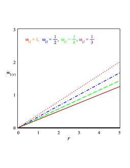
(a)  Mass of solution (III) against radial coordinate

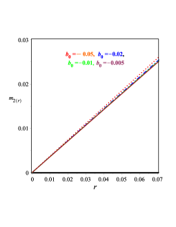
(b)  Mass of solution (III) against radial coordinate

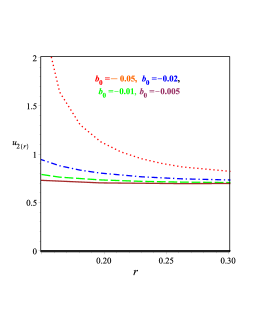
(c)  Compactness parameter of solution (III) against radial coordinate

Figure 3: Schematic plot of the gravitational mass of solutions (III) and (III) and compactness parameter versus the radial coordinate $r$ in km when $b_{1}=b_{2}=1$.

We show the behavior of compactness parameter of solution (III), because solution (III) gives a constant value, in Fig. 32(c) which shows some kind of inverse relation, i.e., when $r$ increase $u$ decreases.

The gradient of density and pressure of (III) and (III) take the form Singh et al. (2019)

$$d\rho_{1}=-\frac{\omega_{t}}{2\pi r^{3}(1+4\omega_{t})}\,,\qquad\qquad\qquad dp_{{t_{1}}}=-\frac{\omega^{2}_{t}}{2\pi r^{3}(1+4\omega_{t})}\,,$$

$$d\rho_{2}=-\frac{r(10b_{0}^{2}b_{2}-8b_{0}b_{2}r^{2}[8b_{1}+15b_{2}r^{2}]-5b_{1}b_{2}r^{4}[9b_{1}+20b_{2}r^{2}]-15b_{0}b_{2}^{2}-r^{2}[9b_{1}^{3}+50b_{2}^{3}r^{6}])}{2\pi(b_{0}+3b_{1}r^{2}+5b_{2}r^{4})^{3}}\,,$$

$$dp_{{t_{2}}}=\frac{r(3b_{0}[b_{1}^{2}+20b_{2}^{2}r^{4}]-9b_{1}^{2}r^{2}[b_{1}+5b_{2}r^{2}]-100b_{2}{}^{2}r^{6}[b_{1}+b_{2}r^{2}]+32b_{0}b_{1}b_{2}r^{2})}{4\pi(b_{0}+3b_{1}r^{2}+5b_{2}r^{4})^{3}}\,.$$

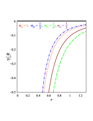
(a)  Variation of density (III) against radial coordinate

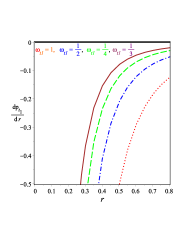
(b)  Variation of pressure (III) against radial coordinate

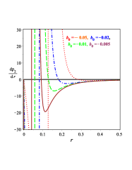
(c)  Variation of density (III) against radial coordinate

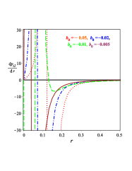
(d)  Variation of pressure (III) against radial coordinate

Figure 4: Variation of the gradient of density and pressure of (III) and (III) against $r$ in km when $b_{1}=b_{2}=1$.

Figure 4 shows that for solution (III) we have always negative gradient for density and pressure while for solution (III) we have negative value of the gradient of density then this negative changes to positive value and then become negative forever. The change of the sign of density occurs because the dominator of Eq. (III), i.e., $(b_{0}+3b_{1}r^{2}+5b_{2}r^{4})$ has two real solutions $\pm\frac{\sqrt{b_{2}(\sqrt{9b_{1}{}^{2}-20b_{0}b_{2}}-3b_{1})}}{\sqrt{10b_{2}}}$ which again ensure that the parameter $b_{2}\neq 0$ and $b_{0}<0$. Same discussion can be applied to the gradient of pressure.

Finally, the speed of sound of (III) and (III) take the form Singh et al. (2019)

$$v_{t}^{2}=\frac{dp_{{t}}}{d\rho}\,,\qquad\textrm{that\, gives\, for\, solutions\, (\ref{sol})\, and\, (\ref{sol1})\, the\, form}$$

$$v_{{t_{1}}}^{2}=\omega_{t}\,,\qquad v_{{t_{2}}}^{2}=\frac{3b_{0}[b_{1}^{2}+20b_{2}^{2}r^{4}]-9b_{1}^{2}r^{2}[b_{1}+5b_{2}r^{2}]-100b_{2}{}^{2}r^{6}[b_{1}+b_{2}r^{2}]+32b_{0}b_{1}b_{2}r^{2}}{10b_{0}^{2}b_{2}-8b_{0}b_{2}r^{2}[8b_{1}+15b_{2}r^{2}]-5b_{1}b_{2}r^{4}[9b_{1}+20b_{2}r^{2}]-15b_{0}b_{2}^{2}-r^{2}[9b_{1}^{3}+50b_{2}^{3}r^{6}]}\,.$$

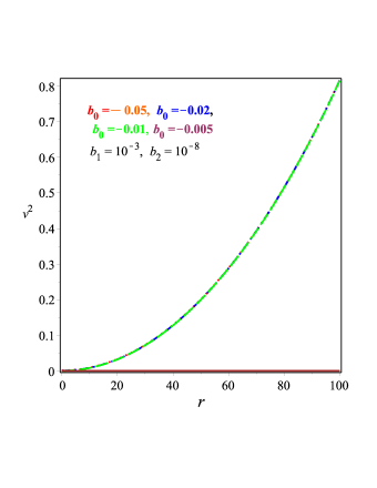
Figure 5: Speed of sound of (III) against $r$ in km.

We discuss the property of the speed of sound in the second solution because the first one gives a constant, which depends on the EoS parameter. Usually, the sound velocity must be less than the light speed Singh et al. (2019). Hence, in relativistic units, the sound speed must be less than or equal to unity. Thus, for the first solution, to give the sound speed less than or equal to unity, we must have $\omega_{t}\leq 1$. As Fig. 5 shows for solution (III), we have speed of sound less than 1 when the parameters $b_{1}=10^{-4}$ and $b_{2}=10^{-8}$.

IV Physics of the compact stars (III) and (III)

In this section, we explore the physical consequences for the first and second solutions given by Eqs. (III) and (III). To this end, first we are going to determine the values of the constants appearing in these solutions.

IV.1 Matching of boundary

We compare the solution within the compact objects with the Schwarzschild vacuum solution outside it. We use the first solution in Eq. (III) with the Schwarzschild one, i.e.,

$$ds^{2}=-\Big{(}1-\frac{2M}{r}\Big{)}dt^{2}+\Big{(}1-\frac{2M}{r}\Big{)}^{-1}dr^{2}+r^{2}d\Omega^{2}.$$ (42)

This yields the following matching conditions:

$$1-\frac{2M}{\cal{R}}=4\omega_{t}\ln({\cal{R}})+c_{1}\,,$$

$$\frac{1}{1-\frac{2M}{\cal{R}}}=\ln(4\omega_{t}+1)\,,$$ (43)

where ${\cal{R}}$ is the radius at the boundary, i.e., at the boundary $r={\cal{R}}$. Solving for $\omega_{t}$ and $c_{1}$ from Eq. (43), we obtain

$$\omega_{t}=\frac{e^{\frac{1}{1-\frac{2M}{\cal{R}}}}-1}{4}\,,\qquad\textrm{and }\qquad c_{1}=\frac{{\cal{R}}-2M+{\cal{R}}\ln\,{\cal{R}}-{\cal{R}}\ln\,{\cal{R}}{e^{\frac{1}{(1-\frac{2M}{\cal{R}})}}}}{\cal{R}}.$$ (44)

Here $M$ and ${\cal{R}}$ are determined by the observations of the compact objects. Applying the same procedure to the second solution (III) we get

$$b_{1}=\frac{2{\cal{R}}(1-b_{0})+5M}{{\cal{R}}^{3}}\,,\qquad\qquad b_{2}=\frac{3M-{\cal{R}}(1+b_{0})+5M}{{\cal{R}}^{5}}\,,$$ (45)

where $b_{0}$ is tackled by the data fitting and the values of $M$ and ${\cal{R}}$ are selected from the observations of the compact objects.

IV.2 Energy conditions for compact stars

In general, for perfect fluid models, the energy conditions described by the relation between the energy density and pressure can be satisfied. We check strong (SEC), weak (WEC), dominant (DEC) and finally null (NEC) energy conditions, given by

$$\textrm{SEC}:\rho+2p_{t}\geq 0\,,\qquad\qquad\qquad\qquad\textrm{NEC}:\rho+p_{t}\geq 0\,,$$

$$\textrm{WEC}:\rho\geq 0,\qquad\rho+p_{t}\geq 0\,,\qquad\qquad\textrm{DEC}:\rho\geq\mid p_{t}\mid\,.$$

By using Eqs. (III) and (III), one can easily show that the above conditions are satisfied as indicated in Figs. 6 5(a) and 5(b).

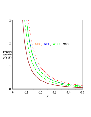
(a)  Energy conditions of solution (III) against radial coordinate

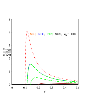
(b)  Energy conditions of solution (III) against radial coordinate

Figure 6: The energy conditions of solutions (III) and (III) against $r$ in km when $b_{1}=b_{2}=1$.

IV.3 Tolman-Oppenheimer-Volkoff equation and the analyses of the equilibrium

In this subsection we are going to discuss

We investigate how stable the models of the Einstein’s clusters are. We assume the equilibrium of the hydrostatic state. Through the Tolman-Oppenheimer-Volkoff (TOV) equation Tolman (1939); Oppenheimer and Volkoff (1939) as that presented in Ponce de Leon (1993), we acquire the equation

$$\frac{2p_{t}(r)}{r}-\frac{M_{g}(r)\rho(r)e^{(\mu-\nu)/2}}{r}=0\;,$$ (47)

with $M_{g}(r)$ the gravity mass as a function of $r$, which is defined by the Tolman-Whittaker mass formula as

$$M_{g}(r)=4\pi{\int_{0}}^{r}\Big{(}{T_{t}}^{t}-{T_{r}}^{r}-{T_{\theta}}^{\theta}-{T_{\phi}}^{\phi}\Big{)}r^{2}e^{(\mu+\nu)/2}dr=\frac{re^{(\nu-\mu)/2}\mu^{\prime}}{2}\,,$$ (48)

Using Eq. (48) in (47) we get

$$\frac{2p_{t}(r)}{r}-\frac{\mu^{\prime}\rho(r)}{2}=F_{g}+F_{a}=0\,,$$ (49)

with $F_{g}=-\frac{\mu^{\prime}\rho(r)}{2}$ being the gravitational force and $F_{a}=\frac{2p_{t}(r)}{r}$ is the anisotropic force. The behaviors of the TOV equations of solutions (III) and (III) are shown in Fig. 7 6(a) and 6(b), respectively.

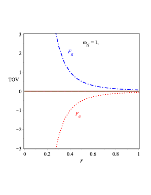
(a)  TOV of solution (III) against radial coordinate

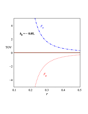
(b)  TOV of solution (III) against radial coordinate

Figure 7: TOV solutions (III) and (III) against $r$ in km when $b_{1}=b_{2}=1$.

IV.4 Relativistic adiabatic index and stability analysis

Our particular interest is to study the stable equilibrium configuration of a spherically symmetric cluster, and the adiabatic index is a basic ingredient of the stable/unstable criterion. Now considering an adiabatic perturbation, the adiabatic index $\Gamma$ is defined as Chandrasekhar (1964); Merafina and Ruffini (1989); Chan et al. (1993)

$$\Gamma=\frac{\rho+p_{t}}{p_{t}}\frac{dp_{t}}{d\rho}\,,$$ (50)

with $\frac{dp_{t}}{d\rho}$ is the speed of sound. Using Eq. (50) we get the adiabatic index of the two solutions (III) and (III) in the form:

$$\Gamma_{1}=1+\omega_{t1}\,,$$

$$\Gamma_{2}=\frac{(2b_{0}+3b_{1}r^{2}+4b_{2}r^{4})(3b_{0}b_{1}{}^{2}-45b_{1}{}^{2}b_{2}r^{4}-100b_{1}b_{2}{}^{2}r^{6}+32b_{0}b_{1}b_{2}r^{2}-100b_{2}{}^{3}r^{8}+60b_{0}b_{2}{}^{2}r^{4}-9b_{1}{}^{3}r^{2})}{2r^{2}(b_{1}+2b_{2}r^{2})(10b_{0}{}^{2}b_{2}-64b_{0}b_{1}b_{2}r^{2}-120b_{0}b_{2}{}^{2}r^{4}-45b_{1}{}^{2}b_{2}r^{4}-100b_{1}b_{2}{}^{2}r^{6}-50b_{2}{}^{3}r^{8}-15b_{0}b_{1}{}^{2}-9b_{1}{}^{3}r^{2})}\,.$$

The first set of Eq. (IV.4) is always larger than or equal to unity, depending on the value of EoS of $\omega_{t1}$. The behavior of the second set of Eq. (IV.4) is shown in Fig. 8. From this figure, we can see that the adiabatic index is always larger than unity and its value depends of the parameters $b_{0}$, $b_{1}$ and $b_{2}$.

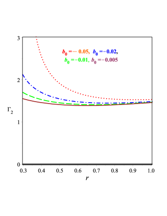
Figure 8: Adiabatic index of (III) against $r$ in km when $b_{1}=b_{2}=1$.

It has been found by Bondi Bondi (1964) that in the case of non-charged equilibrium, $\Gamma=4/3$ for the stable Newtonian sphere. It is shown in Haensel et al. (2007) that the variable range in terms of the value of $\Gamma$ is larger than or equal to 2 and less than or equal to 4 for the equations of state of most of the neutron stars.

IV.5 Stability in the static state

For stable compact stars, in terms of the mass-central as well as mass-radius relations for the energy density, Harrison, Zeldovich and Novikov [80, 81] claimed the gradient of the central density with respect to mass increase must be positive, i.e., $\frac{\partial M}{\partial\rho_{r_{0}}}>0$. If this condition is satisfied then we have stable configurations. To be more specific, stable or unstable region is satisfied for constant mass i.e. $\frac{\partial M}{\partial\rho_{r_{0}}}=0$. Let us apply this procedure to our solutions (III) and (III). To this end we calculate the central density for both solutions. For solution (III) the central density is undefined so we will exclude this case from our consideration because it may represent unstable configuration. As for the second solution the central density has the form

$$\rho_{r_{0}}=\frac{3b_{1}}{4\pi b_{0}}\Rightarrow b_{0}=\frac{3b_{1}}{4\pi\rho_{r_{0}}},$$

$$M(\rho_{r_{0}})=\frac{4\pi R^{3}\rho_{r_{0}}(b_{1}+2b_{2}R^{2})}{3b_{1}+12\pi b_{1}R^{2}\rho_{r_{0}}+20\pi b_{2}R^{4}\rho_{r_{0}}}\,.$$ (52)

With Eq. (IV.5) we have

$$\frac{\partial M}{\partial\rho_{r_{0}}}=\frac{12\pi R^{3}b_{1}(b_{1}+2b_{2}R^{2})}{(3b_{1}+12\pi b_{1}R^{2}\rho_{r_{0}}+20\pi b_{2}R^{4}\rho_{r_{0}})^{2}}\,.$$ (53)

From Eq. (53), it is seen that the solution (III) has a stable configuration since $\frac{\partial M}{\partial\rho_{r_{0}}}>0$. The behavior of the adiabatic index is shown in

Figure 9 depicts the mass in terms of the energy density. It follows from this figure that the mass increases as the energy density becomes larger.

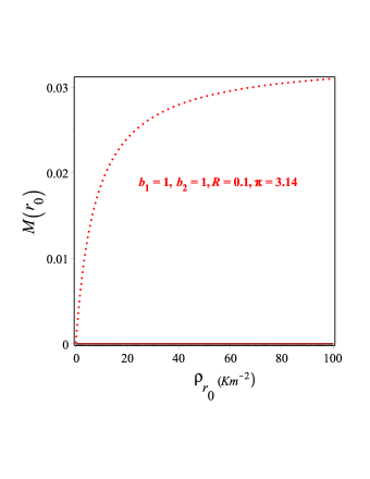
Figure 9: Static stability of (III) against $\rho_{r_{0}}$ in $\mathrm{km}^{-3}$ when $b_{1}=b_{2}=1,R=0.1$.

V Discussions and Conclusions

In this study, we have explored and discussed the model for compact stars which mimic clusters for TEGR. The gravitational field equations of the non-vacuum TEGR theory have been applied to a tetrad field with its non-diagonal components, which consists of functions of $\mu$ and $\nu$ possessing spherically symmetric fields. We have derived a set of the three equations with differentiations in terms of the five unknown quantities: $\mu$, $\nu$, $\rho$, $p_{r}$ and $p_{t}$. To be able to solve this system, we have put the radial pressure equal to zero Boehmer and Harko (2007); Singh et al. (2019) in addition to two different assumptions:

• In our first assumption we have taken an EoS between the density and the tangential pressure in the form $p_{t}=\omega_{{t_{1}}}\rho$. By using the vanishing of the pressure in the radial direction and the EoS parameter, we have solved the set of the differential equations and obtained two different solutions. One of these solutions is just the Schwarzschild exterior solution and we excluded it and the other one gave the unknown functions $\mu$, $\nu$, $\rho$ depending on the radial coordinate $r$, the parameter of EoS $\omega_{{t_{1}}}$ and on a constant of integration. We have studied the physics of this solution and shown that it has a positive density and pressure and a positive gravitational mass as shown in Figs. 1 1(a), 1 1(b) and 3 2(a). We have found that the speed of sound depends on the the parameter of EoS, $\omega_{t}$ which should be less than one, i.e., $\omega_{t}\leq 1$ Singh et al. (2019). We have also studied the boundary condition, i.e., matching our solution on the boundary with the exterior Schwarzschild solution, we derived the relations between the EoS parameter, the constant of integration and the gravitational mass of Schwarzschild and its radius at the boundary. Moreover, we showed that this solution satisfies all the energy conditions, i.e., SEC, WEC, DEC and NEC. As shown in Fig. 7 6(a), this solution satisfies the TOV equation. Finally, we have demonstrated that the adiabatic index of this solution is satisfied provided that $\omega_{t}\geq 1/3$ to have $\Gamma\geq 4/3$ Singh et al. (2019).

• In the second assumption, we have used a specific form of the unknown function $\mu$ that has three constants and derived the other unknown functions $\nu$, $\rho$ ad $p_{t}$. We have repeated the above procedure and shown that this solution has a positive density, a positive tangential pressure and a positive gravitational mass as shown in Figs. 2 1(a), 2 1(b) and 3 2(b). Also we have found that the sound speed depends on the radial coordinate and is always less than 1 as indicated in Fig. 5. The energy conditions of this solution are satisfied as shown in Fig. 6 5(b). We have matched our solution with the Schwarzschild exterior and derived a relation between two constants that characterize the unknown function $\mu$ with the gravitational mass and boundary radius of Schwarzschild and dealt with the third constant as a fitting parameter. Moreover, we showed that this solution satisfies the TOV equation as shown in Fig. 7 6(b). We have illustrated that the adiabatic index of this solution is satisfied and always has $\Gamma\geq 4/3$ as drawn in Fig. 8 Singh et al. (2019). Finally, we have demonstrated that the static stability is always satisfied because the derivative of the gravitational mass w.r.t. central density is always positive, indicating the gravitational mass increases with the central density as shown in Fig. 9.

To summarize, in the present paper we have used a non-diagonal form of tetrad field that gives null value of the off diagonal components of the field equations unlike what has been studied in the literature Ilijić and Sossich (2018); Abbas et al. (2015); Momeni et al. (2018); Abbas et al. (2015); Chanda et al. (2019); Debnath (2019); Ilijic and Sossich (2018). The results of this study give satisfactory physical compact stars as shown in the above discussion.

References

- Shekh and Chirde (2019) S. H. Shekh and V. R. Chirde, Gen. Rel. Grav. 51, 87 (2019).
- Perlmutter et al. (1999) S. Perlmutter, G. Aldering, G. Goldhaber, R. A. Knop, P. Nugent, P. G. Castro, S. Deustua, S. Fabbro, A. Goobar, D. E. Groom, I. M. Hook, A. G. Kim, M. Y. Kim, J. C. Lee, N. J. Nunes, R. Pain, C. R. Pennypacker, R. Quimby, C. Lidman, R. S. Ellis, M. Irwin, R. G. McMahon, P. Ruiz-Lapuente, N. Walton, B. Schaefer, B. J. Boyle, A. V. Filippenko, T. Matheson, A. S. Fruchter, N. Panagia, H. J. M. Newberg, W. J. Couch, and T. S. C. Project, Astrophys. J. 517, 565 (1999), astro-ph/9812133 .
- Spergel et al. (2007) D. N. Spergel et al. (WMAP), Astrophys. J. Suppl. 170, 377 (2007), arXiv:astro-ph/0603449 [astro-ph] .
- Hawkins et al. (2003) E. Hawkins, S. Maddox, S. Cole, O. Lahav, D. S. Madgwick, P. Norberg, J. A. Peacock, I. K. Baldry, C. M. Baugh, J. Bland-Hawthorn, T. Bridges, R. Cannon, M. Colless, C. Collins, W. Couch, G. Dalton, R. de Propris, S. P. Driver, G. Efstathiou, R. S. Ellis, C. S. Frenk, K. Glazebrook, C. Jackson, B. Jones, I. Lewis, S. Lumsden, W. Percival, B. A. Peterson, W. Sutherland, and K. Taylor, Monthly Notices of the Royal Astronomical Society 346, 78 (2003), http://oup.prod.sis.lan/mnras/article-pdf/346/1/78/9375978/346-1-78.pdf .
- Eisenstein et al. (2005) D. J. Eisenstein, I. Zehavi, D. W. Hogg, R. Scoccimarro, M. R. Blanton, R. C. Nichol, R. Scranton, H.-J. Seo, M. Tegmark, Z. Zheng, S. F. Anderson, J. Annis, N. Bahcall, J. Brinkmann, S. Burles, F. J. Castander, A. Connolly, I. Csabai, M. Doi, M. Fukugita, J. A. Frieman, K. Glazebrook, J. E. Gunn, J. S. Hendry, G. Hennessy, Z. Ivezić, S. Kent, G. R. Knapp, H. Lin, Y.-S. Loh, R. H. Lupton, B. Margon, T. A. McKay, A. Meiksin, J. A. Munn, A. Pope, M. W. Richmond, D. Schlegel, D. P. Schneider, K. Shimasaku, C. Stoughton, M. A. Strauss, M. SubbaRao, A. S. Szalay, I. Szapudi, D. L. Tucker, B. Yanny, and D. G. York, The Astrophysical Journal 633, 560 (2005).
- Aghanim et al. (2018) N. Aghanim et al. (Planck), (2018), arXiv:1807.06209 [astro-ph.CO] .
- Mazur and Mottola (2001) P. O. Mazur and E. Mottola, “Gravitational condensate stars: An alternative to black holes,” (2001), arXiv:gr-qc/0109035 [gr-qc] .
- Mazur and Mottola (2004) P. O. Mazur and E. Mottola, Proceedings of the National Academy of Sciences 101, 9545 (2004), https://www.pnas.org/content/101/26/9545.full.pdf .
- Usmani et al. (2011) A. Usmani, F. Rahaman, S. Ray, K. Nandi, P. K. Kuhfittig, S. Rakib, and Z. Hasan, Physics Letters B 701, 388 (2011).
- Rahaman et al. (2012a) F. Rahaman, A. A. Usmani, S. Ray, and S. Islam, Phys. Lett. B717, 1 (2012a), arXiv:1205.6796 [physics.gen-ph] .
- Rahaman et al. (2012b) F. Rahaman, S. Ray, A. Usmani, and S. Islam, Physics Letters B 707, 319 (2012b).
- Bhar (2014) P. Bhar, Astrophysics and Space Science 354, 457 (2014).
- Yousaf et al. (2019) Z. Yousaf, K. Bamba, M. Z. Bhatti, and U. Ghafoor, Phys. Rev. D100, 024062 (2019), arXiv:1907.05233 [gr-qc] .
- Copeland et al. (2006) E. J. Copeland, M. Sami, and S. Tsujikawa, Int. J. Mod. Phys. D15, 1753 (2006), arXiv:hep-th/0603057 [hep-th] .
- Papantonopoulos (2007) L. Papantonopoulos, ed., The invisible universe, Dark matter and dark energy. Proceedings, 3rd Aegean School, Karfas, Greece, September 26-October 1, 2005, Vol. 720 (2007).
- Bengochea and Ferraro (2009) G. R. Bengochea and R. Ferraro, Physical Review D 79 (2009), 10.1103/physrevd.79.124019.
- Cai et al. (2016) Y.-F. Cai, S. Capozziello, M. De Laurentis, and E. N. Saridakis, Rept. Prog. Phys. 79, 106901 (2016), arXiv:1511.07586 [gr-qc] .
- Bamba et al. (2012) K. Bamba, S. Capozziello, S. Nojiri, and S. D. Odintsov, Astrophys. Space Sci. 342, 155 (2012), arXiv:1205.3421 [gr-qc] .
- Saha and Debnath (2018) P. Saha and U. Debnath, Advances in High Energy Physics 2018, 1–13 (2018).
- De Felice and Tsujikawa (2010) A. De Felice and S. Tsujikawa, Living Reviews in Relativity 13, 3 (2010).
- Nojiri and Odintsov (2011) S. Nojiri and S. D. Odintsov, Phys. Rept. 505, 59 (2011), arXiv:1011.0544 [gr-qc] .
- Awad et al. (2017) A. M. Awad, S. Capozziello, and G. G. L. Nashed, JHEP 07, 136 (2017), arXiv:1706.01773 [gr-qc] .
- Capozziello and De Laurentis (2011) S. Capozziello and M. De Laurentis, Phys. Rept. 509, 167 (2011), arXiv:1108.6266 [gr-qc] .
- Nojiri et al. (2017) S. Nojiri, S. D. Odintsov, and V. K. Oikonomou, Phys. Rept. 692, 1 (2017), arXiv:1705.11098 [gr-qc] .
- Faraoni and Capozziello (2011) V. Faraoni and S. Capozziello, Beyond Einstein Gravity, Vol. 170 (Springer, Dordrecht, 2011).
- Bamba and Odintsov (2015) K. Bamba and S. D. Odintsov, Symmetry 7, 220 (2015), arXiv:1503.00442 [hep-th] .
- Ruiz-Lapuente (2010) P. Ruiz-Lapuente, Dark Energy: Observational and Theoretical Approaches (2010).
- Cognola et al. (2006) G. Cognola, E. Elizalde, S. Nojiri, S. D. Odintsov, and S. Zerbini, Phys. Rev. D73, 084007 (2006), arXiv:hep-th/0601008 [hep-th] .
- Harko et al. (2011) T. Harko, F. S. N. Lobo, S. Nojiri, and S. D. Odintsov, Phys. Rev. D84, 024020 (2011), arXiv:1104.2669 [gr-qc] .
- ARCOS and PEREIRA (2004) H. I. ARCOS and J. G. PEREIRA, International Journal of Modern Physics D 13, 2193–2240 (2004).
- El Hanafy and Nashed (2016) W. El Hanafy and G. G. L. Nashed, Astrophys. Space Sci. 361, 68 (2016), arXiv:1507.07377 [gr-qc] .
- Sotiriou et al. (2011) T. P. Sotiriou, B. Li, and J. D. Barrow, Physical Review D 83 (2011), 10.1103/physrevd.83.104030.
- Camera and Nishizawa (2013) S. Camera and A. Nishizawa, Physical Review Letters 110 (2013), 10.1103/physrevlett.110.151103.
- Aldrovandi and Pereira (2013) R. Aldrovandi and J. G. Pereira, Teleparallel Gravity: An Introduction, Fundamental Theories of Physics , Volume 173. ISBN 978-94-007-5142-2. Springer Science+Business Media Dordrecht, 2013 (2013).
- Nashed (2006) G. G. L. Nashed, Mod. Phys. Lett. , 2241 (2006), arXiv:gr-qc/0401041 [gr-qc] .
- Sahlu et al. (2019) S. Sahlu, J. Ntahompagaze, M. Elmardi, and A. Abebe, Eur. Phys. J. C79, 749 (2019), arXiv:1904.09897 [gr-qc] .
- Nashed (2003) G. G. L. Nashed, Chaos Solitons Fractals 15, 841 (2003), arXiv:gr-qc/0301008 [gr-qc] .
- Horvat et al. (2015) D. Horvat, S. Ilijić, A. Kirin, and Z. Narančić, Classical and Quantum Gravity 32, 035023 (2015).
- Shirafuji and Nashed (1997) T. Shirafuji and G. G. L. Nashed, Prog. Theor. Phys. 98, 1355 (1997), arXiv:gr-qc/9711010 [gr-qc] .
- Nashed (2010) G. G. L. Nashed, Chin. Phys. , 020401 (2010), arXiv:0910.5124 [gr-qc] .
- Liddle et al. (1994) A. R. Liddle, P. Parsons, and J. D. Barrow, Physical Review D 50, 7222–7232 (1994).
- Nashed (2008) G. G. L. Nashed, Int. J. Mod. Phys. A23, 1903 (2008), arXiv:0801.3548 [gr-qc] .
- Nashed (2019) G. Nashed, Int. J. Mod. Phys. D28, 1950158 (2019).
- Einstein (1939) A. Einstein, Annals of Mathematics 40, 922 (1939).
- Florides (1974) P. S. Florides, Proceedings of the Royal Society of London. Series A, Mathematical and Physical Sciences 337, 529 (1974).
- Zapolsky (1968) H. S. Zapolsky, apjl 153, L163 (1968).
- Gilhert (1954) C. Gilhert, Monthly Notices of the Royal Astronomical Society 114, 628 (1954), http://oup.prod.sis.lan/mnras/article-pdf/114/6/628/8074267/mnras114-0628.pdf .
- Comer and Katz (1993) G. L. Comer and J. Katz, Classical and Quantum Gravity 10, 1751 (1993).
- Mak and Harko (2003) M. K. Mak and T. Harko, Proceedings: Mathematical, Physical and Engineering Sciences 459, 393 (2003).
- Chaisi and Maharaj (2005) M. Chaisi and S. D. Maharaj, General Relativity and Gravitation 37, 1177–1189 (2005).
- Herrera et al. (2004) L. Herrera, A. Di Prisco, J. Martin, J. Ospino, N. O. Santos, and O. Troconis, Phys. Rev. D 69, 084026 (2004).
- Abreu et al. (2007) H. Abreu, H. Hernández, and L. A. Núñez, Classical and Quantum Gravity 24, 4631 (2007).
- Thirukkanesh and Maharaj (2008) S. Thirukkanesh and S. D. Maharaj, Classical and Quantum Gravity 25, 235001 (2008).
- Maurya et al. (2015) S. K. Maurya, Y. K. Gupta, S. Ray, and B. Dayanandan, The European Physical Journal C 75, 225 (2015).
- Folomeev and Dzhunushaliev (2015) V. Folomeev and V. Dzhunushaliev, Phys. Rev. D 91, 044040 (2015).
- Kalam et al. (2012) M. Kalam, F. Rahaman, S. Ray, S. M. Hossein, I. Karar, and J. Naskar, The European Physical Journal C 72, 2248 (2012).
- Maurya et al. (2019) S. K. Maurya, A. Banerjee, M. K. Jasim, J. Kumar, A. K. Prasad, and A. Pradhan, Phys. Rev. D 99, 044029 (2019).
- Bhar et al. (2017) P. Bhar, K. N. Singh, N. Sarkar, and F. Rahaman, The European Physical Journal C 77, 596 (2017).
- Bhar et al. (2016) P. Bhar, K. N. Singh, and T. Manna, Astrophysics and Space Science 361, 284 (2016).
- Singh et al. (2017) K. N. Singh, N. Pant, and M. Govender, Chinese Physics C 41, 015103 (2017).
- Böhmer and Harko (2006) C. G. Böhmer and T. Harko, Classical and Quantum Gravity 23, 6479 (2006).
- Andréasson and Böhmer (2009) H. Andréasson and C. G. Böhmer, Classical and Quantum Gravity 26, 195007 (2009).
- Maluf et al. (2002) J. W. Maluf, J. F. da Rocha-Neto, T. M. L. Toribio, and K. H. Castello-Branco, Phys. Rev. D65, 124001 (2002), arXiv:gr-qc/0204035 [gr-qc] .
- Nashed (2011) G. Nashed, Annalen der Physik 523, 450–458 (2011).
- Bahamonde et al. (2019) S. Bahamonde, K. Flathmann, and C. Pfeifer, (2019), arXiv:1907.10858 [gr-qc] .
- Boehmer and Harko (2007) C. G. Boehmer and T. Harko, Mon. Not. Roy. Astron. Soc. 379, 393 (2007), arXiv:0705.1756 [gr-qc] .
- Singh et al. (2019) K. N. Singh, F. Rahaman, and A. Banerjee, (2019), arXiv:1909.10882 [gr-qc] .
- Tolman (1939) R. C. Tolman, Phys. Rev. 55, 364 (1939).
- Oppenheimer and Volkoff (1939) J. R. Oppenheimer and G. M. Volkoff, Phys. Rev. 55, 374 (1939).
- Ponce de Leon (1993) J. Ponce de Leon, General Relativity and Gravitation 25, 1123 (1993).
- Chandrasekhar (1964) S. Chandrasekhar, Astrophys. J. 140, 417 (1964).
- Merafina and Ruffini (1989) M. Merafina and R. Ruffini, aap 221, 4 (1989).
- Chan et al. (1993) R. Chan, L. Herrera, and N. O. Santos, Monthly Notices of the Royal Astronomical Society 265, 533 (1993), http://oup.prod.sis.lan/mnras/article-pdf/265/3/533/3807712/mnras265-0533.pdf .
- Bondi (1964) H. Bondi, Proc. Roy. Soc. Lond. A281, 39 (1964).
- Haensel et al. (2007) P. Haensel, A. Y. Potekhin, and D. G. Yakovlev, Astrophys. Space Sci. Libr. 326, pp.1 (2007).
- Ilijić and Sossich (2018) S. c. v. Ilijić and M. Sossich, Phys. Rev. D 98, 064047 (2018).
- Abbas et al. (2015) G. Abbas, A. Kanwal, and M. Zubair, Astrophys. Space Sci. 357, 109 (2015), arXiv:1501.05829 [physics.gen-ph] .
- Momeni et al. (2018) D. Momeni, G. Abbas, S. Qaisar, Z. Zaz, and R. Myrzakulov, Can. J. Phys. 96, 1295 (2018), arXiv:1611.03727 [gr-qc] .
- Abbas et al. (2015) G. Abbas, S. Qaisar, and A. Jawad, apss 359, 17 (2015), arXiv:1509.06711 [physics.gen-ph] .
- Chanda et al. (2019) A. Chanda, S. Dey, and B. C. Paul, Eur. Phys. J. C79, 502 (2019).
- Debnath (2019) U. Debnath, Eur. Phys. J. C79, 499 (2019), arXiv:1901.04303 [gr-qc] .
- Ilijic and Sossich (2018) S. Ilijic and M. Sossich, Phys. Rev. D98, 064047 (2018), arXiv:1807.03068 [gr-qc] .