Flat Space, Dark Energy, and the Cosmic Microwave Background

Abstract

This paper reviews some of the results of the Planck collaboration and shows how to compute the distance from the surface of last scattering, the distance from the farthest object that will ever be observed, and the maximum radius of a density fluctuation in the plasma of the CMB. It then explains how these distances together with well-known astronomical facts imply that space is flat or nearly flat and that dark energy is 69% of the energy of the universe.

I Cosmic Microwave Background Radiation

The cosmic microwave background (CMB) was predicted by Gamow in 1948 [1], estimated to be at a temperature of 5 K by Alpher and Herman in 1950 [2], and discovered by Penzias and Wilson in 1965 [3]. It has been observed in increasing detail by Roll and Wilkinson in 1966 [4], by the Cosmic Background Explorer (COBE) collaboration in 1989–1993 [5, 6], by the Wilkinson Microwave Anisotropy Probe (WMAP) collaboration in 2001–2013 [7, 8], and by the Planck collaboration in 2009–2019 [9, 10, 11, 12].

The Planck collaboration measured CMB radiation at nine frequencies from 30 to 857 GHz by using a satellite at the Lagrange point L₂ in the Earth’s shadow some 1.5$\times 10^{6}$ km farther from the Sun [11, 12]. Their plot of the temperature $T(\theta,\phi)$ of the CMB radiation as a function of the angles $\theta$ and $\phi$ in the sky is shown in Fig. 1 with our galaxy outlined in gray. The CMB radiation is that of a 3000 K blackbody redshifted to $T_{0}=2.7255\pm 0.0006$K [13]. After correction for the motion of the Earth, the temperature of the CMB is the same in all directions apart from anisotropies of $300\,\upmu$K shown in red and blue. The CMB photons have streamed freely since the baryon-electron plasma cooled to 3000 K making hydrogen atoms stable and the plasma transparent. This time of initial transparency, some 380,000 years after the big bang, is called decoupling or recombination.

The CMB photons are polarized because they have scattered off electrons in the baryon-electron plasma before recombination and off electrons from interstellar hydrogen ionized by radiation from stars. The Planck collaboration measured the polarization of the CMB photons and displayed it in a graph reproduced in Fig. 2. They also used gravitational lensing to estimate the gravitational potential between Earth and the surface of last scattering. Their lensing map is shown in Fig. 3 with our galaxy in black.

Temperature fluctuations of the cosmic microwave background radiation

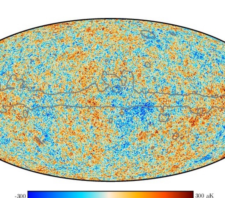
Figure 1: CMB temperature fluctuations over the celestial sphere as measured by the Planck satellite. The average temperature is 2.7255 K. The gray line outlines our galaxy. (arXiv:1807.06205 [astro-ph.CO], A&A doi.org/10.1051/0004-6361/201833880)

Polarization of the cosmic microwave background radiation

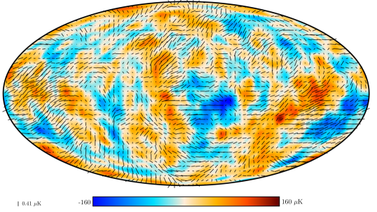
Figure 2: The polarization field superimposed upon the temperature map. (arXiv:1807.06205 [astro-ph.CO], A&A doi.org/10.1051/0004-6361/201833880)

The lensing map

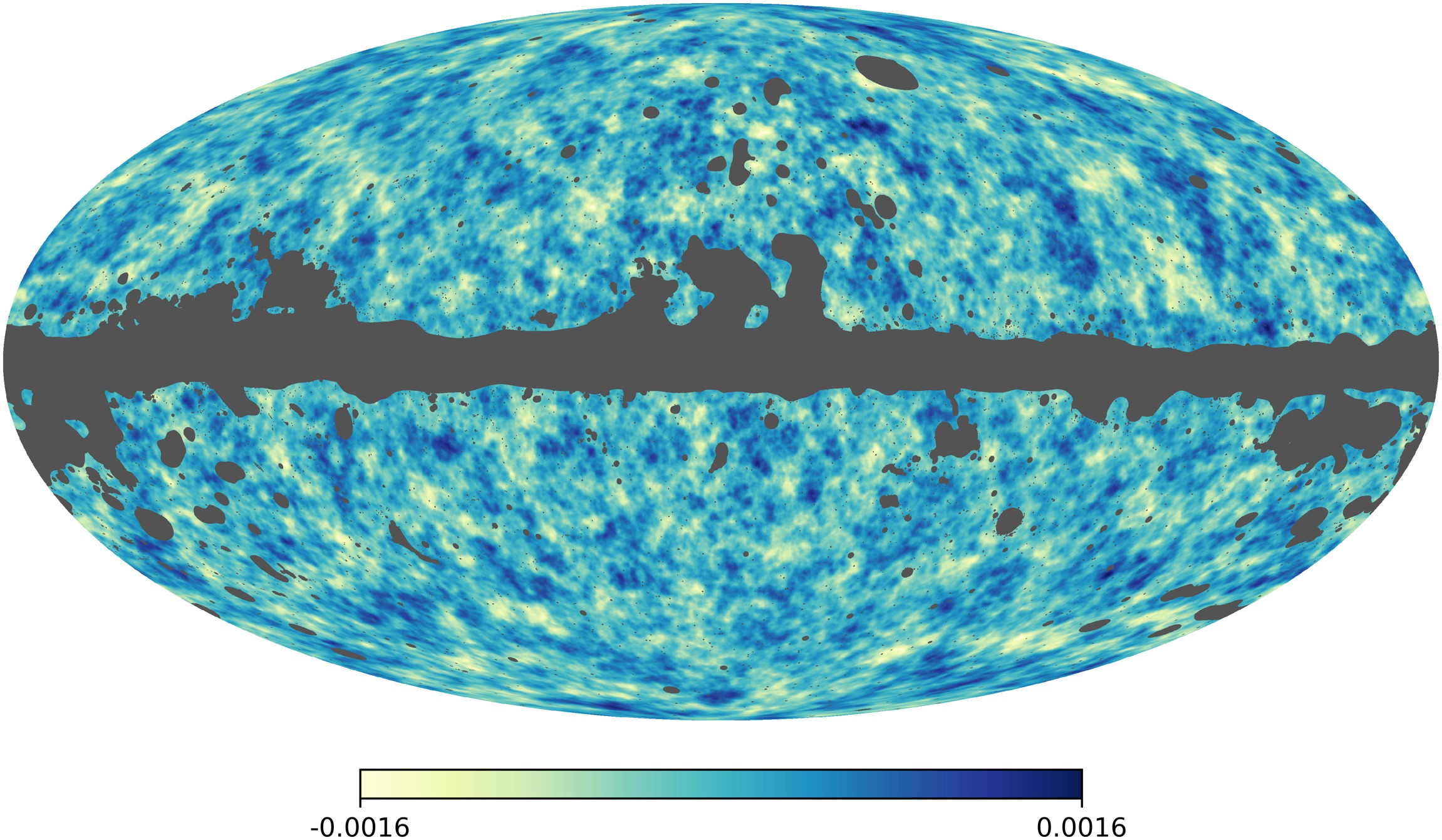
Figure 3: The gravitational potential between Earth and the surface of last scattering. (arXiv:1807.06205 [astro-ph.CO], A&A doi.org/10.1051/0004-6361/201833880)

Theoretical fit to the temperature anisotropies

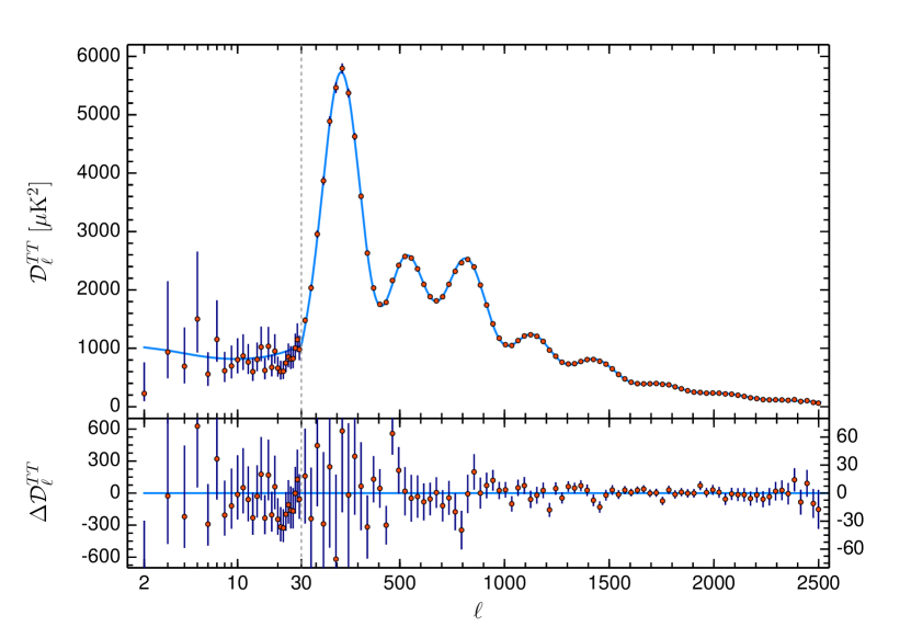
Figure 4: The temperature-temperature (TT) power spectrum $\mathcal{D}^{TT}_{\ell}=\ell(\ell+1)C_{\ell}/2\pi$ with its residuals in the lower panel is plotted against the multipole moment $\ell$ on a scale that goes from logarithmic to linear at $\ell=30$. The blue curve is the six-parameter $\Lambda$CDM fit. (Planck collaboration, arXiv:1807.06209)

The Planck collaboration expanded the temperature $T(\theta,\phi)$ they measured in spherical harmonics

$$T(\theta,\phi)=\sum_{\ell=0}^{\infty}\sum_{m=-\ell}^{\ell}a_{\ell,m}\,Y_{\ell,m}(\theta,\phi).$$ (1)

They used the coefficients

$$a_{\ell,m}=\int_{0}^{2\pi}\!\!d\phi\int_{0}^{\pi}\!\!\sin\theta\,d\theta\,\,\,Y^{*}_{\ell,m}(\theta,\phi)\,T(\theta,\phi)$$ (2)

to define a temperature-temperature (TT) power spectrum

$$\mathcal{D}^{TT}_{\ell}={}\frac{\ell(\ell+1)}{2\pi(2\ell+1)}\sum_{m=-\ell}^{\ell}|a_{\ell,m}|^{2}.$$ (3)

They similarly represented their measurements of CMB polarization and gravitational lensing as a temperature-polarization (TE) power spectrum $\mathcal{D}^{TE}_{\ell}$, a polarization-polarization (EE) power spectrum $\mathcal{D}^{EE}_{\ell}$, and a lensing spectrum $C^{\phi\phi}_{\ell}$. They were able to fit a simple, flat-space model of a universe with cold dark matter and a cosmological constant to their TT, TE, EE, and lensing data by using only six parameters. Their amazing fit to the TT spectrum is the blue curve plotted in Fig. 4.

The temperature-temperature power spectrum $\mathcal{D}^{TT}_{\ell}$ plotted in Fig. 4 is a snapshot at the moment of initial transparency of the temperature distribution of the rapidly expanding plasma of dark matter, baryons, electrons, neutrinos, and photons undergoing tiny ($2\times 10^{-4}$) acoustic oscillations. In these oscillations, gravity opposes radiation pressure, and $|\Delta T(\theta,\phi)|$ is maximal both when the oscillations are most compressed and when they are most rarefied. Regions that gravity has squeezed to maximum compression at transparency form the first and highest peak. Regions that have bounced off their first maximal compression and that have expanded under radiation pressure to minimum density at transparency form the second peak. Those at their second maximum compression at transparency form the third peak, and so forth. Decoupling was not instantaneous: the fractional ionization of hydrogen dropped from 0.236 at 334,600 years after the big bang to 0.0270 at 126,000 years later [14, p. 124]. The rapid high $\ell$ oscillations are out of phase with each other and are diminished.

The Planck collaboration found their data to be consistent with a universe in which space is flat but expanding due to the energy density of empty space (dark energy represented by a cosmological constant $\Lambda$). In their model, 84% of the matter consists of invisible particles (dark matter) that were cold enough to be nonrelativistic when the universe had cooled to $T\sim 10^{6}\,$K or $kT\sim 100$ eV. The Planck collaboration were able to fit their $\Lambda$-cold-dark-matter ($\Lambda$CDM) model as shown in Fig. 4 to their huge sets of data illustrated by Figs. 1–3 by adjusting only six cosmological parameters. In so doing, they determined the values of these six quantities: the present baryon density $\rho_{b0}$ (including nuclei and electrons), the present cold-dark-matter density $\rho_{d0}$, the angle $\theta_{s}$ subtended in the sky by disks whose radius is the sound horizon at recombination, the optical depth $\tau$ between Earth and the surface of last scattering, the amplitude $A_{s}$ of the fluctuations seen in Figs. 1–4, and the way $n_{s}$ in which fluctuations vary with their wavelength. Their estimates are [12, col. 7, p. 15]

$$\begin{array}[]{ll}\rho_{b0}=(4.211\pm 0.026)\times 10^{-28}\,\mbox{kg/m}^{3}&\rho_{d0}=(2.241\pm 0.017)\times 10^{-27}\,\mbox{kg/m}^{3}\\ \theta_{s}=0.0104101\pm 0.0000029&\tau=0.0561\pm 0.0071\\ \ln\left(10^{10}A_{s}\right)=3.047\pm 0.014&n_{s}=0.9665\pm 0.0038.\end{array}$$ (4)

They also estimated some 20 other cosmological parameters [12, col. 7, p. 15] and established flat $\Lambda$CDM as the standard model of cosmology.

Section II explains comoving coordinates, Friedmann’s equation, the critical density, and some basic cosmology. Section III explains how the scale factor $a(t)$, the redshift $z$, and the densities of matter, radiation, and empty space evolve with time and computes the comoving distance $r_{d}$ from the surface of decoupling or last scattering and the comoving distance from the most distant object that will ever be observed. Section IV computes the sound horizon $r_{s}$, which is the maximum size of an overdense fluctuation at the time of decoupling, and the angle $\theta_{s}=r_{s}/r_{d}$ subtended by it in the CMB. This calculation relates the first peak in the TT spectrum of Fig. 4 to the density of dark energy, the Hubble constant, and the age of the universe. Finally in section V it is shown that the angle $\theta_{s}=r_{s}/r_{d}$, which the Planck data determine as $\theta_{s}=0.0104101\pm 0.0000029$, varies by a factor of 146 when the Hubble constant is held fixed but the cosmological constant $\Lambda$ is allowed to vary from zero to twice the value determined by the Planck collaboration. This variation is mainly due to that of $r_{d}$ not $r_{s}$.

The paper does not discuss how the CMB anisotropies may have arisen from fluctuations in quantum fields before or during the big bang; this very technical subject is sketched by Guth [15, *Guth:2004tw, *Guth:2013epa] and described by Mukhanov, Feldman, and Brandenberger [18, 19] and by Liddle and Lyth [20].

II The Standard Model of Cosmology

On large scales, our universe is homogeneous and isotropic. A universe in which space is maximally symmetric [21, sec. 13.24] is described by a Friedmann-Lemaître-Robinson-Walker (FLRW) universe in which the invariant squared separation between two nearby points is

$$ds^{2}={}g_{ik}\,dx^{i}dx^{k}=-c^{2}dt^{2}+a^{2}(t)\,\left(\frac{dr^{2}}{1-k\,r^{2}/L^{2}}+r^{2}\,d\theta^{2}+r^{2}\,\sin^{2}\theta\,d\phi^{2}\right)$$ (5)

[22, 23, 24, 25], [21, sec. 13.42]. In this model, space (but not time) expands with a scale factor $a(t)$ that depends on time but not on position. Space is flat and infinite if $k=0$, spherically curved and finite if $k=1$, and hyperbolically curved and infinite if $k={}-1$. The curvature length $L$ lets us measure our comoving radial coordinate $r$ in meters.

Einstein’s equations imply Friedmann’s equation for the Hubble expansion rate $H=\dot{a}/a$

$$H^{2}=\left(\frac{\dot{a}}{a}\right)^{2}={}\frac{8\pi G}{3}\rho\,-\,\frac{c^{2}k}{a^{2}L^{2}}$$ (6)

in which $\rho$ is a mass density that depends on the scale factor $a(t)$, and the constant $G={}6.6743\times 10^{-11}$ m³ kg^-1 s^-2 is Newton’s [26]. The present value $H_{0}$ of the Hubble rate is the Hubble constant

$$H_{0}=\overline{H}_{0}\,\,h=100\,\,h\,\,\,\mbox{km/s/Mpc}=\left(3.24078\,\,\times 10^{-18}\,\,\mbox{s}^{-1}\right)\,\,h.$$ (7)

in which $h$ (not Planck’s constant) lies in the interval $0.67\lesssim h\lesssim 0.74$ according to recent estimates [12, 27, 28]. A million parsecs (Mpc) is $3.2616$ million lightyears (ly).

The critical density $\rho_{c}$ is the flat space density

$$\rho_{c}={}\frac{3H^{2}}{8\pi G}$$ (8)

which satisfies Friedmann’s equation (6) in flat ($k=0$) space

$$H^{2}=\left(\frac{\dot{a}}{a}\right)^{2}={}\frac{8\pi G}{3}\,\rho_{c}.$$ (9)

The present value of the critical density is

$$\rho_{c0}={}\frac{3H^{2}_{0}}{8\pi G}=\frac{3\overline{H}^{2}_{0}}{8\pi G}\,h^{2}=\left(1.87834\times 10^{-26}\,\,\mbox{kg/m}^{3}\right)\,\,h^{2}.$$ (10)

The present mass densities (4) of baryons $\rho_{b0}$ and of cold dark (invisible) matter $\rho_{d0}$ divided by the present value of the critical density $\rho_{c0}$ are the dimensionless ratios

$$\Omega_{b}=\frac{\rho_{b0}}{\rho_{c0}}\quad\mbox{and}\quad\Omega_{d}=\frac{\rho_{d0}}{\rho_{c0}}$$ (11)

in which the factor $h$ cancels. The Planck collaboration’s values for these ratios are [12]

$$\Omega_{b}\,h^{2}=0.02242\pm 0.00014\quad\mbox{and}\quad\Omega_{d}\,h^{2}=0.11933\pm 0.00091$$ (12)

in terms of which $\rho_{b0}={}[3\overline{H}_{0}^{2}/(8\pi G)]\,\,\Omega_{b}\,h^{2}$ and $\rho_{d0}={}[3\overline{H}_{0}^{2}/(8\pi G)]\,\,\Omega_{d}\,h^{2}$. The ratio of invisible matter to ordinary matter is $\Omega_{d}/\Omega_{b}=5.3$. The ratio for the combined mass density of baryons and dark matter is

$$\Omega_{bd}\,h^{2}={}{}\Omega_{b}\,h^{2}+\Omega_{d}\,h^{2}=0.14175.$$ (13)

The present density of radiation is determined by the present temperature $T_{0}=2.7255\pm 0.0006$  K [13] of the CMB and by Planck’s formula [21, ex. 5.14] for the mass density of photons

$$\rho_{\gamma 0}={}\frac{\pi^{2}\left(k_{B}T_{0}\right)^{4}}{15\,\hbar^{3}c^{5}}=4.645086\times 10^{-31}\,\,\mbox{kg m}^{-3}.$$ (14)

Adding in three kinds of massless Dirac neutrinos at $T_{0\nu}=(4/11)^{1/3}\,T_{0}$, we get for the present density of massless and nearly massless particles [14, sec. 2.1]

$$\rho_{r0}=\left[1+3\left(\frac{7}{8}\right)\left(\frac{4}{11}\right)^{4/3}\right]\,\,\rho_{\gamma}=7.809885\times 10^{-31}\,\,\mbox{kg m}^{-3}.$$ (15)

Thus the density ratio $\Omega_{r}\,h^{2}$ for radiation is

$$\Omega_{r}\,h^{2}={}\frac{\rho_{r0}}{\rho_{c0}}\,h^{2}=4.15787\times 10^{-5}.$$ (16)

If $k=0$, then space is flat and Friedmann’s equation (9) requires the density $\rho$ to always be the same as the critical density $\rho=\rho_{c}=3H^{2}/(8\pi G)$. The quantity $\Omega$ is the present density $\rho_{0}$ divided by the present critical density $\rho_{c0}$; in a $k=0$, spatially flat universe it is unity

$$\Omega\equiv\frac{\rho_{0}}{\rho_{c0}}=1.$$ (17)

The present density of baryons and dark matter $\rho_{bd}$ and that of radiation $\rho_{r0}$ do not add up to the critical density $\rho_{c0}$. In our $k=0$ universe, the difference is the density of empty space $\rho_{\Lambda}={}\rho_{c0}-\rho_{bd0}-\rho_{r0}$

$$\rho_{\Lambda}={}\rho_{c0}-\rho_{b0}-\rho_{d0}-\rho_{r0}.$$ (18)

Michael Turner called it dark energy. It is represented by a cosmological constant $\Lambda={}8\pi G\rho_{\Lambda}$ [29, 30].

Any departure from $k=0$ would imply a nonzero value for the curvature density $\rho_{k}=-3c^{2}k/(8\pi Ga^{2}L^{2})$ and for the dimensionless ratio

$$\Omega_{k}=\frac{\rho_{k0}}{\rho_{c0}}=-\frac{c^{2}k}{a^{2}_{0}H^{2}_{0}L^{2}}.$$ (19)

The WiggleZ dark-energy survey [31] used baryon acoustic oscillations to estimate this ratio as $\Omega_{k}={}-0.004\pm 0.006$; the WMAP [7, 8] collaboration found it to be $\Omega_{k}={}-0.0027\pm 0.0039$, consistent with zero, and the Planck collaboration [12] got the tighter bound

$$\Omega_{k}\equiv{}=0.0007\pm 0.0019.$$ (20)

For these reasons, the base model of the Planck collaboration has $k=0$, and I will use that value in Sections III and IV.

In flat space, time is represented by the real line and space by a 3-dimensional euclidian space that expands with a scale factor $a(t)$. In terms of comoving spherical and rectangular coordinates, the line element is

$$ds^{2}={}-c^{2}dt^{2}+a^{2}(t)\left(dr^{2}+r^{2}d\Omega^{2}\right)=-c^{2}dt^{2}+a^{2}(t)\left(dx^{2}+dy^{2}+dz^{2}\right)$$ (21)

where $d\Omega^{2}={}d\theta^{2}+\sin^{2}\theta\,d\phi^{2}$.

If light goes between two nearby points $\boldsymbol{r}$ and $\boldsymbol{r}^{\prime}$ in empty space in time $dt$, then the physical distance between the points is $c\,dt$. The flat-space invariant (21) gives that physical or proper distance as $c\,dt={}a(t)\sqrt{(\boldsymbol{r-r^{\prime}})^{2}}$. The corresponding comoving distance is $\sqrt{(\boldsymbol{r-r^{\prime}})^{2}}$.

Astronomers use coordinates in which the scale factor at the present time $t_{0}$ is unity $a(t_{0})=a_{0}=1$. In these coordinates, physical or proper distances at the present time $t_{0}$ are the same as comoving distances, $a(t_{0})\sqrt{(\boldsymbol{r-r^{\prime}})^{2}}=\sqrt{(\boldsymbol{r-r^{\prime}})^{2}}$.

A photon that is emitted at the time $t_{d}$ of decoupling at comoving coordinate $r_{d}$ and that comes to us through empty space along a path of constant $\theta,\phi$ has $ds^{2}=0$, and so the formula (21) for $ds^{2}$ gives

$$c\,dt={}-a(t)\,dr.$$ (22)

If our comoving coordinates now on Earth are $t_{0}$ and $r=0$, then the comoving radial coordinate of the emitting atom is

$$r_{d}={}\int_{0}^{r_{d}}dr={}\int_{t_{d}}^{t_{0}}\frac{c\,dt}{a(t)}.$$ (23)

The angle $\theta$ subtended by a comoving distance $\sqrt{(\boldsymbol{r-r^{\prime}})^{2}}$ that is perpendicular to the line of sight from the position $\boldsymbol{r}_{d}$ of the emitter to that of an observer now on Earth is

$$\theta={}\frac{\sqrt{(\boldsymbol{r-r^{\prime}})^{2}}}{r_{d}}.$$ (24)

To find the distance $r_{d}$, we need to know how the scale factor $a(t)$ varies with the time $t$.

III How the Scale Factor Evolves

This section begins with a discussion of how the densities of massive particles, of massless particles, and of dark energy vary with the scale factor. These densities and the assumed flatness of space will then be used to compute the distance from the surface of last scattering and the farthest distance that will ever be observed.

As space expands with the scale factor $a(t)$, the density of massive particles falls as

$$\rho_{bd}={}\frac{\rho_{bd0}}{a^{3}(t)}=\frac{\Omega_{bd}\,\rho_{c0}}{a^{3}(t)}.$$ (25)

Because wavelengths stretch with $a(t)$, the density $\rho_{r}$ of radiation falls faster

$$\rho_{r}={}\frac{\rho_{r0}}{a^{4}(t)}=\frac{\Omega_{r}\,\rho_{c0}}{a^{4}(t)}.$$ (26)

The density of empty space $\rho_{\Lambda}$ does not vary with the scale factor

$$\rho_{\Lambda}={}\Omega_{\Lambda}\,\rho_{c0}.$$ (27)

The Planck values for the density ratios are

$$\Omega_{bd}\,h^{2}=0.14175,\quad\Omega_{r}\,h^{2}=4.15787\times 10^{-5},\quad\mbox{and}\quad\Omega_{\Lambda}\,h^{2}=0.31537.$$ (28)

The last four equations let us estimate when the density of matter $\rho_{bd}$ first equaled that of radiation $\rho_{bd}=\rho_{r}$ as when

$$z+1=\frac{1}{a}={}\frac{\Omega_{bd}}{\Omega_{r}}=3409$$ (29)

and when the density of dark energy $\rho_{\Lambda}$ first equaled that of matter $\rho_{\Lambda}=\rho_{bd}$ as when

$$z+1=\frac{1}{a}={}\left(\frac{\Omega_{\Lambda}{}}{\Omega_{bd}}\right)^{1/3}=1.305.$$ (30)

To relate the red shift $z$ and the scale factor $a=1/(z+1)$ to the time since the moment of infinite redshift, we need to how the scale factor changes with time.

Friedmann’s equation for flat space (9) and the formula (10) for the critical density $\rho_{c0}$ give the square of the Hubble rate as

$$\begin{split}H^{2}={}&\frac{8\pi G}{3}\,\rho=\frac{8\pi G}{3}\,\left(\rho_{bd}+\rho_{r}+\rho_{\Lambda}\right)=\frac{8\pi G}{3}\,\left(\frac{\Omega_{bd}}{a^{3}}+\frac{\Omega_{r}}{a^{4}}+\Omega_{\Lambda}\right)\,\rho_{c0}\\ ={}&\frac{8\pi G}{3}\,\left(\frac{\Omega_{bd}}{a^{3}}+\frac{\Omega_{r}}{a^{4}}+\Omega_{\Lambda}\right)\frac{3\overline{H}_{0}^{2}}{8\pi G}\,h^{2}=\overline{H}_{0}^{2}\,\left(\frac{\Omega_{bd}\,h^{2}}{a^{3}}+\frac{\Omega_{r}\,h^{2}}{a^{4}}+\Omega_{\Lambda}\,h^{2}\right).\end{split}$$ (31)

This equation evaluated at the present time $t_{0}$ at which $H=H_{0}$ and $a(t_{0})=1$ is

$$H_{0}^{2}={}\overline{H}_{0}^{2}\,\left(\Omega_{bd}\,h^{2}+\Omega_{r}\,h^{2}+\Omega_{\Lambda}\,h^{2}\right)=H_{0}^{2}\,\left(\Omega_{bd}+\Omega_{r}+\Omega_{\Lambda}\right)$$ (32)

which restates the flat-space relation (17)

$$\Omega=\Omega_{bd}+\Omega_{r}+\Omega_{\Lambda}=1.$$ (33)

Using the formula (31) for $H$ and a little calculus

$$dt=\frac{da}{\dot{a}}=\frac{da}{a(\dot{a}/a)}=\frac{da}{aH},$$ (34)

we find as the time $t$ elapsed since $t=0$ when the scale factor was zero $a(0)=0$ as

$$t={}\int_{0}^{t}dt={}\int_{0}^{a(t)}\frac{da}{aH}={}\frac{1}{\overline{H}_{0}}\int_{0}^{a(t)}\frac{da}{\sqrt{\Omega_{\Lambda}\,h^{2}\,a^{2}+\Omega_{bd}\,h^{2}/a+\Omega_{r}\,h^{2}/a^{2}}}$$ (35)

in which the definition (7) of $\overline{H}_{0}$ is $\overline{H}_{0}=100$ km/s/Mpc $=3.24078\,\,\times 10^{-18}$ s^-1. Numerical integration leads to the values $z(t)$ and $a(t)$ plotted in Fig. 5.

Redshift and scalefactor over last 14 Gyr

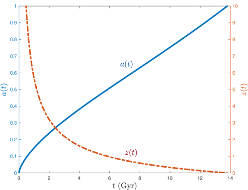
Figure 5: The scale factor $a(t)$ (solid, blue, left axis) and redshift $z(t)$ (dotdash, red, right axis) are plotted against the time in Gyr (Fig. 13.2 of [21], reprinted with permission).

Again using the formula (31) for $H$ and a little calculus

$$\frac{dt}{a}=\frac{da}{a\dot{a}}=\frac{da}{a^{2}(\dot{a}/a)}=\frac{da}{a^{2}H},$$ (36)

we find as the comoving distance travelled by a radially moving photon between $t_{1}$ and $t_{2}$

$$r_{2}-r_{1}={}\int_{t_{1}}^{t_{2}}\frac{c\,dt}{a(t)}={}\int_{a(t_{1})}^{a(t_{2})}\frac{c\,da}{a^{2}H}={}\frac{c}{\overline{H}_{0}}\int_{a(t_{1})}^{a(t_{2})}\frac{da}{\sqrt{\Omega_{\Lambda}\,h^{2}\,a^{4}+\Omega_{bd}\,h^{2}\,a+\Omega_{r}\,h^{2}}}.$$ (37)

Thus the comoving distance $r_{d}$ from the surface of last scattering at the time $t_{d}$ of decoupling at $a(t_{d})=1/1091$ to $r=0$ at $t_{0}$ is

$$r_{d}={}\int_{t_{d}}^{t_{0}}\frac{c\,dt}{a(t)}={}\frac{c}{\overline{H}_{0}}\int_{1/1091}^{1}\frac{da}{\sqrt{\Omega_{\Lambda}\,h^{2}\,a^{4}+\Omega_{bd}\,h^{2}\,a+\Omega_{r}\,h^{2}}}.$$ (38)

Substituting the values (28), we get as the distance from the surface of last scattering

$$r_{d}={}4.29171\times 10^{26}\,\mbox{m}=1.39085\times 10^{4}\,\,\mbox{Mpc}=4.53634\times 10^{10}\,\,\mbox{ly}.$$ (39)

At the time of decoupling, the physical distance $a(t_{d})r_{d}$ of the surface of last scattering from us was $a(t_{d})r_{d}=r_{d}/1091=4.16\times 10^{7}$ ly. A signal traveling that distance in time $t_{d}=3.8\times 10^{5}$ y would have had a speed of more than 100 $c$ [32]. Yet the the CMB coming to us from opposite directions is at almost the same temperature. Two explanations for this paradox are: that the hot big bang was preceded by a short period of superluminal expansion called inflation [33, 34] and that the universe equilibrated while collapsing before the hot big bang [35, 36] — a bouncing universe.

The scale factor is $a(0)=0$ at $t=0$, the time of infinite redshift, and is $a(\infty)=\infty$ at $t=\infty$ infinitely far in the future. Thus the comoving radial coordinate $r_{\infty}$ of the most distant emission of a photon that we could receive at $r=0$ if we waited for an infinitely long time is given by the integral

$$\begin{split}r_{\infty}={}&\int_{0}^{\infty}\frac{c\,dt}{a(t)}={}\frac{c}{\overline{H}_{0}}\int_{0}^{\infty}\frac{da}{\sqrt{\Omega_{\Lambda}\,h^{2}\,a^{4}+\Omega_{bd}\,h^{2}\,a+\Omega_{r}\,h^{2}}}\\ ={}&5.94739\times 10^{26}\,\mbox{m}=1.92742\times 10^{4}\,\,\mbox{Mpc}=6.2864\times 10^{10}\,\mbox{ly}\end{split}$$ (40)

which converges because of the vacuum-energy term $\Omega_{\Lambda}\,a^{4}$ in its denominator. Light emitted at the time of the big bang farther from Earth than 63 billion lightyears will never reach us because dark energy is accelerating the expansion of the universe.

IV The Sound Horizon

This section begins with a discussion of how rapidly changes in density can propagate in the hot plasma of dark matter, baryons, electrons, and photons before decoupling. This sound speed is then used to compute the maximum distance $r_{s}$ that a density fluctuation could propagate from the time of the big bang to the time of decoupling. The resulting sound horizon $r_{s}$ is the maximum radius of a fluctuation in the CMB. The angle subtended by such a fluctuation is the sound horizon divided by the distance $r_{d}$ (39) from the surface of last scattering, $\theta_{s}=r_{s}/r_{d}$. We will compute this angle as well as the Hubble constant and the age of the universe by using the Planck values for the densities of matter, radiation, and dark energy, and the assumption that space is flat.

Before photons decoupled from electrons and baryons, the oscillations of the plasma of dark matter, baryons, electrons, and photons were contests between gravity and radiation pressure. Because photons vastly outnumber baryons and electrons, the photons determined the speed of sound $v_{s}$ in the plasma. The pressure $p$ of a gas of photons is one-third of its energy density $p=\rho\,c^{2}/3$, and so the speed of sound due to the photons is [37, Sec. iii.6]

$$v_{s}=\left(\frac{\delta p}{\delta\rho}\right)^{1/2}=\frac{c}{\sqrt{3}}.$$ (41)

A better estimate of the speed of sound is one that takes into account the baryons [14, ch. 2]

$$v_{s}=\frac{c}{\sqrt{3}}\frac{1}{\sqrt{1+R}}$$ (42)

in which $R$ is proportional to the baryon density (4) divided by the photon density (14)

$$R=\frac{3\rho_{b}}{4\rho_{\gamma}}=\frac{3\rho_{b0}}{4\rho_{\gamma 0}}\,a=678.435\,a.$$ (43)

The sound horizon $r_{s}$ is the comoving distance that a pressure or sound wave could travel between the time of infinite redshift and the time of decoupling. The high-density bubble is a sphere, so we can compute the distance $r_{s}$ for constant $\theta,\phi$. Using the ratios $\Omega_{bd}$ and $\Omega_{r}$ in the distance integral (37) with lower limit $a(0)=0$ and upper limit $a_{d}=1/1091$ and with the speed of light $c$ replaced by the speed of sound $v_{s}$ (42 and 43), we get

$$\begin{split}r_{s}={}&\int_{0}^{t_{d}}\frac{c\,dt}{\sqrt{3(1+R)}\,a(t)}={}\frac{c}{\sqrt{3}\,\,\overline{H}_{0}}\int^{1/1091}_{0}\frac{da}{\sqrt{(1+R)(\Omega_{\Lambda}\,h^{2}\,a^{4}+\Omega_{bd}\,h^{2}\,a+\Omega_{r}\,h^{2})}}.\end{split}$$ (44)

Substituting the values $\Omega_{bd}\,h^{2}=0.14175$, $\Omega_{r}\,h^{2}=4.15787\times 10^{-5}$, and $\Omega_{\Lambda}\,h^{2}=0.31537$, we find for the sound horizon

$$r_{s}={}4.4685\times 10^{24}\,\mbox{m}=144.814\,\mbox{Mpc}=4.72321\times 10^{8}\,\,\mbox{ly}.$$ (45)

The angle subtended by the sound horizon $r_{s}$ at the distance $r_{d}$ is the ratio

$$\theta_{s}={}\frac{r_{s}}{r_{d}}=0.0104119$$ (46)

which is exactly the Planck result $\theta_{P}={}0.0104119\pm 0.0000029$, a measurement with a precision of 0.03 % [12]. It is the location of the first peak in the TT spectrum of Fig. 4. Had we done this calculation (38 and 44) of the angle $\theta_{s}$ for a variety of values for the dark-energy density $\Omega_{\Lambda}h^{2}$, we would have found $\Omega_{\Lambda}h^{2}=0.31537$ as the best density. Thus the Planck measurement of $\theta_{s}$ together with the flatness of space and the densities of matter and radiation determine the density of dark energy.

The formula (31) for the Hubble rate in terms of the densities gives the Hubble constant as

$$H_{0}={}\overline{H}_{0}\sqrt{\Omega_{\Lambda}\,h^{2}+\Omega_{bd}\,h^{2}+\Omega_{r}\,h^{2}}={}67.614\,\,\mbox{km s}^{-1}\,\mbox{Mpc}^{-1}=2.19121\times 10^{-18}\,\,\mbox{s}^{-1}.$$ (47)

This value is well within $1\sigma$ of the value found by the Planck collaboration $H_{0}={}67.66\pm 0.42$ km/s/Mpc [12]. The Planck value for $H_{0}$ reflects the physics of the universe between the big bang and decoupling some 380,000 years later. Using the Hubble Space Telescope to observe 70 long-period Cepheids in the Large Magellanic Cloud, the Riess group recently found [27] $H_{0R}={}74.03\pm 1.42$ km/s/Mpc, a value that reflects the physics of the present universe. More recently, using a calibration of the tip of the red giant branch applied to Type Ia supernovas, the Freedman group found [28] $H_{0F}={}69.8\pm 0.8$ km/s/Mpc, another value that reflects the physics of the present universe.

Finally, using the formula (31) for the Hubble rate $H=\dot{a}/a$ in terms of the density ratios, we can write the age of the universe as an integral of $dt=da/(aH)$ from $a(0)=0$ to $a(t_{0})=1$

$$t_{0}={} \int_{0}^{1}\frac{da}{aH}=\int_{0}^{1}\frac{da}{\overline{H}_{0}\sqrt{\Omega_{\Lambda}\,h^{2}\,a^{2}+\Omega_{bd}\,h^{2}\,a^{-1}+\Omega_{r}\,h^{2}\,a^{-2}}}$$ (48)

$$={} 4.35756\times 10^{17}\,\mbox{s}=13.808\times 10^{9}\,\,\mbox{sidereal years},$$ (49)

which is within $1\sigma$ of the Planck collaboration’s value $t_{0}=(13.787\pm 0.020)\times 10^{9}$ y [12].

V Sensitivity of the Sound Horizon to $\Lambda$

In this section, keeping the Hubble constant fixed but relaxing the assumption that space is flat, we will compute the distances $r_{s}$ and $r_{d}$ and the angle $\theta_{s}=r_{s}/r_{d}$ for different values of the dark-energy density. We will find that although the sound horizon $r_{s}$ remains fixed, the distance $r_{d}$ and the angle $\theta_{s}$ vary markedly as the cosmological constant runs from zero to twice the Planck value. This wide variation supports the conclusion that space is flat and that the dark-energy density is close to the Planck value.

Since astronomical observations have determined the value of the Hubble constant $H_{0}$ to within 10%, we will keep it fixed at the value estimated by the Planck collaboration while varying the density of dark energy and seeing how that shifts the position $\theta_{s}$ of the first peak of the TT spectrum of Fig. 4. Since the energy density will not be equal to the critical density, space will not be flat, so we must use the Friedmann equation (6)

$$H^{2}=\left(\frac{\dot{a}}{a}\right)^{2}={}\frac{8\pi G}{3}\,\rho-\frac{c^{2}k}{a^{2}L^{2}}=\overline{H}_{0}^{2}\,\left(\frac{\Omega_{bd}\,h^{2}}{a^{3}}+\frac{\Omega_{r}\,h^{2}}{a^{4}}+\Omega_{\Lambda_{k}}\,h^{2}\right)-\frac{c^{2}k}{a^{2}L^{2}}$$ (50)

which includes a curvature term instead of the flat-space Friedmann equation (6). Since we are holding the Hubble constant $H_{0}$ fixed, the curvature term $-c^{2}k/(a_{0}^{2}L^{2})$ must compensate for the change of the cosmological-constant ratio to $\Omega_{\Lambda_{k}}$ from the Planck value $\Omega_{\Lambda}=0.6889\pm 0.0056$ [12]. We can find the needed values of $k$ and $L$ by using the equation (31) for the Hubble constant. We require

$$H_{0}^{2}={}\overline{H}_{0}^{2}\,\left(\Omega_{bd}\,h^{2}+\Omega_{r}\,h^{2}+\Omega_{\Lambda}\,h^{2}\right)=\overline{H}_{0}^{2}\,\left(\Omega_{bd}\,h^{2}+\Omega_{r}\,h^{2}+\Omega_{\Lambda_{k}}\,h^{2}\right)-\frac{c^{2}k}{a^{2}_{0}L^{2}}$$ (51)

or

$$\frac{c^{2}k}{a^{2}_{0}L^{2}}={}\overline{H}_{0}^{2}\,h^{2}\left(\Omega_{\Lambda_{k}}-\Omega_{\Lambda}\right)\quad\mbox{and}\quad L={}\frac{c}{a_{0}H_{0}|\Omega_{\Lambda_{k}}-\Omega_{\Lambda}|}$$ (52)

in which $k=(\Omega_{\Lambda_{k}}-\Omega_{\Lambda})/|\Omega_{\Lambda_{k}}-\Omega_{\Lambda}|=\pm 1$. With these values of $k$ and $L$, Friedmann’s equation (50) is

$$\begin{split}H^{2}={}&\left(\frac{\dot{a}}{a}\right)^{2}={}\overline{H}^{2}_{0}\,\left(\frac{\Omega_{bd}\,h^{2}}{a^{3}}+\frac{\Omega_{r}\,h^{2}}{a^{4}}+\Omega_{\Lambda_{k}}\,h^{2}\right)-\frac{c^{2}k}{a^{2}L^{2}}\\ ={}&\overline{H}^{2}_{0}\,\left(\frac{\Omega_{bd}\,h^{2}}{a^{3}}+\frac{\Omega_{r}\,h^{2}}{a^{4}}+\Omega_{\Lambda_{k}}\,h^{2}\left(1-\frac{1}{a^{2}}\right)+\Omega_{\Lambda}\,h^{2}\right).\end{split}$$ (53)

Now since $k\neq 0$ when $\Omega_{\Lambda}$ is replaced by $\Omega_{\Lambda_{k}}$, the relation (23) between $cdt$ and an element $dr$ of the radial comoving coordinate becomes the one that follows from $ds^{2}=0$ when the FLRW formula (5) for $ds^{2}$ applies

$$\frac{c\,dt}{a(t)}={}\pm\frac{dr}{\sqrt{1-kr^{2}/L^{2}}}.$$ (54)

The minus sign is used for a photon emitted during decoupling at $t=t_{d}$ on the surface of last scattering at $r=r_{d}$ and absorbed here at $r=0$ and $t=t_{0}$. Integrating, we get as the scaled distance $D(t_{0},t_{d})$ traveled by a photon emitted at comoving coordinate $r_{d}$ at time $t_{d}$ and observed at $r=0$ at time $t_{0}$

$$D(t_{d},t_{0})\equiv\int_{t_{d}}^{t_{0}}\frac{c\,dt}{a(t)}={}\int_{0}^{r_{d}}\frac{dr}{\sqrt{1-kr^{2}/L^{2}}}={}\left\{\begin{array}[]{ll}L\operatorname{arcsinh}\big{(}r_{d}/L\big{)}&\quad\mbox{if }k=-1\\ r_{d}&\quad\mbox{if }k=0\\ L\arcsin\big{(}r_{d}/L\big{)}&\quad\mbox{if }k=1\end{array}\right..$$ (55)

Inverting these formulas (55), we find the comoving coordinate $r_{d}$ of emission

$$r_{d}={}\left\{\begin{array}[]{ll}L\sinh\big{(}D(t_{d},t_{0})/L\big{)}&\quad\mbox{if }k=-1\\ D(t_{d},t_{0})&\quad\mbox{if }k=0\\ L\sin\big{(}D(t_{d},t_{0})/L\big{)}&\quad\mbox{if }k=1\end{array}\right..$$ (56)

Using again the relation (36) $dt/a=da/(a^{2}H)$ and the formula (53) for the Hubble rate, we find as the scaled distance (55) traveled by a photon from the surface of last scattering at the time of decoupling

$$\begin{split}D(t_{d},t_{0})={}&\int_{t_{d}}^{t_{0}}\frac{c\,dt}{a(t)}={}\int_{1/1091}^{1}\frac{da}{a^{2}H}\\ ={}&\frac{c}{\overline{H}_{0}}\int_{1/1091}^{1}\frac{da}{\sqrt{\Omega_{bd}\,h^{2}\,a+\Omega_{r}\,h^{2}+\Omega_{\Lambda_{k}}\,h^{2}\left(a^{4}-a^{2}\right)+\Omega_{\Lambda}\,h^{2}\,a^{4}}}.\end{split}$$ (57)

Positions of the first peak for various cosmological constants $\Lambda_{k}$
$\Lambda_{k}$	$k$	$r_{s}$ (Mpc)	$r_{d}$ (Gpc)	angle $\theta_{s}$	multipole $\ell$
$2\Lambda$	$1$	145	1.53	0.0947	25
$3\Lambda/2$	$1$	145	6.87	0.021	110
$\Lambda$	$0$	145	13.9	0.0104	220
$2\Lambda/3$	${}-1$	145	23.2	0.00624	370
$\Lambda/2$	${}-1$	145	27.9	0.00518	450
$\Lambda/3$	${}-1$	145	33.3	0.00435	530
$\Lambda/4$	${}-1$	145	36.2	0.00400	580
$0$	${}-1$	145	221	0.00065	3550

Table 1: The values of the parameter $k$, of the comoving coordinates of the sound horizon $r_{s}$ and of the surface of last scattering $r_{d}$, the angle $\theta_{s}=r_{s}/r_{d}$, and the approximate multipole moment of the first peak in the TT spectrum are listed for several values of the cosmological constant $\Lambda_{k}$.

Sensitivity of the first peak to the value of the cosmological constant

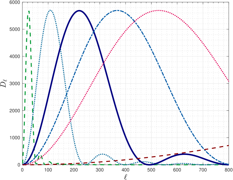
Figure 6: The TT spectra of a sky that is dark except for a single disk at $\theta=0$ that subtends an angle $\theta_{s}=r_{s}/r_{d}$ that is the ratio of the sound horizon $r_{s}$ to the distance $r_{d}$ from the surface of last scattering for various values of the cosmological constant $\Lambda_{k}$ with the Hubble constant $H_{0}$ held fixed. From left to right, the peaks are at $\ell\approx 25$ and $\theta=0.095$ for $\Lambda_{k}=2\Lambda$ (dashes, green), at $\ell\approx 110$ and $\theta=0.021$ for $\Lambda_{k}=3\Lambda/2$ (dots, bluegreen), at $\ell\approx 220$ and $\theta=0.0104$ for $\Lambda_{k}=\Lambda$ (solid, dark blue), at $\ell\approx 370$ and $\theta=0.00624$ for $\Lambda_{k}=2\Lambda/3$ (dot-dash, teal), at $\ell\approx 530$ and $\theta=0.00435$ for $\Lambda_{k}=\Lambda/3$ (dots, raspberry), and off scale at $\ell\approx 3550$ and $\theta=0.00065$ for $\Lambda=0$ (dashes, dark red). The spectra are scaled so as to have the same maximum value.

We use the plus sign in the relation (54) between $dt$ and $dr$ for a photon emitted in the big bang at $r=0$ and absorbed at $r_{s}$ at $t_{d}$. So using again the relation (36) $dt/a=da/(a^{2}H)$ and the formula (53) for the Hubble rate, we find the scaled distance a sound wave could go starting at the big bang and stopping at decoupling would be

$$D(0,t_{d})={} \frac{c}{\overline{H}_{0}}\int^{1/1091}_{0}\!\!\!\!\!\frac{da}{\sqrt{3(1+R)(\Omega_{bd}\,h^{2}\,a+\Omega_{r}\,h^{2}+\Omega_{\Lambda_{k}}\,h^{2}\left(a^{4}-a^{2}\right)+\Omega_{\Lambda}\,h^{2}\,a^{4})}}.$$ (58)

The inversion formulas (56) then give the comoving coordinates $r_{d}$ and $r_{s}$ and the angle $\theta_{s}=r_{s}/r_{d}$ corresponding to $D(t_{0},t_{d})$ and $D(t_{d},0)$.

I used these formulas (56–58) to find the angles $\theta_{s}$ and comoving coordinates $r_{s}$ and $r_{d}$ that result when the cosmological constant is changed from the Planck value $\Lambda$ to $\Lambda_{k}$. The resulting values of $k,r_{s},r_{d},\theta_{s}=r_{s}/r_{d},$ and the approximate positions of the first peak in the resulting TT spectrum are listed in Table 1 for several values of the cosmological constant $\Lambda_{k}$. The position $r_{d}$ of the surface of last scattering varies by a factor of 144, and the angle $\theta_{s}$ varies by a factor of 146. The sound horizon $r_{s}$ is almost independent of $\Lambda_{k}$ because in the integral 58) for $D(t_{d},0)$, the scale factor $a$ is less than $1/1091$, and the ratios $\Omega_{\Lambda}$ and $\Omega_{\Lambda_{k}}$ are respectively multiplied by $a^{4}\sim 10^{-12}$ and by $a^{4}-a^{2}\sim{}-10^{-6}$.

To see how the first peak of the TT spectrum might vary with the cosmological constant $\Lambda_{k}$, I used a toy CMB consisting of a single disk whose radius subtends the angle $\theta_{s}=r_{s}/r_{d}$. For such a disk about the north pole from $\theta=0$ to $\theta=\theta_{s}$, only the $m=0$ term in the formula (2) for $a_{\ell m}$ contributes, and so

$$a_{\ell 0}={}\sqrt{\pi(2\ell+1)}\int_{-1}^{1}dx\,P_{\ell}(x)\,T(x)\quad\mbox{and}\quad D_{\ell}=\frac{\ell(\ell+1)}{2}\left|\int_{x_{s}}^{1}dx\,P_{\ell}(x)\,T(x)\right|^{2}$$ (59)

in which $x_{s}=\cos\theta_{s}$. To avoid a sharp cutoff at $x=\cos\theta_{s}$, I chose as the temperature distribution across the disk $T(x)={}A\left[1-\cos^{2}(\theta_{s})/x^{2}\right]$ which drops smoothly to zero across the disk. The resulting TT spectra for cosmological constants $\Lambda_{k}$ equal to the Planck value $\Lambda$ multiplied by 2, 3/2, 1, 2/3, 1/3, or 0 are plotted in Fig. 6. The Hubble constant was held fixed at the Planck value.

References

- Gamow [1948] G. Gamow, The Origin of Elements and the Separation of Galaxies, Phys. Rev. 74, 505 (1948).
- Alpher and Herman [1950] R. A. Alpher and R. C. Herman, Theory of the Origin and Relative Abundance Distribution of the Elements, Rev. Mod. Phys. 22, 153 (1950).
- Penzias and Wilson [1965] A. A. Penzias and R. W. Wilson, A Measurement of excess antenna temperature at 4080-Mc/s, Astrophys. J. 142, 419 (1965).
- Roll and Wilkinson [1966] P. G. Roll and D. T. Wilkinson, Cosmic Background Radiation at 3.2 cm-Support for Cosmic Black-Body Radiation, Phys. Rev. Lett. 16, 405 (1966).
- Mather et al. [1990] J. C. Mather et al., A Preliminary measurement of the Cosmic Microwave Background spectrum by the Cosmic Background Explorer (COBE) satellite, Astrophys. J. 354, L37 (1990).
- Smoot et al. [1992] G. F. Smoot et al. (COBE), Structure in the COBE differential microwave radiometer first year maps, Astrophys. J. 396, L1 (1992).
- Peiris et al. [2003] H. V. Peiris et al. (WMAP), First year Wilkinson Microwave Anisotropy Probe (WMAP) observations: Implications for inflation, Astrophys. J. Suppl. 148, 213 (2003), arXiv:astro-ph/0302225 [astro-ph] .
- Bennett et al. [2013] C. L. Bennett et al. (WMAP), Nine-Year Wilkinson Microwave Anisotropy Probe (WMAP) Observations: Final Maps and Results, Astrophys. J. Suppl. 208, 20 (2013), arXiv:1212.5225 [astro-ph.CO] .
- Ade et al. [2014] P. A. R. Ade et al. (Planck), Planck 2013 results. XVI. Cosmological parameters, Astron. Astrophys. 571, A16 (2014), arXiv:1303.5076 [astro-ph.CO] .
- Ade et al. [2016] P. A. R. Ade et al. (Planck), Planck 2015 results. XIII. Cosmological parameters, Astron. Astrophys. 594, A13 (2016), arXiv:1502.01589 [astro-ph.CO] .
- Akrami et al. [2018] Y. Akrami et al. (Planck), Planck 2018 results. I. Overview and the cosmological legacy of Planck (2018), A&A doi.org/10.1051/0004-6361/201833880, arXiv:1807.06205 [astro-ph.CO] .
- Aghanim et al. [2018] N. Aghanim et al. (Planck), Planck 2018 results. VI. Cosmological parameters (2018), arXiv:1807.06209 [astro-ph.CO] .
- Fixsen [2009] D. J. Fixsen, The temperature of the cosmic microwave background, Astrophys. J. 707, 916 (2009), arXiv:0911.1955 [astro-ph.CO] .
- Weinberg [2010] S. Weinberg, Cosmology (Oxford University Press, 2010).
- Guth [2003] A. H. Guth, Inflation and cosmological perturbations, in The future of theoretical physics and cosmology: Celebrating Stephen Hawking’s 60th birthday. Proceedings, Workshop and Symposium, Cambridge, UK, January 7-10, 2002 (2003) pp. 725–754, arXiv:astro-ph/0306275 [astro-ph] .
- Guth [2004] A. H. Guth, Inflation, in Measuring and modeling the universe. Proceedings, Symposium, Pasadena, USA, November 17-22, 2002 (2004) pp. 31–52, arXiv:astro-ph/0404546 [astro-ph] .
- Guth [2013] A. H. Guth, Quantum Fluctuations in Cosmology and How They Lead to a Multiverse, in Proceedings, 25th Solvay Conference on Physics: The Theory of the Quantum World: Brussels, Belgium, October 19-25, 2011 (2013) arXiv:1312.7340 [hep-th] .
- Mukhanov et al. [1992] V. F. Mukhanov, H. A. Feldman, and R. H. Brandenberger, Theory of cosmological perturbations. Part 1. Classical perturbations. Part 2. Quantum theory of perturbations. Part 3. Extensions, Phys. Rept. 215, 203 (1992).
- Mukhanov [2005] V. Mukhanov, Physical Foundations of Cosmology (Cambridge University Press, Oxford, 2005).
- Liddle and Lyth [1993] A. R. Liddle and D. H. Lyth, The Cold dark matter density perturbation, Phys. Rept. 231, 1 (1993), arXiv:astro-ph/9303019 [astro-ph] .
- Cahill [2019] K. Cahill, Physical Mathematics, 2nd ed. (Cambridge University Press, 2019).
- Friedmann [1922] A. Friedmann, Über die krümmung des raumes, Z. Phys. 10, 377 (1922).
- Lemaître [1927] G. Lemaître, Ann. Soc. Sci. Brux. A47, 49 (1927).
- Robertson [1935] H. P. Robertson, Ap. J. 82, 284 (1935).
- Walker [1936] A. G. Walker, Proc. Lond. Math. Soc. (2) 42, 90 (1936).
- Tiesinga et al. [2019] E. Tiesinga, P. J. Mohr, D. B. Newell, and B. N. Taylor (CODATA), The 2018 codata recommended values of the fundamental physical constants, physics.nist.gov/constants (2019).
- Riess et al. [2019] A. G. Riess, S. Casertano, W. Yuan, L. M. Macri, and D. Scolnic, Large Magellanic Cloud Cepheid Standards Provide a 1% Foundation for the Determination of the Hubble Constant and Stronger Evidence for Physics Beyond LambdaCDM, Astrophys. J. 876, 85 (2019), arXiv:1903.07603 [astro-ph.CO] .
- Freedman et al. [2019] W. L. Freedman et al., The Carnegie-Chicago Hubble Program. VIII. An Independent Determination of the Hubble Constant Based on the Tip of the Red Giant Branch (2019), arXiv:1907.05922 [astro-ph.CO] .
- Riess et al. [1998] A. G. Riess et al. (Supernova Search Team), Observational evidence from supernovae for an accelerating universe and a cosmological constant, Astron. J. 116, 1009 (1998), arXiv:astro-ph/9805201 [astro-ph] .
- Perlmutter et al. [1999] S. Perlmutter et al. (Supernova Cosmology Project), Measurements of and from 42 high redshift supernovae, Astrophys. J. 517, 565 (1999), arXiv:astro-ph/9812133 [astro-ph] .
- Blake et al. [2011] C. Blake et al., The WiggleZ Dark Energy Survey: mapping the distance-redshift relation with baryon acoustic oscillations, Mon. Not. Roy. Astron. Soc. 418, 1707 (2011), arXiv:1108.2635 [astro-ph.CO] .
- Davis and Lineweaver [2003] T. M. Davis and C. H. Lineweaver, Expanding confusion: common misconceptions of cosmological horizons and the superluminal expansion of the universe, Proc. Astron. Soc. Austral. 10.1071/AS03040 (2003), [Publ. Astron. Soc. Austral.21,97(2004)], arXiv:astro-ph/0310808 [astro-ph] .
- Guth [1981] A. H. Guth, Inflationary universe: A possible solution to the horizon and flatness problems, Phys. Rev. D23, 347 (1981).
- Linde [1982] A. D. Linde, A New Inflationary Universe Scenario: A Possible Solution of the Horizon, Flatness, Homogeneity, Isotropy and Primordial Monopole Problems, Phys. Lett. 108B, 389 (1982).
- Steinhardt and Turok [2002] P. J. Steinhardt and N. Turok, A Cyclic model of the universe, Science 296, 1436 (2002), arXiv:hep-th/0111030 [hep-th] .
- Ijjas and Steinhardt [2018] A. Ijjas and P. J. Steinhardt, Bouncing Cosmology made simple, Class. Quant. Grav. 35, 135004 (2018), arXiv:1803.01961 [astro-ph.CO] .
- Zee [2013] A. Zee, Einstein Gravity in a Nutshell (Princeton University Press, New Jersey, 2013) p. 866.