Quasi-optimal and pressure robust
discretizations of the Stokes equations by
moment- and divergence-preserving operators

Abstract.

We approximate the solution of the Stokes equations by a new quasi-optimal and pressure robust discontinuous Galerkin discretization of arbitrary order. This means quasi-optimality of the velocity error independent of the pressure. Moreover, the discretization is well-defined for any load which is admissible for the continuous problem and it also provides classical quasi-optimal estimates for the sum of velocity and pressure errors. The key design principle is a careful discretization of the load involving a linear operator, which maps discontinuous Galerkin test functions onto conforming ones thereby preserving the discrete divergence and certain moment conditions on faces and elements.

1. Introduction

This paper is a new contribution to the research programme initiated in [18, 27], which aims at designing quasi-optimal and pressure robust discretizations of the Stokes equations

(1) $$-\mu\Delta u+\nabla p=f\quad\text{and}\quad\operatorname{div}u=0\quad\text{in }\Omega,\qquad u=0\quad\text{on }\partial\Omega$$

for the largest possible class of inf-sup stable pairs of finite element spaces.

To illustrate our results, let $V/Q$ be an inf-sup stable pair and assume that a given discretization produces an approximation $(\overline{u},\overline{p})\in V\times Q$ to the solution $(u,p)$ of (1). Moreover, let $\|\cdot\|_{1}$ be a $H^{1}$-like norm. We say that the given discretization is quasi-optimal when there is a constant $C_{\mathrm{qo}}\geq 1$ such that

(2) $$\mu\|u-\overline{u}\|_{1}+\|p-\overline{p}\|_{L^{2}(\Omega)}\leq C_{\mathrm{qo}}\left(\mu\inf_{v\in V}\|u-v\|_{1}+\inf_{q\in Q}\|p-q\|_{L^{2}(\Omega)}\right).$$

Analogously, we say that the given discretization is quasi-optimal and pressure robust when there is a constant $C_{\mathrm{qopr}}\geq 1$ such that

(3) $$\|u-\overline{u}\|_{1}\leq C_{\mathrm{qopr}}\inf_{v\in V}\|u-v\|_{1}.$$

Any discretization fulfilling the above error estimates

• is defined for any admissible load $f$ in the weak formulation of (1)

• inherits the approximation properties of the underlying spaces $V$ and $Q$, irrespective of the regularity of $(u,p)$ and $f$,

• is pressure robust, in the sense that (3) implies that large irrotational forces (or, equivalently, large pressure errors) do not affect the velocity error, cf. Remark 5 below.

Whereas the first two properties are desirable in the discretization of any equation, the third one is specific to the (Navier-)Stokes equations. Its importance has been pointed out in [19] and further investigated in various other references, see e.g. [17].

Most Stokes discretizations based on nonconforming pairs fail to fulfill (2). Analogously, most discretizations with other pairs than divergence-free ones fail to fulfill (3). Both claims follow from the abstract results in [18, 25]. Indeed, the combination of (2) and (3) has been available for a long time only for discretizations based on conforming and divergence-free pairs, like the one of Scott and Vogelius [22]. The importance of pressure robustness was observed in [19], where pressure robust schemes are proposed using $H(\operatorname{div})$-conforming maps applied to the test functions. As a trade off, the quasi-optimality was weakened by involving additional consistency errors; compare also with the overview article [17]. Here and in [18, 27], we design quasi-optimal and pressure robust discretizations by devising, in particular, alternative $H^{1}$-conforming maps applied to test functions.

The discretization proposed in [27] uses the first-order nonconforming Crouzeix-Raviart pair and can be written as follows: find $\overline{u}\in V$ and $\overline{p}\in Q$ such that

(4) $$\forall v\in V \qquad\mu\,a(\overline{u},v)+b(v,\overline{p}) =\left\langle f,Ev\right\rangle$$

$$\forall q\in Q \qquad b(\overline{u},q) =0$$

where the forms $a$ and $b$ are as in the original discretization described in [11]. The operator $E$ maps into continuous piecewise polynomials and preserves the discrete divergence and the averages on the mesh faces. This idea has been generalized in [18] to a wide class of pairs, under the same conditions on $E$. The only difference is that the form $a$ needs to be augmented with additional terms. In this paper we propose a different approach, which does not require any augmentation of $a$, at the price of a more involved construction of $E$.

More precisely, we propose a class of discontinuous Galerkin discretizations of arbitrary order $\ell\geq 1$, which differ from the ones in [15] only in the use of an operator $E$ as in (4). Here $E$ is required to preserve the discrete divergence and all moments up to the order $\ell-1$ on the mesh faces and up to the order $\ell-2$ in the mesh elements. The same approach applies also to $H_{\mathrm{div}}$-conforming pairs [9] and with higher-order Crouzeix-Raviart pairs [5, 10], but fails when dealing with pairs involving a reduced integration of the divergence.

The remaining part of this paper is organized as follows. In section 2 we propose the new discretization and motivate the above-mentioned conditions on $E$. Section 3 is devoted to the construction of $E$ and to the derivation of the error estimates. Finally, in section 4 we investigate numerically the proposed discretization in the lowest-order case. We indicate Lebesgue and Sobolev spaces and their norms as usual, see e.g. [7].

2. Discontinuous Galerkin discretization of the Stokes equations

2.1. Stokes equations

Let $\Omega\subseteq\mathbb{R}^{d}$, $d\in\{2,3\}$, be an open and bounded polyhedron with Lipschitz boundary. The variational formulation of the Stokes equations in $\Omega$, with viscosity $\mu>0$, load $f\in H^{-1}(\Omega):=(H^{1}_{0}(\Omega)^{d})^{\prime}$ and homogeneous essential boundary conditions, reads as follows: find a velocity $u\in H^{1}_{0}(\Omega)^{d}$ and a pressure $p\in L^{2}_{0}(\Omega)$ such that

(5) $$\forall v\in H^{1}_{0}(\Omega)^{d} \qquad\mu\int_{\Omega}\nabla u\colon\nabla v-\int_{\Omega}p\operatorname{div}v =\left\langle f,v\right\rangle$$

$$\forall q\in L^{2}_{0}(\Omega) \qquad\int_{\Omega}q\operatorname{div}u =0.$$

Here $\colon$ denotes the euclidean scalar product of $d\times d$ tensors and $\left\langle\cdot,\cdot\right\rangle$ is the dual pairing of $H^{-1}(\Omega)$ and $H^{1}_{0}(\Omega)^{d}$. Note that we look for the pressure $p$ in the space $L^{2}_{0}(\Omega):=\{q\in L^{2}(\Omega)\mid\int_{\Omega}q=0\}$, according to the boundary condition $u=0$ on $\partial\Omega$. This problem is well-posed and we have

(6) $$\mu\|\nabla u\|_{L^{2}(\Omega)}+\|p\|_{L^{2}(\Omega)}\leq c\|f\|_{H^{-1}(\Omega)}$$

where $c$ only depends on the geometry of $\Omega$, see, e.g., [6, Theorem 8.2.1]. Moreover, introducing the kernel of the divergence operator

$$Z:=\{z\in H^{1}_{0}(\Omega)^{d}\mid\operatorname{div}z=0\},$$

we infer $u\in Z$ and the a priori estimate

(7) $$\mu\|\nabla u\|_{L^{2}(\Omega)}\leq\|f_{|Z}\|_{Z^{\prime}}:=\sup_{z\in Z}\dfrac{\left\langle f,z\right\rangle}{\|\nabla z\|_{L^{2}(\Omega)}}.$$

2.2. Meshes and polynomials

Let $\mathcal{M}$ be a face-to-face simplicial mesh of $\Omega$. The shape constant $\gamma_{\mathcal{M}}$ of $\mathcal{M}$ is given by

$$\gamma_{\mathcal{M}}:=\max_{K\in\mathcal{M}}\;\dfrac{h_{K}}{\rho_{K}}$$

where $h_{K}$ is the diameter of a $d$-simplex $K\in\mathcal{M}$ and $\rho_{K}$ is the diameter of the largest ball inscribed in $K$. We denote by $\mathcal{F}$ and $\mathcal{F}^{i}$ the sets collecting all faces and all interior faces of $\mathcal{M}$, respectively. The skeleton of $\mathcal{M}$ is $\Sigma:=\cup_{F\in\mathcal{F}}F$. We let the meshsize $h$ and the normal $n$ be the piecewise constant functions on $\Sigma$ given by

$$h_{|F}:=\operatorname{diam}(F)\qquad\text{and}\qquad n_{|F}:=n_{F}$$

for all $F\in\mathcal{F}$. Here $n_{F}$ is a unit normal vector of $F$, pointing outside $\Omega$ if $F\subseteq\partial\Omega$.

We denote by $\mathcal{D}_{\mathcal{M}}$ the broken version of a differential operator $\mathcal{D}$, that is

$$(\mathcal{D}_{\mathcal{M}}v)_{|K}:=\mathcal{D}(v_{|K})$$

for all $K\in\mathcal{M}$ and for piecewise smooth $v$. We indicate by $\left\llbracket v\right\rrbracket$ and $\left\{\!\!\left\{v\right\}\!\!\right\}$, respectively, the jump and the average of $v$ on the skeleton $\Sigma$ of $\mathcal{M}$. More precisely, for an interior face $F\in\mathcal{F}^{i}$ and for $x\in F$, we have

$$\left\llbracket v\right\rrbracket_{|F}(x)=v_{|K_{1}}(x)-v_{|K_{2}}(x)\quad\text{ and }\quad\left\{\!\!\left\{v\right\}\!\!\right\}_{|F}(x)=\dfrac{v_{|K_{1}}(x)+v_{|K_{2}}(x)}{2}$$

where $K_{1},K_{2}\in\mathcal{M}$ are such that $F=K_{1}\cap K_{2}$ and $n$ points outside $K_{1}$. Note that the sign of $\left\llbracket v\right\rrbracket$ depends on the orientation of $n$, which will however not be significant to our discussion. For boundary faces $F\in\mathcal{F}\setminus\mathcal{F}^{i}$, it holds

$$\left\llbracket v\right\rrbracket_{|F}(x)=v_{|K}(x)=\left\{\!\!\left\{v\right\}\!\!\right\}_{|F}(x),$$

where $K\in\mathcal{M}$ is such that $F=K\cap\partial\Omega$. To alleviate the notation, we write $\left\llbracket\nabla\cdot\right\rrbracket$ and $\left\{\!\!\left\{\nabla\cdot\right\}\!\!\right\}$ in place of $\left\llbracket\operatorname{\nabla_{\mathcal{M}}}\cdot\right\rrbracket$ and $\left\{\!\!\left\{\operatorname{\nabla_{\mathcal{M}}}\cdot\right\}\!\!\right\}$.

The spaces $\mathbb{P}_{\ell}(K)$ and $\mathbb{P}_{\ell}(F)$, $\ell\geq 0$, consist of all polynomials of total degree $\leq\ell$ on a $d$-simplex $K\in\mathcal{M}$ and a face $F\in\mathcal{F}$, respectively. For convenience, we set $\mathbb{P}_{-1}=\{0\}$. The space of broken polynomials on $\mathcal{M}$ with total degree $\leq\ell$ reads

$$S_{\ell}^{0}:=\{v:\Omega\to\mathbb{R}\mid\forall K\in\mathcal{M}\;\;{v}_{|K}\in\mathbb{P}_{\ell}(K)\}.$$

The approximation of the pressure space involved in the Stokes equations (5) motivates the use of the one-codimensional subspace

$$\widehat{S}_{\ell}^{0}:=S_{\ell}^{0}\cap L^{2}_{0}(\Omega).$$

We shall repeatedly make use of the following integration by parts formula

(8) $$\int_{\Omega}(\operatorname{\operatorname{div}_{\mathcal{M}}}v)q=-\int_{\Omega}v\cdot\operatorname{\nabla_{\mathcal{M}}}q+\int_{\Sigma}\left\llbracket v\right\rrbracket\cdot n\left\{\!\!\left\{q\right\}\!\!\right\}+\int_{\Sigma\setminus\partial\Omega}\left\{\!\!\left\{v\right\}\!\!\right\}\cdot n\left\llbracket q\right\rrbracket$$

where $v\in(H^{1}_{0}(\Omega)+S_{\ell}^{0})^{d}$ and $q\in S_{\ell-1}^{0}$, see e.g. [1, equation (3.6)].

2.3. Discontinuous Galerkin discretization

We consider a discontinuous Galerkin (dG) discretization of order $\ell\in\mathbb{N}$ of the Stokes equations (see, for instance, [15]) that builds on the bilinear forms $a_{\mathrm{dG}}:(S_{\ell}^{0})^{d}\times(S_{\ell}^{0})^{d}\to\mathbb{R}$ and $b_{\mathrm{dG}}:(S_{\ell}^{0})^{d}\times\widehat{S}_{\ell-1}^{0}\to\mathbb{R}$ given by

(9) $$\begin{split}a_{\mathrm{dG}}(w,v):=&\int_{\Omega}\operatorname{\nabla_{\mathcal{M}}}w\colon\operatorname{\nabla_{\mathcal{M}}}v-\int_{\Sigma}\left\{\!\!\left\{\nabla w\right\}\!\!\right\}n\cdot\left\llbracket v\right\rrbracket\\ &-\int_{\Sigma}\left\llbracket w\right\rrbracket\cdot\left\{\!\!\left\{\nabla v\right\}\!\!\right\}n+\int_{\Sigma}\dfrac{\eta}{h}\left\llbracket w\right\rrbracket\cdot\left\llbracket v\right\rrbracket\end{split}$$

and

(10) $$b_{\mathrm{dG}}(w,q):=-\int_{\Omega}q\operatorname{\operatorname{div}_{\mathcal{M}}}w+\int_{\Sigma}\left\llbracket w\right\rrbracket\cdot n\left\{\!\!\left\{q\right\}\!\!\right\}$$

where $\eta>0$ is a penalty parameter.

Motivated by the abstract results in [25], we let $E_{\mathrm{dG}}:(S_{\ell}^{0})^{d}\to H^{1}_{0}(\Omega)^{d}$ be a linear operator and consider the following dG discretization of the Stokes equations (5): find a discrete velocity $u_{\mathrm{dG}}\in(S_{\ell}^{0})^{d}$ and a discrete pressure $p_{\mathrm{dG}}\in\widehat{S}_{\ell-1}^{0}$ such that

(11) $$\forall v\in(S_{\ell}^{0})^{d} \qquad\mu\,a_{\mathrm{dG}}(u_{\mathrm{dG}},v)+b_{\mathrm{dG}}(v,p_{\mathrm{dG}}) =\left\langle f,E_{\mathrm{dG}}v\right\rangle$$

$$\forall q\in\widehat{S}_{\ell-1}^{0} \qquad b_{\mathrm{dG}}(u_{\mathrm{dG}},q) =0.$$

Introducing the discrete divergence $\operatorname{div}_{\mathrm{dG}}:(S_{\ell}^{0})^{d}\to\widehat{S}_{\ell-1}^{0}$ through the problem

(12) $$\forall q\in\widehat{S}_{\ell-1}^{0}\qquad\int_{\Omega}q\operatorname{div}_{\mathrm{dG}}w=-b_{\mathrm{dG}}(w,q)$$

for all $w\ \in(S_{\ell}^{0})^{d}$, we can equivalently rewrite (11) as follows

$$\forall v\in(S_{\ell}^{0})^{d} \qquad\mu\,a_{\mathrm{dG}}(u_{\mathrm{dG}},v)-\int_{\Omega}p_{\mathrm{dG}}\operatorname{div}_{\mathrm{dG}}v =\left\langle f,E_{\mathrm{dG}}v\right\rangle$$

$$\forall q\in\widehat{S}_{\ell-1}^{0} \qquad\int_{\Omega}q\operatorname{div}_{\mathrm{dG}}u_{\mathrm{dG}} =0.$$

This shows that

(13) $$u_{\mathrm{dG}}\in Z_{\mathrm{dG}}:=\{w\in(S_{\ell}^{0})^{d}\mid\operatorname{div}_{\mathrm{dG}}w=0\}$$

i.e. the discrete velocity $u_{\mathrm{dG}}$ belongs to the kernel of the discrete divergence.

Remark 1 (Alternative definition of $\operatorname{div}_{\mathrm{dG}}$).

Note that we could equivalently define the discrete divergence as the linear operator $\operatorname{div}_{\mathrm{dG}}:(S_{\ell}^{0})^{d}\to S_{\ell-1}^{0}$ given by

$$\forall q\in S_{\ell-1}^{0}\qquad\int_{\Omega}q\operatorname{div}_{\mathrm{dG}}w=\int_{\Omega}q\operatorname{\operatorname{div}_{\mathcal{M}}}w-\int_{\Sigma}\left\llbracket w\right\rrbracket\cdot n\left\{\!\!\left\{q\right\}\!\!\right\}.$$

Indeed, testing with $q=1$ and integrating by parts as in (8), we see that

$$\int_{\Omega}\operatorname{div}_{\mathrm{dG}}w=\int_{\Omega}\operatorname{\operatorname{div}_{\mathcal{M}}}w-\int_{\Sigma}\left\llbracket w\right\rrbracket\cdot n=0$$

for all $w\in(S_{\ell}^{0})^{d}$. This proves that $\operatorname{div}_{\mathrm{dG}}w\in\widehat{S}_{\ell-1}^{0}$. Then, testing with $q\in\widehat{S}_{\ell}^{0}$, we retrieve (12).

To assess the quality of the discretization (11), we introduce the scalar product

$$(w,v)_{\mathrm{dG}}:=\int_{\Omega}\operatorname{\nabla_{\mathcal{M}}}w\colon\operatorname{\nabla_{\mathcal{M}}}v+\int_{\Sigma}\dfrac{\eta}{h}\left\llbracket w\right\rrbracket\cdot\left\llbracket v\right\rrbracket,\qquad w,v\in H^{1}_{0}(\Omega)^{d}+(S_{\ell}^{0})^{d}$$

where the penalty parameter $\eta$ is the same as in (9). We measure the velocity error $u-u_{\mathrm{dG}}$ in the norm $\|\cdot\|_{\mathrm{dG}}$ induced by $(\cdot,\cdot)_{\mathrm{dG}}$, that is an extension of the norm $\|\nabla\cdot\|_{L^{2}(\Omega)}$ to $(H^{1}_{0}(\Omega)+S_{\ell}^{0})^{d}$. Since $\widehat{S}_{\ell-1}^{0}\subseteq L^{2}(\Omega)$, we measure the pressure error $p-p_{\mathrm{dG}}$ in the $L^{2}$-norm.

Remark 2 (Notation for $\mathrm{dG}$ discretization).

The label ‘$\mathrm{dG}$’ identifies all objects and quantities that specifically depend on the discretization (11). In most (but not all) cases, such objects and quantities depend on the penalty parameter $\eta$.

In what follows, we write $C$ for a positive nondecreasing function of the shape constant $\gamma_{\mathcal{M}}$ of $\mathcal{M}$. Such function may depend also on other parameters (like $\Omega$, $d$, or $\ell$) but is independent of the viscosity $\mu$ and the penalty parameter $\eta$. Furthermore, the value of $C$ does not need to be the same at different occurrences. We sometimes abbreviate $A\leq CB$ as $A\lesssim B$.

2.4. Stability

The so-called inverse trace inequality [12, Lemma 1.46] implies that there is a constant $\overline{\eta}>0$, depending only on the shape parameter of $\mathcal{M}$ and the polynomial degree $\ell$, such that

(14) $$\int_{\Sigma}h\left\lvert\left\{\!\!\left\{v\right\}\!\!\right\}\right\rvert^{2}\leq\overline{\eta}\|v\|_{L^{2}(\Omega)}^{2}\qquad\forall v\in(S_{\ell}^{0})^{d\times d}.$$

Hence, simple algebraic manipulations reveal that the form $a_{\mathrm{dG}}$ is bounded and coercive. More precisely, we have

(15a) $$a_{\mathrm{dG}}(w,v)\leq\overline{\alpha}_{\mathrm{dG}}\|w\|_{\mathrm{dG}}\|v\|_{\mathrm{dG}},\qquad\overline{\alpha}_{\mathrm{dG}}:=1+\sqrt{\overline{\eta}/\eta}.$$

and

(15b) $$a_{\mathrm{dG}}(w,w)\geq\underline{\alpha}_{\mathrm{dG}}\|w\|_{\mathrm{dG}}^{2},\qquad\underline{\alpha}_{\mathrm{dG}}:=1-\sqrt{\overline{\eta}/\eta}$$

for all $$w,v\in(S_{\ell}^{0})^{d} b_{\mathrm{dG}}$$. Furthermore, the form is inf-sup stable, in that

(15c) $$\beta_{\mathrm{dG}}\|q\|_{L^{2}(\Omega)}\leq\sup_{w\in(S_{\ell}^{0})^{d}}\dfrac{b_{\mathrm{dG}}(w,q)}{\|w\|_{\mathrm{dG}}},\qquad\beta_{\mathrm{dG}}^{-1}\lesssim\max\{1,\sqrt{\eta}\}$$

for all $$q\in\widehat{S}_{\ell-1}^{0} \beta_{\mathrm{dG}}\leq 1$$, see e.g. [17, section 4.4]. Note that, without loss of generality, we can assume .

The following discrete counterpart of (6) follows from (15) and the theory of saddle point problems. The discrete stability constant involves, in particular, the operator norm of $E_{\mathrm{dG}}$

$$\|E_{\mathrm{dG}}\|:=\|E_{\mathrm{dG}}\|_{\mathcal{L}((S_{\ell}^{0})^{d},H^{1}_{0}(\Omega)^{d})}.$$

Lemma 3 (Discrete well-posedness and stability).

Let $\overline{\eta}>0$ be as in (14) and assume $\eta>\overline{\eta}$. The discretization (11), with viscosity $\mu>0$ and load $f\in H^{-1}(\Omega)$, is uniquely solvable and its solution $(u_{\mathrm{dG}},p_{\mathrm{dG}})$ satisfies the a priori estimate

$$\mu\|u_{\mathrm{dG}}\|_{\mathrm{dG}}\leq\dfrac{1}{\underline{\alpha}_{\mathrm{dG}}}\|E_{\mathrm{dG}}\|\|f\|_{H^{-1}(\Omega)}\quad\text{and}\quad\|p_{\mathrm{dG}}\|_{L^{2}(\Omega)}\leq\dfrac{2\overline{\alpha}_{\mathrm{dG}}}{\underline{\alpha}_{\mathrm{dG}}\beta_{\mathrm{dG}}}\|E_{\mathrm{dG}}\|\|f\|_{H^{-1}(\Omega)}.$$

Proof.

Since $(S_{\ell}^{0})^{d}$ is finite dimensional, the operator $E_{\mathrm{dG}}$ is bounded. This implies that the adjoint operator $E_{\mathrm{dG}}^{\star}$ is well-defined and that the load in the first equation of (11) is $E_{\mathrm{dG}}^{\star}f$. Then [6, Theorem 4.2.3] implies that (11) is uniquely solvable, as a consequence of (15), and yields the a priori estimates

$$\mu\|u_{\mathrm{dG}}\|_{\mathrm{dG}}\leq\dfrac{1}{\underline{\alpha}_{\mathrm{dG}}}\|E_{\mathrm{dG}}^{\star}f\|\qquad\text{and}\qquad\|p_{\mathrm{dG}}\|_{L^{2}(\Omega)}\leq\dfrac{2\overline{\alpha}_{\mathrm{dG}}}{\underline{\alpha}_{\mathrm{dG}}\beta_{\mathrm{dG}}}\|E_{\mathrm{dG}}^{\star}f\|$$

where $\|E_{\mathrm{dG}}^{\star}f\|$ is the norm of the functional $E_{\mathrm{dG}}^{\star}f$ in the dual space of $(S_{\ell}^{0})^{d}$. We conclude by recalling that the operator norm $E_{\mathrm{dG}}^{\star}$ coincides with the one of $E_{\mathrm{dG}}$, see [8, Remark 2.16]. ∎

A discrete counterpart of (7) additionally holds, under the assumption that $E_{\mathrm{dG}}$ maps discretely divergence-free functions into exactly divergence-free functions. To our best knowledge, the importance of this condition was first pointed out in [19].

Lemma 4 (Stability of the discrete velocity).

Under the assumptions of Lemma 3, for any load $f\in H^{-1}(\Omega)$ the discrete velocity $u_{\mathrm{dG}}\in(S_{\ell}^{0})^{d}$ in (11) additionally enjoys the a priori estimate

(16) $$\mu\|u_{\mathrm{dG}}\|_{\mathrm{dG}}\leq\dfrac{\|E_{\mathrm{dG}}\|}{\underline{\alpha}_{\mathrm{dG}}}\|f_{|Z}\|_{Z^{\prime}}$$

if and only if

(17) $$E_{\mathrm{dG}}(Z_{\mathrm{dG}})\subseteq Z.$$

Proof.

Assume first that (17) holds. Testing the first equation of (11) with the elements of $Z_{\mathrm{dG}}$, we see that $u_{\mathrm{dG}}$ solves the reduced problem

$$\forall v\in Z_{\mathrm{dG}}\qquad\mu\,a_{\mathrm{dG}}(u_{\mathrm{dG}},v)=\left\langle f,E_{\mathrm{dG}}v\right\rangle.$$

In view of the inclusion (13), we are allowed to set $v=u_{\mathrm{dG}}$ and exploit the coercivity (15b) of $a_{\mathrm{dG}}$

$$\mu\underline{\alpha}_{\mathrm{dG}}\|u_{\mathrm{dG}}\|_{\mathrm{dG}}^{2}\leq\left\langle f,E_{\mathrm{dG}}u_{\mathrm{dG}}\right\rangle.$$

Then, the inclusion $E_{\mathrm{dG}}u_{\mathrm{dG}}\in Z$ implies

$$\left\langle f,E_{\mathrm{dG}}u_{\mathrm{dG}}\right\rangle\leq\|f_{|Z}\|_{Z^{\prime}}\|E_{\mathrm{dG}}u_{\mathrm{dG}}\|.$$

We derive the claimed a priori estimate in view of the boundedness of $E_{\mathrm{dG}}$.

Conversely, assume (16) holds and there is $v\in Z_{\mathrm{dG}}$ such that $\operatorname{div}E_{\mathrm{dG}}v\neq 0$. Set $f:=\nabla(\operatorname{div}E_{\mathrm{dG}}v)\in H^{-1}(\Omega)$. On the one hand, we have $f_{|Z}=0$, so that (16) implies $u_{\mathrm{dG}}=0$. On the other hand, the boundedness of $a_{\mathrm{dG}}$ and the first equation of (11) reveal that $\mu\overline{\alpha}_{\mathrm{dG}}\|u_{\mathrm{dG}}\|_{\mathrm{dG}}\|v\|_{\mathrm{dG}}\geq\left\langle f,E_{\mathrm{dG}}v\right\rangle=\|\operatorname{div}E_{\mathrm{dG}}v\|_{L^{2}(\Omega)}^{2}\neq 0$. This contradiction confirms that $E_{\mathrm{dG}}$ maps $Z_{\mathrm{dG}}$ into $Z$ whenever (16) holds. ∎

Remark 5 (Pressure robustness).

The a priori estimate (7) reveals that the velocity $u$ in the Stokes equations (5) solely depends on $f_{|Z}$. In particular, this entails that $u$ is invariant with respect to irrotational perturbations of $f$, which only affect the pressure $p$, see Linke [19]. Whenever the estimate (16) holds, the discretization (11) reproduces such invariant property and we call it ‘pressure robust’. We refer to [17] and to the references therein for an extensive discussion on the importance of pressure robustness in the discretization of the (Navier-)Stokes equations.

2.5. Quasi-optimality

We now look for conditions ensuring that the discretization (11) enjoys (2). To this end, we first investigate the approximation of the velocity field $u$ in (5) by $Z_{\mathrm{dG}}$, i.e. by discretely divergence-free velocity fields. This is a standard question motivated by the inclusion (13) and several related results are available in the literature. We refer to [7, Theorem 12.5.17] for conforming discretizations and to [23, Lemma 8.1] for dG discretizations.

Lemma 6 (Approximation by $Z_{\mathrm{dG}}$).

Let $u\in H^{1}_{0}(\Omega)^{d}$ be the velocity solving (5). Then, there is a constant $\delta_{\mathrm{dG}}$ such that

$$\inf_{z\in Z_{\mathrm{dG}}}\|u-z\|_{\mathrm{dG}}\leq\delta_{\mathrm{dG}}\inf_{w\in(S_{\ell}^{0})^{d}}\|u-w\|_{\mathrm{dG}}.$$

Moreover, it holds $\delta_{\mathrm{dG}}\leq 1+C\beta_{\mathrm{dG}}^{-1}$.

Proof.

Let $w\in(S_{\ell}^{0})^{d}$ be given and denote by $Z_{\mathrm{dG}}^{\perp}$ the orthogonal complement of $Z_{\mathrm{dG}}$ with respect to the scalar product $(\cdot,\cdot)_{\mathrm{dG}}$. Inequality (15c) implies that $Z_{\mathrm{dG}}^{\perp}$ and $\widehat{S}_{\ell-1}^{0}$ have the same space dimension and

$$\beta_{\mathrm{dG}}\|q\|_{L^{2}(\Omega)}\leq\sup_{\widetilde{w}\in Z_{\mathrm{dG}}^{\perp}}\dfrac{b_{\mathrm{dG}}(\widetilde{w},q)}{\|\widetilde{w}\|_{\mathrm{dG}}},$$

cf. [7, Chapter 12.5]. Then, the Banach-Nec̆as theorem (see, e.g., [13, Theorem 2.6]) ensures the existence of a unique solution $\widetilde{w}\in Z_{\mathrm{dG}}^{\perp}$ to the problem

$$\forall q\in\widehat{S}_{\ell-1}^{0}\qquad b_{\mathrm{dG}}(\widetilde{w},q)=b_{\mathrm{dG}}(w,q)$$

together with the estimate

$$\beta_{\mathrm{dG}}\|\widetilde{w}\|_{\mathrm{dG}}\leq\|b_{\mathrm{dG}}(w,\cdot)\|_{(\widehat{S}_{\ell-1}^{0})^{\prime}}.$$

Recall that $u$ is in $H^{1}_{0}(\Omega)$ and divergence-free, in view of the second equation of (5). Hence, for all $q\in\widehat{S}_{\ell-1}^{0}$, we have

$$b_{\mathrm{dG}}(w,q)=\int_{\Omega}\operatorname{\operatorname{div}_{\mathcal{M}}}(u-w)q-\int_{\Sigma}\left\llbracket u-w\right\rrbracket\cdot n\left\{\!\!\left\{q\right\}\!\!\right\}\lesssim\|u-w\|_{\mathrm{dG}}\|q\|_{L^{2}(\Omega)}$$

where we have used the inverse trace inequality (14) for the term involving $\left\{\!\!\left\{q\right\}\!\!\right\}$. This estimate and the previous one entail that $\beta_{\mathrm{dG}}\|\widetilde{w}\|_{\mathrm{dG}}\leq C\|u-w\|_{\mathrm{dG}}$. Next, we set $z:=w-\widetilde{w}$. By definition, we have $b_{\mathrm{dG}}(z,\cdot)=0$, showing that $z\in Z_{\mathrm{dG}}$. Moreover, it holds

$$\|u-z\|_{\mathrm{dG}}\leq\|u-w\|_{\mathrm{dG}}+\|\widetilde{w}\|_{\mathrm{dG}}\leq(1+C\beta_{\mathrm{dG}}^{-1})\|u-w\|_{\mathrm{dG}}.$$

We conclude taking the infimum over all $w\in(S_{\ell}^{0})^{d}$. ∎

Remark 7 (Size of $\delta_{\mathrm{dG}}$).

The bound of $\delta_{\mathrm{dG}}$ in the above lemma is known to be potentially pessimistic if $\beta_{\mathrm{dG}}$ is close to zero as, for instance, in channel-like stretched domains. A sharper bound of $\delta_{\mathrm{dG}}$ could be obtained in terms of the norm of a Fortin operator by arguing in the spirit of [17, Remark 4.1].

After this preparation, we observe that the dG discretization (11) fits into the abstract framework of [18, section 2]. Hence, applying [18, Lemma 2.6], we derive that the following consistency conditions are necessary for quasi-optimality (2)

(18a) $$\forall w\in Z\cap Z_{\mathrm{dG}},\,v\in(S_{\ell}^{0})^{d} a_{\mathrm{dG}}(w,v)=\int_{\Omega}\nabla w\colon\nabla E_{\mathrm{dG}}v$$

(18b) $$\forall w\in(S_{\ell}^{0})^{d},\,q\in\widehat{S}_{\ell-1}^{0} b_{\mathrm{dG}}(w,q)=-\int_{\Omega}q\operatorname{div}E_{\mathrm{dG}}w.$$

Differently from [18], we deal with these conditions assuming that $E_{\mathrm{dG}}$ preserves sufficiently many moments of $v$ on the $d$-simplices and on the faces of $\mathcal{M}$, in the vein of [26, section 3.2].

Lemma 8 (Consistency by moment-preserving operators).

Assume that the operator $E_{\mathrm{dG}}:(S_{\ell}^{0})^{d}\to H^{1}_{0}(\Omega)^{d}$ is such that

(19a) $$\forall F\in\mathcal{F}^{i},\;m_{F}\in\mathbb{P}_{\ell-1}(F)^{d}\quad \int_{F}E_{\mathrm{dG}}v\cdot m_{F}=\int_{F}\left\{\!\!\left\{v\right\}\!\!\right\}\cdot m_{F}$$

(19b) $$\forall K\in\mathcal{M},\>m_{K}\in\mathbb{P}_{\ell-2}(K)^{d}\quad \int_{K}E_{\mathrm{dG}}v\cdot m_{K}=\int_{K}v\cdot m_{K}$$

for all $v\in(S_{\ell}^{0})^{d}$. Then, $E_{\mathrm{dG}}$ satisfies conditions (18a) and (18b).

Proof.

Let $w\in(S_{\ell}^{0})^{d}$ and $q\in\widehat{S}_{\ell-1}^{0}$. The integration by parts formula (8) yields

(20) $$b_{\mathrm{dG}}(w,q)=\int_{\Omega}w\cdot\operatorname{\nabla_{\mathcal{M}}}q-\int_{\Sigma\setminus\partial\Omega}\left\{\!\!\left\{w\right\}\!\!\right\}\cdot n\left\llbracket q\right\rrbracket.$$

In view of (19), we can replace $w$ by $E_{\mathrm{dG}}w$ in this identity. Then, we integrate back by parts and note that $\left\llbracket E_{\mathrm{dG}}w\right\rrbracket=0$ on $\Sigma$, because of the inclusion $E_{\mathrm{dG}}w\in H^{1}_{0}(\Omega)^{d}$,

$$b_{\mathrm{dG}}(w,q)=\int_{\Omega}E_{\mathrm{dG}}w\cdot\operatorname{\nabla_{\mathcal{M}}}q-\int_{\Sigma\setminus\partial\Omega}E_{\mathrm{dG}}w\cdot n\left\llbracket q\right\rrbracket=-\int_{\Omega}q\operatorname{div}E_{\mathrm{dG}}w.$$

This entails that (18b) holds. Arguing similarly, we infer that

(21) $$a_{\mathrm{dG}}(w,v)=\int_{\Omega}\operatorname{\nabla_{\mathcal{M}}}w\colon\nabla E_{\mathrm{dG}}v-\int_{\Sigma}\left\llbracket w\right\rrbracket\cdot\left\{\!\!\left\{\nabla v\right\}\!\!\right\}n+\int_{\Sigma}\dfrac{\eta}{h}\left\llbracket w\right\rrbracket\cdot\left\llbracket v\right\rrbracket$$

for all $w,v\in(S_{\ell}^{0})^{d}$, cf. [26, Lemma 3.1]. Hence, we conclude that (18a) holds, because $\left\llbracket w\right\rrbracket=0$ on $\Sigma$ in view of the inclusion $w\in Z$. ∎

Remark 9 (Alternative approach to consistency).

The implication (19) $\implies$ (18) stated in the previous lemma relies on our choice of the forms $a_{\mathrm{dG}}$ and $b_{\mathrm{dG}}$ and fails to hold for different discretizations. Roughly speaking, this happens whenever some sort of reduced integration of the divergence is involved. In such cases the consistency conditions (18) need to be accommodated differently, for instance by the augmented Lagrangian formulation proposed in [18].

The next theorem states that (19) is indeed a sufficient condition for quasi-optimality. The essence of this result and a partial proof can be found also in [4, section 6].

Theorem 10 (Quasi-optimality).

Assume that the operator $E_{\mathrm{dG}}$ satisfies (19) for all $v\in(S_{\ell}^{0})^{d}$. Moreover, let $\eta>\overline{\eta}$, where $\overline{\eta}$ is as in (14). Then, denoting by $(u,p)$ and $(u_{\mathrm{dG}},p_{\mathrm{dG}})$ the solutions of (5) and (11), respectively, with viscosity $\mu>0$ and load $f\in H^{-1}(\Omega)$, we have

$$\mu\|u-u_{\mathrm{dG}}\|_{\mathrm{dG}}\lesssim\dfrac{1+\|E_{\mathrm{dG}}\|}{\underline{\alpha}_{\mathrm{dG}}}\left(\delta_{\mathrm{dG}}\mu\inf_{w\in(S_{\ell}^{0})^{d}}\|u-w\|_{\mathrm{dG}}+\inf_{q\in\widehat{S}_{\ell-1}^{0}}\|p-q\|_{L^{2}(\Omega)}\right)$$

and

$$\|p-p_{\mathrm{dG}}\|_{L^{2}(\Omega)}\lesssim\dfrac{(1+\|E_{\mathrm{dG}}\|)^{2}}{\underline{\alpha}_{\mathrm{dG}}\beta_{\mathrm{dG}}}\left(\delta_{\mathrm{dG}}\mu\inf_{w\in(S_{\ell}^{0})^{d}}\|u-w\|_{\mathrm{dG}}+\inf_{q\in\widehat{S}_{\ell-1}^{0}}\|p-q\|_{L^{2}(\Omega)}\right).$$

Proof.

We first estimate the velocity error. For this purpose, let $\Pi u\in Z_{\mathrm{dG}}$ be the $(\cdot,\cdot)_{\mathrm{dG}}$-orthogonal projection of $u$ onto $Z_{\mathrm{dG}}$, that is

$$\forall v\in Z_{\mathrm{dG}}\qquad\int_{\Omega}\operatorname{\nabla_{\mathcal{M}}}(\Pi u-u)\colon\operatorname{\nabla_{\mathcal{M}}}v+\int_{\Sigma}\dfrac{\eta}{h}\left\llbracket\Pi u\right\rrbracket\cdot\left\llbracket v\right\rrbracket=0.$$

Setting $z:=u_{\mathrm{dG}}-\Pi u$, the coercivity (15b) and the first equation of problems (5) and (11) yield

(22) $$\begin{split}\underline{\alpha}_{\mathrm{dG}}\|u_{\mathrm{dG}}-\Pi u\|_{\mathrm{dG}}^{2}\leq&\left(\int_{\Omega}\nabla u\colon\nabla E_{\mathrm{dG}}z-a_{\mathrm{dG}}(\Pi u,z)\right)+\\ &-\dfrac{1}{\mu}\left(\int_{\Omega}p\operatorname{div}E_{\mathrm{dG}}z+b_{\mathrm{dG}}(z,p_{\mathrm{dG}})\right)=:\mathfrak{T}_{1}-\dfrac{\mathfrak{T}_{2}}{\mu}.\end{split}$$

We bound $\mathfrak{T}_{1}$ according to the definition of $\Pi u$, identity (21) (whose validity is guaranteed by Lemma 8) and inequality (14)

$$\begin{split}\mathfrak{T}_{1}&=\int_{\Omega}\operatorname{\nabla_{\mathcal{M}}}(u-\Pi u)\colon\operatorname{\nabla_{\mathcal{M}}}(E_{\mathrm{dG}}z-z)+\int_{\Sigma}\left\llbracket\Pi u\right\rrbracket\cdot\left\{\!\!\left\{\nabla z\right\}\!\!\right\}\cdot n\\ &\leq(2+\|E_{\mathrm{dG}}\|)\|u-\Pi u\|_{\mathrm{dG}}\|z\|_{\mathrm{dG}}.\end{split}$$

We bound $\mathfrak{T}_{2}$ in view of the inclusion $z\in Z_{\mathrm{dG}}$ (which implies $b_{\mathrm{dG}}(z,p_{\mathrm{dG}})=0$), identity (18b) (whose validity is guaranteed by Lemma 8) and [20, Lemma 2.1]. Thus, we obtain

$$\mathfrak{T}_{2}=\int_{\Omega}(p-q)\operatorname{div}E_{\mathrm{dG}}z\leq\|E_{\mathrm{dG}}\|\|z\|_{\mathrm{dG}}\|p-q\|_{L^{2}(\Omega)}$$

for all $q\in\widehat{S}_{\ell-1}^{0}$. We insert the estimates of $\mathfrak{T}_{1}$ and $\mathfrak{T}_{2}$ into (22) and apply the triangle inequality, to obtain

$$\|u-u_{\mathrm{dG}}\|_{\mathrm{dG}}\leq\dfrac{3+\|E_{\mathrm{dG}}\|}{\underline{\alpha}_{\mathrm{dG}}}\inf_{z\in Z_{\mathrm{dG}}}\|u-z\|_{\mathrm{dG}}+\dfrac{\|E_{\mathrm{dG}}\|}{\mu\underline{\alpha}_{\mathrm{dG}}}\inf_{q\in\widehat{S}_{\ell-1}^{0}}\|p-q\|_{L^{2}(\Omega)},$$

where we have used $\underline{\alpha}_{\mathrm{dG}}\leq 1$. We derive the claimed estimate of the velocity error by invoking Lemma 6.

Next, in order to estimate the pressure error, let $Rp\in\widehat{S}_{\ell-1}^{0}$ be the $L^{2}$-orthogonal projection of $p$ onto $\widehat{S}_{\ell-1}^{0}$. The inf-sup stability (15c) and the triangle inequality yield

(23) $$\|p-p_{\mathrm{dG}}\|_{L^{2}(\Omega)}\leq\|p-Rp\|_{L^{2}(\Omega)}+\dfrac{1}{\beta_{\mathrm{dG}}}\sup_{v\in(S_{\ell}^{0})^{d}}\dfrac{b_{\mathrm{dG}}(v,p_{\mathrm{dG}}-Rp)}{\|v\|_{\mathrm{dG}}}.$$

Let $v\in(S_{\ell}^{0})^{d}$. The first equations of problems (5) and (11) reveal

(24) $$\begin{split}b_{\mathrm{dG}}(v,p_{\mathrm{dG}}-Rp)&=\mu\left(\int_{\Omega}\nabla u\colon\nabla E_{\mathrm{dG}}v-a_{\mathrm{dG}}(u_{\mathrm{dG}},v)\right)+\\ &\quad-\left(\int_{\Omega}p\operatorname{div}E_{\mathrm{dG}}v+b_{\mathrm{dG}}(v,Rp)\right)=:\mu\mathfrak{U}_{1}+\mathfrak{U}_{2}.\end{split}$$

We bound $\mathfrak{U}_{1}$ according to identity (21) (which holds in view of Lemma 8) and inequality (14)

$$\begin{split}\mathfrak{U}_{1}&=\int_{\Omega}\operatorname{\nabla_{\mathcal{M}}}(u-u_{\mathrm{dG}})\colon\nabla E_{\mathrm{dG}}v+\int_{\Sigma}\left\llbracket u_{\mathrm{dG}}\right\rrbracket\cdot\left\{\!\!\left\{\nabla v\right\}\!\!\right\}\cdot n-\int_{\Sigma}\dfrac{\eta}{h}\left\llbracket u_{\mathrm{dG}}\right\rrbracket\cdot\left\llbracket v\right\rrbracket\\ &\leq(2+\|E_{\mathrm{dG}}\|)\|u-u_{\mathrm{dG}}\|_{\mathrm{dG}}\|v\|_{\mathrm{dG}}.\end{split}$$

We bound $\mathfrak{U}_{2}$ making use of identity (18b) (which holds in view of Lemma 8) and [20, Lemma 2.1]

$$\mathfrak{U}_{2}=\int_{\Omega}(p-Rp)\operatorname{div}E_{\mathrm{dG}}v\leq\|E_{\mathrm{dG}}\|\|v\|_{\mathrm{dG}}\|p-Rp\|_{L^{2}(\Omega)}.$$

We insert the estimates of $\mathfrak{U}_{1}$ and $\mathfrak{U}_{2}$ into (23) and (24), to obtain

$$\|p-p_{\mathrm{dG}}\|_{L^{2}(\Omega)}\leq\mu\dfrac{2+\|E_{\mathrm{dG}}\|}{\beta_{\mathrm{dG}}}\|u-u_{\mathrm{dG}}\|_{\mathrm{dG}}+\dfrac{1+\|E_{\mathrm{dG}}\|}{\beta_{\mathrm{dG}}}\inf_{q\in\widehat{S}_{\ell-1}^{0}}\|p-q\|_{L^{2}(\Omega)}.$$

We derive the claimed estimate of the pressure error by means of the previous estimate of the velocity error. ∎

2.6. Quasi-optimality and pressure robustness

The assumptions in Theorem 10 do not guarantee that the discretization (11) is pressure robust in the sense of (3). We illustrate this by a numerical experiment in section 4.2. Similarly as in [18], we achieve pressure robustness by the additional assumption that the operator $E_{\mathrm{dG}}$ preserves the discrete divergence. Recalling the definition of $\operatorname{div}_{\mathrm{dG}}$ in (12), this corresponds to prescribing a reinforced version of (18b).

Theorem 11 (Quasi-optimality and pressure robustness).

Assume that the operator $E_{\mathrm{dG}}$ satisfies (19) and

(25) $$\operatorname{div}E_{\mathrm{dG}}v=\operatorname{div}_{\mathrm{dG}}v$$

for all $v\in(S_{\ell}^{0})^{d}$. Moreover, let $\eta>\overline{\eta}$, where $\overline{\eta}$ is as in (14). Then, denoting by $(u,p)$ and $(u_{\mathrm{dG}},p_{\mathrm{dG}})$ the solutions of (5) and (11), respectively, with viscosity $\mu>0$ and load $f\in H^{-1}(\Omega)$, we have

$$\|u-u_{\mathrm{dG}}\|_{\mathrm{dG}}\leq C\delta_{\mathrm{dG}}\dfrac{1+\|E_{\mathrm{dG}}\|}{\underline{\alpha}_{\mathrm{dG}}}\inf_{w\in(S_{\ell}^{0})^{d}}\|u-w\|_{\mathrm{dG}}$$

and

$$\|p-p_{\mathrm{dG}}\|_{L^{2}(\Omega)}\leq C\delta_{\mathrm{dG}}\dfrac{(1+\|E_{\mathrm{dG}}\|)^{2}}{\underline{\alpha}_{\mathrm{dG}}\beta_{\mathrm{dG}}}\mu\inf_{w\in(S_{\ell}^{0})^{d}}\|u-w\|_{\mathrm{dG}}+\inf_{q\in\widehat{S}_{\ell-1}^{0}}\|p-q\|_{L^{2}(\Omega)}.$$

Proof.

The proof is the same as for Theorem 10, with the only difference that we have $\mathfrak{T}_{2}=0$ and $\mathfrak{U}_{2}=0$ in (22) and (24), respectively, as a consequence of (25). ∎

2.7. Weak jump penalization

According to Lemma 3, the discretization (11) is uniquely solvable provided the penalty parameter $\eta$ is ‘large enough’. Therefore, it is worth checking the asymptotic behavior of the constants in the previous error estimates for $\eta\to+\infty$. To this end, recall the definition of the constant $\underline{\alpha}_{\mathrm{dG}}$ and the estimates of $\beta_{\mathrm{dG}}^{-1}$ and $\delta_{\mathrm{dG}}$ in (15) and Lemma 6, respectively. Assume also that the operator norm of $E_{\mathrm{dG}}$ can be bounded irrespective of $\eta$. Then, we see that the constant in the velocity error estimates of Theorems 10 and 11 is $\lesssim\sqrt{\eta}$. Similarly, the constant in the corresponding pressure error estimates is $\lesssim\eta$. This indicates that we may have locking, in the sense of [2], in the limit $\eta\to+\infty$. Moreover, the pressure error is potentially more sensitive to large values of $\eta$ than the velocity error. We confirm both expectations by a numerical experiment in section 4.3.

To be more precise, consider the $H^{1}_{0}$-conforming space

$$S_{\ell}^{1}:=H^{1}_{0}(\Omega)\cap S_{\ell}^{0}=\{v\in S_{\ell}^{0}\mid\left\llbracket v\right\rrbracket=0\;\text{on}\;\Sigma\}$$

and the subspace

$$Z_{\mathrm{SV}}:=\{z\in(S_{1}^{1})^{d}\mid\operatorname{div}z=0\}.$$

Let $u_{\mathrm{dG}}$ be defined by (11). The inclusion $u_{\mathrm{dG}}\in Z_{\mathrm{dG}}$ and the a priori estimate in Lemma 3 entail that $u_{\mathrm{dG}}$ converges to an element of $Z_{\mathrm{SV}}$ as $\eta\to+\infty$. Hence, the best constant in the velocity error estimate of Theorem 20 cannot be smaller than the best constant $\delta_{\mathrm{SV}}\geq 1$ in the inequality

(26) $$\forall u\in Z\qquad\inf_{z\in Z_{\mathrm{SV}}}\|\nabla(u-z)\|_{L^{2}(\Omega)}\leq\delta_{\mathrm{SV}}\inf_{v\in(S_{\ell}^{1})^{d}}\|\nabla(u-v)\|_{L^{2}(\Omega)}$$

in the limit $\eta\to+\infty$. Note that the size of $\delta_{\mathrm{SV}}$ is intimately related to the stability of the Scott-Vogelius pair $(S_{\ell}^{1})^{d}/\operatorname{div}(S_{\ell}^{1})^{d}$. Unfortunately, such constant is known to be large for various combinations of $\ell,d$ and $\mathcal{M}$, see e.g. [3, sections 4-5].

A possible way out consists in considering variants of the form $a_{\mathrm{dG}}$ and of the scalar product $(\cdot,\cdot)_{\mathrm{dG}}$ with

(27) $$\int_{\Sigma}\dfrac{\eta}{h}\left\llbracket w\right\rrbracket\cdot\left\llbracket v\right\rrbracket\qquad\text{replaced by}\qquad\int_{\Sigma}\dfrac{\eta}{h}\pi_{\ell-1}\left\llbracket w\right\rrbracket\cdot\pi_{\ell-1}\left\llbracket v\right\rrbracket$$

where the $L^{2}$-orthogonal projection $\pi_{\ell-1}$ onto the space $S_{\ell-1}^{0}(\Sigma):=\{v:\Sigma\to\mathbb{R}\mid\forall F\in\mathcal{F}\quad v_{|F}\in\mathbb{P}_{\ell-1}(F)\}$ is applied component-wise. Such a modification does not affect neither the expression of the constants in (15a) and (15b) nor the validity of Theorems 10 and 11. Indeed, it can easily be shown that

$$\beta_{\mathrm{dG}}\geq\beta_{\mathrm{CR}}:=\inf_{q\in\widehat{S}_{\ell-1}^{0}}\sup_{w\in(\mathit{CR}_{\ell})^{d}}\dfrac{\int_{\Omega}q\operatorname{\operatorname{div}_{\mathcal{M}}}w}{\|\operatorname{\nabla_{\mathcal{M}}}w\|_{L^{2}(\Omega)}\|q\|_{L^{2}(\Omega)}}$$

where

$$\mathit{CR}_{\ell}:=\{v\in S_{\ell}^{0}\mid\pi_{\ell-1}\left\llbracket v\right\rrbracket=0\;\text{on}\;\Sigma\}.$$

With this modification, the constants in Theorems 10 and 11 are bounded irrespective of $\eta$, provided $\beta_{\mathrm{CR}}^{-1}\leq C$. Several results ensuring the validity of this condition, for various combinations of $\ell,d$ and $\mathcal{M}$, are available in the literature, see [11, 10, 5] and the references therein. Moreover, we are not aware of any negative result.

3. A moment- and divergence-preserving operator

Motivated by the error estimates in Theorem 11, we now aim at designing a linear operator $E_{\mathrm{dG}}:(S_{\ell}^{0})^{d}\to H^{1}_{0}(\Omega)^{d}$ which satisfies the following conditions

(28a) $$E_{\mathrm{dG}}\text{ is stable, in that }\|E_{\mathrm{dG}}\|\leq C,$$

(28b) $$E_{\mathrm{dG}}\text{ preserves }\mathbb{P}_{\ell-1}(F)^{d}\text{-moments on each }F\in\mathcal{F}^{i},\text{ see }\eqref{consistency-qopt-faces},$$

(28c) $$E_{\mathrm{dG}}\text{ preserves the discrete divergence }\operatorname{div}_{\mathrm{dG}},\text{ see }\eqref{consistency-qopt-divergence},$$

(28d) $$E_{\mathrm{dG}}\text{ preserves }\mathbb{P}_{\ell-2}(K)^{d}\text{-moments in each }K\in\mathcal{M},\text{ see }\eqref{consistency-qopt-simplices}.$$

We restrict ourselves to the case $d=2$, in order to keep the discussion as easy as possible. In section 3.7, we discuss the differences in the design for $d=3$.

3.1. Outline of the construction

We first outline the strategy underlying our construction before we enter into the technical details. We shall obtain $E_{\mathrm{dG}}$ from the combination of four operators, namely

(29) $$E_{\mathrm{dG}}:=E_{1}+E_{2}+E_{3}+E_{4}.$$

Our construction has a recursive structure in the sense that the definition of $E_{i}$, $i\in\{2,\dots,4\}$, involves the one of $E_{1},\dots,E_{i-1}$. The role of each summand in (29) can be summarized as follows.

• The first operator $E_{1}$ maps $(S_{\ell}^{0})^{2}$ into $(S_{\ell}^{0}\cap H^{1}_{0}(\Omega))^{2}$ by a simple averaging technique and is stable, in that (28a) holds.

• The second operator preserves the stability of $E_{1}$, while correcting the moments on faces. This is obtained by mapping into a space of face-bubbles. As a result, the sum $E_{1}+E_{2}$ enjoys both (28a) and (28b).

• The third operator $E_{3}$ additionally enforces (28c), while preserving the validity of the previous properties. This is achieved by mapping into a space of volume-bubbles.

• Finally, the fourth operator $E_{4}$ maps into a space of divergence-free volume-bubbles and is designed to guarantee that $E_{\mathrm{dG}}$ enjoys also the last condition prescribed in (28d).

For $v\in(S_{\ell}^{0})^{2}$, the definition of $E_{1}$ in a simplex $K\in\mathcal{M}$ involves the values of $v$ in the star around $K$, i.e. in the neighbouring simplices. The operators $E_{2}$, $E_{3}$ and $E_{4}$ are obtained solving local problems on the faces or on the simplices of $\mathcal{M}$. Each local problem is independent of the others and can efficiently be solved by resorting to a reference configuration. Thus, the resulting operator $E_{\mathrm{dG}}$ is computationally feasible, in the sense that, for any nodal basis function $\Phi$ of $(S_{\ell}^{0})^{2}$, the computation of $E_{\mathrm{dG}}\Phi$ requires only $\mathrm{O}(1)$ operations.

3.2. Preliminary observations

The main difficulty in the construction of $E_{\mathrm{dG}}$ is that conditions (28b), (28c) and (28d) are not linearly independent. In fact, prescribing sufficiently many moments of $E_{\mathrm{dG}}v$ on the skeleton of $\mathcal{M}$ as well as the divergence of $E_{\mathrm{dG}}v$ can be expected to prescribe implicitly also the moments of $E_{\mathrm{dG}}v$ times gradients on each simplex of $\mathcal{M}$. The next lemma states this observation more precisely, showing also that the above conditions are at least compatible.

Lemma 12 ($\nabla\mathbb{P}_{\ell-1}(K)$-moments).

Let $E:(S_{\ell}^{0})^{2}\to H^{1}_{0}(\Omega)^{2}$ be an operator fulfilling (28b) and (28c). Then, for all $v\in(S_{\ell}^{0})^{2}$, $K\in\mathcal{M}$ and $q\in\mathbb{P}_{\ell-1}(K)$, we have

(30) $$\int_{K}Ev\cdot\nabla q=\int_{K}v\cdot\nabla q.$$

Proof.

Let $v\in(S_{\ell}^{0})^{2}$ and $q\in\mathbb{P}_{\ell-1}(K)$ be given. We extend $q$ to $\Omega\setminus K$ by zero. The integration by parts formula (8) yields

$$\begin{split}\int_{K}Ev\cdot\nabla q&=-\int_{\Omega}q\operatorname{div}Ev+\int_{\Sigma\setminus\partial\Omega}Ev\cdot n\left\llbracket q\right\rrbracket\\ &=-\int_{\Omega}q\operatorname{div}_{\mathrm{dG}}v+\int_{\Sigma\setminus\partial\Omega}\left\{\!\!\left\{v\right\}\!\!\right\}\cdot n\left\llbracket q\right\rrbracket,\end{split}$$

where the second identity follows from the assumption that $E$ satisfies (28b) and (28c). The equivalent definition of the discrete divergence in Remark 1 entails that

$$\int_{K}Ev\cdot\nabla q=-\int_{\Omega}q\operatorname{\operatorname{div}_{\mathcal{M}}}v+\int_{\Sigma}\left\llbracket v\right\rrbracket\cdot n\left\{\!\!\left\{q\right\}\!\!\right\}+\int_{\Sigma\setminus\partial\Omega}\left\{\!\!\left\{v\right\}\!\!\right\}\cdot n\left\llbracket q\right\rrbracket.$$

We conclude invoking once again the element-wise integration by parts formula and recalling that $q$ vanishes in $\Omega\setminus K$. ∎

The above lemma suggests that we should enforce (28d) only on some complement of $\nabla\mathbb{P}_{\ell-1}(K)$ in $\mathbb{P}_{\ell-2}(K)^{2}$. We shall identify one such complement and construct $E_{\mathrm{dG}}$ with the help of the curl and rot operators, that are defined as

(31) $$\operatorname{curl}(w):=(\partial_{2}w,-\partial_{1}w)\qquad\text{and}\qquad\operatorname{rot}(v):=-\partial_{2}v_{1}+\partial_{1}v_{2}$$

where $w$ and $v=(v_{1},v_{2})$, respectively, are scalar- and vector-valued functions. Recall that assuming $w\in H^{1}_{0}(K)$ and $v\in H^{1}(K)$, we have

(32) $$\int_{K}\operatorname{curl}(w)\cdot v=\int_{K}w\operatorname{rot}(v)$$

for all $K\in\mathcal{M}$. Moreover, it holds

(33) $$\operatorname{div}(\operatorname{curl}(v))=0.$$

Recall the convention $\mathbb{P}_{-1}=\{0\}$. The next lemma provides the desired decomposition of $\mathbb{P}_{\ell-2}(K)^{2}$.

Lemma 13 (Decomposition of vector-valued polynomials).

For all $k\geq 0$ and $K\in\mathcal{M}$, define

$$x^{\perp}\mathbb{P}_{k-1}(K):=\left\{x^{\perp}r:=(-x_{2}r,x_{1}r)\mid r\in\mathbb{P}_{k-1}(K)\right\}.$$

The operator $\operatorname{rot}:\mathbb{P}_{k}(K)^{2}\to\mathbb{P}_{k-1}(K)$ is injective on $x^{\perp}\mathbb{P}_{k-1}(K)$ and its kernel coincides with $\nabla\mathbb{P}_{k+1}(K)$. As a consequence, we have

(34) $$\mathbb{P}_{k}(K)^{2}=\nabla\mathbb{P}_{k+1}(K)\oplus x^{\perp}\mathbb{P}_{k-1}(K).$$

Proof.

We assume $k\geq 1$, because the claim is clear for $k=0$. Let $\operatorname{rot}(x^{\perp}r)=0$ for some $r=\sum_{\left\lvert\alpha\right\rvert\leq k-1}a_{\alpha}x^{\alpha}\in\mathbb{P}_{k-1}(K)$. We infer $\sum_{\left\lvert\alpha\right\rvert\leq k-1}(2+\left\lvert\alpha\right\rvert)a_{\alpha}x^{\alpha}=0$, showing that $r=0$. This proves the injectivity of $\operatorname{rot}$ on $x^{\perp}\mathbb{P}_{k-1}(K)$. Next, the fact that the kernel of $\operatorname{rot}$ on $\mathbb{P}_{k}(K)^{2}$ coincides with $\nabla\mathbb{P}_{k+1}(K)$ is a standard result from vector calculus. This entails that $\nabla\mathbb{P}_{k+1}(K)\cap x^{\perp}\mathbb{P}_{k-1}(K)=\{0\}$. Then, the claimed decomposition of $\mathbb{P}_{k}(K)^{2}$ follows from a dimensional argument. ∎

As mentioned before, the construction of the operators $E_{3}$ and $E_{4}$ in (29) involves the solution of local problems on each triangle in $\mathcal{M}$. For both theoretical and computational convenience, we shall formulate such problems on a reference triangle $K_{\mathrm{ref}}$, with the help of the Piola’s transformations, see e.g. [6, Section 2.1.3]. Hence, for all $K\in\mathcal{M}$, we fix a one-to-one affine mapping $F_{K}:K_{\mathrm{ref}}\to K$, with Jacobian matrix $DF_{K}$. We set $J_{K}:=\left\lvert\det DF_{K}\right\rvert$. Note that $DF_{K}$ is a constant invertible matrix and that $J_{K}$ is a positive constant.

The contravariant and the covariant Piola’s transformations, respectively, map functions $v_{\mathrm{ref}},w_{\mathrm{ref}}\in H^{1}(K_{\mathrm{ref}})^{2}$ into $H^{1}(K)^{2}$ and are given by

(35) $${\mathcal{P}^{con}_{K}}v_{\mathrm{ref}}:=J_{K}^{-1}DF_{K}(v_{\mathrm{ref}}\circ F_{K}^{-1})\quad\text{and}\quad{\mathcal{P}^{cov}_{K}}w_{\mathrm{ref}}:=DF_{K}^{-T}(w_{\mathrm{ref}}\circ F_{K}^{-1}).$$

Remarkably, we have

(36) $$\int_{K}{\mathcal{P}^{con}_{K}}v_{\mathrm{ref}}\cdot{\mathcal{P}^{cov}_{K}}w_{\mathrm{ref}}=\int_{K_{\mathrm{ref}}}v_{\mathrm{ref}}\cdot w_{\mathrm{ref}}.$$

Moreover, the contravariant Piola’s transformation is such that

(37) $$\operatorname{div}({\mathcal{P}^{con}_{K}}v_{\mathrm{ref}})=J_{K}^{-1}(\operatorname{div}v_{\mathrm{ref}})\circ F_{K}^{-1}$$

and

(38) $$\|{\mathcal{P}^{con}_{K}}v_{\mathrm{ref}}\|_{L^{2}(K)}\leq J_{K}^{-\frac{1}{2}}h_{K}\|v_{\mathrm{ref}}\|_{L^{2}(K_{\mathrm{ref}})}\leq C\|{\mathcal{P}^{con}_{K}}v_{\mathrm{ref}}\|_{L^{2}(K)}.$$

3.3. Construction of $E_{\mathrm{dG}}$

We now construct an operator $E_{\mathrm{dG}}:(S_{\ell}^{0})^{d}\to H^{1}_{0}(\Omega)^{d}$, $\ell\in\mathbb{N}$, which satisfies (28). As stated in (29), we set $E_{\mathrm{dG}}:=\sum_{i=1}^{4}E_{i}$, where each operator $E_{i}$ is defined as follows.

Definition of $E_{1}$. Each polynomial in $\mathbb{P}_{\ell}(K)$, $K\in\mathcal{M}$, is uniquely determined by its point values at the Lagrange nodes $\mathcal{L}_{\ell}(K)$ of degree $\ell$. Recall also that the nodal degrees of freedom of $S_{\ell}^{1}=S_{\ell}^{0}\cap H_{0}^{1}(\Omega)$ are given by the evaluations at the points $\mathcal{L}_{\ell}:=\bigcup_{K\in\mathcal{M}}\mathcal{L}_{\ell}(K)\cap\Omega$. We denote by $\Phi^{z}_{\ell}\in S_{\ell}^{1}$ the nodal basis function associated with the evaluation at $z\in\mathcal{L}_{\ell}$, that is $\Phi^{z}_{\ell}(y)=\delta_{zy}$ for all $y,z\in\mathcal{L}_{\ell}$. Then, for $v\in(S_{\ell}^{0})^{d}$, we let $E_{1}v$ be defined by

(39) $$E_{1}v:=\sum_{z\in\mathcal{L}_{\ell}}\dfrac{1}{N_{z}}\left(\sum_{K\in\mathcal{M},\,K\ni z}v_{|K}(z)\right)\Phi^{z}_{\ell}$$

where $N_{z}$ is the number of triangles in $\mathcal{M}$ touching $z$. Averaging operators like $E_{1}$ or variants are common devices in the context of dG methods, see e.g. [12, section 5.5.2].

Definition of $E_{2}$. We define $E_{2}$ in the vein of [26, Section 3.2]. For every interior edge $F\in\mathcal{F}^{i}$, let $K_{1},K_{2}\in\mathcal{M}$ be such that $F=K_{1}\cap K_{2}$. Denote by $\mathcal{L}_{\ell}(F):=\mathcal{L}_{\ell}(K_{1})\cap\mathcal{L}_{\ell}(K_{2})$ the Lagrange nodes of degree $\ell$ on $F$ and let $b_{F}:=\prod_{z\in\mathcal{L}_{1}(F)}\Phi^{z}_{1}$ be the quadratic face bubble supported on $K_{1}\cup K_{2}$. We introduce a linear operator $E_{2,F}:L^{2}(F)^{2}\to\mathbb{P}_{\ell-1}(F)^{2}$ by solving the local problem

(40) $$\forall m_{F}\in\mathbb{P}_{\ell-1}(F)^{2}\qquad\int_{F}E_{2,F}v\cdot m_{F}\,b_{F}=\int_{F}v\cdot m_{F}.$$

Then, for $v\in(S_{\ell}^{0})^{2}$, we set

(41) $$E_{2}v:=\sum_{F\in\mathcal{F}^{i}}\sum_{z\in\mathcal{L}_{\ell-1}(F)}E_{2,F}(\left\{\!\!\left\{v\right\}\!\!\right\}-E_{1}v)(z)\,\Phi^{z}_{\ell-1}b_{F}.$$

Note that each summand involves an extension from $F$ to $K_{1}\cup K_{2}$.

Definition of $E_{3}$. We define $E_{3}$ in the vein of [18, 27]. Let $K_{\mathrm{ref}}$ be the reference triangle introduced in section 3.2. We obtain a triangulation $\mathcal{M}_{\mathrm{ref}}$ of $K_{\mathrm{ref}}$ connecting each vertex with the barycenter, see Figure 1. The space $S_{\ell+1}^{0}(\mathcal{M}_{\mathrm{ref}})$ consists of all piecewise polynomials of degree $\leq(\ell+1)$ on $\mathcal{M}_{\mathrm{ref}}$. We consider the subspaces

$$S_{\ell+1}^{1}(\mathcal{M}_{\mathrm{ref}}):=S_{\ell+1}^{0}(\mathcal{M}_{\mathrm{ref}})\cap H^{1}_{0}(K_{\mathrm{ref}})\quad\text{and}\quad\widehat{S}_{\ell}^{0}(\mathcal{M}_{\mathrm{ref}}):=S_{\ell}^{0}(\mathcal{M}_{\mathrm{ref}})\cap L^{2}_{0}(K_{\mathrm{ref}})$$

and introduce a linear operator $E_{3,{\mathrm{ref}}}:\widehat{S}_{\ell}^{0}(\mathcal{M}_{\mathrm{ref}})\to S_{\ell+1}^{1}(\mathcal{M}_{\mathrm{ref}})^{2}$ by imposing

(42) $$E_{3,{\mathrm{ref}}}(q_{\mathrm{ref}}):=\mathrm{argmin}\left\{\|\nabla v_{\mathrm{ref}}\|_{L^{2}(K_{\mathrm{ref}})}^{2}\mid v_{\mathrm{ref}}\in S_{\ell+1}^{1}(\mathcal{M}_{\mathrm{ref}})^{2},\operatorname{div}v_{\mathrm{ref}}=q_{\mathrm{ref}}\right\}.$$

This constrained quadratic minimization problem is uniquely solvable as a consequence of [14, Theorem 3.1]. Note that we can equivalently rewrite (42) as a discrete Stokes-like problem, with velocity space $S_{\ell+1}^{1}(\mathcal{M}_{\mathrm{ref}})^{2}$, pressure space $\widehat{S}_{\ell}^{0}(\mathcal{M}_{\mathrm{ref}})$ and right-hand side zero in the momentum equation and $q_{\mathrm{ref}}$ in the continuity equation. Then, for $v\in(S_{\ell}^{0})^{2}$, we define

(43) $$E_{3}v:=\sum_{K\in\mathcal{M}}{\mathcal{P}^{con}_{K}}E_{3,{\mathrm{ref}}}(J_{K}(\operatorname{div}_{\mathrm{dG}}v-\sum_{i=1}^{2}\operatorname{div}E_{i}v)\circ F_{K})$$

where each summand vanishes on $\partial K$ and is extended by zero outside $K$. The discussion in the next section confirms that the argument of $E_{3,{\mathrm{ref}}}$ is indeed an element of $\widehat{S}_{\ell}^{0}(\mathcal{M}_{\mathrm{ref}})$.

Definition of $E_{4}$. Denote by $b_{{\mathrm{ref}}}$ the cubic bubble function on $K_{\mathrm{ref}}$, that is obtained by taking the product of the Lagrange basis functions of $\mathbb{P}_{1}(K_{\mathrm{ref}})$ associated with the evaluations at the vertices of $K_{\mathrm{ref}}$. For $\ell\geq 3$, we introduce a linear operator $E_{4,{\mathrm{ref}}}:L^{2}(K_{\mathrm{ref}})^{2}\to x^{\perp}\mathbb{P}_{\ell-3}(K_{\mathrm{ref}})$ by imposing

(44) $$\forall m_{\mathrm{ref}}\in x^{\perp}\mathbb{P}_{\ell-3}(K_{\mathrm{ref}})\quad\int_{K_{\mathrm{ref}}}\operatorname{rot}(E_{4,{\mathrm{ref}}}q_{\mathrm{ref}})\operatorname{rot}(m_{\mathrm{ref}})b_{{\mathrm{ref}}}^{2}=\int_{K_{\mathrm{ref}}}q_{\mathrm{ref}}\cdot m_{\mathrm{ref}}.$$

Lemma 13 ensures that this problem is uniquely solvable. Then, for $v\in(S_{\ell}^{0})^{2}$, we define $E_{4}v=0$ if $\ell\in\{1,2\}$, otherwise

(45) $$E_{4}v:=\sum_{K\in\mathcal{M}}{\mathcal{P}^{con}_{K}}\operatorname{curl}(b_{{\mathrm{ref}}}^{2}\operatorname{rot}E_{4,{\mathrm{ref}}}({\mathcal{P}^{con}_{K}})^{-1}(v-\sum_{i=1}^{3}E_{i}v))$$

where each summand vanishes on $\partial K$ and is extended by zero outside $K$.

Figure 1. Reference triangle $K_{\mathrm{ref}}$ (left) and triangulation $\mathcal{M}_{\mathrm{ref}}$ (right).

3.4. Preservation properties of $E_{\mathrm{dG}}$

In this section we prove that the operator $E_{\mathrm{dG}}$ defined above satisfies the conditions (28b), (28c) and (28d), i.e. it preserves the discrete divergence and all the prescribed moments on the faces and the triangles of $\mathcal{M}$. For this purpose, we make use of the following integration by parts formula, which generalizes Lemma 12.

Lemma 14.

Let $E:(S_{\ell}^{0})^{2}\to H^{1}_{0}(\Omega)^{2}$ be a linear operator satisfying (28b). Then, for all $v\in(S_{\ell}^{0})^{2}$, $K\in\mathcal{M}$ and $q\in\mathbb{P}_{\ell-1}(K)$, we have

$$\int_{K}(\operatorname{div}_{\mathrm{dG}}v-\operatorname{div}Ev)q=-\int_{K}(v-Ev)\cdot\nabla q.$$

Proof.

Proceed as in the proof of Lemma 12, without assuming that $E$ satisfies condition (28c). ∎

We are now prepared to prove the claimed properties of $E_{\mathrm{dG}}$.

Theorem 15 (Preservation properties of $E_{\mathrm{dG}}$).

The operator $E_{\mathrm{dG}}$ defined in section 3.3 satisfies the conditions (28b), (28c) and (28d).

Proof.

Let $v\in(S_{\ell}^{0})^{2}$. We check one by one the validity of the desired conditions.

Proof of (28b). By construction, each summand in the definitions (43) and (45) of $E_{3}$ and $E_{4}$, respectively, is supported in one triangle $K\in\mathcal{M}$ and vanishes on $\partial K$. This entails that $E_{\mathrm{dG}}v=E_{1}v+E_{2}v$ on the skeleton $\Sigma$. Moreover, for $F\in\mathcal{F}^{i}$, we have $(E_{2}v)_{|F}=E_{2,F}(\left\{\!\!\left\{v\right\}\!\!\right\}-E_{1}v)b_{F}$, as a consequence of (41). Hence, for all $m_{F}\in\mathbb{P}_{\ell-1}(F)^{2}$, the definition of $E_{2,F}$ in (40) implies

$$\int_{F}E_{2}v\cdot m_{F}=\int_{F}E_{2,F}(\left\{\!\!\left\{v\right\}\!\!\right\}-E_{1}v)\cdot m_{F}b_{F}=\int_{F}(\left\{\!\!\left\{v\right\}\!\!\right\}-E_{1}v)\cdot m_{F}.$$

Rearranging terms, we infer that

$$\int_{F}E_{\mathrm{dG}}v\cdot m_{F}=\int_{F}(E_{1}v+E_{2}v)\cdot m_{F}=\int_{F}\left\{\!\!\left\{v\right\}\!\!\right\}\cdot m_{F}.$$

Proof of (28c). Each summand in the definition (45) of $E_{4}$ is divergence-free, as a consequence of (33) and (37). This entails that $\operatorname{div}E_{\mathrm{dG}}v=\sum_{i=1}^{3}\operatorname{div}E_{i}v$ in $\Omega$. Moreover, for $K\in\mathcal{M}$, the identity (37) and the definitions (42) and (43) of $E_{3,{\mathrm{ref}}}$ and $E_{3}$, respectively, reveal that

$$(\operatorname{div}E_{3}v)_{|K}=(\operatorname{div}_{\mathrm{dG}}v-\sum_{i=1}^{2}\operatorname{div}E_{i}v)_{|K}.$$

Rearranging terms, we infer that

$$\operatorname{div}E_{\mathrm{dG}}v=\sum_{i=1}^{3}\operatorname{div}E_{i}v=\operatorname{div}_{\mathrm{dG}}v.$$

Proof of (28d). For all $K\in\mathcal{M}$, the covariant Piola’s transformation ${\mathcal{P}^{cov}_{K}}$ from (35) maps $\mathbb{P}_{\ell-2}(K_{\mathrm{ref}})^{2}$ into $\mathbb{P}_{\ell-2}(K)^{2}$ and is one-to-one. Then, according to the transformation rule (36), we see that the following identity

(46) $$\forall m_{\mathrm{ref}}\in\mathbb{P}_{\ell-2}(K_{\mathrm{ref}})^{2}\quad\int_{K_{\mathrm{ref}}}({\mathcal{P}^{con}_{K}})^{-1}E_{\mathrm{dG}}v\cdot m_{\mathrm{ref}}=\int_{K_{\mathrm{ref}}}({\mathcal{P}^{con}_{K}})^{-1}v\cdot m_{\mathrm{ref}}$$

is an equivalent formulation of (28d). Moreover, according to the decomposition stated in Lemma 13, we can split (46) into two independent conditions with test functions in $\nabla\mathbb{P}_{\ell-1}(K_{\mathrm{ref}})$ and $x^{\perp}\mathbb{P}_{\ell-3}(K_{\mathrm{ref}})$, respectively. Let us first assume that $m_{\mathrm{ref}}=\nabla q_{\mathrm{ref}}\in\nabla\mathbb{P}_{\ell-1}(K_{\mathrm{ref}})$. The definition of $E_{4}$ in (45), the integration by parts rule (32) and Lemma 13 imply that

$$\begin{split}&\int_{K_{\mathrm{ref}}}({\mathcal{P}^{con}_{K}})^{-1}E_{4}v\cdot m_{\mathrm{ref}}=\int_{K_{\mathrm{ref}}}\operatorname{curl}(b_{{\mathrm{ref}}}^{2}\operatorname{rot}E_{4,{\mathrm{ref}}}({\mathcal{P}^{con}_{K}})^{-1}(v-\sum_{i=1}^{3}E_{i}v))\cdot\nabla q_{\mathrm{ref}}\\ &\qquad=\int_{K_{\mathrm{ref}}}\operatorname{rot}E_{4,{\mathrm{ref}}}({\mathcal{P}^{con}_{K}})^{-1}(v-\sum_{i=1}^{3}E_{i}v)\operatorname{rot}(\nabla q_{\mathrm{ref}})b_{{\mathrm{ref}}}^{2}=0.\end{split}$$

Next, recall the definitions of $E_{3,{\mathrm{ref}}}$ and $E_{3}$ in (42) and (43), respectively. Integrating by parts, changing variables twice and invoking Lemma 14, we obtain

$$\begin{split}&\int_{K_{\mathrm{ref}}}({\mathcal{P}^{con}_{K}})^{-1}E_{3}v\cdot m_{\mathrm{ref}}=\int_{K_{\mathrm{ref}}}E_{3,{\mathrm{ref}}}v\cdot\nabla q_{\mathrm{ref}}\\ &\qquad=-\int_{K_{\mathrm{ref}}}(\operatorname{div}E_{3,{\mathrm{ref}}}v)q_{\mathrm{ref}}=-\int_{K_{\mathrm{ref}}}J_{K}(\operatorname{div}_{\mathrm{dG}}v-\sum_{i=1}^{2}\operatorname{div}E_{i}v)\circ F_{K}\>q_{\mathrm{ref}}\\ &\qquad=-\int_{K}(\operatorname{div}_{\mathrm{dG}}v-\sum_{i=1}^{2}\operatorname{div}E_{i}v)q_{\mathrm{ref}}\circ F_{K}^{-1}=-\int_{K}(v-\sum_{i=1}^{2}E_{i}v)\cdot\nabla(q_{\mathrm{ref}}\circ F_{K}^{-1})\\ &\qquad=\int_{K_{\mathrm{ref}}}({\mathcal{P}^{con}_{K}})^{-1}(v-\sum_{i=1}^{2}E_{i}v)\cdot m_{\mathrm{ref}}.\end{split}$$

Combining this identity with the previous one and rearranging terms, we infer that (46) holds for all $m_{\mathrm{ref}}\in\nabla\mathbb{P}_{\ell-1}(K_{\mathrm{ref}})$. This concludes the proof for $\ell\in\{1,2\}$. For $\ell\geq 3$, assume further $m_{\mathrm{ref}}\in x^{\perp}\mathbb{P}_{\ell-3}(K_{\mathrm{ref}})$. The definitions of $E_{4,{\mathrm{ref}}}$ and $E_{4}$ in (44) and (45), respectively, and the integration by parts rule (32) reveal that

$$\begin{split}\int_{K_{\mathrm{ref}}}({\mathcal{P}^{con}_{K}})^{-1}E_{4}v\cdot m_{\mathrm{ref}}&=\int_{K_{\mathrm{ref}}}\operatorname{rot}(E_{4,{\mathrm{ref}}}({\mathcal{P}^{con}_{K}})^{-1}(v-\sum_{i=1}^{3}E_{i}v))\operatorname{rot}(m_{\mathrm{ref}})b_{\mathrm{ref}}^{2}\\ &=\int_{K_{\mathrm{ref}}}({\mathcal{P}^{con}_{K}})^{-1}(v-\sum_{i=1}^{3}E_{i}v)\cdot m_{\mathrm{ref}}.\end{split}$$

Rearranging terms, we infer that (46) holds for all $m_{\mathrm{ref}}\in x^{\perp}\mathbb{P}_{\ell-3}(K_{\mathrm{ref}})$. Thus, Lemma 13 and the above discussion entail that $E_{\mathrm{dG}}$ satisfies condition (28d). ∎

3.5. Stability of $E_{\mathrm{dG}}$

In this section we prove that the operator $E_{\mathrm{dG}}$ defined in section 3.3 satisfies condition (28a), i.e. it is stable in the norm $\|\cdot\|_{\mathrm{dG}}$ and its stability constant $\|E_{\mathrm{dG}}\|$ is bounded in terms of the shape constant $\gamma_{\mathcal{M}}$ of $\mathcal{M}$ and of the polynomial degree $\ell$. We begin by recalling a standard result concerning the operator $E_{1}$ defined in (39), see e.g., [12, section 5.5.2].

Lemma 16 (Local $L^{2}$-estimate of $E_{1}$).

For all $v\in(S_{\ell}^{0})^{2}$ and $K\in\mathcal{M}$, we have

$$\|v-E_{1}v\|_{L^{2}(K)}\leq C\sum_{F\in\mathcal{F},F\cap K\neq\emptyset}h_{F}^{\frac{1}{2}}\|\left\llbracket v\right\rrbracket\|_{L^{2}(F)}.$$

Next, we prove that $E_{\mathrm{dG}}$ enjoys the same local estimate as $E_{1}$, possibly up to a different constant.

Proposition 17 (Local $L^{2}$-estimate of $E_{\mathrm{dG}}$).

The operator $E_{\mathrm{dG}}$ defined in section 3.3 is such that, for all $v\in(S_{\ell}^{0})^{2}$ and $K\in\mathcal{M}$,

(47) $$\|v-E_{\mathrm{dG}}v\|_{L^{2}(K)}\leq C\sum_{F\in\mathcal{F},F\cap K\neq\emptyset}h_{F}^{\frac{1}{2}}\|\left\llbracket v\right\rrbracket\|_{L^{2}(F)}.$$

Proof.

First of all, we recall that $E_{\mathrm{dG}}=\sum_{i=1}^{4}E_{i}$ and apply the triangle inequality

$$\|v-E_{\mathrm{dG}}v\|_{L^{2}(K)}\leq\|v-E_{1}v\|_{L^{2}(K)}+\sum_{i=2}^{4}\|E_{i}v\|_{L^{2}(K)}.$$

According to Lemma 16, we only need to bound the last three summands in the right-hand side. We estimate these terms one by one.

Estimate of $E_{2}$. The definition of $E_{2}$ in (41) and standard scaling arguments imply that

$$\|E_{2}v\|_{L^{2}(K)} \leq C\sum_{F\in\mathcal{F}^{i},F\subseteq\partial K}\left\lvert K\right\rvert^{\frac{1}{2}}\sum_{z\in\mathcal{L}_{\ell-1}(F)}\left\lvert E_{2,F}(\left\{\!\!\left\{v\right\}\!\!\right\}-E_{1}v)(z)\right\rvert$$

$$\leq C\sum_{F\in\mathcal{F}^{i},F\subseteq\partial K}h_{F}^{\frac{1}{2}}\|E_{2,F}(\left\{\!\!\left\{v\right\}\!\!\right\}-E_{1}v)b_{F}^{\frac{1}{2}}\|_{L^{2}(F)}.$$

Recalling also the definition of $E_{2,F}$ in (40), we infer that

$$\|E_{2,F}(\left\{\!\!\left\{v\right\}\!\!\right\}-E_{1}v)b_{F}^{\frac{1}{2}}\|_{L^{2}(F)}\leq\|\left\{\!\!\left\{v\right\}\!\!\right\}-E_{1}v\|_{L^{2}(F)}$$

for all $F\in\mathcal{F}^{i}$ with $F\subseteq\partial K$. We insert this estimate into the previous one. Then, we observe that $\left\lvert\left\{\!\!\left\{v\right\}\!\!\right\}-v_{|K}\right\rvert=\frac{1}{2}\left\lvert\left\llbracket v\right\rrbracket\right\rvert$ on each face $F$ involved in the above summation. This fact and an inverse trace inequality entail that

$$\|E_{2}v\|_{L^{2}(K)}\leq C(\|v-E_{1}v\|_{L^{2}(K)}+\sum_{F\in\mathcal{F}^{i},F\subseteq\partial K}h_{F}^{\frac{1}{2}}\|\left\llbracket v\right\rrbracket\|_{L^{2}(F)}).$$

Then, Lemma 16 yields

(48) $$\|E_{2}v\|_{L^{2}(K)}\leq C\sum_{F\in\mathcal{F},F\cap K\neq\emptyset}h_{F}^{\frac{1}{2}}\|\left\llbracket v\right\rrbracket\|_{L^{2}(F)}.$$

Estimate of $E_{3}$. The definition of $E_{3}$ in (43) and the transformation rule (38) imply that

$$\|E_{3}v\|_{L^{2}(K)}\leq J_{K}^{-\frac{1}{2}}h_{K}\|E_{3,{\mathrm{ref}}}(J_{K}(\operatorname{div}_{\mathrm{dG}}v-\sum_{i=1}^{2}\operatorname{div}E_{i}v)\circ F_{K})\|_{L^{2}(K_{\mathrm{ref}})}.$$

Since $E_{3,{\mathrm{ref}}}$ is a linear operator defined on a finite-dimensional space, it is bounded. We combine this observation with a change of variables

$$\|E_{3}v\|_{L^{2}(K)}\leq Ch_{K}\|\operatorname{div}_{\mathrm{dG}}v-\sum_{i=1}^{2}\operatorname{div}E_{i}v\|_{L^{2}(K)}.$$

The inclusion $E_{1}v\in(S_{\ell}^{0}\cap H^{1}_{0}(\Omega))^{2}$ reveals that $\operatorname{div}E_{1}v=\operatorname{div}_{\mathrm{dG}}E_{1}v$. Recalling the equivalent definition of $\operatorname{div}_{\mathrm{dG}}$ in Remark 1, we obtain

$$\|\operatorname{div}_{\mathrm{dG}}(v-E_{1}v)\|_{L^{2}(K)} \leq C(\|\operatorname{div}(v-E_{1})\|_{L^{2}(K)}+\sum_{F\in\mathcal{F},F\subseteq\partial K}h_{F}^{-\frac{1}{2}}\|\left\llbracket v\right\rrbracket\|_{L^{2}(F)})$$

where we have made use also of the identity $\left\llbracket E_{1}v\right\rrbracket=0$ on $\Sigma$ and of the inverse inequality (14). We combine this bound with the previous one and apply twice the inverse inequality $\|\operatorname{div}\cdot\|_{L^{2}(K)}\leq Ch_{K}^{-1}\|\cdot\|_{L^{2}(K)}$. This entails that

$$\|E_{3}v\|_{L^{2}(K)}\leq C(\|v-E_{1}v\|_{L^{2}(K)}+\|E_{2}v\|_{L^{2}(K)}+\sum_{F\in\mathcal{F},F\subseteq\partial K}h_{F}^{\frac{1}{2}}\|\left\llbracket v\right\rrbracket\|_{L^{2}(F)}).$$

Then, Lemma 16 and inequality (48) yield

(49) $$\|E_{3}v\|_{L^{2}(K)}\leq C\sum_{F\in\mathcal{F},F\cap K\neq\emptyset}h_{F}^{\frac{1}{2}}\|\left\llbracket v\right\rrbracket\|_{L^{2}(F)}.$$

Estimate of $E_{4}$. Let $K\in\mathcal{M}$. The definition of $E_{4}$ in (45) and the transformation rule (38) imply that

$$\|E_{4}v\|_{L^{2}(K)}\leq J_{K}^{-\frac{1}{2}}h_{K}\|\operatorname{curl}(b_{{\mathrm{ref}}}^{2}\operatorname{rot}E_{4,{\mathrm{ref}}}({\mathcal{P}^{con}_{K}})^{-1}(v-\sum_{i=1}^{3}E_{i}v))\|_{L^{2}(K_{\mathrm{ref}})}.$$

Since $E_{4,{\mathrm{ref}}}$ is a linear operator defined on a finite-dimensional space, it is bounded. We combine this observation with an inverse estimate, the transformation rule (38) and the triangle inequality

$$\begin{split}\|E_{4}v\|_{L^{2}(K)}&\leq CJ_{K}^{-\frac{1}{2}}h_{K}\|({\mathcal{P}^{con}_{K}})^{-1}(v-\sum_{i=1}^{3}E_{i}v)\|_{L^{2}(K_{\mathrm{ref}})}\\ &\leq C(\|v-E_{1}v\|_{L^{2}(K)}+\sum_{i=2}^{3}\|E_{i}v\|_{L^{2}(K)}).\end{split}$$

Then, Lemma 16 and inequalities (48) and (49) yield

$$\|E_{3}v\|_{L^{2}(K)}\leq C\sum_{F\in\mathcal{F},F\cap K\neq\emptyset}h_{F}^{\frac{1}{2}}\|\left\llbracket v\right\rrbracket\|_{L^{2}(F)}.\qed$$

The local estimate in Proposition 17 ensures that $E_{\mathrm{dG}}$ satisfies condition (28a).

Theorem 18 (Stability of $E_{\mathrm{dG}}$).

The operator $E_{\mathrm{dG}}$ defined in section 3.3 satisfies condition (28a) in that, for all $v\in(S_{\ell}^{0})^{2}$, we have

$$\|\nabla E_{\mathrm{dG}}v\|_{L^{2}(\Omega)}\leq C\max\{1,1/\sqrt{\eta}\}\|v\|_{\mathrm{dG}}.$$

Proof.

Let $K\in\mathcal{M}$. An inverse estimate and Proposition 17 imply that

$$\|\nabla(v-E_{\mathrm{dG}}v)\|_{L^{2}(K)}\leq C\sum_{F\in\mathcal{F},F\cap K\neq\emptyset}h_{F}^{-\frac{1}{2}}\|\left\llbracket v\right\rrbracket\|_{L^{2}(F)}.$$

We square both sides in this inequality and sum over all $K\in\mathcal{M}$. Recalling that the number of triangles touching a given edge is bounded in terms of the shape constant of $\mathcal{M}$, we obtain

$$\|\operatorname{\nabla_{\mathcal{M}}}(v-E_{\mathrm{dG}}v)\|_{L^{2}(\Omega)}\leq C\left(\int_{\Sigma}h^{-1}\left\lvert\left\llbracket v\right\rrbracket\right\rvert^{2}\right)^{\frac{1}{2}}.$$

We conclude by recalling the definition of the norm $\|\cdot\|_{\mathrm{dG}}$ in section 2.3. ∎

3.6. Main results

We are now able to derive the main result of this paper. For this purpose, we invoke [24, Corollary 1] and derive the following upper bound of the velocity best error

$$\inf_{w\in(S_{\ell}^{0})^{2}}\|u-w\|_{\mathrm{dG}}\leq\inf_{w\in(S_{\ell}^{0}\cap H^{1}_{0}(\Omega))^{2}}\|\nabla(u-w)\|_{L^{2}(\Omega)}\leq C\inf_{w\in(S_{\ell}^{0})^{2}}\|\operatorname{\nabla_{\mathcal{M}}}(u-w)\|_{L^{2}(\Omega)}$$

for all $u\in H^{1}_{0}(\Omega)^{2}$. Notice that the right-hand side is independent of the penalty parameter $\eta$ and bounds the left-hand side also from below. We combine this bound with Theorems 11, 15 and 18. Recall also the definition of $\underline{\alpha}_{\mathrm{dG}}$ and the upper bounds of $\beta_{\mathrm{dG}}^{-1}$ and $\delta_{\mathrm{dG}}$ in (15) and Lemma 6, respectively.

Theorem 19 (Quasi-optimality and pressure robustness by $E_{\mathrm{dG}}$).

Let $\eta>\overline{\eta}$, where $\overline{\eta}$ is as in (14). Denote by $(u,p)$ and $(u_{\mathrm{dG}},p_{\mathrm{dG}})$ the solutions of (5) and (11), respectively, in dimension $d=2$, with viscosity $\mu>0$ and load $f\in H^{-1}(\Omega)$. Moreover, let $E_{\mathrm{dG}}$ be the operator defined in section 3.3. Then, we have

$$\|u-u_{\mathrm{dG}}\|_{\mathrm{dG}}\leq C\sqrt{\eta}\inf_{w\in(S_{\ell}^{0})^{2}}\|\operatorname{\nabla_{\mathcal{M}}}(u-w)\|_{L^{2}(\Omega)}$$

and

$$\|p-p_{\mathrm{dG}}\|_{L^{2}(\Omega)}\leq C\mu\eta\inf_{w\in(S_{\ell}^{0})^{2}}\|\operatorname{\nabla_{\mathcal{M}}}(u-w)\|_{L^{2}(\Omega)}+\inf_{q\in\widehat{S}_{\ell-1}^{0}}\|p-q\|_{L^{2}(\Omega)}.$$

In section 4.3 we investigate numerically the impact of the penalty parameter $\eta$ on the error estimates, in connection with the discussion in section 2.7.

The above design of $E_{\mathrm{dG}}$ can be simplified when the sole quasi-optimality (without pressure robustness) is concerned. In this case, we can apply the operator $E$ from [26, Proposition 3.4] component-wise. This gives rise to

(50) $$\widetilde{E}_{\mathrm{dG}}v:=(Ev_{1},Ev_{2}),\qquad v=(v_{1},v_{2})\in(S_{\ell}^{0})^{2}.$$

According to [26, Proposition 3.4], the resulting operator is moment-preserving and stable, in the sense that it satisfies conditions (28a), (28b) and (28d). Then, the following weaker counterpart of Theorem 19 readily follows from Theorem 10.

Theorem 20 (Quasi-optimality by $\widetilde{E}_{\mathrm{dG}}$).

Let $\eta>\overline{\eta}$, where $\overline{\eta}$ is as in (14). Denote by $(u,p)$ and $(u_{\mathrm{dG}},p_{\mathrm{dG}})$ the solutions of (5) and (11), respectively, in dimension $d=2$, with viscosity $\mu>0$ and load $f\in H^{-1}(\Omega)$. Moreover, let $E_{\mathrm{dG}}$ be replaced by $\widetilde{E}_{\mathrm{dG}}$. Then, we have

$$\mu\|u-u_{\mathrm{dG}}\|_{\mathrm{dG}}\leq C\left(\mu\sqrt{\eta}\inf_{w\in(S_{\ell}^{0})^{2}}\|\operatorname{\nabla_{\mathcal{M}}}(u-w)\|_{L^{2}(\Omega)}+\inf_{q\in\widehat{S}_{\ell-1}^{0}}\|p-q\|_{L^{2}(\Omega)}\right)$$

and

$$\|p-p_{\mathrm{dG}}\|_{L^{2}(\Omega)}\leq C\sqrt{\eta}\left(\mu\sqrt{\eta}\inf_{w\in(S_{\ell}^{0})^{2}}\|\operatorname{\nabla_{\mathcal{M}}}(u-w)\|_{L^{2}(\Omega)}+\inf_{q\in\widehat{S}_{\ell-1}^{0}}\|p-q\|_{L^{2}(\Omega)}\right).$$

3.7. Construction of $E_{\mathrm{dG}}$ for $d=3$

We end this section with some comments concerning the extension of the previous results to the discretization of the Stokes equations in dimension $d=3$. First of all, the three-dimensional $\operatorname{curl}$ operator has to be used instead of the two-dimensional operators $\operatorname{curl}$ and $\operatorname{rot}$ from (31). The decomposition of vector-valued polynomials stated in Lemma 13 and used in the definition of $E_{4}$ reads

$$\mathbb{P}_{k}(K)^{3}=\nabla\mathbb{P}_{k+1}(K)\oplus x\wedge\mathbb{P}_{k-1}(K)^{3}$$

for all $K\in\mathcal{M}$ and $k\geq 0$, where

$$x\wedge\mathbb{P}_{k-1}(K)^{3}:=\left\{x\wedge r:=\left(\begin{tabular}[]{c}$x_{2}r_{3}-x_{3}r_{2}$\\ $x_{3}r_{1}-x_{1}r_{3}$\\ $x_{1}r_{2}-x_{2}r_{1}$\end{tabular}\right)\mid r=(r_{1},r_{2},r_{3})\in\mathbb{P}_{k-1}(K)^{3}\right\}.$$

This can be verified by noticing that the operator $\operatorname{curl}$ is injective on $x\wedge\mathbb{P}_{k-1}(K)^{3}$.

The construction of $E_{\mathrm{dG}}$ remains the same as in section 3.3, up to the following minor modifications. The face bubble function $b_{F}$ involved in the definition of $E_{2}$ has degree three (and not two). Consequently, the operator $E_{3,{\mathrm{ref}}}$ maps $\widehat{S}_{\ell+1}^{0}(\mathcal{M}_{\mathrm{ref}})$ into $S_{\ell+2}^{1}(\mathcal{M}_{\mathrm{ref}})^{3}$, so as to guarantee that $E_{3}$ is well-defined. Finally, the volume bubble function $b_{\mathrm{ref}}$ involved in the definition of $E_{4}$ has degree four (and not three).

With these ingredients, the statements and the proofs of the results in sections 3.4-3.6 can be easily adapted to the case $d=3$.

4. Numerical experiments

We now discuss the results obtained when approximating the solution of the Stokes equations (5) with

$$d=2\qquad\qquad\Omega=(0,1)\times(0,1)\qquad\qquad\mu=1.$$

We discretize the domain $\Omega$ by the following two families of meshes. Given $N\geq 0$, we divide $\Omega$ into $2^{N}\times 2^{N}$ identical squares with area $2^{-2N}$. Then, we obtain the ‘diagonal’ mesh $\mathcal{M}^{D}_{N}$ by drawing the diagonal with positive slope of each square. Similarly, we obtain the ‘crisscross’ mesh $\mathcal{M}^{C}_{N}$ by drawing both diagonals of each square, see Figure 2.

We test the discretization (11) of the Stokes equations with

• $E_{\mathrm{dG}}=\mathrm{Id}$ as in [15] (standard discretization),

• $E_{\mathrm{dG}}$ defined by (50) as in Theorem 20 (quasi-optimal discretization),

• $E_{\mathrm{dG}}$ defined by section 3.3 as in Theorem 19 (quasi-optimal and pressure robust discretization).

The first option differs from the others, in that $E_{\mathrm{dG}}$ does not map $(S_{\ell}^{0})^{2}$ into $H^{1}_{0}(\Omega)^{2}$. Therefore, the duality in the right-hand side of (11) is not defined for a general load $f\in H^{-1}(\Omega)$. This observation clearly favors the second and the third discretizations when rough loads are concerned, cf. [27, section 6.4].

We consider only the first-order discretization in our experiments, i.e. we set

$$\ell=1$$

in (11). The numerical results are obtained with the help of ALBERTA 3.0 [16, 21].

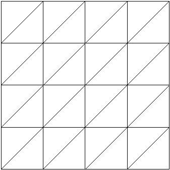
(a)

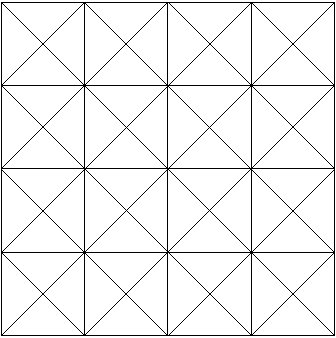
(b)

Figure 2. Diagonal mesh $\mathcal{M}_{N}^{D}$ (left) and crisscross mesh $\mathcal{M}_{N}^{C}$ (right) with $N=2$.

4.1. Smooth exact solution

We first consider a test case with smooth exact solution, namely

$$u(x_{1},x_{2})=\operatorname{curl}(x_{1}^{2}(1-x_{1})^{2}x_{2}^{2}(1-x_{2})^{2})\qquad p(x_{1},x_{2})=(x_{1}-0.5)(x_{2}-0.5).$$

We use the crisscross meshes $\mathcal{M}^{C}_{N}$ with $N\in\{0,1,\dots 8\}$ and the penalty parameter

$$\eta=6.$$

We report some values of the velocity error $\|u-u_{\mathrm{dG}}\|_{\mathrm{dG}}$ and of the pressure error $\|p-p_{\mathrm{dG}}\|_{L^{2}(\Omega)}$, for the three discretizations listed above, in Tables 1 and 2, respectively. For each sequence of errors $(e_{N})$, we compute the experimental order of convergence

$$\mathrm{EOC}_{N}:=\frac{\log(e_{N}/e_{N-1})}{\log(\#\mathcal{M}_{N-1}^{C}/\#\mathcal{M}_{N}^{C})},\qquad N\geq 1$$

where $\#\mathcal{M}_{N}^{C}$ denotes the number of triangles in $\mathcal{M}_{N}^{C}$. Observing the numerical data, we see that the errors of the three discretizations behave quite similarly and converge to zero at the maximum decay rate $(\#\mathcal{M}_{N}^{C})^{-0.5}$. In this case, the standard discretization should be preferred for the easier construction of the operator $E_{\mathrm{dG}}$.

N	$\mathtt{stnd}$	EOC	$\mathtt{qopt}$	EOC	$\mathtt{prob}$	EOC
4	8.2516e-03		8.3795e-03		8.5337e-03
5	3.8937e-03	0.54	3.9344e-03	0.55	4.1273e-03	0.52
6	1.8797e-03	0.53	1.8910e-03	0.53	2.0231e-03	0.51
7	9.2180e-04	0.51	9.2477e-04	0.52	1.0007e-03	0.51
8	4.5621e-04	0.51	4.5698e-04	0.51	4.9756e-04	0.50

Table 1. Section 4.1. Velocity errors of the standard ($\mathtt{stnd}$), quasi-optimal ($\mathtt{qopt}$) and quasi-optimal and pressure robust ($\mathtt{prob}$) discretizations with experimental orders of convergence.

N	$\mathtt{stnd}$	EOC	$\mathtt{qopt}$	EOC	$\mathtt{prob}$	EOC
4	4.4477e-03		4.4862e-03		4.3843e-03
5	2.2248e-03	0.50	2.2377e-03	0.50	2.2109e-03	0.49
6	1.1142e-03	0.50	1.1178e-03	0.50	1.1109e-03	0.50
7	5.5781e-04	0.50	5.5878e-04	0.50	5.5692e-04	0.50
8	2.7912e-04	0.50	2.7937e-04	0.50	2.7884e-04	0.50

Table 2. Section 4.1. Pressure errors of the standard ($\mathtt{stnd}$), quasi-optimal ($\mathtt{qopt}$) and quasi-optimal and pressure robust ($\mathtt{prob}$) discretizations with experimental orders of convergence.

4.2. Jumping pressure

In order to investigate the pressure robustness of the three discretizations, we consider a test case with smooth exact velocity and rough exact pressure, namely

$$u(x_{1},x_{2})=\operatorname{curl}\left(\>x_{1}^{2}(x_{1}-1)^{2}x_{2}^{2}(x_{2}-1)^{2}\>\right),\quad p(x_{1},x_{2})=\begin{cases}\frac{\pi}{\pi-1}&\text{if}\;\;x_{1}>\pi^{-1}\\ -\pi&\text{if}\;\;x_{1}<\pi^{-1}\end{cases}.$$

As before, we use the crisscross meshes $\mathcal{M}^{C}_{N}$ with $N\in\{0,1,\dots,8\}$ and the penalty parameter $\eta=6$. Note that the meshes do not resolve the discontinuity of $p$ along the line $x_{1}=\pi^{-1}$.

The data displayed in Figure 3 show that the velocity error of the quasi-optimal and pressure robust discretization fully exploits the regularity of $u$ and converges to zero at the maximum decay rate $(\#\mathcal{M}^{C}_{N})^{-0.5}$, in accordance with Theorem 19. In contrast, the low regularity of $p$ impairs the approximation of $u$ in the standard discretization and in the quasi-optimal one. In fact, the corresponding velocity errors converge at the suboptimal decay rate $(\#\mathcal{M}^{C}_{N})^{-0.25}$. This confirms, in particular, that the first estimate in Theorem 20 captures the correct behavior of the velocity error in the quasi-optimal discretization.

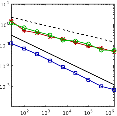
Figure 3. Section 4.2. Velocity error as a function of $\#\mathcal{M}^{C}_{N}$ for the standard ($\circ$), quasi-optimal ($*$) and quasi-optimal and pressure robust ($\square$) discretizations. Plain and dashed lines indicate the decay rates $(\#\mathcal{M}^{C}_{N})^{-0.5}$ and $(\#\mathcal{M}^{C}_{N})^{-0.25}$, respectively.

4.3. Locking

Finally, we investigate the robustness of the three discretizations with respect to the penalty parameter $\eta$. To this end, we consider the same exact solution as in section 4.1, with

$$\eta\in\{10,100,1000\}.$$

For a fair comparison, we measure the velocity errors in the parameter-independent norm

$$\|\cdot\|^{2}_{\mathrm{dG},1}:=\|\operatorname{\nabla_{\mathcal{M}}}\cdot\|_{L^{2}(\Omega)}^{2}+\int_{\Sigma}\dfrac{1}{h}\left\lvert\left\llbracket\cdot\right\rrbracket\right\rvert^{2}.$$

Note that $\|\cdot\|_{\mathrm{dG},1}\leq\|\cdot\|_{\mathrm{dG}}$ for the considered values of $\eta$. Since the three discretizations produce qualitatively similar results, we pick the quasi-optimal and pressure robust discretization as representative of the others.

We discretize the domain by the diagonal meshes $\mathcal{M}^{D}_{N}$ with $N\in\{0,1,\dots,7\}$. This choice is motivated by the fact that the constant $\delta_{\mathrm{SV}}$ from (26) is proportional to $(\mathcal{M}_{N}^{D})^{0.5}$ as a consequence of $Z_{\mathrm{SV}}=\{0\}$, see [7, equation 11.3.8]. Hence, according to the discussion in section 2.7, we expect to observe locking. The results displayed in Figure 4 confirm our expectation. In particular, we observe that the pressure error is more sensitive to the size of $\eta$ than the velocity error, in accordance with the estimates in Theorem 19.

One way to achieve robustness consists in weakening the jump penalization in the form $a_{\mathrm{dG}}$, as suggested in (27). With this modification, the results are almost insensitive to the size of $\eta$. Still, it has to be said that we obtain larger velocity errors than before for moderate values of $\eta$.

(a)

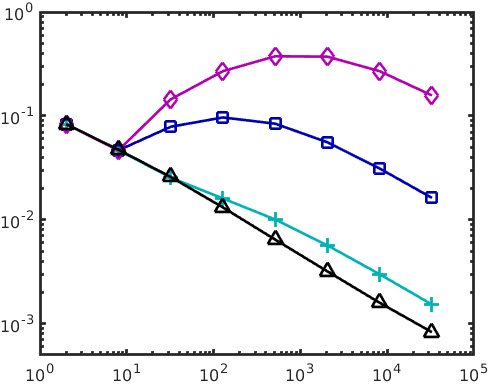
(b)

Figure 4. Section 4.3. Velocity (left) and pressure (right) errors of the quasi-optimal and pressure robust discretization as functions of $\#\mathcal{M}_{N}^{D}$ for $\eta=10$ ($+$), $\eta=100$ ($\square$) and $\eta=1000$ ($\lozenge$). The variant with weak jump penalization is also considered ($\triangle$) and the results for the three values of $\eta$ graphically coincide.

Funding

Christian Kreuzer gratefully acknowledges partial support by the DFG research grant “Convergence Analysis for Adaptive Discontinuous Galerkin Methods” (KR 3984/5-1). The research of Pietro Zanotti was supported by the GNCS-INdAM through the program “Finanziamento giovani ricercatori 2019-2020”.

References

- [1] D. N. Arnold, F. Brezzi, B. Cockburn, and L. D. Marini, Unified analysis of discontinuous Galerkin methods for elliptic problems, SIAM J. Numer. Anal., 39 (2001/02), pp. 1749–1779.
- [2] I. Babuška and M. Suri, On locking and robustness in the finite element method, SIAM J. Numer. Anal., 29 (1992), pp. 1261–1293.
- [3] I. Babuška and M. Suri, Locking effects in the finite element approximation of elasticity problems, Numer. Math., 62 (1992), pp. 439–463.
- [4] S. Badia, R. Codina, T. Gudi, and J. Guzmán, Error analysis of discontinuous Galerkin methods for the Stokes problem under minimal regularity, IMA J. Numer. Anal., 34 (2014), pp. 800–819.
- [5] Á. Baran and G. Stoyan, Gauss-Legendre elements: a stable, higher order non-conforming finite element family, Computing, 79 (2007), pp. 1–21.
- [6] D. Boffi, F. Brezzi, and M. Fortin, Mixed Finite Element Methods and Applications, vol. 44 of Springer Series in Computational Mathematics, Springer, Heidelberg, 2013.
- [7] S. C. Brenner and L. R. Scott, The Mathematical Theory of Finite Element Methods, vol. 15 of Texts in Applied Mathematics, Springer, New York, third ed., 2008.
- [8] H. Brezis, Functional Analysis, Sobolev Spaces and Partial Differential Equations, Universitext, Springer, New York, 2011.
- [9] B. Cockburn, G. Kanschat, and D. Schötzau, A note on discontinuous Galerkin divergence-free solutions of the Navier-Stokes equations, J. Sci. Comput., 31 (2007), pp. 61–73.
- [10] M. Crouzeix and R. S. Falk, Nonconforming finite elements for the Stokes problem, Math. Comp., 52 (1989), pp. 437–456.
- [11] M. Crouzeix and P.-A. Raviart, Conforming and nonconforming finite element methods for solving the stationary Stokes equations. I, Rev. Française Automat. Informat. Recherche Opérationnelle Sér. Rouge, 7 (1973), pp. 33–75.
- [12] D. A. Di Pietro and A. Ern, Mathematical Aspects of Discontinuous Galerkin Methods, vol. 69 of Mathématiques & Applications (Berlin) [Mathematics & Applications], Springer, Heidelberg, 2012.
- [13] A. Ern and J.-L. Guermond, Theory and practice of finite elements, vol. 159 of Applied Mathematical Sciences, Springer-Verlag, New York, 2004.
- [14] J. Guzmán and M. Neilan, Inf-sup stable finite elements on barycentric refinements producing divergence–free approximations in arbitrary dimensions, SIAM J. Numer. Anal., 56 (2018), pp. 2826–2844.
- [15] P. Hansbo and M. G. Larson, Discontinuous Galerkin methods for incompressible and nearly incompressible elasticity by Nitsche’s method, Comput. Methods Appl. Mech. Engrg., 191 (2002), pp. 1895–1908.
- [16] C.-J. Heine, D. Köster, O. Kriessl, A. Schmidt, and K. Siebert, ALBERTA: an adaptive hierarchical finite element toolbox. accessed , http://www.alberta-fem.de.
- [17] V. John, A. Linke, C. Merdon, M. Neilan, and L. G. Rebholz, On the divergence constraint in mixed finite element methods for incompressible flows, SIAM Rev., 59 (2017), pp. 492–544.
- [18] C. Kreuzer and P. Zanotti, Quasi-optimal and pressure robust discretizations of the Stokes equations by new augmented Lagrangian formulations. arXiv:1902.03313, 2019.
- [19] A. Linke, On the role of the Helmholtz decomposition in mixed methods for incompressible flows and a new variational crime, Comput. Methods Appl. Mech. Engrg., 268 (2014), pp. 782–800.
- [20] R. H. Nochetto and J.-H. Pyo, Optimal relaxation parameter for the Uzawa method, Numer. Math., 98 (2004), pp. 695–702.
- [21] A. Schmidt and K. G. Siebert, Design of adaptive finite element software, vol. 42 of Lecture Notes in Computational Science and Engineering, Springer-Verlag, Berlin, 2005.
- [22] L. R. Scott and M. Vogelius, Norm estimates for a maximal right inverse of the divergence operator in spaces of piecewise polynomials, RAIRO Modél. Math. Anal. Numér., 19 (1985), pp. 111–143.
- [23] A. Toselli, discontinuous Galerkin approximations for the Stokes problem, Math. Models Methods Appl. Sci., 12 (2002), pp. 1565–1597.
- [24] A. Veeser, Approximating gradients with continuous piecewise polynomial functions, Found. Comput. Math., 16 (2016), pp. 723–750.
- [25] A. Veeser and P. Zanotti, Quasi-optimal nonconforming methods for symmetric elliptic problems. I—Abstract theory, SIAM J. Numer. Anal., 56 (2018), pp. 1621–1642.
- [26] A. Veeser and P. Zanotti, Quasi-optimal nonconforming methods for symmetric elliptic problems. III—Discontinuous Galerkin and other interior penalty methods, SIAM J. Numer. Anal., 56 (2018), pp. 2871–2894.
- [27] R. Verfürth and P. Zanotti, A quasi-optimal Crouzeix–Raviart discretization of the Stokes equations, SIAM J. Numer. Anal., 57 (2019), pp. 1082–1099.