A class of quasi-eternal non-Markovian Pauli channels and their measure
Abstract
We study a class of qubit non-Markovian general Pauli dynamical maps with multiple singularities in the generator. We discuss a few easy examples involving trigonometric or other non-monotonic time dependence of the map, and discuss in detail the structure of channels which don’t have any trigonometric functional dependence. We demystify the concept of a singularity here, showing that it corresponds to a point where the dynamics can be regular but the map is momentarily non-invertible, and this gives a basic guideline to construct such non-invertible non-Markovian channels. Most members of the channels in the considered family are quasi-eternally non-Markovian (QENM), which is a broader class of non-Markovian channels than the eternal non-Markovian channels. In specific, the measure of quasi-eternal non-Markovian (QENM) channels in the considered class is shown to be in the isotropic case, and about 0.96 in the anisotropic case.
I Introduction
It is well known that noise is an inevitable attendant feature of quantum systems in a realistic scenario Reich et al. (2015); Liu et al. (2011); Chruściński and Kossakowski (2010). Quantum non-Markovianity is a memory property that can help the system recover coherence through environment-induced decoherence Breuer and Petruccione (2002); Banerjee (2018). In that sense, it can be thought of as a resource for an efficient real-life implementation of quantum information processing tasks B. Bylicka and Maniscalco (2014), such as quantum key distribution Utagi et al. (2020a); Thapliyal et al. (2017), quantum teleportation of mixed quantum states E.M. Laine (2014), and quantum thermodynamics Thomas et al. (2018), to name a few. Therefore, the characterization and study of non-Markovian quantum channels continues to be a major research activity Li et al. (2019); Naikoo et al. (2019a); Naikoo and Banerjee ; Naikoo et al. (2019b); Utagi et al. (2020b).
In many of the works in the literature, the study of non-Markovian dynamics has been done by incorporating physical models of particular interest Grabert et al. (1988); Banerjee and Ghosh (2000, 2003); Kumar et al. (2018). Here, we provide a model-independent framework, introduced in Shrikant et al. (2018), in which a method of creating non-Markovian analogues of dephasing and depolarizing channels was presented. We adopt that method to obtain a family of general Pauli dynamical maps, which it will be convenient to split into the two classes– of the isotropic and anisotropic non-Markovian depolarizing channels, which are the special instances of generalized Pauli channels, which in turn are special cases of random unitary channels. The method is tailored so that the non-Markovianity is associated with the presence of singularities in the time-local generator. Often it will be convenient to simplify the description of the decoherence using a noise parameter instead of time itself Shrikant et al. (2018), whose functional form is not needed for the purpose of this paper. For example, in the dephasing channel given by , corresponds to . Throughout this paper, we associate time-dependence of states, operators and functions with .
The appearance of singularities in the time-local generator is not new. Phenomenological models such as a two-level system interacting with a bosonic reservoir Breuer and Petruccione (2002) constitute an example of an instance in which the time-local generator in the canonical master equation has infinite singularities.
This paper is arranged as follows. In Section II we review non-Markovianity conditions for generalized Pauli channels and dwell briefly on the existence of singularities. In Section III, we give a few easy examples of channels that have an infinite number of singularities, in order to motivate the non-trivial character of the channels introduced in the next section. In Section IV, we present depolarizing channel with anisotropic non-Markovianity as an example of a generalized Pauli channel, which in turn is a special case of random unitary dynamics. An analysis of the singularities in the master equation of the channel is presented in Section V, along with a demonstration of the fact that these singularities are non-pathological. In Section VI we revisit the isotropic version of the non-Markovian depolarization channel, and quantify its non-Markovianity using a measure due to Hall-Cresser-Li-Anderson (HCLA) Hall et al. (2014), as well as a recently introduced Utagi et al. (2020b) measure. In Section VII we show that most of the channels studied here are quasi-eternally non-Markovian (QENM), i.e., they have negative decoherence rate after a finite time (which corresponds to a singularity), but may be completely positive (CP)-divisible before that De Santis et al. (2019). Then we conclude in Section VIII. A list of notations used is summarized in the Table in Appendix B.
II Non-Markovianity conditions for Pauli dynamical maps
A generalized Pauli channel Chruscinski and Wudarski (2013) is given by the operator-sum (or, Kraus) representation with being the Kraus operators, where and are Pauli and operators, respectively. By projecting the map onto the Pauli matrices, we obtain the operator eigenvalue equation , where are the time-dependent eigenfunctions of the Pauli map given by
| (1) |
and
| (6) |
is the Hadamard matrix. The decay rates are generally obtained as Chruscinski and Wudarski (2013)
| (7) |
Assuming that intermediate maps for all , are invertible, the canonical form of master equation corresponding to the map (13) is
| (8) |
where is the decoherence rate corresponding to the unitary operation in the channel. is the generator of the dynamics such that .
Assuming that the channel is invertible, the necessary condition for it to be completely positive CP-divisible Rivas et al. (2010) is:
| (9) |
i.e., the positivity of Lindblad rates that appear in the time-local Gorini-Kossakowski-Lindblad-Sudarshan (GKSL) form such as Eq. (8). A necessary condition for positive P-divisibility (or equivalently of Markovianity according to the criterion due to Breuer-Laine-Piilo (BLP) Breuer et al. (2009), in the qubit case) is Chruscinski and Wudarski (2013)
| (10) |
However, if the channel is non-invertible, as in the present case, then the condition Eq. (9) is only sufficient but not necessary for CP-divisibility Chruściński et al. (2018). Specifically, the rate may be temporarily negative after a singularity even though the channel is CP-divisible.
Note that at the point of singularity in the time-local generator, the rates in the GKSL equation become infinite and the map is momentarily non-invertible. In the present case, these singularities are finite in number and non-pathological Shrikant et al. (2018), and the above criteria can be applied at all points except these.
From Eqs. (9) and (10), we find that P-indivisibility implies CP-indivisibility, but not vice versa. The conditions under which these two criteria are equivalent is investigated in Ref. Chruściński et al. (2018).
From Eq. (7) it follows that a generator possesses a singularity whenever . Later we will show that if in finite time , then the decay rate flips sign, thereby giving rise to non-Markovian evolution following the singularity at the time .
Significantly, we shall point out that the singularities are non-pathological Shrikant et al. (2018); Jagadish et al. (2019), in that the dynamics can be regular at the instant of singularity . In fact, the existence of such a singularity in the generator corresponds to a momentary indistinguishability of the evolved version of distinct states in the sense of BLP Breuer et al. (2009), and thereby the momentary non-invertibility of the dynamical map in the sense of CP-divisibility according to the Rivas-Huelga-Plenio (RHP) criterion Rivas et al. (2010). For purposes of quantification, the singularities may be suitably normalized.
For any qubit Pauli map with multiple decoherence rates, it was shown Chakraborty and Chruściński (2019) that non-Markovianity criterion based on distinguishability and CP-divisibility are equivalent. Therefore, we associate the non-Markovianity of channels in this work with the negativity of one or more decay rates in the canonical master equation.
III Elementary examples of non-Markovian Pauli channels with singularities
In this section we show how one can straightforwardly obtain an infinite number of singularities in the generator with oscillatory channel decay probabilities. As a quick example, consider a dephasing channel with Kraus operators:
| (11) |
where . Here, is the identity operator and is Pauli Z operator. A singularity corresponds to the point of maximal dephasing, which collapses all states on the same azimuth of the Bloch sphere. The decay rate of the channel reads , which has infinite singularities, corresponding to time being odd multiples of . As a second easy example, consider a Pauli channel with the Kraus operators:
| (12) |
Singularities correspond, as above, to times where vanishes, leading to maximal mixing, and hence momentary irreversibility. The above maps have time-dependent eigenvalues , and the decay rates (7) are found to be .
The concept of eternal non-Markovianity was introduced in Hall et al. (2014), where a Pauli channel with decay rates and was proposed as an example of a CP-indivisible channel that is Markovian according to the distinguishability criterion Breuer et al. (2009). As evident, this channel has the property that it has a negative rate for all times , and accordingly called “eternally non-Markovian”.
Following the definition proposed in De Santis et al. (2019), we shall refer to a channel as “quasi-eternally non-Markovian” (QENM) if there exists a finite time such that is CP-indivisible for all times , i.e., if there exists a finite such that the channel is CP-indivisible for all . The channel may be CP-divisible for . We remark that this differs from the notion of quasi-eternal non-Markovianity proposed in Ref. Rivas (2017), where this term refers to a dynamics that is CP-indivisible for time , and is the instant at which the system has almost reached its steady state.
In Eq. (11), setting , we find that this function gives an easy example of a dephasing channel that is quasi-eternally non-Markovian (QENM), with the rate , attaining a singularity at the point where . The rate is positive before the singularity and negative after it.
The above examples are manifestly maps that are non-monotonic, in that the mixing functions such as are non-monotonic. This is in consonance with the usual notion of associating non-Markovian behavior with break in monotonicity. However, in this work, we will discuss a class of completely positive trace preserving (CPTP) Pauli dynamical maps that are monotonic. Specifically, this entails that time-dependent eigenvalues are monotonic functions. The origin of non-Markovianity here is that the maps evolve the state beyond the point of maximum decoherence, leading to negative decay rates. The maps so produced are naturally quasi-eternal non-Markovian (QENM) in the sense mentioned above.
IV Anisotropic non-Markovian depolarization
In the following, we adopt the framework of Shrikant et al. (2018), where non-Markovian analogues of Pauli dephasing and depolarizing channels were introduced. Here, in terms of the parameter , the map of a qubit Pauli channel is given by:
| (13) |
where , and are Pauli operators, and . Henceforth, it will be convenient to use the notation where a monotonic parameter is used in place of time . This is done essentially because the detailed functional form of does not affect the results here.
Using the method introduced in Shrikant et al. (2018), one may generate non-Markovian extensions of Kraus operators ’s as:
| (14) |
where () is a real function, and is a real parameter, which acts like time, in this framework. It rises monotonically from 0 to , and its functional form does not matter here. The variables satisfy the following condition
| (15) |
as a consequence of the completeness requirement . Moreover, the channel is ensured to be completely positive in the sense that the Choi matrix is positive semidefinite i.e., for all , where is a maximally entangled state. And the channel is said to be CP-divisible if the Choi matrix of the intermediate map for all is positive, which will be discussed in Section (V.3). In agreement with Eq. (15), we make the following choices: , , and , where are real. Then, the non-Markovian Kraus operators take the form
| (16) |
The parameters may be seen to represent the non-Markovian behavior of the channel, such that setting reduces the Kraus operators in Eq. (16) to those in the conventional Markovian depolarizing channel, which is a type of Pauli channel. It is easy to see that setting reduces (16) to the (isotropic) non-Markovian depolarizing channel introduced in Shrikant et al. (2018).
By definition, , which implies that . In a depolarizing channel, the mixing parameter varies from to , at which point the state becomes maximally mixed. For , the system deviates from , i.e., to re-cohere.
The canonical decay rates in the equation (8) are calculated using the method given in (Chruscinski and Wudarski, 2013, Section 2), and are found to be:
| (17) |
where
| (18a) | ||||
| (18b) | ||||
where . Here and .
V Analysis of singularities
We now consider the questions of how the non-Markovian parameters and determine the location of the singularities and thereby the nature of the intermediate map, and finally the physical interpretation of the singularities.
V.1 Location of singularities
In order to analyze the singularities, one needs to extract the roots of Eq. (18). The zeros of in Eq. (17) yield the singularities of the decay rates. Solving for any , one finds:
| (19) |
are the two solutions for in the second equation of Eq. (18) for a given . The larger of the two roots can be ignored as it appears after . Here, corresponds to Markovian evolution, and if any one of the parameter is non-zero, the channel exhibits non-Markovian evolution after it experiences a singularity.
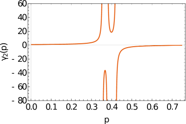
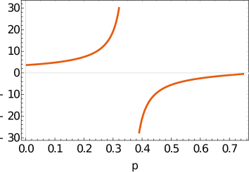
The singularity pattern in Figure 1 can be understood by following the behavior of any function in Eqs. (17). This immediately shows that the function flips its sign at . An example is plotted in Figure (2).
Referring to the form of Eq. (17), this implies that each rate by itself will have its sign flipped at the singularities. To see this, assuming more than one singularity, note that close to one of the singularities, only the function(s) that diverges at that singularity will be unbounded, whereas the other contribution(s) to the given rate will be finite. Thus, the rate as a whole inherits the sign flipping behavior. Figure 1 exemplifies this pattern. Here the behavior of the decay rate of is the composite of the above pattern of evolution of the three terms .
If , then , leading to three singularities, whilst if two of the non-Markovianity parameters are equal, say , with , then there are two singularities at and at . If , then a single singularity occurs at .
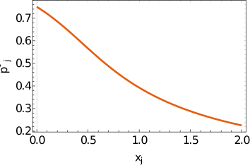
The function monotonically falls with , which varies in the interval (Figure 3). In particular
showing that as the non-Markovianity parameters or are increased, the position of any singularity here shifts monotonically to the left.
V.2 (Not) complete positivity of the intermediate map
In light of Ref. Chruściński et al. (2018), negativity of a decoherence rate in a time interval following the first singularity will not necessarily imply CP-indivisibility. Therefore, to establish that the map is CP-indivisible in this region, we require to explicitly consider an intermediate map that should be not completely positive (NCP) and, in particular, that at least one of the eigenvalues of the Choi matrix of the intermediate map is negative. A specific instance of this is given in Figure (4), as discussed below.
A completely positive (CP) trace preserving map taking the quantum state from time to may generally be written as , where the intermediate map need not be CP. Assuming that the intermediate map is invertible, we have . The time-dependent eigenvalues of the Choi matrix are given below: Let , with Then
| (20) |
where, and , for all . Here, , with are as given in Eq. (19). The eigenvalues are plotted against time for a fixed in Figure (4). It can be shown that the decay rates obtained by Eq.(7) flip sign from negative to positive or vice versa at each singularity. An example of this behavior was discussed in the previous section, with respect to rate , which flips sign from positive to negative at the singular point (see in Fig. (1)). Similarly, it can be shown that become increasingly negative as the singularity at is approached, and flips sign to positive at the singularity, indicating the onset of CP-indivisibility prior to the singularity. This explains the negativity of the bold-red curve in the Fig. (4) before the singularity at . This example brings out an interesting interplay between singularities, negativity of decay rates and CP-indivisibility in Pauli channels.

V.3 Singularities are not pathological
An important point that was implicit earlier, and which we make explicit now, is that although the generator in the GKSL equation has a singularity, yet the dynamics is regular. The singularity corresponds on the level of the map to a momentary indistinguishability of a family of initial states, and thus to the non-invertibility of the map, i.e., the momentary non-existence of , after which a recurrence occurs. Noting that generator is the dynamical map’s logarithmic derivative, i.e., , the singular nature of the generator may be understood as a consequence of the non-invertibility of the map, despite the latter’s differentiability.
This can be verified easily in the case of the isotropic non-Markovian depolarizing channel mentioned above, by noting that the trace distance (TD) between two initial pair of states under our channels fall monotonically continuously for =0. On the other hand, for , in the case of the isotropic depolarizing channel, at the point of singularity, given by (Eq. (30)), TD vanishes, after which they again increase. However, the time evolution of TD is continuous even at , and in that sense, the singularity is not pathological.
We illustrate this aspect with the following mathematical arguments. The final state obtained after the channel acts on a generic state:
| (26) |
where
| (27) | ||||
| (28) |
Substituting from Eq. (30) in Eq. (28), we find that the state obtained is the maximally mixed state, meaning that all initial states (irrespective of the parameters and ) become indistinguishable at this point momentarily, and the map is non-invertible at that point. Specifically, at from Eq. (18b) we find that all vanish; noting that , it can be seen that vanishing corresponds to the non-invertibility of .
But this singularity is not pathological in the sense that the dynamics itself remains regular, even through the singular point. In particular, the map is differentiable, in that and from Eq. (18a) we find that is differentiable throughout the interval . Moreover, this is consistent with the fact that for , the states Eq. (LABEL:eq:stateisotropic) are distinguishable, and thus the map is invertible.
VI Quantifying non-Markovianity: the isotropic case
The basic dependence of the degree of non-Markovianity of the above channels on the parameters and can be studied more easily by considering the isotropic case, determined by the single non-Markovian parameter . In particular, we shall study the Hall-Cresser-Li-Andersson (HCLA) measure Hall et al. (2014) and the so-called SSS measure, recently introduced in Ref. Utagi et al. (2020b).
In this case, all the decay rates , and are equal and given by:
| (29) |
In view of Eq. (17), Eq. (19) correspondingly reduces to
| (30) |
Here is the single singularity that occurs in elements of this family of channels.
The form of Eq. (29) shows that, as with the anisotropic case, the sign of the decay rate discontinuously flips from positive to negative at , after which it continuously decreases in magnitude. However, whether this eventually leads to a positive rate depends on the specific value of , as discussed below. In particular, note that in Eq. (29), the denominator remains negative for . On the other hand, the numerator monotonically falls with . If is large enough to make the numerator negative, then for such sufficiently large values, the asymptotic rate becomes positive. This is determined as follows. The point at which the numerator vanishes is
| (31) |
Thus, the range of for which would correspond to the failure of the QENM condition. Observe that , and corresponds to . Therefore, the range corresponds to the failure of the QENM condition. In Figure 2, would correspond to the point where the rising (i.e., second) curve meets the line. If , then the channel decay rate becomes positive asymptotically.
Recently, Ref. Utagi et al. (2020b) introduced a measure (which may be called the SSS measure for convenience) of non-Markovianity based on the deviation of the generator of a map giving rise to a quantum dynamical semigroup (QDS) structure. This measure expresses the idea that QDS form is equivalent to the notion of memorylessness wherein the form of the dynamical map remains invariant in time over the evolution, and captures a notion of Markovianity stronger than CP-divisibility. The intermediate infinitesimal map is given by Let represent the map representing semigroup evolution. Then the distance between two intermediate infinitesimal maps is: , where is the generator of the dynamics and that pertaining to the semigroup form (which is time-independent). The required weaker-than-CP-divisible measure is based on the deviation from the semigroup form:
| (32) |
where is the trace norm of a matrix , and is the Choi matrix corresponding to operator . For the channel (16), with , where , the measure (32) reads,
| (33) |
where is given by the Eq. (29), and is the constant decay rate obtained when , which pertains to semigroup dynamics. In practice, it may be convenient to use the family semigroup limit value of , which is found to be , given that the parametrization of time takes the form , where is a real number defining the strength of decay.
In Ref. Utagi et al. (2020b), the quantification Eq. (32) does not explicitly consider the occurrence of singularities. Here, we point that the quantification can be straightforwardly extended to the latter case, such as in the present work, by replacing the rate with a suitable re-normalized value. Here we use .
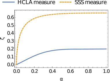
Furthermore, the resulting measure (33) itself can be suitably normalized as to confine it to the range . The doubly renormalized weak non-Markovianity measure against is plotted as the dashed line in Fig. (5), depicting a monotonic increase of the measure with .
The renormalization technique adopted therefore serves the purpose not only to tame the singularity, but also to ensure that the non-Markovianity measure within a given family of non-Markovian channels lies between 0 (the Markovian limit in the sense of Ref. Utagi et al. (2020b)) and 1 (the maximally non-Markovian in the family).
The non-Markovian behavior of this family of channels can be physically understood as follows. From Eq. (16), we find that (more generally, or ) represents the degree by which the channel governed by a monotonic decoherence function overshoots the point of maximal decoherence, and thus corresponds to a region of recurrence. This stands in contrast to the type of non-Markovianity channels we presented as elementary examples in section III, where memory effects are incorporated easily by employing non-monotonic functions in the decoherence parameter . As is increased, the channel’s overshoot is greater, and correspondingly the greater is the non-Markovianity, as reflected in Fig. (5).
A point worth mentioning here is that the above measure yields a non-vanishing value even for CP-divisible channels that deviate from the semigroup structure, as discussed in Ref. Utagi et al. (2020b). Furthermore, the main trend captured above, that of non-Markovianity increasing monotonically as a function of the parameter , is also reflected in the HCLA measure, depicted by the solid curve in Fig. (5).
The non-Markovianity of a channel in this family according to the measure of Hall et al. (2014) is:
| (34) | ||||
| (38) |
where, is the normalized version of in the time-local master equation.
For example, consider the case of , for which the lone singularity is , after which the decay rate is negative. Note that the rate has the same behavior as the ratio function depicted in Figure 2. The non-Markovianity measure corresponding to the two expressions in Eq. (38) are, respectively
| (39a) | ||||
| (39b) | ||||
Here and . Note the expression is continuous at . The corresponding plot of in the Eq. (39a & 39b) is given as the bold (blue) curve in Figure (5) and depicts, as expected, that the degree of non-Markovianity is an increasing function of .
VII Volume of quasi-eternal non-Markovian Pauli channels
For the family of channels considered here, the QENM property can be checked by verifying that for any . In the case of isotropically non-Markovian depolarizing channel (setting ), for , as discussed earlier, the channel is CP-divisible for and CP-indivisible for , defined in Eq. (31). Since precisely for the set , the measure of isotropic NM depolarizing channels that is QENM is .
In the general anisotropic case, it follows from Eq. (17) that the conditions for and to be negative at is
| (40a) | ||||
| (40b) | ||||
| (40c) | ||||
respectively, where , and . For a channel characterized by a specific value and , if any one of the conditions (40) is satisfied, then then channel would be QENM. The volume (per Euclidean measure) of the set of QENM channels is that Eq. (40a) or Eq. (40b) or Eq. (40c) holds. In the parameter space of and , it is about 0.955.
Also, it would be pertinent to point out that the the channel introduced and characterized in Shrikant et al. (2018) is quasi-eternal non-Markovian. This is reviewed in the Appendix, where it is characterized in terms of physical time instead of the formal parameter .
VIII Conclusions
This paper introduces depolarizing channels that are anisotropically non-Markovian, generalizing a previously proposed method Shrikant et al. (2018). These channels are characterized by up to three singularities in the generator. The three canonical decoherence rates were shown to flip sign after each singularity. Most members of the channels in the family are quasi-eternally non-Markovian (QENM), which is a broader class of non-Markovian channels than the eternal non-Markovian channels. The measure of QENM channels is found to be in the isotropic case, and 0.96 in the anisotropic case. This highlights a physical attribute to the isotropic and anisotropic non-Markovian depolarizing channels.
Possible future directions would be to generalize this approach to random unitary channels, and study their singularity pattern and QENM property. Importantly, physical systems that can realize this, or even the simpler non-Markovian dephasing channels, would be of practical interest. Such maps show an interesting feature of level crossing eigenvalues, about which we discussed in depth in Ref. Shrikant et al. (2018). This may offer a clue about the kind of systems that may demonstrate such non-Markovian behavior in Nature. Reservoir engineering has recently witnessed good advances in various platforms for practical quantum information processing, and this provides a potential avenue to explore in this context.
Acknowledgements.
SU and VNR thank Admar Mutt Education Foundation for the scholarship. RS and SB acknowledge, respectively, the support from Interdisciplinary Cyber Physical Systems (ICPS) program of the Department of Science and Technology (DST), India, Grants No.: DST/ICPS/QuEST/Theme-1/2019/14 and DST/ICPS/QuEST/Theme-1/2019/6. RS also acknowledges the support of the Govt. of India DST/SERB grant MTR/2019/001516.References
- Reich et al. (2015) D. M. Reich, N. Katz, and C. P. Koch, Scientific reports 5, 12430 (2015).
- Liu et al. (2011) B.-H. Liu, L. Li, Y.-F. Huang, C.-F. Li, G.-C. Guo, E.-M. Laine, H.-P. Breuer, and J. Piilo, Nature Physics 7, 931 (2011).
- Chruściński and Kossakowski (2010) D. Chruściński and A. Kossakowski, Physical review letters 104, 070406 (2010).
- Breuer and Petruccione (2002) H.-P. Breuer and F. Petruccione, The theory of open quantum systems (Oxford University Press, 2002).
- Banerjee (2018) S. Banerjee, Open quantum systems (Springer Nature Singapore Pte Ltd., 2018).
- B. Bylicka and Maniscalco (2014) D. C. B. Bylicka and S. Maniscalco, Scientific Reports 4 (2014).
- Utagi et al. (2020a) S. Utagi, R. Srikanth, and S. Banerjee, Quantum Information Processing 19, 366 (2020a).
- Thapliyal et al. (2017) K. Thapliyal, A. Pathak, and S. Banerjee, Quantum Information Processing 16, 115 (2017).
- E.M. Laine (2014) J. P. E.M. Laine, H.P. Breuer, Scientific Reports 4 (2014).
- Thomas et al. (2018) G. Thomas, N. Siddharth, S. Banerjee, and S. Ghosh, Phys. Rev. E 97, 062108 (2018), URL https://link.aps.org/doi/10.1103/PhysRevE.97.062108.
- Li et al. (2019) C.-F. Li, G.-C. Guo, and J. Piilo, EPL (Europhysics Letters) 127, 50001 (2019), URL https://doi.org/10.1209%2F0295-5075%2F127%2F50001.
- Naikoo et al. (2019a) J. Naikoo, S. Dutta, and S. Banerjee, Phys. Rev. A 99, 042128 (2019a), URL https://link.aps.org/doi/10.1103/PhysRevA.99.042128.
- (13) J. Naikoo and S. Banerjee, Quantum Inf Process p. 19: 29 (2020).
- Naikoo et al. (2019b) J. Naikoo, S. Banerjee, and R. Srikanth, arXiv:1911.07677 (2019b).
- Utagi et al. (2020b) S. Utagi, R. Srikanth, and S. Banerjee, Scientific Reports 10, 1 (2020b).
- Grabert et al. (1988) H. Grabert, P. Schramm, and G.-L. Ingold, Physics Reports 168, 115 (1988), ISSN 0370-1573, URL http://www.sciencedirect.com/science/article/pii/0370157388900233.
- Banerjee and Ghosh (2000) S. Banerjee and R. Ghosh, Phys. Rev. A 62, 042105 (2000), URL https://link.aps.org/doi/10.1103/PhysRevA.62.042105.
- Banerjee and Ghosh (2003) S. Banerjee and R. Ghosh, Phys. Rev. E 67, 056120 (2003), URL https://link.aps.org/doi/10.1103/PhysRevE.67.056120.
- Kumar et al. (2018) N. P. Kumar, S. Banerjee, R. Srikanth, V. Jagadish, and F. Petruccione, Open systems & Information Dynam 25, 1850014 (2018).
- Shrikant et al. (2018) U. Shrikant, R. Srikanth, and S. Banerjee, Phys. Rev. A 98, 032328 (2018), URL https://link.aps.org/doi/10.1103/PhysRevA.98.032328.
- Hall et al. (2014) M. J. W. Hall, J. D. Cresser, L. Li, and E. Andersson, Phys. Rev. A 89, 042120 (2014).
- De Santis et al. (2019) D. De Santis, M. Johansson, B. Bylicka, N. K. Bernardes, and A. Acín, arXiv:1903.12218 (2019).
- Chruscinski and Wudarski (2013) D. Chruscinski and F. A. Wudarski, Physics Letters A 377, 1425 (2013), ISSN 0375-9601, URL http://www.sciencedirect.com/science/article/pii/S0375960113003666.
- Rivas et al. (2010) Á. Rivas, S. F. Huelga, and M. B. Plenio, Phys. Rev. Lett 105, 050403 (2010).
- Breuer et al. (2009) H.-P. Breuer, E.-M. Laine, and J. Piilo, Phys. Rev. Lett 103, 210401 (2009).
- Chruściński et al. (2018) D. Chruściński, A. Rivas, and E. Størmer, Phys. Rev. Lett. 121, 080407 (2018), URL https://link.aps.org/doi/10.1103/PhysRevLett.121.080407.
- Jagadish et al. (2019) V. Jagadish, R. Srikanth, and F. Petruccione, Phys. Rev. A 100, 012336 (2019), URL https://link.aps.org/doi/10.1103/PhysRevA.100.012336.
- Chakraborty and Chruściński (2019) S. Chakraborty and D. Chruściński, Phys. Rev. A 99, 042105 (2019), URL https://link.aps.org/doi/10.1103/PhysRevA.99.042105.
- Rivas (2017) A. Rivas, Phys. Rev. A 95, 042104 (2017), URL https://link.aps.org/doi/10.1103/PhysRevA.95.042104.
Appendix
Appendix A Quasi-eternal non-Markovian dephasing
We consider a non-Markovian analog of dephasing presented and analyzed in Shrikant et al. (2018), whose Kraus representation of map reads
| (41) |
where is Pauli Z operator. is a real parameter that defines the degree of non-Markovianity of the channel and ranges from 0 to 1, and can be thought of as parametric time whose functional form may be given by such that when , and when , . The decay rate can be read out from the canonical master equation or simply from the effect of map (41) on a qubit density matrix as , with , for all . Therefore, for NMD of the form (41) we find the decay rate to be
| (42) |
In terms of actual physical time , the decay rate (42) becomes:
| (43) |
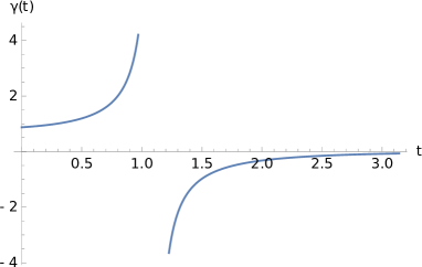
This is plotted against time in Fig. (6). It is interesting to note that when , then but never becomes zero. Hence, one may call it ‘quasi-eternally non-Markovian dephasing’ for the reason that the channel makes transition to being non-Markovian only after the critical transition time and remains so ever after, see Fig. (6). This critical time corresponds to a singularity in the time-local generator. Interestingly, the appearance of singularity in the generator is not trivial and may prompt one to look for some interesting physical features of dynamics with decay rate of the form (43), and finding such physical systems is a question we leave open.
The singularity in time at which the decay rate blows up is found to be . Correspondingly, at the map level, one finds a momentary non-invertibility of the intermediate map. The pair of real numbers , with defines a family of non-Markovian dephasing (NMD) channels with representing the quantum dynamical semigroup limit of the family, and . The reader is referred to Shrikant et al. (2018) for a detailed study of this channel.
Appendix B Appendix: Table of notations
| List of notations | |
|---|---|
| Symbol | Meaning |
| Quantum dynamical map | |
| Physical time | |
| Parametric time, which increases monotonically with time | |
| Eigenvalue of Pauli map corresponding to the eigenoperator given by Pauli | |
| Kraus operator | |
| Probability defined such that | |
| Angular frequency | |
| and | Non-Markovian parameters for the anisotropic depolarizing channel |
| Non-Markovian parameter for the isotropic depolarizing channel | |
| The point in time when singularities occur in the generator of isotropic depolarization | |
| The point in time when decay rate becomes positive in the generator of isotropic depolarization | |
| Time-independent Lindblad generator corresponding to semigroup evolution | |
| Time-dependent Lindblad generator | |
| The point in physical time when a singularity occurs in the generator | |
| or | Time-dependent decay rate |
| Time-independent decay rate or the rate in the semigroup limit | |
| Some real function of | |