Further Geometric and Lyapunov Characterizations of Incrementally Stable Systems on Finsler Manifolds

Abstract

In this paper, we report several new geometric and Lyapunov characterizations of incrementally stable systems on Finsler and Riemannian manifolds. A new and intrinsic proof of an important theorem in contraction analysis is given via the complete lift of the system. Based on this, two Lyapunov characterizations of incrementally stable systems are derived, namely, converse contraction theorems, and revelation of the connection between incremental stability and stability of an equilibrium point, in which the second result recovers and extends the classical Krasovskii’s method.

A technical mistake in Theorem 4 has been corrected in this version compared to the IEEE TAC version [1]. See the red texts.

1 Introduction and Motivation

Incremental stability, also termed as contraction in the literature, is concerned with the attractive behaviour of any pairs of trajectories of a system. This notion dates back to the 1950s and 1960s, known as extreme stability, which was introduced to study the stability of periodic orbits of dynamical systems [2, 3]; at the time, the problem was usually tackled by transforming it into a set stability analysis problem. More precisely, consider the system $\dot{x}=F(x)$ and its copy $\dot{y}=F(y)$. Then the incremental stability of the system with state $x$ is equivalent to the stability of the set $\{x=y\}$ of the augmented system with state $(x,y)$. More recent developments in this line of research can be found in [4, 5] and the references therein. Another widely adopted approach is related to the properties of the differential dynamics of the system $\dot{x}=F(x)$. For example, the famous Demidovich condition [6, 7] — proposed in the 1960s — which involves the Jacobian of $F$, can be viewed as a Lyapunov condition imposed on the differential dynamics $\delta\dot{x}=\frac{\partial F}{\partial x}\delta x$. However, it was not until the 1990s — when W. Lohmiller and J. Slotline published the paper [8], suggesting studying the differential dynamics of the system — that this research direction attracted new attentions in the control community. Since then, this point of view has been extensively studied, enriched, and has been applied to solve various control problems, such as synchronization [9], [10], trajectory tracking [11], [12], [13], observer design [10], [14], to name a few. An alternative approach to contraction analys is the matrix measure method [15, 16], which is applicable to systems defined on normed vector spaces.

Despite the success of contraction analysis in applications, notably those inspired by the work of Lohmiller and J. Slotline etc., there had always been a call for Lyapunov or geometric characterizations of contraction analysis, see for example [4, 17]. In [17], F. Forni et al. proposed a differential Lyapunov framework for contraction analysis, in which they introduced two essential objects, namely, the Finsler structure and the Finsler-Lyapunov function to derive sufficient conditions for incremental stability. The advantage of this framework was illustrated by showing that numerous previous works in the literature could be unified utilizing a single condition. Nevertheless, there still remain several important issues and interesting questions of this framework that need to be addressed:

• Most of the resutls in [17] as well as their proofs are handled in local coordinates. Therefore, the geometric interpretations of the differential conditions obtained therein need to be clarified. This leads to the following question: can we reformulate all the results in a coordinate free way?

• The main theorem in [17] (Theorem 1) gives a sufficient condition for incremental stability. A natural question is, is it also necessary? Or in another word, can we prove the converse theorem?

• When a system has an equilibrium, then incremental stability implies certain type of stability of the equilibrium. In this case, what is the connection between incremental stability and stability of the equilibrium?

We provide answers to all the questions above, which form into the main contributions of this paper:

• We give an intrinsic form condition expressed in the tangent bundle, which guarantees the incremental stability of the system. This is achieved by studying the behaviour of the complete lift of the system. The result easily recovers one of the main results in [17] and gives new geometric insights to it.

• We prove converse theorems of uniform exponential incremental stability and uniform asymptotical incremental stability, in a coordinate-free way. The results are expressed in the tangent bundle — differential in nature — involving no copy of the original system (cf. [4]).

• We show that the relationship between incremental stability and stability is linked by the so called Krasovskii’s method. More precisely, we prove that a Lyapunov function can be directly constructed if we already have a Finsler-Lyapunov function at hand. Surprisingly, the answer to Q3 is related to Lie bracket.

Notation 1.

We list some of the notations used in this paper. $\mathcal{X}$: Riemannian manifold; $T_{x}\mathcal{X}$: tangent space at $x$; $\left\langle v_{x},u_{x}\right\rangle$: Riemannian product of $v_{x},u_{x}\in T_{x}\mathcal{X}$; $\ell(c)$: length of the curve $c$; $d(x,y)$: Riemannian distance between $x$ and $y$; $\mathcal{L}_{f}V(t,x)$: timed Lie derivative of $V(t,x)$ along the flow of $f(x,t)$, see [18]; $P_{p}^{q}$: parallel transport from $p$ to $q$; $\phi_{\ast}$: push forward of a diffeomorphism $\phi:\mathcal{M}\rightarrow\mathcal{N}$; $\phi^{\ast}$: pull back of a smooth map $\phi:\mathcal{M}\rightarrow\mathcal{N}$; $B_{x}^{c}$: the open ball with radius $c$ centered at $x$; $\phi(t;t_{0},x_{0})$: the flow of a system with initial condition $(t_{0},x_{0})$; $[f,g]$: the Lie bracket of two smooth vector fields; $\pi:T\mathcal{X}\rightarrow\mathcal{X}$: the projection map from the tangent bundle to its base space; $O(s^{k})$: $k$ order of $s$.

2 Preliminaries

In [17], the authors have shown that a natural setting for contraction analysis is Finsler geometry. They introduced the concept Finsler-Lyapunov function (FLF) which is crucial to the characterization of incremental stability. Given a Finsler structure $F$ on manifold $\mathcal{X}$, a candidate FLF $V(t,x,\delta x)$ is a non-negative function defined on the tangent bundle satisfying

$$c_{1}F(x,\delta x)^{p}\leq V(t,x,\delta x)\leq c_{2}F\left(x,\delta x\right)^{p},$$

for all $(x,\delta x)\in T\mathcal{X},$ where $c_{1},c_{2}>0$, $p\geq 1$. Consider the nonlinear time varying system

$$\dot{x}=f(x,t),$$ (1)

evolving on the Riemannian manifold $(\mathcal{X},g)$ where $f(x,t)$ is $\mathcal{C}^{1}$. In the setting of Riemannian manifold, a candidate FLF should verify the following condition:

$$c_{1}|\delta x|^{p}\leq V(t,x,\delta x)\leq c_{2}|\delta x|^{p}$$ (2)

where $\left|\cdot\right|$ denotes the induced norm of the Riemannian metric, i.e. $\left|\delta x\right|=\sqrt{\left\langle\delta x,\delta x\right\rangle}$. The Riemannian distance induced by $g$ is

$$d(x_{1},x_{2})=\inf_{\gamma\in\Gamma(x_{1},x_{2})}\int_{0}^{1}\left|\gamma^{\prime}(s)\right|ds$$

where $\Gamma(x_{1},x_{2})$ is the set of smooth curves joining $x_{1}$ to $x_{2}$.

In what follows, we introduce the the definitions of local incremental stability (IS) and extend it to global IS.

Definition 1 (Local and Global IS).

The system (1) is called

1. uniformly locally incremental stable (ULIS) at $x$ if there exits a class $\mathcal{K}$ function $\alpha$ and a positive constant $\varepsilon$, such that for all $t\geq t_{0}\geq 0,$

   $$d(\phi(t;t_{0},x_{1}),\phi(t;t_{0},x_{2}))<\alpha(d(x_{1},x_{2})),$$ (3)

   for all $x_{1},x_{2}\in B_{\varepsilon}(x);$ uniformly incremental stable (UIS) on $D$ if (3) is satisfied for all $x_{1},x_{2}\in D$; uniformly globally incremental stable (UGIS) if the system is UIS on $\mathcal{X}$;

2. uniformly locally incremental asymptotically stable (ULIAS) at $x$ if it is ULIS at $x$ and there exists a class $\mathcal{KL}$ function $\beta(r,s)$, and $\varepsilon$ can be chosen such that for all $t\geq t_{0}\geq 0,$

   $$d(\phi(t;t_{0},x_{1}),\phi(t;t_{0},x_{2}))\leq\beta(d(x_{1},x_{2}),t-t_{0})$$ (4)

   for all $x_{1},x_{2}\in B_{\varepsilon}(x);$ incremental asymptotically stable (UIAS) on $D$ if (4) is satisfied for all $x_{1},x_{2}\in D$ ; uniformly globally incremental asymptotically stable (UGIAS) if the system is UIAS on $\mathcal{X}$;

3. uniformly locally incremental exponentially stable (ULIES) at $x$ if there exists $K\geq 1$, $\lambda>0$ and $\varepsilon>0$ such that for all $t\geq t_{0}\geq 0,$

   $$d(\phi(t;t_{0},x_{1}),\phi(t;t_{0},x_{2}))\leq Ke^{-\lambda(t-t_{0})}d(x_{1},x_{2}),$$ (5)

   for all $x_{1},x_{2}\in B_{\varepsilon}(x);$ uniformly incremental exponentially stable (UIES) on $D$ if (5) is satisfied for all $x_{1},x_{2}\in D$; uniformly globally incremental exponentially stable (UGIES) if the system is UIES on $\mathcal{X}$;

The following theorem is due to F. Forni et al. [17], which provides a sufficient condition — expressed in tangent bundle and local coordinates — for incremental stability.

Theorem 1 (F. Forni et. al. [17]).

Consider the system (1) on $\left(\mathcal{X},g\right)$, a connected and forward invariant set $C$, and a function $\alpha:\mathbb{R}_{+}\rightarrow\mathbb{R}_{+}$. Let $V(x,\delta x)$ be a candidate FLF such that, in coordinate,

$$\frac{\partial V}{\partial t}+\frac{\partial V}{\partial x}f+\frac{\partial V}{\partial\delta x}\frac{\partial f}{\partial x}\delta x\leq-\alpha(V)$$

for each $t\in\mathbb{R}$, $x\in C\subset\mathcal{X}$, and $\delta x\in T_{x}\mathcal{X}$. Then (1) is

• UIS on $C$ if $\alpha(s)=0$ for each $s\geq 0;$

• UIAS on $C$ if $\alpha(s)$ is a class $\mathcal{K}$ function;

• UIES on $C$ if $\alpha(s)=\lambda s$ for some $\lambda>0$.

This paper deals with time varying vector field, so the time varying version of Lie derivative will be needed. We refer the reader to [18] for its definition.

Several notations of Riemannian geometry will be used in this paper, such as the geodesic, the exponential map, first variation formula of arc length and Lipschitz continuous in the Riemannian context etc. These can be found in [19] and [18] and the references therein. We assume that the Riemannian manifolds treated in this paper are complete, which implies the existence of minimizing geodesic between any two points on the manifold. Besides, we assume all the geodesic to be $\mathcal{C}^{1}$. The solutions of (1) are assumed to be forward complete.

3 Complete lift and intrinsic proof of Theorem 1[17]

The main results in [17] are essentially local since the conditions are represented in local coordindates. This poses the following problem: assume that the manifold $\mathcal{X}$ is covered by three coordinate charts $U_{1},U_{2},U_{3}$, and $U_{1}\cap U_{2}=\emptyset$. If we have already known that the system is UGIAS, then neither $U_{1}$ nor $U_{2}$ can be invariant otherwise $\phi(t;t_{0},x_{1})$ and $\phi(t;t_{0},x_{2})$ with $x_{1}\in U_{1}$, $x_{2}\in U_{2}$ cannot converge to each other, contradicting with the UGIAS of the system. Since $U_{1}$ and $U_{2}$ are not invariant sets, Theorem 1 cannot be applied on the two sets. Therefore in order to analyze UGIAS, further analysis will be needed.

To overcome this difficulty, we give an intrinsic proof of Theorem 1 [17]. In particular, an intrinsic form of (1) will be given. The key ingredients we need to achieve this goal are two concepts from differential geometry: the Lie transport of a vector and the complete lift of a vector field.

Definition 2 (Lie Transport[20]).

Consider the ordinary differential equation (1) and its flow $\phi(s;t,x)$, i.e. the solution to the following Cauchy problem

$$\frac{d}{dt}\phi(t;s,x)=f(\phi(t;s,x),t),\;\phi(s;s,x)=x$$

for $x\in\mathcal{X}$, $t\geq s\geq 0$. The Lie transport of a vector $W\in T_{x}\mathcal{X}$ along the flow of (1) is defined as the push forward of $W$ by $\phi(t;s,x)$ from $T_{x}\mathcal{X}$ to $T_{\phi(t;s,x)}\mathcal{X}$, i.e. $\text{Lie}(W)(t,s)=\phi(t;s,x)_{\ast}W.$ Thus Lie$(W)$ defines a vector field along the curve $\sigma(t,s)=\phi(t;s,x)$.

Definition 3 (Complete Lift [21]).

Consider the time varying vector field $f(x,t)$. Given a point $v\in T\mathcal{X}$, let $\sigma(t,s)$ be the integral curve of $f$ with $\sigma(s,s)=\pi(v)$. Let $V(t)$ be the vector field along $\sigma$ obtained by Lie transport of $v$ by $f$. Then $(\sigma,V)$ defines a curve in $T\mathcal{X}$ through $v$. For every $t\geq s$, the complete lift of $f$ into $TT\mathcal{X}$ is defined at $v$ as the tangent vector to the curve $(\sigma,V)$ at $t=s$. We denote this vector field by $\tilde{f}(v,t)$ , for $v\in T\mathcal{X}$.

Complete lift is a term widely used in differential geometry [21], [22]. Its use can also be found in control theory. A. Schaft et al. used this concept to study prolonged system and differential passivity [23] , [24], [25] in a coordinate free manner. F. Bullo et al. used it to study the linearization of nonlinear mechanical systems, see [26] and its online supplementary materials. Having the two definitions at hand, we can prove the following coordinate free form of Theorem 1.

Theorem 2.

Consider the system (1), a function $\alpha:\mathbb{R}_{+}\rightarrow\mathbb{R}_{+}$ and the dynamical system defined by the complete lift of $f$,

$$\dot{v}=\tilde{f}(v,t),\ v\in T\mathcal{X}.$$ (6)

Let $V$ be a candidate FLF satisfying (2). If

$$\mathcal{L}_{\tilde{f}}V(t,v)\leq-\alpha(V(t,v))$$ (7)

along the system trajectory for $t\in\mathbb{R}_{+}$, $v\in T\mathcal{X}$. Then (1) is

• UGIS if $\alpha(s)=0$ for each $s\geq 0$;

• UGIAS if $\alpha(s)$ is a class $\mathcal{K}$ function;

• UGIES if $\alpha(s)=\lambda s$ for some $\lambda>0$.

Proof.

We only prove the third item, since the first two are similar. By Definition 3, the trajectory of the system (6) started from $v$ is the Lie transport of the vector $v$ along $\phi(t;t_{0},\pi(v))$ . Given two points $x_{1}$, $x_{2}$, there is a minimizing geodesic curve $\gamma:[0,1]\rightarrow\mathcal{X}$ joining $x_{1}$ to $x_{2}$. The following expression defines a curve in $T\mathcal{X}$:

$$t\mapsto\left(\phi(t;t_{0},\gamma(s)),\frac{\partial}{\partial s}\phi(t;t_{0},\gamma(s))\right)\in T\mathcal{X}$$

which is the Lie transport of the vector $\gamma^{\prime}(s)$ along the curve $\phi(t;t_{0},\gamma(s))$ for $s\in[0,1]$ and hence is the solution to (6). By (7), the FLF decreases exponentially along the trajectory of (6), i.e.

$$V(\phi(t;t_{0},\pi(v)),\text{Lie}(v)(t;t_{0}))\leq V(\pi(v),v)e^{-\lambda(t-t_{0})},$$

therefore

$$d(\phi(t ;t_{0},x_{1}),\phi(t;t_{0},x_{2}))\leq\int_{0}^{1}\left|\frac{\partial}{\partial s}\phi(t;t_{0},\gamma(s))\right|\text{d}s$$

$$\leq c_{1}^{-\frac{1}{p}}\int_{0}^{1}V\left(\phi(t;t_{0},\gamma(s)),\frac{\partial}{\partial s}\phi(t;t_{0},\gamma(s))\right)^{\frac{1}{p}}\text{d}s$$

$$=c_{1}^{-\frac{1}{p}}\int_{0}^{1}V\left(\phi(t;t_{0},\gamma(s)),\text{Lie }(\gamma^{\prime}(s))(t;t_{0})\right)^{\frac{1}{p}}\text{d}s$$

$$\leq c_{1}^{-\frac{1}{p}}\int_{0}^{1}c_{2}^{\frac{1}{p}}\left|\gamma^{\prime}(s)\right|e^{-\frac{\lambda}{p}(t-t_{0})}\text{d}s$$

$$=\left(\frac{c_{2}}{c_{1}}\right)^{\frac{1}{p}}e^{-\frac{\lambda}{p}(t-t_{0})}d(x_{1},x_{2})$$

This completes the proof. ∎

Remark 1.

We remark that the above proof can be easily adapted to prove the other theorems in [17]. As will be seen in the following, the complete lift technique will be used throughout this paper, in particular, to prove converse theorems and reveal the connection between incremental stability and Lyapunov stability of an equilibrium. Thus we underscore that this section is crucial for the understanding of subsequent results.

To see that Theorem 2 is indeed the intrinsic form of Theorem 1 [17], we just need the following lemma [22].

Lemma 1.

Suppose that $T\mathcal{X}$ has local coordinates $\{x,v\}$ and $TT\mathcal{X}$ is locally spanned by $\left\{\frac{\partial}{\partial x^{i}},\frac{\partial}{\partial v_{i}}\right\}_{i=1,\cdots,n}$, where $n$ is the dimension of the manifold $\mathcal{X}$. Then in this coordinate, $\tilde{f}$ reads

$$\tilde{f}=\begin{bmatrix}f\\ (\partial f/\partial x)v\end{bmatrix}.$$

Remark 2.

In [27], the authors gave a coordinate free proof of a contraction theorem on Riemannian manifold. But we should notice that there are several differences between our result and theirs. Firstly, in [27], the function $\left\langle\left\langle v_{x},v_{x}\right\rangle\right\rangle$ considered in [27] is a special case of the more general FLF considered here. Second, the proof in [27] relies on the Levi-Civita connection defined on the Riemannian manifold. In this paper however, we do not use certain connection on the manifold. Therefore, our proof can be extended smoothly to Finsler manifold without considering any connections, this greatly simplifies the analysis. Lastly, using complete lift to treat this problem is new. The advantage is that it can be easily modified to prove other results concerning incremental stability.

4 Converse Contraction Theorems

In this section, we prove that the condition proposed by F. Forni et al. to ensure contractive properties is not only sufficient but also necessary. That is, if the system has certain incremental stability, then we should be able to find a FLF. In [4], D. Angeli gave a necessary and sufficient conditions of GIAS using the incremental Lyapunov function, which is a set version of Lyapunov function. In comparison, what we are going to prove here is a differential version. In [25], V. Andrieu et al. proved a converse theorem for UIES systems defined on $\mathbb{R}^{n}$, see also [28] for monotone systems. We postpone the discussion on the differences between these results after the proof.

In order to streamline the main underlying idea, we assume the system to be globally stable. Extension to local version is not difficult.

Definition 4.

A vector field $X$ on $\mathcal{X}$ is said to be globally Lipschitz continuous on $\mathcal{X}$, if there exists a constant $L>0$ such that for $p,q\in\mathcal{X}$ and all $\gamma$ geodesic joining $p$ to $q$, there holds

$$\left|P_{p}^{q}X(p)-X(q)\right|\leq Ld(p,q).$$

Remark 3.

This condition can also be replaced with bound of the covariant derivative of $X$, see [29].

Theorem 3.

Consider the system (1) defined on Riemannian manifold $(\mathcal{X},g)$ with $f\in\mathcal{C}^{2}$ and global Lipschitz continuous with constant $L$ in the sense of Definition 4. Then the system is UGIES if and only if there exists a (possibly time dependent) $\mathcal{C}^{0}$ FLF, $V(t,v):\mathbb{R}_{+}\times T\mathcal{X\rightarrow}\mathbb{R}$ such that for any $p\geq 1$

1. There exists two positive constants $c_{1},c_{2}$, such that

   $$c_{1}|v|^{p}\leq V(t,v)\leq c_{2}|v|^{p},\ \forall v\in T\mathcal{X}$$

   where $|\cdot|$ is the norm induced by the Riemannian metric.

2. The timed Lie derivative of $V(t,v)$ along the system (6 ) satisfies

   $$\mathcal{L}_{\tilde{f}}V(t,v)\leq-kV(t,v)$$ (8)

   where $\mathcal{L}_{\tilde{f}}$ is the timed Lie derivative along the flow of $\tilde{f}$.

Additionally, when the map $v\mapsto|v|^{p}:$ $T\mathcal{X}\rightarrow\mathbb{R}$ is $\mathcal{C}^{1}$ (for example when $p$ is an even number), $V(t,v)$ is also $\mathcal{C}^{1}$.

To prove the theorem, we need some basic tools from Riemannian geometry and a few lemmas that we are going to derive. Part of these materials can be found in our previous work [29]. We remark that, in general, the FLF $V$ is time dependent, in contrast to the time independent version in [17].

The following lemmas are key to the proof.

Lemma 2.

Given that the system (1) is globally Lipschitz continuous with constant $L$ in the sense of Definition 4, then there holds the following estimation

$$d(x_{1},x_{2})e^{-L(\tau-t)} \leq d(\phi(\tau;t,x_{1})),\phi(\tau;t,x_{2}))$$ (9)

$$\leq d(x_{1},x_{2})e^{L(\tau-t)},\forall\tau\geq t,\ \forall x\in\mathcal{X}.$$ (10)

Lemma 3.

Given $\gamma_{1},\gamma_{2}\in\mathcal{C}^{1}(\mathbb{R}_{+};\mathcal{X})$, where $\mathcal{X}$ is a Riemannian manifold. If $\gamma_{1}(0)=\gamma_{2}(0)=x$ and $\gamma_{1}^{\prime}(0)=\gamma_{2}^{\prime}(0)=v$, then $d(\gamma_{1}(s),\gamma_{2}(s))=O(s^{2})$ when $s$ is sufficiently small.

The proof of the two lemmas can be found in [29].

Lemma 4.

If the system (1) is UGIES, i.e.

$$d(\phi(t;t_{0},x_{1}),\phi(t;t_{0},x_{2}))\leq ke^{-\lambda(t-t_{0})}d(x_{1},x_{2}),$$ (11)

for any $x_{1},x_{2}\in\mathcal{X}$, then the Lie transport of any trajectory of the system (1) satisfies

$$\left|\text{Lie}(v)(t,t_{0})\right|\leq ke^{-\lambda(t-t_{0})}|v|,\ \forall v\in T\mathcal{X}.$$ (12)

Proof.

Denote the normalized geodesic joining $x_{1}$ to $x_{2}$ as $\gamma:[0,\hat{s}]\rightarrow\mathcal{X}$. We have $0\leq\hat{s}=d(x_{1},x_{2})$. Let $v\in T\mathcal{X}$ with $\pi_{T\mathcal{X}}(v)=x_{1}$ and $v=\gamma^{\prime}(0)$. Denote $v_{t}=$Lie$(v)(t,t_{0})$, we have

$$\hat{s}\left|v_{t}\right|=d\left(\exp_{\phi(t;t_{0},x_{1})}\left(\hat{s}v_{t}\right),\phi\left(t;t_{0},x_{1}\right)\right),$$ (13)

where $\exp_{x}:T\mathcal{X}\rightarrow\mathcal{X}$ is the exponential map. Since we have assumed that the Riemannian manifold is complete, $\exp_{x}$ is defined on $T\mathcal{X}$ for all $x\in\mathcal{X}$. Using the metric property of $d$, we have

$$d \left(\exp_{\phi(t;t_{0},x_{1})}\left(\hat{s}v_{t}\right),\phi\left(t;t_{0},x_{1}\right)\right)$$

$$\leq d\left(\exp_{\phi(t;t_{0},x_{1})}\left(\hat{s}v_{t}\right),\phi(t;t_{0},x_{2})\right)$$

$$\;\;+d(\phi(t;t_{0},x_{2}),\phi(t;t_{0},x_{1}))$$ (14)

$$\leq d\left(\exp_{\phi(t;t_{0},x_{1})}\left(\hat{s}v_{t}\right),\phi(t;t_{0},x_{2})\right)+K\hat{s}e^{-\lambda(t-t_{0})},$$ (15)

where the second inequality holds due to (11). From (13) and (15) we get

$$\left|v_{t}\right|\leq\frac{d\left(\exp_{\phi(t;t_{0},x_{1})}\left(\hat{s}v_{t}\right),\phi(t;t_{0},x_{2})\right)}{\hat{s}}+Ke^{-\lambda(t-t_{0})}.$$ (16)

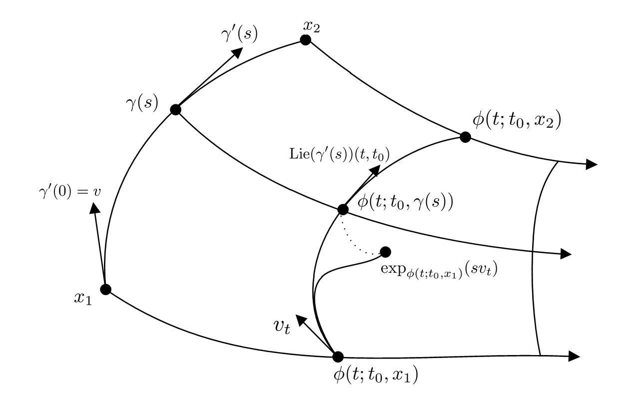
Figure 1: Illustration of the proof

See Fig. 1. for an illustration. Now we want to show that the first term on the right hand side is of order $O(\hat{s}^{2})$. Since $x_{2}=\gamma(\hat{s})$, the term can also be written as

$$\kappa(s)=\frac{d\left(\exp_{\phi(t;t_{0},x_{1})}\left(sv_{t}\right),\phi(t;t_{0},\gamma(s))\right)}{s}$$

where we have replaced $\hat{s}$ with $s$. For this, we consider the two functions $\alpha_{1}(s)=\exp_{\phi(t;t_{0},x_{1})}\left(sv_{t}\right)$, $\alpha_{2}(s)=\phi(t;t_{0},\gamma(s))$. We have $\alpha_{1}(0)=\alpha_{2}(0)=x_{1}$ and $\alpha_{1}^{\prime}(0)=\alpha_{2}^{\prime}(0)=v_{t}.$ Thus

$$\kappa(s)=d(\alpha_{1}(s),\alpha_{2}(s))/s=O(s)$$

invoking Lemma 3. Now letting $\hat{s}\rightarrow 0$ in ( 16), we obtain (12), which completes the proof. ∎

The lower bound of Lie$(v)(t;t_{0})$ is also needed.

Lemma 5.

Suppose that $f$ in (1) is Lipschitz continuous with constant $L$ in the sense of Definition 4, the Lie transport verifies $\left|\text{Lie}(v)(t;t_{0})\right|\geq|v|e^{-L(t-t_{0})},\ \forall v\in T\mathcal{X}.$

Proof.

Let $\gamma(s)=\exp_{x}(sv)$, so $\gamma^{\prime}(0)=v$. From Lemma 2, we have the following inequality for $s>0$:

$$\frac{d(x,\gamma(s))e^{-L(\tau-t)}}{s}\leq\frac{d(\phi(t;t_{0},x)),\phi(t;t_{0},\gamma(s)))}{s},$$

in which the left hand side is nothing but $|v|e^{-L(t-t_{0})}$. Letting $s\rightarrow 0+$,

$$\lim_{s\rightarrow 0+} \frac{d(\phi(t;t_{0},x)),\phi(t;t_{0},\gamma(s)))}{s}$$

$$=\left.\frac{\text{d}}{\text{d}s}\right|_{s=0}d(\phi(t;t_{0},x)),\phi(t;t_{0},\gamma(s)))$$

$$=\lim_{s\rightarrow 0}\left\langle\frac{\partial\phi(t;t_{0},\gamma(s))}{\partial s},\bar{\gamma}^{\prime}(\hat{s})\right\rangle$$

$$\leq\lim_{s\rightarrow 0}\left|\frac{\partial\phi(t;t_{0},\gamma(s))}{\partial s}\right|$$

$$=\left|\text{Lie}(v)(t;t_{0})\right|$$

where $\bar{\gamma}:[0,\hat{s}]\rightarrow\mathcal{X}$ is the normalized geodesic joining $\phi(t;t_{0},x)$ to $\phi(t;t_{0},\gamma(s))$. Thus the proof is completed. ∎

Now we are in position to prove Theorem 3.

Proof of Theorem 3.

Necessity is already proven in Section 3. It remains to prove the converse.

Step 1: We consider the following candidate FLF:

$$V(t,v)=\int_{t}^{t+\delta}\left|\text{Lie}(v)(\tau;t)\right|^{p}\text{d}\tau$$ (17)

where $p\geq 1$, $\delta>0$. From Lemma 2 and Lemma 4, we can estimate the lower and upper bound of $V(t,v)$:

$$V(t,v) \geq|v|^{p}\int_{t}^{t+\delta}e^{-pL(\tau-t)}\text{d}\tau=\frac{1-e^{-pL\delta}}{pL}|v|^{p}$$

$$V(t,v) \leq|v|^{p}\int_{t}^{t+\delta}e^{-p\lambda(\tau-t)}\text{d}\tau=\frac{1-e^{-p\lambda\delta}}{p\lambda}|v|^{p}.$$

Thus there exists two positive constants $c_{1},c_{2}$ such that

$$c_{1}|v|^{p}\leq V(t,v)\leq c_{2}|v|^{p}.$$

Step 2: By the property of Lie transport, we know that

$$\operatorname*{Lie}(\operatorname*{Lie}(v)(t;s))(\tau;t)=\operatorname*{Lie}(v)(\tau;s),$$

so

$$V(s,\text{Lie}(v)(s,t)) =\int_{s}^{s+\gamma}\left|\text{Lie}(\text{Lie }(v)(s,t))(\tau;s)\right|^{p}\text{d}\tau$$

$$=\int_{s}^{s+\delta}\left|\text{Lie}(v)(\tau;t)\right|^{p}\text{d }\tau$$

The timed Lie derivative satisfies

$$\mathcal{L}_{\tilde{f}}V(t,v) =\left.\frac{d}{ds}\right|_{s=t}V(s,\text{Lie}(v)(s,t))$$

$$=\left|\text{Lie}(v)(t+\delta;t)\right|^{p}-\left|v\right|^{p}$$

$$\leq-(1-K^{p}e^{-p\lambda\delta})|v|^{p}$$

$$\leq-\frac{1-K^{p}e^{-p\lambda\delta}}{c_{2}}V(t,v).$$

By choosing $\delta$ large enough such that $1-K^{p}e^{-p\lambda\delta}>0,$ we obtain (8) with $k=(1-K^{p}e^{-p\lambda\delta})/c_{2}$. ∎

Remark 4.

As Theorem 2, the above proof can be extended to Finsler manifold, by replacing the Riemannian metric $g_{ij}$ by $\partial^{2}\left(F^{2}\right)/\partial x_{i}\partial x_{j}$.

Remark 5.

In [30], the authors obtained similar results of Theorem 3 in Euclidean space, see Proposition 1, 2, 3 [30]. More precisely, they proved the equivalence of TULES-NL, UES-TL and ULMTE defined in [30]. We clarify their differences to our results. First, in [30], the state space is $\mathbb{R}^{n}$ with a metric described by positive definite matrices. Compared to Finsler manifolds, it is easier to deal with and excludes some interesting examples, see for example [17]. In contrast, Finsler structure is the key object in this paper, it is more general and admits more complex structures. More importantly, it helps us single out what are the more essential conditions needed to guarantee contraction properties. For example, in [30], it is required that the second order partial derivatives of $f$ are uniformly bounded. On Finsler manifold, this condition is no longer sufficient; instead, conditions imposed on the covariant derivative is needed. See Definition 4. Second, the Lyapunov function constructed in [30] is quite different from the FLF constructed in (17). Thirdly, the proof of Theorem 3 can be easily extended to prove converse theorems of UGIAS systems.

Theorem 4.

Consider the system (1) defined on Riemannian manifold $(\mathcal{X},g)$ with $f\in\mathcal{C}^{2}$ and global Lipschitz continuous with constant $L$ in the sense of Definition 4. If the system is UGIAS, and that the function $\beta(r,s)$ in (4) can be chosen such that $\lim_{h\to 0+}\frac{\beta(h,t)}{h}=\beta^{\prime}(0,t)$ holds uniformly in $t\geq 0$, then there exists a (possibly time dependent) $\mathcal{C}^{0}$ FLF, $V(t,v):\mathbb{R}_{+}\times T\mathcal{X\rightarrow}\mathbb{R}$ such that:

1. There exist two class $\mathcal{K}_{\infty}$ functions $\gamma_{i}$, $i=1,2,$ such that

   $$\gamma_{1}\left(|y|\right)\leq V(t,v)\leq\gamma_{2}\left(|y|\right),\ \forall v\in T\mathcal{X}$$

   where $|\cdot|$ is the norm induced by the Riemannian metric.

2. The timed Lie derivative of $V(t,v)$ along the system (6 ) satisfies

   $$\mathcal{L}_{\tilde{f}}V(t,v)\leq-\gamma_{3}(V(t,v))$$

   for some class $\mathcal{K}_{\infty}$ functions $\gamma_{3}$.

Proof.

To streamline the proof, we prove the theorem in Euclidean space. Thanks to Lemma 1, in Euclidean space, the complete lifted system is

$$\dot{x}=f(x,t),\;\dot{y}=\frac{\partial f(x,t)}{\partial x}y.$$ (18)

Denote the solution with initial time $t$ and initial state $(x,y)$ as $(\phi_{X}^{T}(\tau;t,x),\phi_{Y}^{T}(\tau;t,x,y))^{T}$. It is well known that $\frac{\partial\phi_{X}}{\partial x}(\tau;t,x)$ satisfies the matrix ODE,

$$\dot{X}=\frac{\partial f(\tau,\phi_{X}(\tau;t,x))}{\partial x}X,\ X(t)=I$$

i.e. $\frac{\partial\phi_{X}(\tau;t,x)}{\partial x}=\Phi(\tau,t)$, where $\Phi(\tau,t)$ is the transition matrix corresponding to $\frac{dz}{d\tau}=\frac{\partial f(\tau,\phi_{X}(\tau;t,x))}{\partial x}z$ and hence

$$\phi_{Y}(\tau;t,x,y)=\frac{\partial\phi_{X}(\tau;t,x)}{\partial x}y.$$

By assumption,

$$|\phi_{X}(\tau;t,x_{1})-\phi_{X}(\tau;t,x_{2})|\leq\beta(|x_{1}-x_{2}|,\tau-t),$$ (19)

for all $x_{1},x_{2}\in\mathbb{R}^{n}$ and $\tau\geq t$ and a class $\mathcal{KL}$ function $\beta$. We have the following estimations:

$$\left|\frac{\partial\phi_{X}(\tau;t,x)}{\partial x_{i}}\right| =\left|\lim_{h\rightarrow 0+}\frac{\phi_{X}(\tau;t,x+he_{i})-\phi_{X}(\tau;t,x)}{h}\right|$$

$$=\lim_{h\rightarrow 0+}\frac{|\phi_{X}(\tau;t,x+he_{i})-\phi_{X}(\tau;t,x)|}{h}$$

$$\leq\lim_{h\rightarrow 0+}\frac{\beta(h,\tau-t)}{h}$$

$$=\beta^{\prime}(0,\tau-t)$$

where $\beta^{\prime}$ is the right-derivative of $\beta$ with respect to the first argument, $e_{i}$ is the $i$-th component of the standard basis of $\mathbb{R}^{n}$ and in the second equality we have used the fact that the Euclidean norm is a continuous function so that $|\lim_{x\rightarrow y}g(x)|=\lim_{x\rightarrow y}|g(x)|$. Hence, there holds

$$\left|\frac{\partial\phi_{X}(\tau;t,x)}{\partial x}\right|\leq c\beta^{\prime}(0,\tau-t)$$

for all $x\in\mathbb{R}^{n}$ and $\tau\geq t$, where $c$ is a positive constant. Consequently

$$|\phi_{Y}(\tau;t,x,y)|=\left|\frac{\partial\phi_{X}(\tau;t,x)}{\partial x}y\right|\leq c\beta^{\prime}(0,\tau-t)|y|,\ \forall x,y\in\mathbb{R}^{n}.$$

Let $\tilde{\beta}(r,s):=c\beta^{\prime}(0,s)r$, then $\tilde{\beta}$ is a class $\mathcal{KL}$ function since 1) $r\mapsto c\beta^{\prime}(0,s)r$ is class $\mathcal{K}$ and 2) $s\mapsto c\beta^{\prime}(0,s)r$ is decreasing for $\beta^{\prime}$ is the derivative with respect to the first argument and $\beta(r,\cdot)$ is decreasing for fixed $r$, since by assumption

$$\lim_{s\rightarrow\infty}\beta^{\prime}(0,s)=\lim_{s\rightarrow\infty}\lim_{h\rightarrow 0+}\frac{\beta(h,s)}{h}=\lim_{h\rightarrow 0+}\lim_{s\rightarrow\infty}\frac{\beta(h,s)}{h}=0.$$

Now Proposition 7 [31] implies the existence of two class $\mathcal{K}_{\infty}$ functions $\alpha_{1},\alpha_{2}$ such that

$$\alpha_{1}\left(\tilde{\beta}(r,s)\right)\leq\alpha_{2}(r)e^{-s}.$$

Define the candidate FLF as

$$V(t,x,y)=\int_{t}^{\infty}\alpha_{1}\left(|\phi_{Y}(\tau;t,x,y)|\right)\text{d}\tau,$$

which has the $\alpha_{2}(|y|)$ as upper bound:

$$V(t,x,y)\leq\int_{t}^{\infty}\alpha_{2}(|y|)e^{-(\tau-t)}\text{d}\tau=\alpha_{2}(|y|),$$

so $V$ is well-defined. It also has the lower bound (see Step 1 in the proof of Theorem 2) :

$$V(t,x,y) \geq\int_{t}^{\infty}\alpha_{1}\left(|y|e^{-L(\tau-t)}\right)\text{d}\tau$$

$$=\int_{0}^{\infty}\alpha_{1}\left(|y|e^{-Ls}\right)\text{d}s$$

$$:=\alpha_{3}(\left|y\right|),$$

where $\alpha_{3}$ is class $\mathcal{K}_{\infty}$ since $\alpha_{1}$ is class $\mathcal{K}_{\infty}$. More precisely,

$$\int_{0}^{\infty}\alpha_{1}(|y|e^{-Ls})ds \geq\int_{0}^{1}\alpha_{1}(|y|e^{-Ls})ds$$

$$\geq\int_{0}^{1}\alpha_{1}(|y|e^{-L})ds$$

$$=\alpha_{1}(|y|e^{-L})\rightarrow\infty$$

as $|y|\rightarrow\infty$. Additionally, $\alpha_{3}$ being class $\mathcal{K}$ is obvious. Similar to Step 2 above, we can calculate the Lie derivative of $V(t,x,y)$ along the complete lift system (18) as follows.

$$\mathcal{L}_{\tilde{f}} V(t,x,y)=\left.\frac{\partial}{\partial\tau}\right|_{\tau=t}V(\tau;\phi_{X}(\tau;t,x),\phi_{Y}(\tau;t,x,y))$$

$$=\left.\frac{\partial}{\partial\tau}\right|_{\tau=t}\int_{\tau}^{\infty}\alpha_{1}(|\phi_{Y}(s;\tau,\phi_{X}(\tau;t,x),\phi_{Y}(\tau;t,x,y))|)ds$$

$$=\left.\frac{\partial}{\partial\tau}\right|_{\tau=t}\int_{\tau}^{\infty}\alpha_{1}(|\phi_{Y}(s;t,x,y)|)ds$$

$$=-\alpha_{1}(|y|)$$

Summarizing,

$$\mathcal{L}_{\tilde{f}}V=-\alpha_{1}(|y|)\leq\alpha_{1}(\alpha_{3}^{-1}(V)),$$

hence $V$ is indeed a FLF. Now letting $\gamma_{1}=\alpha_{3},\gamma_{2}=\alpha_{2}$ and $\gamma_{3}=\alpha_{1}\circ\alpha_{3}^{-1}$ will finish the proof. ∎

Remark 6.

The technical assumption of the differentiability of $\beta$ at $(0,s)$ is not very restrictive. It excludes only the case when the graph of $\beta(r,*)$ is tangent to the vertical axis at the origin. However, uniformly differentiability of $\beta(\cdot,s)$ at the origin is an indeed strong assumption which makes this theorem less interesting compared to the integral form proved in [4, Theorem 1]. We do not know whether a smooth $\mathcal{KL}$ function can be constructed when the system is UGIAS, even when the system is smooth.

5 Rediscovery and Extension of Krasovskii’s method

When a UGIES system has $x_{\ast}$ as an equilibrium point, i.e. $f(x_{\ast},t)=0$. It is obvious that the system is exponentially stable. The converse Lyapunov theorem (see e.g. [32]) tells us that there should exist a Lyapunov function $W(t,x)$ (not a FLF) for the system (1) along which, the time derivative of the Lyapunov function is negative definite. Now, having the UGIES property at hand, by Theorem 3, a FLF can be constructed. A natural question is, can we construct a Lyapunov function based on the information of this FLF? The following proposition gives a rather interesting answer. As we will see, it is a rediscovery and extension of the classical Krasovskii’s method used for the construction of Lyapunov function [32].

Theorem 5.

Suppose the system $\dot{x}=f(x,t)$ is UGIES with a FLF $V(t,v)$ with respect to the system (1) and have an equilibrium point $x_{\ast}$. Then the system is UGES. Given a smooth time invariant vector field $h$ on $\mathcal{X}$. If $[f,h]=0$, and

$$k_{1}d(x,x_{\ast})^{q}\leq\left|h(x)\right|\leq k_{2}d(x,x_{\ast})^{q}$$

for $q\geq 1$, then the function $W(t,x)=V(t,h)$ (or $V(t,x,h(x))$) is a Lyapunov function for the system.

We need the following lemma to prove the theorem, which is interesting in its own right.

Lemma 6.

Consider the system $\dot{x}=f(x,t)$ to which the solution is denoted as $\phi(t;t_{0},x_{0})$. If there exists a vector field $h(x)$ on $\mathcal{X}$ such that $[f,h]=0$, then $h(\phi(t;t_{0},x_{0}))\in T_{\phi(t;t_{0},x_{0})}\mathcal{X},\ \forall t\geq t_{0}$ is the unique solution to the system (6) with initial condition $(t_{0};x_{0},h(x_{0}))$. In particular, the solution to (1) started from $(x_{0},f(t_{0},x_{0}))$ is col$(\phi(t;t_{0},x_{0}),f(\phi(t;t_{0},x_{0}),t_{0}))$.

Proof.

The Lie bracket of $f$ and $h$ can be calculated as

$$[f,h](\phi(t;t_{0},x_{0}))=\left.\frac{\text{d}(\phi^{\ast}h)}{\text{ d}s}\right|_{s=t}(\phi(t;t_{0},x_{0}))=0.$$

Thus $\phi^{\ast}h(\phi(t;t_{0},x_{0}))=\text{constant}=(x_{0},h(x_{0})),$ or

$$h(\phi(t;t_{0},x_{0}))=\phi(t;t_{0},x_{0})_{\ast}(x_{0},h(x_{0}))=\text{Lie}(h(x_{0}))(t,t_{0}).$$

which completes the first half of the lemma. Since $[f,f]=0$ is always true, the last claim also follows. ∎

Proof of Theorem 5.

It can be readily checked that $W(t,x)$ is a positive definite Lyapunov candidate. Using the above lemma, we have

$$\mathcal{L}_{f}W(t,x) =\left.\frac{\text{d}}{\text{d}\tau}\right|_{\tau=t}V(\tau,h(\phi(\tau;t,x)))$$

$$=\mathcal{L}_{\tilde{f}}V(t,h(x))$$

$$\leq-kV(t,h(x))$$

$$=-kW(t,x),$$

showing that $W(t,x)$ is indeed a Lyapunov function. ∎

Corollary 1.

Consider the system $\dot{x}=f(x,t)$, where $x\in\mathbb{R}^{n}$, with $f(0,t)=0$. If the system is ULIES with a FLF $V(t,x,\delta x)$. Assume that there exists a smooth vector field $h(x)$ on $\mathbb{R}^{n}$ such that $[f,h]=0$, where $h=0$ if and only if $x=0$, then the function $W(t,x)=V(t,x,h(x))$ is a Lyapunov function such that the system is exponentially stable. In particular, $W(t,x)$ can be chosen as $V(t,x,f(x))$ when the system is time invariant.

Proof.

The time derivative of $W(t,x)$ reads

$$\dot{W}(t ,x)=\dot{V}(t,x,h(x))$$

$$=\frac{\partial V(t,x,h(x))}{\partial t}+\frac{\partial V(t,x,h(x))}{\partial x}f(x,t)$$

$$\;\;+\frac{\partial V(t,x,h(x))}{\partial\delta x}\frac{\partial h(x)}{\partial x}f(x,t)$$

$$=\frac{\partial V(t,x,h(x))}{\partial t}+\frac{\partial V(t,x,h(x))}{\partial x}f(x,t)$$

$$\;\;+\frac{\partial V(t,x,h(x))}{\partial\delta x}\frac{\partial f(x,t)}{\partial x}h(x)$$

$$\leq-kV(t,x,h(x))$$

$$=-kW(t,x),$$

where the third equality follows from the fact in Euclidean space,

$$[f,h]=\frac{\partial f}{\partial x}h-\frac{\partial h}{\partial x}f.$$

Thus we see the system is exponentially stable with Lyapunov function $W(t,x)$. ∎

Theorem 5 recovers and extends the so called Krasovskii’s method [32]: if there exists two constant positive definite matrices $P$ and $Q$ such that

$$P\frac{\partial f(x)}{\partial x}+\left[\frac{\partial f(x)}{\partial x}\right]^{T}P\leq-Q,$$ (20)

then $V(x)=f^{T}(x)Pf(x)$ can serve as a Lyapunov function for the system since $h$ can be taken as $f$. Clearly, if (20) is satisfied, $\delta^{T}xP\delta x$ is a FLF for the system. Then the Krasovskii’s method is a direct consequence of Corallary 1. We consider two examples.

Example 1.

Consider the linear system $\dot{x}=Ax$. Suppose there exists a FLF $V=\delta x^{T}P\delta x$, such that $A^{T}P+PA=-I.$ Then since $[Ax,x]=0$, Corallary 1 tells us that when replacing $\delta x$ with $x$, $V$ becomes a Lyapunov function, i.e. $W(x)=x^{T}Px$. Furthermore, $x^{T}B^{T}PBx$ is also a Lyapunov function as long as $B$ commutes with $A$ since in this case $[Ax,Bx]=(BA-AB)x=0$.

Example 2.

We consider the case when the matrix measure of the Jacobian $J(t,x)=\partial f(x,t)/\partial x$ is uniformly bounded. That is

$$\mu(J(t,x))\leq-c<0,\ \forall t\geq 0,\forall x$$

This is considered in for example [16]. The FLF can be chosen as $V(x,\delta x)=|\delta x|$, and the Lyapunov function $W(t,x)=|f(x,t)|$. Indeed, it can be readilty checked that

$$\dot{W}(t ,x(t))=\lim_{h\rightarrow 0+}\frac{|f(t,x+hf(x))|-|f(x,t)|}{h}$$

$$=\lim_{h\rightarrow 0+}\frac{1}{h}\left(\left|f(x,t)+h\frac{\partial f(t,\xi)}{\partial x}f(x,t)\right|-|f(x,t)|\right)$$

$$\leq\lim_{h\rightarrow 0+}\frac{\left|I+hJ(t,\xi)\right|-1}{h}|f(x,t)|$$

$$=\mu(J(t,\xi))|f(x,t)|$$

$$\leq-cW(t,x(t)).$$

We see that although $f$ is time dependent, $V(t,x,f(x,t))$ may also have the possibility to be a Lyapunov funtion. This sugggests that other tools are needed to analyze such situation.

Remark 7.

We remark that the results obtained by F. Bullo [26] and K. Kosaraju [33] (when the input $u$ is $0$) regarding Krasovskii’s method are special cases of Corallary 1 .

6 Conclusion

Based on the paper [17], we have given further geometric and Lyapunov characterizations of incremental stability by studying the complete lift of the system. We have shown that contraction analysis can be carried out in a coordinate free way. Two converse contraction theorems on Finsler manifolds, namely, UIES (UIAS) implies the existence of a FLF. This result also confirms the differential framework proposed by F. Forni et al. is appropriate for analyzing incremental stability. The third contribution is the establishment of the connections between incremental stability and stability (of an equilibrium), which rediscovers and extends the classical Krasovskii’s method for constructing Lyapunov functions. Further research includes applications of the proposed theories to observer design on manifolds.

7 Acknowlegement

We thank Dr. Antoine Chaillet, Dr. Romeo Ortega, Dr. Fulvio Forni and Dr. John W. Simpson-Porco for fruitful discussions during the preparation of the manuscript.

References

- [1] D. Wu and G.-R. Duan, “Further geometric and lyapunov characterizations of incrementally stable systems on finsler manifolds,” IEEE Transactions on Automatic Control, 2021.
- [2] J. LaSalle, “A study of synchronous asymptotic stability,” Annals of Mathematics, pp. 571–581, 1957.
- [3] J.-L. Salle, Stability by Liapunov’s direct method with applications. Academic Press, 1961.
- [4] D. Angeli, “A lyapunov approach to incremental stability properties,” IEEE Transactions on Automatic Control, vol. 47, no. 3, pp. 410–421, 2002.
- [5] B. S. Rüffer, N. Van De Wouw, and M. Mueller, “Convergent systems vs. incremental stability,” Systems & Control Letters, vol. 62, no. 3, pp. 277–285, 2013.
- [6] B. P. Demidovich, “Dissipativity of a system of nonlinear differential equations in the large,” Uspekhi Matematicheskikh Nauk, vol. 16, no. 3, pp. 216–216, 1961.
- [7] ——, “Lectures on stability theory,” 1967.
- [8] W. Lohmiller and J.-J. E. Slotine, “On contraction analysis for non-linear systems,” Automatica, vol. 34, no. 6, pp. 683–696, 1998.
- [9] J.-J. E. Slotine and W. Wang, “A study of synchronization and group cooperation using partial contraction theory,” in Cooperative Control. Springer, 2005, pp. 207–228.
- [10] W. Wang and J.-J. E. Slotine, “On partial contraction analysis for coupled nonlinear oscillators,” Biological Cybernetics, vol. 92, no. 1, pp. 38–53, 2005.
- [11] A. Pavlov and L. Marconi, “Incremental passivity and output regulation,” Systems & Control Letters, vol. 57, no. 5, pp. 400–409, 2008.
- [12] R. Reyes-Báez, A. van der Schaft, and B. Jayawardhana, “Virtual differential passivity based control for tracking of flexible-joints robots,” IFAC-PapersOnLine, vol. 51, no. 3, pp. 169–174, 2018.
- [13] W. Lohmiller and J.-J. E. Slotine, “Nonlinear process control using contraction theory,” AIChE journal, vol. 46, no. 3, pp. 588–596, 2000.
- [14] J. Jouffroy and T. I. Fossen, “A tutorial on incremental stability analysis using contraction theory,” Modeling, Identification and Control, vol. 31, no. 3, p. 93, 2010.
- [15] E. D. Sontag, “Contractive systems with inputs,” in Perspectives in mathematical system theory, control, and signal processing. Springer, 2010, pp. 217–228.
- [16] Z. Aminzare and E. D. Sontag, “Contraction methods for nonlinear systems: A brief introduction and some open problems,” in 53rd IEEE Conference on Decision and Control. IEEE, 2014, pp. 3835–3847.
- [17] F. Forni and R. Sepulchre, “A differential lyapunov framework for contraction analysis,” IEEE Transactions on Automatic Control, vol. 59, no. 3, pp. 614–628, 2014.
- [18] D. Wu and G.-r. Duan, “Intrinsic construction of lyapunov functions on riemannian manifold,” arXiv preprint arXiv:2002.11384, 2020.
- [19] M. P. d. Carmo, Riemannian Geometry. Birkhäuser, 1992.
- [20] R. Abraham, J. E. Marsden, and T. Ratiu, Manifolds, tensor analysis, and applications. Springer Science & Business Media, 2012, vol. 75.
- [21] K. Yano and S. Ishihara, Tangent and cotangent bundles: differential geometry. Dekker, 1973, vol. 16.
- [22] M. Crampin and F. Pirani, Applicable Differential Geometry. Cambridge University Press, 1986, vol. 59.
- [23] J. Cortés, A. Van Der Schaft, and P. E. Crouch, “Characterization of gradient control systems,” SIAM Journal on Control and Optimization, vol. 44, no. 4, pp. 1192–1214, 2005.
- [24] A. van der Schaft, “A geometric approach to differential hamiltonian systems and differential riccati equations,” in 2015 54th IEEE Conference on Decision and Control (CDC). IEEE, 2015, pp. 7151–7156.
- [25] ——, “On differential passivity.” in NOLCOS, 2013, pp. 21–25.
- [26] F. Bullo and A. D. Lewis, Geometric Control of Mechanical Systems: Modeling, Analysis, and Design for Simple Mechanical Control Systems. Springer, 2019, vol. 49.
- [27] J. W. Simpson-Porco and F. Bullo, “Contraction theory on riemannian manifolds,” Systems & Control Letters, vol. 65, pp. 74–80, 2014.
- [28] Y. Kawano, B. Besselink, and M. Cao, “Contraction analysis of monotone systems via separable functions,” IEEE Transactions on Automatic Control, 2019.
- [29] D. Wu and G. Duan, “On geometric and lyapunov characterizations of incremental stable systems on finsler manifolds,” arXiv preprint arXiv:2002.11444, 2020.
- [30] V. Andrieu, B. Jayawardhana, and L. Praly, “Transverse exponential stability and applications,” IEEE Transactions on Automatic Control, vol. 61, no. 11, pp. 3396–3411, 2016.
- [31] E. D. Sontag, “Comments on integral variants of iss,” Systems & Control Letters, vol. 34, no. 1-2, pp. 93–100, 1998.
- [32] H. K. Khalil, Nonlinear Systems. Upper Saddle River, 2002.
- [33] K. C. Kosaraju, Y. Kawano, and J. Scherpen, “Differential passivity based dynamic controllers,” arXiv preprint arXiv:1907.07420, 2019.