Gödel spacetime, planar geodesics and the Möbius map

Abstract

Timelike geodesics on a hyperplane orthogonal to the symmetry axis of the Gödel spacetime appear to be elliptic-like if standard coordinates naturally adapted to the cylindrical symmetry are used. The orbit can then be suitably described through an eccentricity-semi-latus rectum parametrization, familiar from the Newtonian dynamics of a two-body system. However, changing coordinates such planar geodesics all become explicitly circular, as exhibited by Kundt’s form of the Gödel metric. We derive here a one-to-one correspondence between the constants of the motion along these geodesics as well as between the parameter spaces of elliptic-like versus circular geodesics. We also show how to connect the two equivalent descriptions of particle motion by introducing a pair of complex coordinates in the 2-planes orthogonal to the symmetry axis, which brings the metric into a form which is invariant under Möbius transformations preserving the symmetries of the orbit, i.e., taking circles to circles.

1 Introduction

The geometrical properties and physical aspects of Gödel spacetime Godel:1949ga which make it the prototype for rotating cosmological models have been investigated in depth in the literature since its discovery, leading to the introduction of several coordinate systems which are better suited for showing its various properties (see, e.g., Refs. kundt ; chandra ; Novello:1992hp ; Obukhov:2000jf ; Grave:2009zz ; Bini:2014uua ). Cylindrical-like coordinates are naturally adapted to the cylindrical symmetry of the spacetime about one particular dust particle world line Hawell . The dust source particles are at rest with respect to these coordinates, but form a family of twisting world lines, so that the cylindrical symmetry of the spacetime is preserved about every point. Timelike geodesics on a “planar” 2-surface orthogonal to the symmetry axis appear to be closed elliptic-like curves, which are of different types depending on the value of the ratio between the particle’s conserved angular momentum ($L$) and energy $(E)$ Novello:1982nc . We have recently introduced an eccentricity-semi-latus rectum ($e,p$) parametrization to describe the motion in close analogy with the Newtonian dynamics of a two-body system Bini:2019xpv . For each class of orbits we have then computed gauge-invariant quantities, like the periastron advance and the precession angle of a test gyroscope, thus providing coordinate-independent information. The shape of the orbit, however, is instead coordinate-dependent. The Kundt form of the Gödel metric kundt makes the orbits of all such planar geodesics explicitly circular.

The goal of this article is to derive a one-to-one correspondence between the constants of the motion and parameter spaces of the planar geodesics in the two different forms of the Gödel metric mentioned above, i.e., the standard cylindrical form and Kundt’s form. We will also show how to connect the two equivalent descriptions of particle motion by introducing a pair of complex coordinates in the 2-planes orthogonal to the symmetry axis, which brings the metric into a form which is invariant under Möbius transformations preserving the shape of the orbit, i.e., taking circles to circles.

2 Planar timelike geodesics in the Gödel spacetime

The Gödel spacetime Godel:1949ga ; Hawell is a Petrov type D stationary axisymmetric solution of the nonvacuum Einstein equations with a negative cosmological constant and matter in the form of dust, whose gravitational attraction is balanced by a global rotation. The stress-energy tensor is then $T=\rho\,u\otimes u$, with constant energy density $\rho$ and unit 4-velocity $u$ of the fluid particles aligned with the time coordinate lines, whereas the cosmological constant has the value $\Lambda=-\omega^{2}=-4\pi\rho$. Gödel spacetime is spacetime-homogeneous with five Killing vector fields which allow an infinite number of spatially homogeneous slicing families, each valid within a given neighborhood of some central world line. Changing “spatial” coordinate systems inevitably changes the time slicing family as well.

2.1 Cylindrical-like standard form and elliptic-like curves

Using standard coordinates $(t,r,\phi,z)$ naturally adapted to the cylindrical symmetry Hawell , the Gödel metric reads

$$ds^{2} = \frac{2}{\omega^{2}}\left[-dt^{2}+dr^{2}+\sinh^{2}r(1-\sinh^{2}r)\,d\phi^{2}\right.$$ (1)

$$\qquad\left.+2\sqrt{2}\sinh^{2}r\,dt\,d\phi+dz^{2}\right]$$

$$= \frac{2}{\omega^{2}}\left[-(dt-\sqrt{2}\sinh^{2}r\,d\phi)^{2}+dz^{2}\right.$$

$$\qquad\left.+dr^{2}+\sinh^{2}r(1+\sinh^{2}r)\,d\phi^{2}\right]\,,$$

where the latter form is the orthogonal decomposition adapted to the time coordinate lines imbedded in the dust. The coordinates here are all dimensionless, while the scaling factor $\omega>0$ has the dimension of inverse length and describes the vorticity of the dust world lines which rotate in the increasing $\phi$ direction about the central world line of the coordinate grid.

The horizon radius

$$r_{h}=\ln(1+\sqrt{2})\approx 0.88137\,,\qquad\sinh r_{h}=1\,,\quad\cosh r_{h}=\sqrt{2}\,,$$ (2)

is defined by the condition $g_{\phi\phi}=0$, where the $\phi$ coordinate circles are null and beyond which they are timelike. This radius delimits the “physical region” of the spacetime for the given system of coordinates, if one wants to avoid closed timelike curves.

The Killing vectors associated with the spacetime symmetries are

$$\xi_{1} = \partial_{t}\,,\quad\xi_{2}=\partial_{\phi}\,,\quad\xi_{3}=\partial_{z}\,,$$

$$\xi_{4} = \sqrt{2}\tanh(r)\cos\phi\,\partial_{t}-\sin\phi\,\partial_{r}-\frac{2\cos\phi}{\tanh(2r)}\,\partial_{\phi}\,,$$

$$\xi_{5} = \sqrt{2}\tanh(r)\sin\phi\,\partial_{t}+\cos\phi\,\partial_{r}-\frac{2\sin\phi}{\tanh(2r)}\,\partial_{\phi}\,.$$ (3)

Introduce the 4-vector

$$\eta=\sqrt{2}\tanh(r)\partial_{t}-\frac{2}{\tanh(2r)}\,\partial_{\phi}\,,\qquad||\eta||^{2}=\frac{1}{\omega^{2}}(3-\cosh(4r))\,,$$ (4)

which is spacelike in the region $0<r<r_{*}=\frac{1}{4}{\rm arccosh}(3)\approx 0.44069$ and timelike for $r_{*}<r<r_{h}$. The Killing vectors $\xi_{4}$ and $\xi_{5}$ thus correspond to a rotation in the plane $r-\phi$

$$\begin{pmatrix}-\xi_{5}\\ -\xi_{4}\end{pmatrix}=\begin{pmatrix}-\cos\phi&-\sin\phi\\ \sin\phi&-\cos\phi\end{pmatrix}\begin{pmatrix}\partial_{r}\\ \eta\end{pmatrix}\,.$$ (5)

Near the origin in the polar plane where $\eta\sim\partial_{\phi}$, this azimuthal rotation of the frame vectors $(\partial_{r},\eta)$ aligns $(-\xi_{5},-\xi_{4})$ with the corresponding Cartesian frame $(\partial_{x},\partial_{y})$ defined in the usual way with respect to $(r,\phi)$, representing two translational Killing vector fields in that plane, though tilted with respect to the time coordinate hypersurfaces. In fact when one spatially “translates” the symmetry axis at the origin of these polar coordinates where the time slicing is orthogonal to the time lines, this tilting of these two Killing vectors leads to a new slicing with the same property at the new location.

The geodesic equations are separable and the covariant 4-velocity of a general geodesic has the following form

$$U^{\flat}=-E\,dt+L\,d\phi+b\,dz+U_{r}\,dr\,,$$ (6)

where

$$U_{r}=\frac{2}{\omega^{2}}U^{r}=\frac{2}{\omega^{2}}\frac{dr}{d\lambda}\,,$$ (7)

with $\lambda$ denoting an affine parameter and normalization condition $U^{\alpha}U_{\alpha}=-\mu^{2}$, with $\mu^{2}=1,0,-1$ for timelike, null, spacelike geodesics, respectively. The geodesic equations expressed in terms of the constants of the motion $E=-U\cdot\partial_{t}$, $L=U\cdot\partial_{\phi}$ and $b=U\cdot\partial_{z}$ are

$$\frac{dt}{d\lambda} = -\frac{1}{2}\omega^{2}\left(E-\frac{\sqrt{2}X}{\cosh^{2}r}\right)\,,$$

$$\left(\frac{dr}{d\lambda}\right)^{2} = -\frac{1}{2}\omega^{2}\mu^{2}-\frac{1}{4}\omega^{4}(b^{2}+E^{2})$$

$$+\frac{1}{4}\omega^{4}\frac{X^{2}}{\cosh^{2}r}-\frac{1}{4}\omega^{4}\frac{L^{2}}{\sinh^{2}r}\,,$$

$$\frac{d\phi}{d\lambda} = -\frac{1}{2}\frac{\omega^{2}}{\sinh^{2}r}\left(\sqrt{2}E-\frac{X}{\cosh^{2}r}\right)\,,$$

$$\frac{dz}{d\lambda} = \frac{1}{2}\omega^{2}b\,,$$ (8)

where $X=\sqrt{2}E+L$. These can be integrated analytically. Additional conserved quantities $k_{4}=U\cdot\xi_{4}$ and $k_{5}=U\cdot\xi_{5}$ associated with the Killing vectors $\xi_{4}$ and $\xi_{5}$ satisfy

$$k_{4}\sin\phi+k_{5}\cos\phi = \frac{1}{\sinh(2r)}[\sqrt{2}E-(X+L)\cosh(2r)]\,,$$

$$k_{4}\cos\phi-k_{5}\sin\phi = U^{r}\,,$$ (9)

which define $r$ as an implicit function of $\phi$. This rotation of the Killing constants aligns the conserved translation Killing momenta with the polar frame momenta.

2.1.1 Newtonian-like parametrization of planar geodesics

Here we only consider the case $b=0$ of “planar” timelike geodesics (choosing $\mu=1$ making $\lambda=\tau$) confined to a constant $z$ hyperplane. The associated 4-velocity is

$$U = \frac{\omega^{2}}{2\cosh^{2}r}\left[\sqrt{2}L+E(2-\cosh^{2}r)\right]\,\partial_{t}+U^{r}\partial_{r}$$ (10)

$$-\frac{\omega^{2}}{2\sinh^{2}r\cosh^{2}r}\left(E\sqrt{2}\sinh^{2}r-L\right)\,\partial_{\phi}\,,$$

where

$$(U^{r})^{2} = \frac{\omega^{2}}{4\sinh^{2}r\cosh^{2}r}\left[-2(\tilde{E}^{2}+1)\cosh^{4}r\right.$$

$$+ \left.2(3\tilde{E}^{2}+2\tilde{E}\tilde{L}+1)\cosh^{2}r-(2\tilde{E}+\tilde{L})^{2}\right]\,,$$

having introduced the following rescaling of $E$ and $L$

$$\tilde{E}=\frac{\omega}{\sqrt{2}}E\geq 1\,,\qquad\tilde{L}=\omega L\,.$$ (12)

The orbits are elliptic-like and can be classified into three different types according to the ratio between angular momentum and energy Novello:1982nc .

In Ref. Bini:2019xpv we have recently introduced an equivalent parametrization of the orbit in terms of a semi-latus rectum $p$ and eccentricity $e$, familiar from Newtonian mechanics (but for the change $r\to\cosh^{2}r$), i.e.,

$$\cosh^{2}r=\frac{p}{1+e\cos\chi}\,,$$ (13)

with $p\geq 1$ and $0\leq e<1$ as usual for elliptical orbits, so that $r=r_{\rm(peri)}$ for $\chi=0$ and $r=r_{\rm(apo)}$ for $\chi=\pi$, i.e.,

$$\cosh^{2}r_{\rm(peri)}=\frac{p}{1+e}\,,\qquad\cosh^{2}r_{\rm(apo)}=\frac{p}{1-e}\,.$$ (14)

The main properties of the different kinds of orbits and the relation between the two parametrizations are summarized below.

1. type I:

   The orbits have $0<r_{\rm(peri)}\leq r\leq r_{\rm(apo)}$ and go around the origin with monotonically decreasing $\phi$ opposing the local rotation of the dust source (no turning point in $\phi$). The orbit becomes circular for $r_{\rm(peri)}=r_{\rm(apo)}$. The angular momentum is always negative $\tilde{L}_{\rm min}\leq\tilde{L}<0$ for fixed values of the energy parameter, with

   $$\tilde{L}_{\rm min}=-\tilde{E}+\frac{1}{\sqrt{2}}\sqrt{\tilde{E}^{2}+1}\,.$$ (15)

   The relation between $(\tilde{E},\tilde{L})$ and $(p,e)$ is

   $$\tilde{E} = \frac{p+{\mathcal{Y}}}{\sqrt{(p-{\mathcal{Y}})^{2}-4p(p-1)}}\,,$$

   $$\tilde{L} = \frac{-2{\mathcal{Y}}}{\sqrt{(p-{\mathcal{Y}})^{2}-4p(p-1)}}\,,$$ (16)

   where ${\mathcal{Y}}=\sqrt{(p-1)^{2}-e^{2}}$.

   The solutions for $t$ and $\phi$ turn out to be

   $$t(\chi) = \frac{1}{\sqrt{2}}\left[\chi-\frac{p+{\mathcal{Y}}}{\sqrt{1-e^{2}}}{\rm arctan}(\psi_{1})\right]\,,$$

   $$\phi(\chi) = -\frac{\chi}{2}-{\rm arctan}(\psi_{2})\,,$$ (17)

   with

   $$\psi_{1}=\sqrt{\frac{1-e}{1+e}}\tan\frac{\chi}{2}\,,\qquad\psi_{2}=\sqrt{\frac{p-1+e}{p-1-e}}\tan\frac{\chi}{2}\,.$$ (18)

2. type II:

   The same as type I, with $r_{\rm(peri)}=0$, and $\cosh^{2}r_{\rm(apo)}=2\tilde{E}^{2}/(\tilde{E}^{2}+1)$, so that the orbits pass through the origin. These orbits have vanishing angular momentum $\tilde{L}=0$ corresponding to $p=1+e$, with $\tilde{E}=\sqrt{{(1+e)}/{(1-3e)}}$.

   The solutions for $t$ and $\phi$ turn out to be

   $$t(\chi) = \frac{1}{\sqrt{2}}\left[\chi-\sqrt{\frac{1+e}{1-e}}{\rm arctan}(\psi_{1})\right]\,,$$

   $$\phi(\chi) = -\frac{\chi}{2}\,.$$ (19)

3. type III:

   In this case the $\phi$-motion has a turning point in the allowed range of $r$, preventing the orbit from making a complete circuit about the origin. The angular momentum is always positive $0<\tilde{L}<L_{h}$ for fixed values of the energy parameter, with

   $$L_{h}=2(\tilde{E}-\sqrt{\tilde{E}^{2}-1})\,.$$ (20)

   The relation between $(\tilde{E},\tilde{L})$ and $(p,e)$ is

   $$\tilde{E} = \frac{p-{\mathcal{Y}}}{\sqrt{(p+{\mathcal{Y}})^{2}-4p(p-1)}}\,,$$

   $$\tilde{L} = \frac{2{\mathcal{Y}}}{\sqrt{(p+{\mathcal{Y}})^{2}-4p(p-1)}}\,.$$ (21)

   The solutions for $t$ and $\phi$ turn out to be

   $$t(\chi) = \frac{1}{\sqrt{2}}\left[\chi+\frac{p-{\mathcal{Y}}}{\sqrt{1-e^{2}}}{\rm arctan}(\psi_{1})\right]\,,$$

   $$\phi(\chi) = -\frac{\chi}{2}+{\rm arctan}(\psi_{2})\,.$$ (22)

In any case the eccentricity is limited to $e<1/3$. Furthermore, the relation between the variable $\chi$ and the proper time $\tau$ is

$$\tan\frac{\chi}{2} = \sqrt{\frac{1+e}{1-e}}\tan\left(\zeta\tau\right)\,,\quad\hbox{or}$$

$$\tau = \frac{1}{\zeta}{\rm arctan}\left(\sqrt{\frac{1-e}{1+e}}\tan\frac{\chi}{2}\right)\,,$$ (23)

with $\chi=0\leftrightarrow\tau=0$ and

$$\zeta=\frac{\omega\sqrt{\tilde{E}^{2}+1}}{\sqrt{2}}\,.$$ (24)

The allowed parameter spaces for both the $(\tilde{L},\tilde{E})$ and $(p,e)$ parametrizations are shown in Fig. 1.

Since the spacetime is homogeneous it is enough to consider geodesics of a given kind, e.g., type II orbits passing through the origin, without any loss of generality. One can then switch to a geodesic of a different kind (type I and III) simply by changing the origin of the cylindrical-like coordinate system. In fact, the classification of the orbits depends on the value of the angular momentum parameter $\tilde{L}$ relative to the origin $r=0$, so that it is always possible to find a new parameter $\tilde{L}^{\prime}$ with respect to the origin $r^{\prime}=0$ of the new coordinate system such that old type II orbits will exhibit the same features as either type I or type III orbits.

The transformation $r\to r-r_{0}=r^{\prime}$ implies that the new orbital parameters $(p^{\prime},e^{\prime})$ are related to the old ones $(p,e)$ by the conditions

$$\cosh^{2}(r^{\prime}{}_{\rm(peri)}+r_{0})=\frac{p}{1+e}\,,\qquad\cosh^{2}(r^{\prime}{}_{\rm(apo)}+r_{0})=\frac{p}{1-e}\,,$$ (25)

and

$$\cosh^{2}r^{\prime}{}_{\rm(peri)}=\frac{p^{\prime}}{1+e^{\prime}}\,,\qquad\cosh^{2}r^{\prime}{}_{\rm(apo)}=\frac{p^{\prime}}{1-e^{\prime}}\,.$$ (26)

In fact, the orbit with old orbital parameters $(p,e)$ is shifted along the radial direction. However, one can recover the usual relation (14) by introducing a new pair of orbital parameters $(p^{\prime},e^{\prime})$ with respect to the new coordinate system. For instance, the new parameters associated with old type II orbits having $p=1+e$ turn out to be

$$p^{\prime} = \cosh^{2}r_{0}\frac{(1+6e+e^{2})\cosh(2r_{0})-4\sqrt{e}(1+e)\sinh(2r_{0})+(1-e)^{2}}{(1+e)^{2}\cosh(2r_{0})-2\sqrt{e}(1+e)\sinh(2r_{0})+(1-e)^{2}}\,,$$

$$e^{\prime} = 2\sqrt{e}\frac{2\sqrt{e}\cosh(2r_{0})-(1+e)\sinh(2r_{0})}{(1+e)^{2}\cosh(2r_{0})-2\sqrt{e}(1+e)\sinh(2r_{0})+(1-e)^{2}}\,,$$ (27)

which reduce to $p^{\prime}=\cosh^{2}r_{0}$ and $e^{\prime}=0$ for $e=0$, corresponding to a circular orbit with radius $r_{0}$, as for type I orbits in the same limiting case of vanishing eccentricity.

$\begin{array}[]{cc}\includegraphics[scale={0.3}]{fig1a.eps}&\qquad\includegraphics[scale={0.3}]{fig1b.eps}\\[5.69046pt] \mbox{(a)}&\qquad\mbox{(b)}\cr\end{array}$

Figure 1: The allowed parameter spaces $(\tilde{L},\tilde{E})$ and $(p,e)$ for planar timelike geodesics in the physical region $r<r_{h}$ are shown in panels (a) and (b), respectively. Type II orbits have $\tilde{L}=0$, corresponding to the line $p=1+e$ where $r_{\rm(peri)}=0$ (see Eq. (14)). The type I ($\tilde{L}_{\rm min}\leq\tilde{L}<0$) and III ($0<\tilde{L}<L_{h}$) orbits are folded over onto each other into the triangular region between the lines $p=1+e$ and $p=2(1-e)$ where $r_{\rm(apo)}=r_{h}$. The upper boundary for type I orbits is implicitly defined by the vanishing of the denominator in Eq. (1), for which these geodesics become null.

2.2 Kundt’s form and circles

The cylindrical standard form (1) of the metric is related to Kundt’s form kundt

$$ds^{2}=-\left(dT+\frac{1}{\omega Y}dX\right)^{2}+\frac{1}{2\omega^{2}Y^{2}}(dX^{2}+dY^{2})+dZ^{2}\,,$$ (28)

by the transformation

$$\omega T = \sqrt{2}t-2\arctan\left(e^{-2r}\tan\frac{\phi}{2}\right)+\phi\,,$$

$$\sqrt{2}\omega(X+iY) = i\frac{1-\tanh re^{-i\phi}}{1+\tanh re^{-i\phi}}\,,\qquad Z=\frac{\sqrt{2}}{\omega}z\,.$$ (29)

We notice the following Killing vectors

$$\Xi_{1}=\partial_{T}\,,\qquad\Xi_{2}=\partial_{X}\,,\qquad\Xi_{3}=X\partial_{X}+Y\partial_{Y}\,,\qquad\Xi_{4}=\partial_{Z}\,,$$ (30)

which are combinations of those associated with the cylindrical-like metric (see Eq. (2.1))

$$\Xi_{1} = \frac{\omega}{\sqrt{2}}\partial_{t}=\frac{\omega}{\sqrt{2}}\xi_{1}\,,$$

$$\Xi_{2} = \omega(\partial_{t}-\sqrt{2}\partial_{\phi})+\sqrt{2}\omega\left[\frac{1}{\sqrt{2}}\tanh(r)\cos\phi\,\partial_{t}-\frac{1}{2}\sin\phi\,\partial_{r}-\frac{\cos\phi}{\tanh(2r)}\partial_{\phi}\right]$$

$$= \omega\left(\xi_{1}-\sqrt{2}\xi_{2}+\frac{1}{\sqrt{2}}\xi_{4}\right)\,,$$

$$\Xi_{3} = -\frac{1}{\sqrt{2}}\tanh(r)\sin\phi\,\partial_{t}-\frac{1}{2}\cos\phi\,\partial_{r}+\frac{\sin\phi}{\tanh(2r)}\partial_{\phi}=-\frac{1}{2}\xi_{5}\,,$$

$$\Xi_{4} = \frac{\omega}{\sqrt{2}}\partial_{z}=\frac{\omega}{\sqrt{2}}\xi_{3}\,.$$ (31)

When expressed in this coordinate system the azimuthal Killing vector $\xi_{2}=\partial_{\phi}$ becomes

$$\xi_{2}=\frac{1}{\omega}(1-\sqrt{2}\omega Y)\partial_{T}-\frac{\sqrt{2}}{4\omega}[1+2\omega^{2}(X^{2}-Y^{2})]\partial_{X}-\sqrt{2}\omega XY\partial_{Y}=\Xi_{5}\,.$$ (32)

The timelike geodesic $4$-velocity vector of the metric (28) is re-expressed as

$$U = -\frac{\sqrt{2}}{C}\left(\frac{Y^{\prime}}{2}-Y\right)\partial_{T}+\frac{\sqrt{2}}{C}\omega Y(Y^{\prime}-Y)\,\partial_{X}$$ (33)

$$+\frac{\sqrt{2}}{C}\omega Y(X-X^{\prime})\,\partial_{Y}+\frac{B}{C}\partial_{Z}\,,$$

i.e.,

$$U^{\flat}=-\frac{Y^{\prime}}{\sqrt{2}C}dT-\frac{1}{\sqrt{2}C\omega}dX+\frac{(X-X^{\prime})}{\sqrt{2}C\omega Y}dY+\frac{B}{C}dZ\,,$$ (34)

with normalization condition ($U^{\alpha}U_{\alpha}=-1$) equivalent to

$$(X-X^{\prime})^{2}+(Y-Y^{\prime})^{2}=\frac{1}{2}(Y^{\prime})^{2}-B^{2}-C^{2}\equiv R^{2}\,,$$ (35)

where $X^{\prime}$, $Y^{\prime}$, $C$ and $B$ are constants associated with the above Killing vectors

$$\Xi_{1}\cdot U = -\frac{Y^{\prime}}{\sqrt{2}C}\,,\qquad\Xi_{2}\cdot U=-\frac{1}{\sqrt{2}\omega C}\,,$$

$$\Xi_{3}\cdot U = -\frac{X^{\prime}}{\sqrt{2}\omega C}\,,\qquad\Xi_{4}\cdot U=\frac{B}{C}\,,$$

$$\Xi_{5}\cdot U = \frac{1}{4\omega^{2}C}[1-2\sqrt{2}\omega Y^{\prime}+2\omega^{2}((X^{\prime})^{2}+(Y^{\prime})^{2}-R^{2})]\,.$$ (36)

Eq. (35) suggests the following parametric equations for the orbit

$$X(\tau)=X^{\prime}+R\cos\alpha(\tau)\,,\qquad Y(\tau)=Y^{\prime}+R\sin\alpha(\tau)\,,\qquad Z(\tau)=\frac{B}{C}\,\tau\,,$$ (37)

which imply

$$\frac{d\alpha(\tau)}{d\tau}=\frac{\sqrt{2}}{C}\omega(Y^{\prime}+R\sin\alpha(\tau))\,,\qquad\frac{dT(\tau)}{d\tau}=\frac{\sqrt{2}}{C}\left(\frac{Y^{\prime}}{2}+R\sin\alpha(\tau)\right)\,,$$ (38)

with solution

$$\alpha(\tau)=2\arctan\left(\frac{Y^{\prime}\tan(\Omega\tau)}{\kappa-R\tan(\Omega\tau)}\right)\,,\qquad\omega T(\tau)=\alpha(\tau)-\frac{Y^{\prime}}{\sqrt{2}C}\omega\tau\,,$$ (39)

where

$$\kappa=\sqrt{(Y^{\prime})^{2}-R^{2}}\,,\qquad\Omega=\frac{\omega}{\sqrt{2}C}\kappa\,,$$ (40)

and initial conditions have been chosen so that $T(0)=0=\alpha(0)$.

Let us now consider planar geodesics corresponding to $B=0$. Applying the coordinate transformation (2.2) to the particle’s 4-velocity then yields the following relation between the constants of motion

$$E=\frac{Y^{\prime}}{\omega C}\,,\qquad L=\frac{C}{2}+\frac{1}{C}\left[\left(\frac{Y^{\prime}}{2}-\frac{1}{\sqrt{2}\omega}\right)^{2}+\frac{(X^{\prime})^{2}}{2}-\frac{1}{4\omega^{2}}\right]\,,$$ (41)

which imply

$$\omega X^{\prime} = \pm\left[-\frac{1}{2}-(\tilde{E}^{2}+1)\tilde{C}^{2}+2(\tilde{E}+\tilde{L})\tilde{C}\right]^{1/2}$$

$$\equiv \pm\sqrt{\tilde{E}^{2}+1}\sqrt{(\tilde{C}-\tilde{C}_{1})(\tilde{C}_{2}-\tilde{C})}\,,$$

$$\omega Y^{\prime} = \sqrt{2}\tilde{E}\tilde{C}\,,$$

$$\omega R = \tilde{C}\sqrt{\tilde{E}^{2}-1}\,,$$ (42)

with $\tilde{C}=\omega C>0$ and $\tilde{C}_{1}\leq\tilde{C}\leq\tilde{C}_{2}$. Because $Y^{\prime}$ is always positive, the centers cannot be located along the $X$-axis. In contrast, they may lie on the $Y$-axis if either $\tilde{C}=\tilde{C}_{1}$ (with $\omega Y^{\prime}_{1}=\sqrt{2}\tilde{E}\tilde{C}_{1}$) or $\tilde{C}=\tilde{C}_{2}$ (with $\omega Y^{\prime}_{2}=\sqrt{2}\tilde{E}\tilde{C}_{2}$). Furthermore, the radius of the orbit is such that $R_{1}\leq R\leq R_{2}$.

Let us study the locus of the centers for type II orbits, for fixed values of $\tilde{C}$. Substituting $\tilde{L}=0$ and $\tilde{E}=\sqrt{{(1+e)}/{(1-3e)}}$ in Eq. (2.2) gives

$$\tilde{C}_{1}=\frac{\sqrt{1-3e}}{2(1-e)}(\sqrt{1+e}-\sqrt{2e})\,,\qquad\tilde{C}_{2}=\frac{\sqrt{1-3e}}{2(1-e)}(\sqrt{1+e}+\sqrt{2e})\,.$$ (43)

Their behavior as functions of $e$ is shown in Fig. 2. Therefore

$$Y^{\prime}_{1}=\frac{\sqrt{1+e}}{\sqrt{2}(1-e)}(\sqrt{1+e}-\sqrt{2e})\,,\qquad Y^{\prime}_{2}=\frac{\sqrt{1+e}}{\sqrt{2}(1-e)}(\sqrt{1+e}+\sqrt{2e})\,,$$ (44)

which become $Y^{\prime}_{1}=1/\sqrt{2}=Y^{\prime}_{2}$ and $Y^{\prime}_{1}=\sqrt{2}-1$, $Y^{\prime}_{2}=\sqrt{2}+1$ in the two limiting cases $e\to 0$ and $e\to 1/3$, respectively. The locus of the centers is shown in Fig. 3.

The radius of the orbit is

$$\omega R=2\tilde{C}\sqrt{\frac{e}{1-3e}}\,,$$ (45)

so that its limiting values are

$$\omega R_{1}=\frac{\sqrt{e}}{1-e}(\sqrt{1+e}-\sqrt{2e})\,,\qquad\omega R_{2}=\frac{\sqrt{e}}{1-e}(\sqrt{1+e}+\sqrt{2e})\,.$$ (46)

The orbit intersects the $Y-$axis at $\omega Y=1/\sqrt{2}$ for every value of $\tilde{C}$ and $e$ and at $\omega Y=2\omega Y^{\prime}-1/\sqrt{2}$. Fig. 4 shows the circles corresponding to type II orbits for a fixed value of $\tilde{C}$ and different values of the eccentricity $e$.

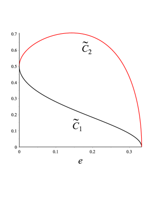
Figure 2: The behavior of the quantities $\tilde{C}_{1}$ and $\tilde{C}_{2}$ as functions of $e$ is shown for orbits of type II.

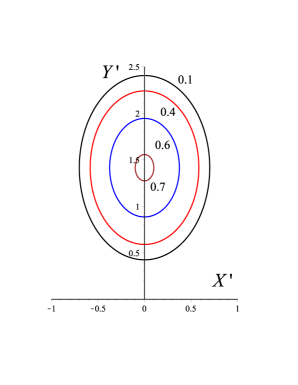
Figure 3: The locus of the centers for type II orbits is shown for selected values of $\tilde{C}=[0.1,0.4,0.6,0.7]$.

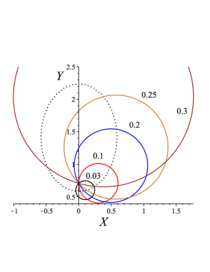
Figure 4: The circles corresponding to type II orbits are shown for $\tilde{C}=0.4$ and selected values of the eccentricity $e=[0.03,0.1,0.2,0.25,0.3]$. The dotted curve is the locus of the centers of Fig. 3. Only positive values of $X^{\prime}$ are taken, for simplicity (see Eq. (2.2)).

3 Möbius transformations

A Möbius transformation $T_{(a,b,c,d)}$ of the complex plane $\mathbb{C}$ has the fractional-linear form

$$T_{(a,b,c,d)}(z)=\frac{az+b}{cz+d}\,,$$ (47)

where $a,b,c,d,z\in{\mathbb{C}}$ are complex numbers and $ad-bc\not=0$. The set of all Möbius transformations is a group under composition. The transformations $S_{(a,b)}(z)=T_{(a,b,0,1)}(z)=az+b$ (setting $d=1$ without loss of generality since one can always take $a\to a/d$, $b\to b/d$) form the subgroup of similarities, whereas the transformation $T_{(0,1,1,0)}(z)=1/z$ is termed an inversion. Every Möbius transformation $T_{(a,b,c,d)}$ can be interpreted as a nonunique combination of a similarity and an inversion.

It is well known that there exists an isomorphism between the Lorentz group SO$(3,1)$ that preserves the orientation of space and the group SL$(2,{\mathbb{C}})$ of conformal transformations of the 2-dimensional sphere, under which Lorentz transformations correspond to conformal transformations of this sphere (see, e.g., Ref. Oblak:2015qia and references therein), represented by complex $2\times 2$ matrices of unit determinant. The basic geometric property of Möbius transformations is that they preserve angles between curves and map circles (and straight lines) into circles (and straight lines).

3.1 Flat spacetime

Consider the Minkowski metric expressed in cylindrical coordinates

$$ds^{2}=-dt^{2}+dr^{2}+r^{2}d\phi^{2}+dz^{2}\,,$$ (48)

simply derived from the standard Cartesian inertial coordinate form

$$ds^{2}=-dt^{2}+dx^{2}+dy^{2}+dz^{2}\,,$$ (49)

using the coordinate transformation $x=r\cos\phi$, $y=r\sin\phi$ in the $x$-$y$ plane. Identifying this real plane with the complex plane with the further transformation $\zeta=x+iy=re^{i\phi}$, the inverse transformation is

$$r=(\zeta\bar{\zeta})^{1/2}\,,\qquad\phi=\frac{1}{2i}\ln\left(\frac{\zeta}{\bar{\zeta}}\right)\,,$$ (50)

which leads to the following expression for the metric (48)

$$ds^{2}=-dt^{2}+d\zeta d\bar{\zeta}+dz^{2}\,,$$ (51)

which remains invariant under the following complex linear transformation

$$\zeta^{\prime}=\sigma\zeta+\beta\,,\qquad\sigma=e^{i\theta}\,,\ \theta\in\mathbb{R}$$ (52)

representing a combined rotation and translation of the $x$-$y$ plane as long as $\sigma$ is a unit complex number. A pure rotation (set $\beta=0$) corresponds to a counterclockwise rotation $\phi\to\phi+\theta$ by the angle $\theta$ in this plane, or

$$(x,y)\to(x\cos\theta-y\sin\theta,x\sin\theta+y\cos\theta)\,.$$ (53)

The Minkowski spacetime timelike geodesics are straight lines representing the world lines of massive test particles of mass $m>0$. If they are parametrized by the proper time $\tau$, assuming that they pass through the point $(x_{0},y_{0},z_{0})$ of the above inertial coordinate system at $\tau=0$, these take the form

$$t=E\tau\,,\qquad x-x_{0}=p_{x}\tau\,,\qquad y-y_{0}=p_{y}\tau\,,\qquad z-z_{0}=p_{z}\tau\,,$$ (54)

with the normalization condition

$$E^{2}=m^{2}+p^{2}\,,\qquad p^{2}=p_{x}^{2}+p_{y}^{2}+p_{z}^{2}$$ (55)

for the associated energy and momentum per unit mass. The momentum 1-form (per unit mass) along the geodesic is

$$P=-Edt+p_{a}dx^{a}\,.$$ (56)

Their representation in cylindrical coordinates centered now at $(x_{0},y_{0},z_{0})$ becomes

$$t=E\tau\,,\qquad r=p_{\perp}\,\tau\,,\qquad\phi=\arctan\left(\frac{p_{y}}{p_{x}}\right)\,,\qquad z-z_{0}=p_{z}\tau\,,$$ (57)

where

$$p_{\perp}=\sqrt{p_{x}^{2}+p_{y}^{2}}\,.$$ (58)

We limit our considerations to orbits on a constant $z$ hyperplane by assuming $p_{z}=0$. The fact that $\phi$ is constant along the motion allows for the parametrization

$$p_{x}=p_{\perp}\cos\phi\,\qquad p_{y}=p_{\perp}\sin\phi\,,\qquad\phi={\rm const}.$$ (59)

or equivalently

$$\zeta=re^{i\phi}=(p_{x}+ip_{y})\,\tau\,,\qquad|\zeta|=p_{\perp}\tau\,.$$ (60)

The effect of the transformation (52) is then

$$\zeta^{\prime}=e^{i\theta}(p_{x}+ip_{y})\,\tau+\beta=(p_{x}^{\prime}+ip_{y}^{\prime})\,\tau+\beta\,,$$ (61)

rotating the momentum directly analogous to Eq. (53)

$$(p_{x}^{\prime},p_{y}^{\prime})=(\cos\theta\,p_{x}-\sin\theta\,p_{y},\sin\theta\,p_{x}+\cos\theta\,p_{y})\,.$$ (62)

Applying the Möebius transformation (47) to the straight lines (54), they are mapped to circles (or again straight lines). In fact, the line (54) for $p_{z}=0$ and $z=z_{0}$, i.e.,

$$p_{y}x-p_{x}y-p_{y}x_{0}+p_{x}y_{0}=0\,,$$ (63)

can be written as

$$\bar{\alpha}\zeta-\alpha\bar{\zeta}-2i(-p_{y}x_{0}+p_{x}y_{0})=0\,,$$ (64)

where

$$\alpha=p_{x}+ip_{y}\,.$$ (65)

The effect of the map $T_{(0,1,1,0)}(\zeta)=1/\zeta$ to Eq. (64) is

$$\frac{\bar{\alpha}}{\zeta}-\frac{\alpha}{\bar{\zeta}}-2i(-p_{y}x_{0}+p_{x}y_{0})=0\,,$$ (66)

i.e.,

$$\bar{\alpha}\bar{\zeta}-\alpha\zeta-2i(-p_{y}x_{0}+p_{x}y_{0})\zeta\bar{\zeta}=0\,,$$ (67)

which is the equation of a circle if $-p_{y}x_{0}+p_{x}y_{0}\not=0$ (or a straight line again if $-p_{y}x_{0}+p_{x}y_{0}=0$)

$$|\zeta-\zeta_{\rm c}|^{2}=\rho^{2}\,,$$ (68)

where

$$\zeta_{\rm c}=-i\frac{\alpha}{2(-p_{y}x_{0}+p_{x}y_{0})}\,,\qquad\rho=|\zeta_{\rm c}|\,.$$ (69)

These circles, however, are no longer geodesics.

3.2 Möbius form of the Gödel metric: taking circles to circles

Analogous to the Minkowski spacetime introduction of a complex variable $\zeta=re^{i\phi}$ in the “polar plane”, define

$$\zeta=\tanh r\,e^{i\phi}\,,$$ (70)

with inverse map

$$r={\rm arctanh}((\zeta\bar{\zeta})^{1/2})=\ln\left(\frac{1+(\zeta\bar{\zeta})^{1/2}}{1-(\zeta\bar{\zeta})^{1/2}}\right)^{1/2}\,,\qquad\phi=\frac{1}{2i}\ln\left(\frac{\zeta}{\bar{\zeta}}\right)\,.$$ (71)

which transforms the cylindrical-like standard metric (1) into the form

$$ds^{2} = \frac{2}{\omega^{2}}\left\{-\left[dt-\frac{i(\zeta d\bar{\zeta}-\bar{\zeta}d\zeta)}{\sqrt{2}(1-\zeta\bar{\zeta})}\right]^{2}+\frac{d\bar{\zeta}d\zeta}{(1-\zeta\bar{\zeta})^{2}}+dz^{2}\right\}\,.$$ (72)

This derivation needs the differentials

$$d\zeta=e^{i\phi}[(1-\tanh^{2}r)dr+i\tanh r\,d\phi]\,,$$

$$\bar{\zeta}d\zeta=\tanh r(1-\tanh^{2}r)dr+i\bar{\zeta}\zeta d\phi\,,$$ (73)

leading to

$$d\phi=\frac{\bar{\zeta}d\zeta-\zeta d\bar{\zeta}}{2i\bar{\zeta}\zeta}\,,\qquad dr=\frac{\bar{\zeta}d\zeta+\zeta d\bar{\zeta}}{2(\zeta\bar{\zeta})^{1/2}(1-\zeta\bar{\zeta})}\,.$$ (74)

Similarly, the complex map

$$\omega T=\sqrt{2}t-i\ln(\zeta)\,,\qquad X=\frac{1}{\zeta}+\bar{\zeta}\,,\qquad Y=i\left(\frac{1}{\zeta}-\bar{\zeta}\right)\,,\qquad\omega Z=\sqrt{2}z\,,$$ (75)

brings Kundt’s form of the metric (28) into the same Möbius form (72).

Successively, the second change of variables

$$t = t^{\prime}+\frac{i\sqrt{2}}{2}\ln\left(\frac{\bar{\alpha}_{0}-\bar{\zeta}^{\prime}\beta_{0}}{\alpha_{0}-\zeta^{\prime}\bar{\beta}_{0}}\right)\,,\qquad\zeta=\frac{\beta_{0}-\zeta^{\prime}\bar{\alpha}_{0}}{-\alpha_{0}+\zeta^{\prime}\bar{\beta}_{0}}\,,$$

$$\bar{\zeta} = \frac{\bar{\beta}_{0}-\bar{\zeta}^{\prime}\alpha_{0}}{-\bar{\alpha}_{0}+\bar{\zeta}^{\prime}\beta_{0}}\,,\qquad z=z\,,$$ (76)

leaves the metric formally invariant, i.e.,

$$ds^{2} = \frac{2}{\omega^{2}}\left\{-\left[dt^{\prime}-\frac{i(\zeta^{\prime}d\bar{\zeta}^{\prime}-\bar{\zeta}^{\prime}d\zeta^{\prime})}{\sqrt{2}(1-\zeta^{\prime}\bar{\zeta}^{\prime})}\right]^{2}+\frac{d\bar{\zeta}^{\prime}d\zeta^{\prime}}{(1-\zeta^{\prime}\bar{\zeta}^{\prime})^{2}}+dz^{2}\right\}\,,$$ (77)

as already discussed in Ref. Bengtsson . Planar timelike geodesics satisfy the equations

$$\dot{t} = \frac{\omega^{2}{\mathcal{E}}}{2}+\frac{i(\zeta\dot{\bar{\zeta}}-\bar{\zeta}\dot{\zeta})}{\sqrt{2}(1-\zeta\bar{\zeta})}\,,$$

$$\dot{\zeta}\dot{\bar{\zeta}} = \frac{\omega^{2}}{2}\left(\frac{\omega^{2}{\mathcal{E}}^{2}}{2}-1\right)(1-\zeta\bar{\zeta})^{2}\,,$$

$$2\zeta\dot{\bar{\zeta}}^{2} = (1-\zeta\bar{\zeta})(i\sqrt{2}\omega^{2}{\mathcal{E}}\dot{\bar{\zeta}}-\ddot{\bar{\zeta}})\,,$$ (78)

where a dot denotes derivative with respect to the proper time $\tau$ and $\mathcal{E}$ is the conserved energy per unit mass of the particle. Circular geodesics $\zeta=Re^{-i\Omega\tau}$ then exist, with

$$R=\frac{\sqrt{\omega^{2}{\mathcal{E}}^{2}+2}-\sqrt{2}\omega{\mathcal{E}}}{\sqrt{\omega^{2}{\mathcal{E}}^{2}-2}}\,,\qquad\Omega=\omega\sqrt{\omega^{2}{\mathcal{E}}^{2}+2}\,,$$ (79)

and

$$t=\left(\frac{\Omega}{\sqrt{2}}-\frac{1}{2}\omega^{2}{\mathcal{E}}\right)\tau\,.$$ (80)

4 Concluding remarks

Planar timelike geodesics of the Gödel spacetime, i.e., their projection on a hyperplane orthogonal to the symmetry axis, have been extensively studied in the literature by using different coordinate systems. Among them is the frequently used choice of cylindrical-like coordinates naturally adapted to the spacetime symmetries. Particle trajectories viewed in these coordinates appear to be elliptic-like and their features can be conveniently studied through an eccentricity-semi-latus rectum $(p,e)$ parametrization familiar (though slightly generalized) from Newtonian mechanics. Such deformed ellipses are of three different kinds, depending on the chosen range of orbital parameters, and correspond to closed curves which either go around the origin (type I) or pass through it (type II) or are centered away from it (type III). Type I orbits may reduce to circles for vanishing eccentricity. However, since the Gödel spacetime is homogeneous, then it must look the same from every point. Therefore, the shape of geodesics about the origin is topologically equivalent to that about any other point chosen as the origin of a new cylindrical-like coordinate system.

The best way to show this feature is to pass to Kundt’s form of the Gödel metric, for which planar geodesics all become circular. We have established here a one-to-one correspondence between the conserved quantities as well as the parameter space of elliptic-like versus circular geodesics: different kinds of elliptic-like orbits turn out to correspond to circles with different loci of the center as well as different radii depending on the allowed range of orbital parameters $p$ and $e$. We have also shown how to connect the two equivalent descriptions of particle motion by introducing a pair of complex coordinates in the 2-planes orthogonal to the symmetry axis, which brings the metric into a form which is invariant under Möbius transformations preserving the symmetries of the orbit, i.e., taking circles to circles.

References

- (1) K. Gödel, “An Example of a new type of cosmological solutions of Einstein’s field equations of gravitation,” Rev. Mod. Phys. 21, 447 (1949). doi:10.1103/RevModPhys.21.447
- (2) W. Kundt, “Trägheitsbahnen in einem von Gödel angegebenen kosmologischen Modell,” Z. Phys. 145, 611 (1956).
- (3) S. Chandrasekhar and J. P. Wright, “The Geodesics in Gödel’s Universe,” Proceedings of the National Academy of Sciences of the United States of America, 47, 341 (1961).
- (4) M. Novello, N. F. Svaiter and M. E. X. Guimaraes, “Synchronized frames for Godel’s universe,” Gen. Rel. Grav. 25, 137 (1993). doi:10.1007/BF00758823
- (5) Y. N. Obukhov, “On physical foundations and observational effects of cosmic rotation,” Published in Colloquium on Cosmic Rotation: Proceedings. Edited by M. Scherfner, T. Chrobok and M. Shefaat (Wissenschaft und Technik Verlag: Berlin, 2000) pp. 23–96 [astro-ph/0008106].
- (6) F. Grave, M. Buser, T. Muller, G. Wunner and W. P. Schleich, “The Gödel universe: Exact geometrical optics and analytical investigations on motion,” Phys. Rev. D 80, 103002 (2009). doi:10.1103/PhysRevD.80.103002
- (7) D. Bini, A. Geralico and R. T. Jantzen, “Separable geodesic action slicing in stationary spacetimes,” Gen. Rel. Grav. 44, 603 (2012). doi:10.1007/s10714-011-1295-2 [arXiv:1408.5259 [gr-qc]]
- (8) S. W. Hawking and G. F. R. Ellis, “The Large Scale Structure of Spacetime,” Cambridge University Press, Cambridge, UK (1973).
- (9) M. Novello, I. D. Soares and J. Tiomno, “Geodesic Motion And Confinement In Gödel’s Universe,” Phys. Rev. D 27, 779 (1983). doi:10.1103/PhysRevD.27.779
- (10) D. Bini, A. Geralico, R. T. Jantzen and W. Plastino, “Gödel spacetime: Planar geodesics and gyroscope precession,” Phys. Rev. D 100, no. 8, 084051 (2019). doi:10.1103/PhysRevD.100.084051 [arXiv:1905.04917 [gr-qc]].
- (11) B. Oblak, “From the Lorentz Group to the Celestial Sphere,” arXiv:1508.00920 [math-ph].
- (12) I. Bengtsson, “Spherical symmetry and black holes,” http://www.fysik.su.se/ ingemar/sfar.pdf.