Initial-State Dependence of Thermodynamic Dissipation for any Quantum Process

Abstract

New exact results about the nonequilibrium thermodynamics of open quantum systems at arbitrary timescales are obtained by considering all possible variations of initial conditions of a system, its environment, and correlations between them. First we obtain a new quantum-information theoretic equality for entropy production, valid for an arbitrary initial joint state of system and environment. For any finite-time process with a fixed initial environment, we then show that the system’s loss of distinction—relative to the minimally dissipative state—exactly quantifies its thermodynamic dissipation. The quantum component of this dissipation is the change in coherence relative to the minimally dissipative state. Implications for quantum state preparation and local control are explored. For nonunitary processes—like the preparation of any particular quantum state—we find that mismatched expectations lead to divergent dissipation as the actual initial state becomes orthogonal to the anticipated one.

I Introduction

Much recent progress extends Landauer’s principle to the quantum regime—affirming that quantum information is physical [1, 2, 3, 4, 5]. Associated bounds refine our understanding of how much heat needs to be exhausted—or how much work needs to be performed, or could be extracted—to preserve the Second Law of Thermodynamics: Entropy production is expected to be non-negative $\bm{\Sigma}_{\rho_{0}}\geq 0$ from any initial density matrix $\rho_{0}$. However, these Landauer-type bounds only become tight in the infinite-time quasistatic limit, as entropy production goes to zero. Yet infinite time is not a luxury afforded to quantum systems with short decoherence time. And, even if coherence can be maintained for significant time-length, we want to know the thermodynamic limits of both quantum computers and natural quantum processes that transform quickly.

Here, we demonstrate a source of heat dissipation beyond Landaur’s bound that applies at any timescale. We illustrate that when engineering any nonunitary process, entropy production always has initial state dependence. It is impossible to optimize resulting entropy production for all input states. Instead, any choice of realization implies some minimally dissipative state $\sigma_{0}$. The injection of any other input state, $\rho_{0}$, results in extra dissipation quantified by

$$\bm{\Sigma}_{\rho_{0}}-\bm{\Sigma}_{\sigma_{0}}=k_{\text{B}}\text{D}\bigl{[}\rho_{0}\big{\|}\sigma_{0}\bigr{]}-k_{\text{B}}\text{D}\bigl{[}\rho_{\tau}\big{\|}\sigma_{\tau}\bigr{]}~{},$$ (1)

the contraction of the relative entropy between the actual input state $\rho_{0}$ and the minimally dissipative input $\sigma_{0}$ over the time-interval $\tau$ in which the process is applied. This dissipation is additional to that given by Landauer, and generalizes a theorem by Kolchinsky and Wolpert for classical computation to scenarios where quantum coherence can play a significant role [6].

We then highlight some immediate consequences. First, our result implies entropy production for almost all inputs to any reset protocol. Second, it implies a thermodynamic cost to misaligned expectations: To minimize heat dissipation, one should tailor the implementation of a desired quantum operation to the expected initial-state distribution; but the same optimization can lead to divergent dissipation when input states differ significantly from predictions. Third, we find the general thermodynamic cost of modularity: quantum gates optimized for thermal efficiency individually can result in unavoidable entropy production when placed within a larger quantum circuit. All of these results are valid over arbitrarily short timescales.

Our approach involves developing a framework to determine how initial conditions of system and environment affect entropy production in general for any finite-time quantum process. This involves an information-theoretic decomposition of entropy production (see Eq. (7) below) which shows that entropy production is the change in total correlation among system and baths plus the changes in nonequilibrium addition to free energy of each thermodynamic bath. The framework describes heat and entropy flow in all cases, including those with multiple thermal baths initially out of local equilibrium, correlated with each other and the system of interest. Our results complement and extend the short list of exact general results known about the finite-time nonequilibrium thermodynamics of open quantum systems , including fluctuation relations [8, 9, 10, 11, 12, 13, 14, 15, 16, 17, 18], a previous information-theoretic decomposition of entropy production [19, 20], and single-shot results that can be derived from these [21, 22]. Collectively, these nonequilibrium equalities subsume the inequality of the Second Law of Thermodynamics, and guide the understanding of far-from-equilibrium phenomena.

II Setup

We consider a system’s transformation while a set of time-dependent control parameters $x_{t}$ changes its Hamiltonian and its interaction with the environment. The control protocol $x_{0:\tau}$ induces a net unitary time evolution $\mathcal{U}_{x_{0:\tau}}$ of the system–environment mega-system, so that the joint state at the end of the transformation is 

$$\rho_{\tau}^{\text{tot}}=\mathcal{U}_{x_{0:\tau}}\rho_{0}^{\text{tot}}\mathcal{U}_{x_{0:\tau}}^{\dagger}~{}.$$ (2)

We will also consider the initial ($t=0$) and final ($t=\tau$) reduced states of the system $\rho_{t}=\text{tr}_{\text{env}}(\rho_{t}^{\text{tot}})$ and environment $\rho_{t}^{\text{env}}=\text{tr}_{\text{sys}}(\rho_{t}^{\text{tot}})$.

In thermodynamics, the expected entropy production for any process is given by [24, 25, 19, 14]

$$\bm{\Sigma}_{\rho_{0}}\equiv\bm{\Phi}+\Delta S(\rho_{t})~{},$$ (3)

as the expected entropy flow $\bm{\Phi}$ to the environment plus any change in thermodynamic entropy of the system $\Delta S(\rho_{t})=k_{\text{B}}\text{tr}(\rho_{0}\ln\rho_{0})-k_{\text{B}}\text{tr}(\rho_{\tau}\ln\rho_{\tau})$, where $k_{\text{B}}$ is Boltzmann’s constant. We find that the expected entropy flow can generally be represented as

$$\bm{\Phi}\equiv k_{\text{B}}\text{tr}(\rho_{0}^{\text{env}}\ln\bm{\pi}^{\text{env}})-k_{\text{B}}\text{tr}(\rho_{\tau}^{\text{env}}\ln\bm{\pi}^{\text{env}})~{},$$ (4)

where $\bm{\pi}^{\text{env}}$ is a reference state that represents the environment as a set of thermodynamic baths $\mathbb{B}$ in local equilibrium: $\bm{\pi}^{\text{env}}=\bigotimes_{b\in\mathbb{B}}\bm{\pi}^{(b)}$. The equilibrium state $\bm{\pi}^{(b)}$ is constructed with the bath’s operators (e.g., Hamiltonian $H^{(b)}$, number operators $N^{(b,\ell)}$, etc.) that correspond to its variable observable quantities (energy, particle numbers, etc.) [26, 27]. The initial temperature $T^{(b)}$, chemical potentials $\{\mu^{(b,\ell)}\}_{\ell}$, etc., are fixed by requiring that the equilibrium state shares the same expected energy, particle numbers, etc. as the actual initial state of the bath.

For example, if each bath has a grand canonical reference state, Eq. (4) reduces to the familiar form [24, 25, 19, 28]:

$$\bm{\Phi}=\sum_{b\in\mathbb{B}}\frac{Q^{(b)}}{T^{(b)}}-\frac{1}{T^{(b)}}\sum_{\ell}\mu^{(b,\ell)}\Delta\braket{N^{(b,\ell)}}~{},$$ (5)

where the heat $Q^{(b)}=\Delta\text{tr}(\rho_{t}^{(b)}H^{(b)})$ is the expected energy change of bath $b$ over the course of the process and $\Delta\braket{N^{(b,\ell)}}=\Delta\text{tr}(\rho_{t}^{(b)}N^{(b,\ell)})$ is the expected change in the bath’s number of $\ell$-type particles. Eq. (5) has been used to explore entropy production even in the case of arbitrarily small baths [19, 28].

III An Equality for Entropy Production

In App. A, we combine Eqs. (2)–(4) to find a new information-theoretic expression for entropy production:

$$\tfrac{1}{k_{\text{B}}}\bm{\Sigma}_{\rho_{0}}=\Delta\,\mathcal{I}(\rho_{t};\rho_{t}^{\text{env}})+\Delta\text{D}[\rho_{t}^{\text{env}}\|\bm{\pi}^{\text{env}}]~{},$$ (6)

in terms of the quantum relative entropy D$[\rho\|\omega]\equiv\text{tr}(\rho\ln\rho)-\text{tr}(\rho\ln\omega)$ and the quantum mutual information $\mathcal{I}(\rho_{t};\rho_{t}^{\text{env}})=\text{D}[\rho_{t}^{\text{tot}}\|\rho_{t}\otimes\rho_{t}^{\text{env}}]$. This can be rewritten as

$$\tfrac{1}{k_{\text{B}}}\bm{\Sigma}_{\rho_{0}}=\Delta\mathcal{T}_{t}+\sum_{b\in\mathbb{B}}\Delta\text{D}[\rho_{t}^{(b)}\|\bm{\pi}^{(b)}]~{},$$ (7)

which tells us that entropy production summarizes both the change in total correlation among system and baths $\mathcal{T}_{t}=\text{D}\bigl{[}\rho_{t}^{\text{tot}}\big{\|}\rho_{t}\otimes\bigl{(}\bigotimes_{b\in\mathbb{B}}\rho_{t}^{(b)}\bigr{)}\bigr{]}$ as well as the change in each bath’s nonequilibrium addition to free energy $\text{D}[\rho_{t}^{(b)}\|\bm{\pi}^{(b)}]$.

Eqs. (6) and (7) quantify the entropy production for any quantum process. Eq. (7) significantly generalizes Ref. [19]’s main result, since it allows for any initial conditions of the system and environment, with any possible initial correlations between system and environment. By the non-negativity of entropy, relative entropy, and mutual information, Eqs. (6) and (7) provide a number of new bounds on entropy production and entropy flow that generalize both the Second Law of Thermodynamics and Landauer’s bound.

Notably, either (i) initial correlation with (or within) the environment or (ii) initially nonequilibrium baths can be ‘consumed’ to allow anomalous entropy flow—like heat flow from cold to hot baths—against Second-Law guided intuition [29, 30, 31, 18]. These negative-entropy-production events are fully accounted for by Eqs. (6) and (7). They also serve as a reminder that the Second Law has limited validity, based on stricter assumptions.

Under the common assumptions 1) that the environment begins in local equilibrium (which forces $\text{D}[\rho_{0}^{\text{env}}\|\bm{\pi}^{\text{env}}]=0$) [31, 18, 19, 30, 20, 28, 32], and 2) that the system and baths are initially uncorrelated (which forces $\mathcal{I}(\rho_{0};\rho_{0}^{\text{env}})=0$) [19, 20, 28, 32], we recover the Second Law of thermodynamics $\bm{\Sigma}_{\rho_{0}}\geq 0$ and the corresponding Landauer bound $\bm{\Phi}\geq-\Delta S(\rho_{t})$. Entropy production $\bm{\Sigma}_{\rho_{0}}$ then quantifies effectively irreversible dissipation beyond Landauer’s bound. However, even when these assumptions are not valid, entropy production is still useful via its relation to entropy flow—which can, for example, tell us the heat required for any transformation or computation.

IV Initial-state dependence

We can now consider how the initial state of the system affects entropy production. Varying the initial state of a system, while holding its initial environment fixed, enforces an initial product state:

$$\rho_{0}^{\text{tot}} =\rho_{0}\otimes\rho_{0}^{\text{env}}~{}.$$ (8)

The reduced final state of the system is $\rho_{\tau}=\Gamma(\rho_{0})=\text{tr}_{\text{env}}(\rho_{\tau}^{\text{tot}})$. Via Eqs. (8) and (2) and Stinespring’s dilation theorem, the quantum channel $\Gamma(\cdot)$ can implement any quantum operation on the system [33].

We will show that Eq. (1) is a consequence of Eqs. (2)–(4) and (8). Accordingly, Eq. (1) applies to any process, for any initial state of the system, for any initial state of the environment, and for arbitrarily small system and baths.

IV.1 Derivation of Main Result

The initial density matrix $\rho_{0}$ can be represented in an arbitrary orthonormal basis as $\rho_{0}=\sum_{j,k}c_{j,k}\ket{j}\bra{k}$ with $c_{j,k}=\bra{j}\rho_{0}\ket{k}$. We can consider all possible variations of the initial density matrix via changes in these $c_{j,k}$ parameters.

We aim to expose the $\rho_{0}$-dependence of entropy production. From Eq. (4), the only $\rho_{0}$ dependence in $\bm{\Phi}$ is linear via $\rho_{\tau}^{\text{env}}$. Meanwhile, utilizing the spectral theorem, it is useful to rewrite the change in system entropy as $\tfrac{1}{k_{\text{B}}}\Delta S(\rho_{t})=-\Delta\sum_{\lambda_{t}\in\Lambda_{\rho_{t}}}\lambda_{t}\ln\lambda_{t}$, where $\Lambda_{\rho_{t}}$ is the collection of $\rho_{t}$’s eigenvalues. We then calculate the infinitesimal perturbations $\frac{\partial\lambda_{0}}{\partial c_{j,k}}$ and $\frac{\partial\lambda_{\tau}}{\partial c_{j,k}}$. This leads to an analytic expression for the partial derivative $\frac{\partial}{\partial c_{j,k}}\bm{\Sigma}_{\rho_{0}}$. To consider the consequences of arbitrary variations in the initial density matrix, we construct a type of gradient $\bm{\nabla}\bm{\Sigma}_{\rho_{0}}\equiv\sum_{j,k}\ket{k}\bra{j}\frac{\partial}{\partial c_{j,k}}\bm{\Sigma}_{\rho_{0}}$ with a scalar product “$\cdot$” that gives a type of directional derivative: $\gamma\cdot\bm{\nabla}\bm{\Sigma}_{\rho_{0}}\equiv\text{tr}(\gamma\bm{\nabla}\bm{\Sigma}_{\rho_{0}})$.

For any two density matrices, $(\rho_{0}-\rho_{0}^{\prime})\cdot\bm{\nabla}\bm{\Sigma}_{\rho_{0}^{\prime}}$ gives the linear approximation of the change in entropy production (from the gradient evaluated at $\rho_{0}^{\prime}$) if we were to change the initial density matrix from $\rho_{0}^{\prime}$ towards $\rho_{0}$. Notably, using our directional derivative this way allows us to stay along the manifold of density matrices (due to the convexity of quantum states), while inspecting the effect of all possible infinitesimal changes to $\rho_{0}^{\prime}$.

Lemma 1.

For any two density matrices $\rho_{0}$ and $\rho_{0}^{\prime}$: $\displaystyle\tfrac{1}{k_{\text{B}}}\rho_{0}\cdot\!\bm{\nabla}\bm{\Sigma}_{\rho_{0}^{\prime}}$ $\displaystyle=\text{tr}(\rho_{0}\ln\rho_{0}^{\prime})-\text{tr}(\rho_{\tau}\ln\rho_{\tau}^{\prime})-\text{tr}(\rho_{\tau}^{\text{env}}\ln\bm{\pi}^{\text{env}})~{}.$

See App. C for further details of the derivation. Hence, for any initial density matrix: $\rho_{0}\cdot\bm{\nabla}\bm{\Sigma}_{\rho_{0}}=\bm{\Sigma}_{\rho_{0}}-k_{\text{B}}\text{tr}(\rho_{0}^{\text{env}}\ln\bm{\pi}^{\text{env}})$.

It is worthwhile to consider any density matrix $\sigma_{0}$ that would lead to minimal entropy production under the control protocol $x_{0:\tau}$:

$$\sigma_{0}\in\text{argmin}_{\rho_{0}}\bm{\Sigma}_{\rho_{0}}~{}.$$ (9)

If (on the one hand) $\sigma_{0}$ has full rank, it must be true that

$$(\rho_{0}-\sigma_{0})\cdot\bm{\nabla}\bm{\Sigma}_{\sigma_{0}}=0$$ (10)

for any density matrix $\rho_{0}$. I.e., moving from $\sigma_{0}$ infinitesimally in the direction of any other initial density matrix cannot produce a linear change in the dissipation. Expanding Eq. (10), $\rho_{0}\cdot\bm{\nabla}\bm{\Sigma}_{\sigma_{0}}-\sigma_{0}\cdot\bm{\nabla}\bm{\Sigma}_{\sigma_{0}}=0$, according to Lemma 1 yields our main result:

Theorem 1.

If $\sigma_{0}\in\text{argmin}_{\rho_{0}}\bm{\Sigma}_{\rho_{0}}$ has full rank, then

$$\bm{\Sigma}_{\rho_{0}}-\bm{\Sigma}_{\sigma_{0}}=k_{\text{B}}\text{D}\bigl{[}\rho_{0}\big{\|}\sigma_{0}\bigr{]}-k_{\text{B}}\text{D}\bigl{[}\rho_{\tau}\big{\|}\sigma_{\tau}\bigr{]}~{}.$$ (11)

If (on the other hand) $\text{argmin}_{\rho_{0}}\bm{\Sigma}_{\rho_{0}}$ has a nontrivial nullspace, then Eq. (11) can be extended by supplementing $\sigma_{0}$ with the successive minimally dissipative density matrices on the nullspace. This extension of our main result is derived and discussed in Appendix E.

Relative entropy quantifies distinguishability between two quantum states upon the most discerning hypothesis-testing measurements [34, 35]. As an immediate consequence of Eq. (11), a state $\rho_{0}$ dissipates minimally ($\bm{\Sigma}_{\rho_{0}}=\bm{\Sigma}_{\sigma_{0}}$) if it retains all distinction from a minimally dissipative state $\sigma_{0}$ with the same support; i.e., if $\text{D}\bigl{[}\rho_{0}\big{\|}\sigma_{0}\bigr{]}-\text{D}\bigl{[}\Gamma(\rho_{0})\big{\|}\Gamma(\sigma_{0})\bigr{]}=0$. As a consequence, only unitary channels $\Gamma(\rho_{0})=U\rho_{0}U^{\dagger}$ can achieve minimal dissipation via a single protocol for all initial states (since only unitary and antiunitary transformations preserve relative entropy [36] and the latter are not physical [37]).

Corollary 1.

Nonunitary operations cannot be thermodynamically optimized for all initial states simultaneously.

Recall that any transformation of a system that begins uncorrelated with equilibrium baths satisfies the Second Law ($\bm{\Sigma}_{\rho_{0}}\geq 0$) and Landauer’s bound ($\bm{\Phi}\geq-\Delta S$). Cor. 1 then says that any such nonunitary transformation requires dissipation beyond Landauer’s bound for at least some input states. To refine this corollary, App. F, clarifies the thermodynamic implication of locally unitary subspaces of nonunitary transformations.

It is interesting to compare Eq. (11) to the classical result by Kolchinsky and Wolpert [6], which gives this dissipation in terms of the Kullback–Leibler divergence $\text{D}_{\text{KL}}$ instead of the quantum relative entropy D. The classical probability distribution $\mathcal{P}_{t}$ induced by projecting $\rho_{t}$ onto $\sigma_{t}$’s eigenbasis (at any time $t$) can be represented as

$$P_{t}\equiv\sum_{s\in\Lambda_{\sigma_{t}}}\mathcal{P}_{t}(s)\ket{s}\bra{s}~{},$$ (12)

where each $\ket{s}$ is an eigenstate of $\sigma_{t}$, and $\mathcal{P}_{t}(s)=\braket{s}{\rho_{t}}{s}$. Since $P_{t}$ and $\sigma_{t}$ are diagonal in the same basis, the relative entropy $\text{D}\bigl{[}P_{t}\big{\|}\sigma_{t}\bigr{]}$ reduces to the Kullback–Leibler divergence $\text{D}_{\text{KL}}\bigl{[}\mathcal{P}_{t}\big{\|}\mathcal{Q}_{t}\bigr{]}$, where $\mathcal{Q}_{t}(s)=\braket{s}{\sigma_{t}}{s}$. However the actual density matrix $\rho_{t}$ is typically not diagonalized by $\sigma_{t}$’s eigenbasis—but rather exhibits coherence there. This coherence is naturally quantified by the so-called ‘relative entropy of coherence’ [38]

$$C_{\sigma_{t}}(\rho_{t}) =\text{tr}(\rho_{t}\ln\rho_{t})-\text{tr}(P_{t}\ln P_{t})~{}.$$ (13)

As shown in Appendix G, the extra dissipation from starting with the density matrix $\rho_{0}$ rather than the minimally dissipative $\sigma_{0}$ is given for any finite-duration nonequilibrium transformation as

$$\tfrac{1}{k_{\text{B}}}(\bm{\Sigma}_{\rho_{0}}-\bm{\Sigma}_{\sigma_{0}}) =\text{D}_{\text{KL}}\bigl{[}\mathcal{P}_{0}\big{\|}\mathcal{Q}_{0}\bigr{]}-\text{D}_{\text{KL}}\bigl{[}\mathcal{P}_{\tau}\big{\|}\mathcal{Q}_{\tau}\bigr{]}$$

$$\qquad\!+\,C_{\sigma_{0}}(\rho_{0})-C_{\sigma_{\tau}}(\rho_{\tau})~{}.$$ (14)

We see that the quantum correction to the classical dissipation is exactly the change of coherence on the minimally dissipative eigenbasis.

V Several important cases

We now consider several important cases.

V.1 Relaxation to equilibrium

We first consider the case of time-independent driving and weak coupling to a single bath that can exchange energy and possibly particles, volume, etc. There is zero dissipation if the system starts in the equilibrium state $\bm{\pi}_{x}$, so $\sigma_{0}=\bm{\pi}_{x}$ with $\bm{\Sigma}_{\bm{\pi}_{x}}=0$. The dissipation when starting in state $\rho_{0}$ is thus

$$\bm{\Sigma}_{\rho_{0}}=k_{\text{B}}\text{D}\bigl{[}\rho_{0}\big{\|}\bm{\pi}_{x}\bigr{]}-k_{\text{B}}\text{D}\bigl{[}\rho_{\tau}\big{\|}\bm{\pi}_{x}\bigr{]}~{}.$$ (15)

In the case of a canonical thermal bath at temperature $T$, this reduces to a well known result since $\mathcal{F}_{t}^{\text{add}}=k_{\text{B}}T\text{D}\bigl{[}\rho_{t}\big{\|}\bm{\pi}_{x_{t}}\bigr{]}$ is then the system’s nonequilibrium addition to free energy [14, 39, 40, 41, 42]. Notably, Eq. (15) applies more generally to equilibration in any thermodynamic potential. When the equilibrium state $\bm{\pi}_{x}$ is diagonal in the energy eigenbasis, this dissipation can be attributed to the change in probability of the system’s energy eigenstates $\text{D}_{\text{KL}}\bigl{[}\mathcal{P}_{0}\big{\|}\bm{\pi}_{x}\bigr{]}-\text{D}_{\text{KL}}\bigl{[}\mathcal{P}_{\tau}\big{\|}\bm{\pi}_{x}\bigr{]}$ and the decoherence in the energy eigenbasis $C_{\bm{\pi}_{x}}(\rho_{0})-C_{\bm{\pi}_{x}}(\rho_{\tau})$.

Figure 1: Whether preparing a Bell state, erasing quantum memory, or extracting work, no control protocol can be simultaneously thermodynamically optimal for all initial quantum states on which it operates. Inset: A quantum system $\rho_{t}$ of two qubits is driven by a time-dependent Hamiltonian $H_{x_{t}}$ and time-dependent interaction $H_{x_{t}}^{\text{int}}$ with thermal reservoirs. Main: Suppose the control protocol $x_{0:\tau}$ resets the two qubits in finite time, and achieves minimal dissipation when operating on the noisy Bell state: $\sigma_{0}=\tfrac{1-\alpha}{2}\bigl{(}\ket{01}+\ket{10}\bigr{)}\bigl{(}\bra{01}+\bra{10}\bigr{)}+\tfrac{\alpha}{4}I$, with some particular $\alpha\in[0,1]$. If the reset protocol is designed to be optimal for erasing the $\Psi^{+}$ Bell state ($\alpha=0$), then the same protocol approaches infinite dissipation as $\rho_{0}$ approaches any of the $\Phi^{+}$, $\Phi^{-}$, or $\Psi^{-}$ Bell states orthogonal to it. For $0<\alpha\ll 1$, the dissipation $\bm{\Sigma}_{\rho_{0}}$ scales as $\ln(1/\alpha)$ near these three Bell states. If $\alpha=1$—i.e., the reset protocol is optimized for erasing completely randomized classical bits—then any initial quantum state can be erased with no more than $k_{\text{B}}\ln 2$ of dissipation beyond $\bm{\Sigma}_{\sigma_{0}}$ (where $\bm{\Sigma}_{\sigma_{0}}$ can be engineered to be arbitrarily small). This dissipation is distinct and additive to the Landauer cost of erasure. Dissipation is plotted over a triangular domain, which is only a subset of possible input states. This triangular domain is the convex hull of input states $I/4$, $\Phi^{+}$, and $\Psi^{+}$.

V.2 Reset

Consider any control protocol $x_{0:\tau}$ that implements RESET to a desired state $r_{\tau}$ from all initial quantum states $\rho_{0}$.  For example: to erase any number of qubits (or qutrits, etc.) or, similarly, to initialize an entangled Bell state. Reliable RESET protocols will have a small error tolerance $\epsilon$ that upper bounds the trace distance between the desired state $r_{\tau}$ and the actual final state $\rho_{\tau}$, for any initial state $\rho_{0}$.

It should be noted that the desired state $r_{\tau}$ may differ from the minimally dissipative state $\sigma_{0}$. Meanwhile, the minimal dissipation $\bm{\Sigma}_{\sigma_{0}}$ may be non-zero.

Appendix J shows that $\text{D}\bigl{[}\rho_{\tau}\big{\|}\sigma_{\tau}\bigr{]}\leq 4\epsilon\ln\Bigl{(}\frac{d}{4\epsilon\sqrt{s_{\text{min}}}}\Bigr{)}$, where $d$ is the dimension of the Hilbert space and $s_{\text{min}}$ is the smallest eigenvalue of $\sigma_{\tau}$. In the $\epsilon\to 0$ limit of high-fidelity RESET, $\text{D}\bigl{[}\rho_{\tau}\big{\|}\sigma_{\tau}\bigr{]}\to 0$, and we obtain

$$\tfrac{1}{k_{\text{B}}}(\bm{\Sigma}_{\rho_{0}}-\bm{\Sigma}_{\sigma_{0}})=\text{D}\bigl{[}\rho_{0}\big{\|}\sigma_{0}\bigr{]}~{}.$$ (16)

When the Second Law is valid, this implies that implementing erasure with the fixed protocol $x_{0:\tau}$ must result in entropy production for any $\rho_{0}\neq\sigma_{0}$.

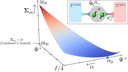
For thermodynamic efficiency, the reset protocol must be designed around the expected initial state. But what if the initial state is unknown, or expectations are misaligned? Fig. 1 illustrates the thermodynamic cost of misaligned expectations when the RESET operation is applied to two qubits that the protocol is not optimized for. This exposes the risk of divergent dissipation upon overspecialization—when the protocol operates on a state that is nearly orthogonal to the anticipated initial state $\sigma_{0}$.

For energetic efficiency in multiple use cases—say in resetting unknown qubits of a quantum computer—it is advisable when constructing such protocols to hedge thermodynamic bets. Bringing $\sigma_{0}$ closer to the fully mixed state (proportional to the identity) assures that no state is orthogonal to it.

V.3 Thermodynamic Cost of Modularity

Just as we break a classical circuit into elementary logic gates, building complex quantum operations generally involves decomposing them into elementary operations on smaller subsystems. The advantage of this modular design is that such elementary operations can then be mass produced, and then arranged to perform any number of desired complex tasks. Our main result implies that this modularity also incurs a thermodynamic price. Notably, each elementary operation must be optimized individually, without prior knowledge of where they’ll be placed in the grander scale. Accordingly, a mismatch is expected between the optimal vs. actual inputs, and dissipation is often unavoidable.

Consider a collection of elementary quantum operations $G_{n}$, acting on respective Hilbert space $\mathcal{H}_{n}$. Each is at-best individually optimized, such that dissipation is minimized for some $\sigma_{0,n}$. Suppose we place them in parallel to build a composite $N$-partite operation $\bigotimes_{n=1}^{N}G_{n}$. Individual optimization implies that the minimally dissipative state, $\sigma_{0}=\bigotimes_{n=1}^{N}\sigma_{0,n}$ will take a product form. Each reduced state $\rho_{0,n}$ input to the elementary operation $G_{n}$ may produce some mismatch dissipation if $\rho_{0,n}\neq\sigma_{0,n}$. Moreover, if the input to our computation, $\rho_{0}$, has correlations, we will incur additional dissipation from any lost correlation:

$$\tfrac{1}{k_{\text{B}}}\bigl{(}\bm{\Sigma}_{\rho_{0}}-\bm{\Sigma}_{\otimes_{n}\rho_{0,n}}\bigr{)}=-\Delta\text{D}\bigl{[}\rho_{t}\big{\|}\bigotimes_{n=1}^{N}\rho_{t,n}\bigr{]}~{}.$$ (17)

(See App. K for details of the derivation.) When $N=2$, this corresponds to the change in quantum mutual information induced by $G_{1}\otimes G_{2}$  [44, 45, 46]. This quantity is relevant, for example, when correlations are destroyed through local measurements or local erasure protocols.

In contrast to previous approaches [44, 45, 46], our derivation of modularity dissipation is valid for any parallel computation occurring in finite time, regardless of the local free energies of the memory elements utilized.

Individual component optimization is further limited when these parallel operations are embedded in series—since gate placement in a larger circuit will almost invariably change the distribution of input states it will encounter. Thus, a complex composite circuit is very unlikely to reach Landauer’s limit.

VI Generalization to other optimization problems

Our main result appears superficially similar to a recent result by Kolchinsky et al. [47], which describes the initial-state dependence of nonequilibrium free energy gain. In Ref. [47], it was shown that the maximal nonequilibrium free energy gain $\Delta\mathcal{F}_{\chi_{t}}$ differs from the free energy gain from any initial state $\rho_{0}$ according to the contraction of relative entropy between the two states $\rho_{t}$ and $\chi_{t}$ over the course of the protocol:

$$\Delta\mathcal{F}_{\chi_{t}}-\Delta\mathcal{F}_{\rho_{t}}=k_{\text{B}}T\text{D}[\rho_{0}\|\chi_{0}]-k_{\text{B}}T\text{D}[\rho_{\tau}\|\chi_{\tau}]~{}.$$ (18)

The main results there and here are nevertheless distinct since the initial state that leads to maximal free energy gain is typically not the same as the initial state that leads to minimal dissipation. Yet the similarity of the two results suggests a more general overarching result. Indeed, we have found a general theorem that contains these results as important cases.

To investigate, how any quantity depends on the initial state of the system, presupposes an initial product state of the system and environment: $\rho_{0}^{\text{tot}}=\rho_{0}\otimes\rho_{0}^{\text{env}}$. Furthermore, suppose that the joint system and environment evolve according to some unitary time evolution, such that the reduced state at time $\tau$ is given by $\rho_{\tau}=\text{tr}_{\text{env}}\bigl{(}\mathcal{U}\rho_{0}\otimes\rho_{0}^{\text{env}}\mathcal{U}^{\dagger}\bigr{)}$.

Consider any real-valued functional of the initial density matrix:

$$f(\rho_{0})=a(\rho_{0})+\text{tr}\bigl{(}\rho_{0}\ln\rho_{0}-\rho_{\tau}\ln\rho_{\tau}\bigr{)}~{},$$ (19)

and its minimizer:

$$\alpha_{0}\in\text{argmin}_{\rho_{0}}f(\rho_{0})~{}.$$ (20)

Suppose that $a(\rho)$ is an affine function, such that it can be written as $a(\rho)=\ell(\rho)+c$, where $\ell(\rho)$ is a linear function of $\rho$ and $c$ is a constant.

Theorem 2.

If $a(\rho)$ is an affine function of $\rho$, and $\alpha_{0}\in\text{argmin}_{\rho_{0}}f(\rho_{0})$ has a trivial nullspace, then $f(\rho_{0})-f(\alpha_{0})=\text{D}\bigl{[}\rho_{0}\big{\|}\alpha_{0}\bigr{]}-\text{D}\bigl{[}\rho_{\tau}\big{\|}\alpha_{\tau}\bigr{]}$.

Our proof of this theorem, given in App. O, parallels the proof of Thm. 1. If $\alpha_{0}$ has a non-trivial nullspace, then Thm. 2 can be extended as done in App. E.

The classical limit of Thm. 2 is closely related to a result recently derived in Ref. [48, Thm. 1].

Our main result concerns entropy production: $f(\rho_{0})=\tfrac{1}{k_{\text{B}}}\bm{\Sigma}_{\rho_{0}}$, for which $a(\rho_{0})=\text{tr}(\rho_{0}^{\text{env}}\ln\bm{\pi}^{\text{env}})-\text{tr}\bigl{(}\text{tr}_{\text{sys}}(\mathcal{U}_{x_{0:\tau}}\rho_{0}\otimes\rho_{0}^{\text{env}}\mathcal{U}_{x_{0:\tau}}^{\dagger})\ln\bm{\pi}^{\text{env}}\bigr{)}$ is indeed an affine function with $c=\text{tr}(\rho_{0}^{\text{env}}\ln\bm{\pi}^{\text{env}})$.

Ref. [47] considers the (negative) change in nonequilibrium free energy $f(\rho_{0})=\beta\mathcal{F}_{\rho_{0}}-\beta\mathcal{F}_{\rho_{\tau}}$, for which $a(\rho_{0})=\beta\text{tr}(\rho_{0}H_{0})-\beta\text{tr}(\rho_{\tau}H_{\tau})$ is a linear function of $\rho_{0}$. (Note that the minimum of the decrease in nonequilibrium free energy is the maximum increase.) With this form of $a(\rho)$, Thm. (2) immediately yields Eq. (18).

Another possibility is obtained if we simply let $a(\rho)=0$. Then we find a new result about the initial-state dependence of entropy change:

$$\Delta S(\rho_{t})-\Delta S(\kappa_{t})=k_{\text{B}}\text{D}\bigl{[}\rho_{0}\big{\|}\kappa_{0}\bigr{]}-k_{\text{B}}\text{D}\bigl{[}\rho_{\tau}\big{\|}\kappa_{\tau}\bigr{]}~{},$$ (21)

where $\kappa_{0}\in\text{argmin}_{\rho_{0}}S(\rho_{\tau})-S(\rho_{0})$.

A simple example reveals that these optimization problems indeed have different solutions (i.e., different $\alpha_{0}$s). Consider a double-well energy landscape. The right well is raised in a very short duration $\tau$ in which the system cannot fully relax. The initial distribution that minimizes dissipation primarily occupies the left well. The initial distribution that maximizes free energy gain primarily occupies the right well.

VII Discussion

In Eqs. (7) and (11), we exactly quantify dissipation in finite-time transformations of open quantum systems, and identify new relationships among dissipation, correlation, and distinction. When a system begins in any state other than the minimally dissipative initial state, the extra dissipation is exactly the contraction of the quantum relative entropy between them over the duration of the control protocol—their loss of distinguishability.

This has immediate consequences for thermally efficient quantum information processing. Crucially, a quantum control protocol cannot generally be made thermodynamically optimal for all possible input states, creating unavoidable dissipation beyond Landauer’s in quantum state preparation. Meanwhile, it imposes extra thermodynamic cost to modular computing architectures, where one wishes to optimize the thermal efficiency of certain quantum operations without pre-knowledge of how they will fit within a composite quantum protocol.

Our results are relevant for both quantum and classical finite-time thermodynamics. In the quantum regime, we have shown that the loss of coherence on the minimally dissipative eigenbasis directly contributes to dissipation. Appendix L further considers decoherence, and shows how our results quantify dissipation associated with non-selective measurement. Other applications of our finite-time equalities for nonequilibrium thermodynamics remain to be explored. For example, App. M suggests that our results may be leveraged to analyze dissipation in relaxation to nonequilibrium steady states.

Our general framework has allowed the investigation of entropy production’s dependence on initial conditions, even beyond the domain of the Second Law’s applicability. The role of system–environment correlation and nonequilibrium baths was highlighted in Eq. (7). The initial properties of the system itself were then shown to have many important consequences, through the implications of Eq. (11). From a broad philosophical perspective, these lessons extend our understanding of effective irreversibility in quantum mechanics, despite its global unitarity. More specifically, we have found how energetic resources are taxed for coherence, correlations, and misaligned expectations.

Appendix A Information-theoretic equalities for entropy production when the system begins correlated with nonequilibrium environments

Here, we derive new information-theoretic equalities (Eqs. (6) and (7)) for entropy production in the general case that allows for arbitrary initial correlation between the system and nonequilibrium environments. This generalizes a number of related results [19, 30, 20, 28, 31, 18].

Our result follows from the definition of entropy production together with the assumption of partially controlled unitary time evolution of the joint system and environment. Recall that entropy production is defined as

$$\bm{\Sigma}_{\rho_{0}}\equiv\bm{\Phi}+\Delta S(\rho_{t})~{},$$ (22)

with

$$\Delta S(\rho_{t})=k_{\text{B}}\text{tr}(\rho_{0}\ln\rho_{0})-k_{\text{B}}\text{tr}(\rho_{\tau}\ln\rho_{\tau})$$ (23)

and

$$\bm{\Phi}\equiv k_{\text{B}}\text{tr}(\rho_{0}^{\text{env}}\ln\bm{\pi}^{\text{env}})-k_{\text{B}}\text{tr}(\rho_{\tau}^{\text{env}}\ln\bm{\pi}^{\text{env}})~{}.$$ (24)

Notably, the assumption of joint unitary dynamics

$$\rho_{\tau}^{\text{tot}}=\mathcal{U}_{x_{0:\tau}}\rho_{0}^{\text{tot}}\mathcal{U}_{x_{0:\tau}}^{\dagger}~{},$$ (25)

guarantees that the net von Neumann entropy of the system and baths remains unchanged by the protocol:

$$\Delta S(\rho_{t}^{\text{tot}})=0~{}.$$ (26)

Recall that in general, the joint entropy between system and environment can be decomposed as

$$S(\rho_{t}^{\text{tot}})=S(\rho_{t})+S(\rho_{t}^{\text{env}})-k_{\text{B}}\mathcal{I}(\rho_{t};\rho_{t}^{\text{env}})~{}.$$ (27)

Combining this decomposition with Eq. (26), we find

$$\Delta S(\rho_{t}^{\text{tot}})=\Delta S(\rho_{t})+\Delta S(\rho_{t}^{\text{env}})-k_{\text{B}}\Delta\mathcal{I}(\rho_{t};\rho_{t}^{\text{env}})=0~{},$$ (28)

which can be rearranged as

$$\Delta S(\rho_{t})=-\Delta S(\rho_{t}^{\text{env}})+k_{\text{B}}\Delta\mathcal{I}(\rho_{t};\rho_{t}^{\text{env}})~{}.$$ (29)

Combining Eqs. (22) and (29), we find that

$$\tfrac{1}{k_{\text{B}}}\bm{\Sigma}_{\rho_{0}}=k_{\text{B}}\Delta\mathcal{I}(\rho_{t};\rho_{t}^{\text{env}})+\bm{\Phi}-\Delta S(\rho_{t}^{\text{env}})~{}.$$ (30)

Now combining Eqs. (30) and (24), we obtain

$$\bm{\Sigma}_{\rho_{0}}=\Delta\mathcal{I}(\rho_{t};\rho_{t}^{\text{env}})+\Delta\text{D}[\rho_{t}^{\text{env}}\|\bm{\pi}^{\text{env}}]~{}.$$ (31)

By the non-negativity of entropy, relative entropy, and mutual information, Eq. (31) provides a number of new bounds on entropy production and entropy flow that generalize both the Second Law of Thermodynamics and Landauer’s bound.

Initial correlation between system and environment can be thought of informally as catching a Maxwellian demon mid act, after correlation has already been established. To bring about correlation requires resources but, if it is already present, correlation can be consumed to reduce entropy production. Similarly, initially nonequilibrium environments can act as thermodynamic resources to reduce entropy production.

Alternatively, Maxwell’s demons can be accounted for within the standard framework of the Second Law by including the demon and ‘system under study’ as two subsystems of a larger system embedded in an initially equilibrium environment (which is, furthermore, initially uncorrelated with the two subsystems) [49, 50, 45]. But our generalized equality for entropy production allows for the boundaries between system and environment to be drawn arbitrarily, and thus describes entropy production (as a function of those chosen boundaries) in a broader set of scenarios.

The consequences of initial correlation or initially nonequilibrium environment can be quite astonishing. For example, either feature allows for heat to reliably flow from hot to cold reservoirs, as in Ref. [31].

Because of the product structure of the local-equilibrium reference state, Eq. (31) can be rewritten as

$$\bm{\Sigma}_{\rho_{0}} =\Delta S(\rho_{t})-\Delta\text{tr}(\rho_{t}^{\text{env}}\ln\bm{\pi}^{\text{env}})$$ (32)

$$=\Delta S(\rho_{t})+\sum_{b\in\mathbb{B}}-\Delta\text{tr}(\rho_{t}^{(b)}\ln\bm{\pi}^{(b)})$$ (33)

$$=\Bigl{[}\Delta S(\rho_{t})+\sum_{b\in\mathbb{B}}\Delta S(\rho_{t}^{(b)})\Bigr{]}+\sum_{b\in\mathbb{B}}\Delta\text{D}[\rho_{t}^{(b)}\|\bm{\pi}^{(b)}]$$ (34)

$$=\Delta\mathcal{T}_{t}+\sum_{b\in\mathbb{B}}\Delta\text{D}[\rho_{t}^{(b)}\|\bm{\pi}^{(b)}]~{},$$ (35)

where $\mathcal{T}_{t}=\text{D}\bigl{[}\rho_{t}^{\text{tot}}\big{\|}\rho_{t}\otimes\bigl{(}\bigotimes_{b\in\mathbb{B}}\rho_{t}^{(b)}\bigr{)}\bigr{]}$ is the total correlation among system and baths. (Here and throughout, $\rho_{t}^{(b)}=\text{tr}_{\text{sys},\mathbb{B}\setminus b}(\rho_{t}^{\text{tot}})$ is the reduced state of bath $b$ at time $t$.) This allows the perspective that entropy production is the change in the nonequilibrium addition to free energy of each bath, plus the change in total correlation among the system and all baths. Ref. [19, Eq. (17)] attained a special case of this result, under the assumption that the baths are initially in equilibrium and uncorrelated from the system and from each other. Our generalization allows rigorous consideration of much broader phenomena, in the presence of initial correlation with and between any nonequilibrium baths.

Appendix B Decompositions and interpretations of entropy flow

As will be made clear in the following, the expected value of entropy flow can generically be written as $\bm{\Phi}=-\Delta\text{tr}(\rho_{t}^{\text{env}}\ln\bm{\pi}^{\text{env}})$. By adding and subtracting the change in von Neumann entropy of the environment, this can be rewritten as

$$\bm{\Phi} =\Delta S(\rho_{t}^{\text{env}})+k_{\text{B}}\Delta\text{D}[\rho_{t}^{\text{env}}\|\bm{\pi}^{\text{env}}]~{}.$$ (36)

Recall that $\bm{\pi}^{\text{env}}=\bigotimes_{b\in\mathbb{B}}\bm{\pi}^{(b)}$, where $\bm{\pi}^{(b)}$ is the reference equilibrium state of bath $b$. Using the mathematical fact that $\text{tr}[\rho^{\prime}\ln(\rho_{A}\otimes\rho_{B})]=\text{tr}[\text{tr}_{\mathcal{H}_{B}}(\rho^{\prime})\ln(\rho_{A})]+\text{tr}[\text{tr}_{\mathcal{H}_{A}}(\rho^{\prime})\ln(\rho_{B})]$, we can alternatively decompose the entropy flow into the contributions from each bath. We will denote the reduced state of bath $b$ at time $t$ as: $\rho_{t}^{(b)}=\text{tr}_{\text{sys},\mathbb{B}\setminus b}(\rho_{t}^{\text{tot}})$. It then follows that

$$\bm{\Phi} =k_{\text{B}}\text{tr}(\rho_{0}^{\text{env}}\ln\bm{\pi}^{\text{env}})-k_{\text{B}}\text{tr}(\rho_{\tau}^{\text{env}}\ln\bm{\pi}^{\text{env}})$$ (37)

$$=k_{\text{B}}\sum_{b}\bigl{(}\text{tr}(\rho_{0}^{(b)}\ln\bm{\pi}^{(b)})-\text{tr}(\rho_{\tau}^{(b)}\ln\bm{\pi}^{(b)})\bigr{)}$$ (38)

$$=\sum_{b}\Delta S(\rho_{t}^{(b)})+k_{\text{B}}\Delta\text{D}[\rho_{\tau}^{(b)}\|\bm{\pi}^{(b)}]~{},$$ (39)

I.e., Entropy flow is the change in von Neumann entropy of the baths, plus the additional nonequilibrium free energy $k_{\text{B}}\Delta\text{D}[\rho_{t}^{(b)}\|\bm{\pi}^{(b)}]$ gained by each bath. Eq. (39) generalizes other decompositions of the entropy flow presented in Refs. [20, 28], which are obtained upon assumption of initially equilibrium baths that are uncorrelated with each other and with the system. Either Eq. (38) or Eq. (39) can be taken as the general definition of entropy flow, which allows our results to apply to baths from any thermodynamic ensemble [27].

Entropy flow has been of primary interest since the origins of thermodynamics. In its simplest form, when there is a single thermodynamic bath that a system can exchange energy with, entropy flow takes the form of $\frac{\text{heat flow to bath}}{\text{temperature of bath}}$. In quasistatic reversible transformations of an equilibrium system, this entropy flow will be equal to the change in equilibrium entropy of the system. However, for general irreversible transformations, the Second Law tells us that the entropy flow exceeds the change in system entropy. (Our results, however, caution us that this interpretation of the Second Law can be broken when initial correlations with the environment or the initial nonequilibrium nature of the environment are leveraged.)

More generally, we may consider entropy flow among many thermodynamic baths of any thermodynamic potentials. For example, baths of different temperatures may be introduced. Furthermore, chemical potentials and other coarse features of each bath may be incorporated into its thermodynamic potential [27].

As an important example, suppose each bath has a grand canonical reference state, such that

$$\bm{\pi}^{(b)}=e^{-\tfrac{1}{k_{\text{B}}T^{(b)}}\bigl{(}H^{(b)}-\sum_{\ell}\mu^{(b,\ell)}N^{(b,\ell)}\bigr{)}}/\mathcal{Z}^{(b)}~{},$$ (40)

where $T^{(b)}$ is the initial temperature of the $b^{\text{th}}$ bath, $H^{(b)}$ is its Hamiltonian, $\mu_{\ell}^{(b)}$ and $N_{\ell}^{(b)}$ are the initial chemical potential and the number operator for the bath’s $\ell^{\text{th}}$ particle type, and $\mathcal{Z}^{(b)}$ is the grand canonical partition function for the bath [26]. Even if the bath is not initially in equilibrium, the initial temperature and initial chemical potentials are well defined in statistical mechanics via average energy and expected particle number respectively. In particular, coarse “macroscopic” knowledge about total energy, particle numbers, etc. gives exactly the correct number of equations to solve for temperature, chemical potentials, etc. In the grand canonical case, initial temperature and chemical potentials are fixed by requiring that the equilibrium state shares the same expected energy, $\text{tr}(\bm{\pi}^{(b)}H^{(b)})=\text{tr}(\rho_{0}^{(b)}H^{(b)})$, and particle numbers, $\text{tr}(\bm{\pi}^{(b)}N^{(b,\ell)})=\text{tr}(\rho_{0}^{(b)}N^{(b,\ell)})$, as the actual initial state of the bath.

We can now use Eq. (38) to rewrite the entropy flow in the case of grand canonical reference states for the bath. First, we note that

$$-k_{\text{B}}\ln\bm{\pi}^{(b)}=-k_{\text{B}}\ln(\mathcal{Z}^{(b)})+\frac{H^{(b)}}{T^{(b)}}-\frac{1}{T^{(b)}}\sum_{\ell}\mu^{(b,\ell)}N^{(b,\ell)}~{}.$$ (41)

Accordingly, the expected change in this observable is

$$-k_{\text{B}}\Delta\text{tr}(\rho_{t}^{(b)}\ln\bm{\pi}^{(b)})=\frac{\Delta\text{tr}(\rho_{t}^{(b)}H^{(b)})}{T^{(b)}}-\frac{1}{T^{(b)}}\sum_{\ell}\mu^{(b,\ell)}\Delta\text{tr}(\rho_{t}^{(b)}N^{(b,\ell)})~{}.$$ (42)

Eq. (38) then reduces to the familiar form [24, 25, 19, 28]:

$$\bm{\Phi}=\sum_{b\in\mathbb{B}}\frac{Q^{(b)}}{T^{(b)}}-\frac{1}{T^{(b)}}\sum_{\ell}\mu^{(b,\ell)}\Delta\braket{N^{(b,\ell)}}~{},$$ (43)

where the heat $Q^{(b)}=\Delta\text{tr}(\rho_{t}^{(b)}H^{(b)})$ is the expected energy change of bath $b$ over the course of the process and $\Delta\braket{N^{(b,\ell)}}=\Delta\text{tr}(\rho_{t}^{(b)}N^{(b,\ell)})$ is the expected change in the bath’s number of $\ell$-type particles. Eq. (43) has been used to explore entropy flow and entropy production even in the case of arbitrarily small baths [19, 28].

Appendix C Derivation of the Gradient

To vary the initial state of the system while holding the initial state of the environment fixed requires $\rho_{0}^{\text{tot}}=\rho_{0}\otimes\rho_{0}^{\text{env}}$. We can fully specify the initial state of the system as $\rho_{0}=\sum_{j,k}c_{j,k}\ket{j}\bra{k}$. From Eqs. (2) through (4) of the main text, we can then express the entropy production as

$$\tfrac{1}{k_{\text{B}}}\bm{\Sigma}_{\rho_{0}} =\text{tr}(\rho_{0}\ln\rho_{0})-\text{tr}(\rho_{\tau}\ln\rho_{\tau})+\text{tr}(\rho_{0}^{\text{env}}\ln\bm{\pi}^{\text{env}})-\text{tr}\bigl{(}\text{tr}_{\text{sys}}(\mathcal{U}_{x_{0:\tau}}\rho_{0}\otimes\rho_{0}^{\text{env}}\mathcal{U}_{x_{0:\tau}}^{\dagger})\ln\bm{\pi}^{\text{env}}\bigr{)}$$ (44)

$$=\Bigl{(}\!\sum_{\lambda_{0}\in\Lambda_{\rho_{0}}}\!\!\lambda_{0}\ln\lambda_{0}\Bigr{)}-\Bigl{(}\!\sum_{\lambda_{\tau}\in\Lambda_{\rho_{\tau}}}\!\!\lambda_{\tau}\ln\lambda_{\tau}\Bigr{)}+\text{tr}(\rho_{0}^{\text{env}}\ln\bm{\pi}^{\text{env}})-\sum_{j,k}c_{j,k}\text{tr}\bigl{(}\text{tr}_{\text{sys}}(\mathcal{U}_{x_{0:\tau}}\ket{j}\bra{k}\otimes\rho_{0}^{\text{env}}\mathcal{U}_{x_{0:\tau}}^{\dagger})\ln\bm{\pi}^{\text{env}}\bigr{)}~{}.$$ (45)

Varying a single parameter $c_{j,k}$ of the initial density matrix yields the partial derivative:

$$\tfrac{1}{k_{\text{B}}}\frac{\partial}{\partial c_{j,k}}\bm{\Sigma}_{\rho_{0}} =\Bigl{(}\!\!\!\sum_{\lambda_{0}\in\Lambda_{\rho_{0}}}\!\!\Bigl{(}\frac{\partial\lambda_{0}}{\partial c_{j,k}}\Bigr{)}\ln\lambda_{0}+\frac{\partial\lambda_{0}}{\partial c_{j,k}}\Bigr{)}-\Bigl{(}\!\!\!\sum_{\lambda_{\tau}\in\Lambda_{\rho_{\tau}}}\!\!\Bigl{(}\frac{\partial\lambda_{\tau}}{\partial c_{j,k}}\Bigr{)}\ln\lambda_{\tau}+\frac{\partial\lambda_{\tau}}{\partial c_{j,k}}\Bigr{)}-\text{tr}\bigl{(}\text{tr}_{\text{sys}}(\mathcal{U}_{x_{0:\tau}}\!\ket{j}\!\bra{k}\otimes\rho_{0}^{\text{env}}\mathcal{U}_{x_{0:\tau}}^{\dagger})\ln\bm{\pi}^{\text{env}}\bigr{)}$$

which leads us to evaluate the infinitesimal perturbations $\frac{\partial\lambda_{0}}{\partial c_{j,k}}$ and $\frac{\partial\lambda_{\tau}}{\partial c_{j,k}}$ to the eigenvalues of $\rho_{0}$ and $\rho_{\tau}$ respectively.

(We could alternatively choose to vary real-valued variables $c_{j,k}^{(\text{r})}$ and $c_{j,k}^{(i)}$, such that $c_{j,k}^{(\text{r})}=\tfrac{1}{2}(c_{j,k}+c_{k,j})$ and $c_{j,k}^{(i)}=\tfrac{-i}{2}(c_{j,k}-c_{k,j})$. Then we can write $\rho_{0}=\sum_{j,k}(c_{j,k}^{(\text{r})}+ic_{j,k}^{(i)})\ket{j}\bra{k}$ and differentiate with respect to these real variables. However, it conveniently turns out that $\bm{\Sigma}_{\rho_{0}}$ is complex-differentiable in all complex-valued $c_{j,k}$ variables, so we can differentiate directly with respect to $c_{j,k}$.)

Starting with the eigen-relation: $\rho_{0}\ket{\lambda_{0}}=\lambda_{0}\ket{\lambda_{0}}$, we can take the partial derivative of each side:

$$\frac{\partial}{\partial c_{j,k}}\rho_{0}\ket{\lambda_{0}} =\Bigl{(}\frac{\partial}{\partial c_{j,k}}\rho_{0}\Bigr{)}\ket{\lambda_{0}}+\rho_{0}\frac{\partial}{\partial c_{j,k}}\ket{\lambda_{0}}\qquad=\qquad\frac{\partial}{\partial c_{j,k}}\lambda_{0}\ket{\lambda_{0}}=\Bigl{(}\frac{\partial\lambda_{0}}{\partial c_{j,k}}\Bigr{)}\ket{\lambda_{0}}+\lambda_{0}\frac{\partial}{\partial c_{j,k}}\ket{\lambda_{0}}~{}.$$ (46)

Left-multiplying by $\bra{\lambda_{0}}$, and recalling that $\rho_{0}=\sum_{j,k}c_{j,k}\ket{j}\bra{k}$, we obtain

$$\Bigl{(}\frac{\partial\lambda_{0}}{\partial c_{j,k}}\Bigr{)}\braket{\lambda_{0}}{\lambda_{0}}=\frac{\partial\lambda_{0}}{\partial c_{j,k}}=\bra{\lambda_{0}}\Bigl{(}\underbrace{\frac{\partial}{\partial c_{j,k}}\rho_{0}}_{\ket{j}\bra{k}}\Bigr{)}\ket{\lambda_{0}}+\underbrace{\underbrace{\bra{\lambda_{0}}\rho_{0}\frac{\partial}{\partial c_{j,k}}\ket{\lambda_{0}}}_{=\lambda_{0}\bra{\lambda_{0}}\frac{\partial}{\partial c_{j,k}}\ket{\lambda_{0}}}-\lambda_{0}\bra{\lambda_{0}}\frac{\partial}{\partial c_{j,k}}\ket{\lambda_{0}}}_{=0}~{},$$ (47)

which yields

$$\frac{\partial\lambda_{0}}{\partial c_{j,k}}=\braket{\lambda_{0}}{j}\braket{k}{\lambda_{0}}=\braket{k}{\lambda_{0}}\braket{\lambda_{0}}{j}~{}.$$ (48)

The summations over $\lambda_{0}$ thus become

$$\sum_{\lambda_{0}\in\Lambda_{\rho_{0}}}\frac{\partial\lambda_{0}}{\partial c_{j,k}} =\sum_{\lambda_{0}\in\Lambda_{\rho_{0}}}\braket{k}{\lambda_{0}}\braket{\lambda_{0}}{j}=\bra{k}\Bigl{(}\underbrace{\sum_{\lambda_{0}\in\Lambda_{\rho_{0}}}\ket{\lambda_{0}}\bra{\lambda_{0}}}_{=I}\Bigr{)}\ket{j}=\braket{k}{j}=\text{tr}\bigl{(}\ket{j}\bra{k}\bigr{)}$$ (49)

and

$$\sum_{\lambda_{0}\in\Lambda_{\rho_{0}}}\Bigl{(}\frac{\partial\lambda_{0}}{\partial c_{j,k}}\Bigr{)}\ln\lambda_{0} =\sum_{\lambda_{0}\in\Lambda_{\rho_{0}}}\braket{k}{\lambda_{0}}\braket{\lambda_{0}}{j}\ln\lambda_{0}=\bra{k}\Bigl{(}\underbrace{\sum_{\lambda_{0}\in\Lambda_{\rho_{0}}}\ln\lambda_{0}\ket{\lambda_{0}}\bra{\lambda_{0}}}_{=\ln\rho_{0}}\Bigr{)}\ket{j}=\braket{k}{\ln\rho_{0}}{j}=\text{tr}\bigl{(}\ket{j}\bra{k}\ln\rho_{0}\bigr{)}~{}.$$ (50)

Moving on to the slightly more involved perturbation, we use the eigen-relation: $\rho_{\tau}\ket{\lambda_{\tau}}=\lambda_{\tau}\ket{\lambda_{\tau}}$ and again take the partial derivative of each side:

$$\frac{\partial}{\partial c_{j,k}}\rho_{\tau}\ket{\lambda_{\tau}} =\Bigl{(}\frac{\partial}{\partial c_{j,k}}\rho_{\tau}\Bigr{)}\ket{\lambda_{\tau}}+\rho_{\tau}\frac{\partial}{\partial c_{j,k}}\ket{\lambda_{\tau}}\qquad=\qquad\frac{\partial}{\partial c_{j,k}}\lambda_{\tau}\ket{\lambda_{\tau}}=\Bigl{(}\frac{\partial\lambda_{\tau}}{\partial c_{j,k}}\Bigr{)}\ket{\lambda_{\tau}}+\lambda_{\tau}\frac{\partial}{\partial c_{j,k}}\ket{\lambda_{\tau}}~{}.$$ (51)

Left-multiplying by $\bra{\lambda_{\tau}}$, and recalling that $\rho_{\tau}=\sum_{j,k}c_{j,k}\text{tr}_{\text{env}}\bigl{(}\mathcal{U}_{x_{0:\tau}}\ket{j}\bra{k}\otimes\rho_{0}^{\text{env}}\mathcal{U}_{x_{0:\tau}}^{\dagger}\bigr{)}$, we obtain

$$\Bigl{(}\frac{\partial\lambda_{\tau}}{\partial c_{j,k}}\Bigr{)}\braket{\lambda_{\tau}}{\lambda_{\tau}}=\frac{\partial\lambda_{\tau}}{\partial c_{j,k}}=\bra{\lambda_{\tau}}\Bigl{(}\!\!\!\!\!\!\!\!\!\!\underbrace{\frac{\partial}{\partial c_{j,k}}\rho_{\tau}}_{\text{tr}_{\text{env}}\bigl{(}\mathcal{U}_{x_{0:\tau}}\ket{j}\bra{k}\otimes\rho_{0}^{\text{env}}\mathcal{U}_{x_{0:\tau}}^{\dagger}\bigr{)}}\!\!\!\!\!\!\!\!\!\!\Bigr{)}\ket{\lambda_{\tau}}+\underbrace{\underbrace{\bra{\lambda_{\tau}}\rho_{\tau}\frac{\partial}{\partial c_{j,k}}\ket{\lambda_{\tau}}}_{=\lambda_{\tau}\bra{\lambda_{\tau}}\frac{\partial}{\partial c_{j,k}}\ket{\lambda_{\tau}}}-\lambda_{\tau}\bra{\lambda_{\tau}}\frac{\partial}{\partial c_{j,k}}\ket{\lambda_{\tau}}}_{=0}~{},$$ (52)

which yields

$$\frac{\partial\lambda_{\tau}}{\partial c_{j,k}}=\braket{\lambda_{\tau}}{\text{tr}_{\text{env}}\bigl{(}\mathcal{U}_{x_{0:\tau}}\ket{j}\bra{k}\otimes\rho_{0}^{\text{env}}\mathcal{U}_{x_{0:\tau}}^{\dagger}\bigr{)}}{\lambda_{\tau}}~{}.$$ (53)

The summations over $\lambda_{\tau}$ thus become

$$\sum_{\lambda_{\tau}\in\Lambda_{\rho_{\tau}}}\frac{\partial\lambda_{\tau}}{\partial c_{j,k}} =\sum_{\lambda_{\tau}\in\Lambda_{\rho_{\tau}}}\braket{\lambda_{\tau}}{\text{tr}_{\text{env}}\bigl{(}\mathcal{U}_{x_{0:\tau}}\ket{j}\bra{k}\otimes\rho_{0}^{\text{env}}\mathcal{U}_{x_{0:\tau}}^{\dagger}\bigr{)}}{\lambda_{\tau}}=\text{tr}\Bigl{(}\text{tr}_{\text{env}}\bigl{(}\mathcal{U}_{x_{0:\tau}}\ket{j}\bra{k}\otimes\rho_{0}^{\text{env}}\mathcal{U}_{x_{0:\tau}}^{\dagger}\bigr{)}\Bigr{)}$$ (54)

$$=\text{tr}\bigl{(}\mathcal{U}_{x_{0:\tau}}\ket{j}\bra{k}\otimes\rho_{0}^{\text{env}}\mathcal{U}_{x_{0:\tau}}^{\dagger}\bigr{)}=\text{tr}\bigl{(}\ket{j}\bra{k}\otimes\rho_{0}^{\text{env}}\bigr{)}=\text{tr}\bigl{(}\ket{j}\bra{k}\bigr{)}$$ (55)

and

$$\sum_{\lambda_{\tau}\in\Lambda_{\rho_{\tau}}}\Bigl{(}\frac{\partial\lambda_{\tau}}{\partial c_{j,k}}\Bigr{)}\ln\lambda_{\tau} =\sum_{\lambda_{\tau}\in\Lambda_{\rho_{\tau}}}\braket{\lambda_{\tau}}{\text{tr}_{\text{env}}\bigl{(}\mathcal{U}_{x_{0:\tau}}\ket{j}\bra{k}\otimes\rho_{0}^{\text{env}}\mathcal{U}_{x_{0:\tau}}^{\dagger}\bigr{)}}{\lambda_{\tau}}\ln\lambda_{\tau}$$ (56)

$$=\text{tr}\biggl{(}\Bigl{(}\underbrace{\sum_{\lambda_{\tau}\in\Lambda_{\rho_{\tau}}}\ln\lambda_{\tau}\ket{\lambda_{\tau}}\bra{\lambda_{\tau}}}_{=\ln\rho_{\tau}}\Bigr{)}\text{tr}_{\text{env}}\bigl{(}\mathcal{U}_{x_{0:\tau}}\ket{j}\bra{k}\otimes\rho_{0}^{\text{env}}\mathcal{U}_{x_{0:\tau}}^{\dagger}\bigr{)}\biggr{)}$$ (57)

$$=\text{tr}\Bigl{(}\text{tr}_{\text{env}}\bigl{(}\mathcal{U}_{x_{0:\tau}}\ket{j}\bra{k}\otimes\rho_{0}^{\text{env}}\mathcal{U}_{x_{0:\tau}}^{\dagger}\bigr{)}\ln\rho_{\tau}\Bigr{)}~{}.$$ (58)

Plugging in our new expressions for the $\lambda_{0}$ an $\lambda_{\tau}$ summations in Eqs. (49), (50), (55), and (58), we obtain

$$\tfrac{1}{k_{\text{B}}}\frac{\partial}{\partial c_{j,k}}\bm{\Sigma}_{\rho_{0}} =\Bigl{(}\!\!\!\sum_{\lambda_{0}\in\Lambda_{\rho_{0}}}\!\!\Bigl{(}\frac{\partial\lambda_{0}}{\partial c_{j,k}}\Bigr{)}\ln\lambda_{0}+\frac{\partial\lambda_{0}}{\partial c_{j,k}}\Bigr{)}-\Bigl{(}\!\!\!\sum_{\lambda_{\tau}\in\Lambda_{\rho_{\tau}}}\!\!\Bigl{(}\frac{\partial\lambda_{\tau}}{\partial c_{j,k}}\Bigr{)}\ln\lambda_{\tau}+\frac{\partial\lambda_{\tau}}{\partial c_{j,k}}\Bigr{)}-\text{tr}\bigl{(}\text{tr}_{\text{sys}}(\mathcal{U}_{x_{0:\tau}}\!\ket{j}\!\bra{k}\otimes\rho_{0}^{\text{env}}\mathcal{U}_{x_{0:\tau}}^{\dagger})\ln\bm{\pi}^{\text{env}}\bigr{)}$$

$$=\text{tr}\bigl{(}\ket{j}\bra{k}\ln\rho_{0}\bigr{)}-\text{tr}\Bigl{(}\text{tr}_{\text{env}}\bigl{(}\mathcal{U}_{x_{0:\tau}}\ket{j}\bra{k}\otimes\rho_{0}^{\text{env}}\mathcal{U}_{x_{0:\tau}}^{\dagger}\bigr{)}\ln\rho_{\tau}\Bigr{)}-\text{tr}\Bigl{(}\text{tr}_{\text{sys}}\bigl{(}\mathcal{U}_{x_{0:\tau}}\ket{j}\bra{k}\otimes\rho_{0}^{\text{env}}\mathcal{U}_{x_{0:\tau}}^{\dagger}\bigr{)}\ln\bm{\pi}^{\text{env}}\Bigr{)}~{}.$$ (59)

Recall that we have introduced a gradient $\bm{\nabla}\bm{\Sigma}_{\rho_{0}}\equiv\sum_{j,k}\ket{k}\bra{j}\frac{\partial}{\partial c_{j,k}}\bm{\Sigma}_{\rho_{0}}$ and a scalar product $\gamma\cdot\bm{\nabla}\bm{\Sigma}_{\rho_{0}}\equiv\text{tr}(\gamma\bm{\nabla}\bm{\Sigma}_{\rho_{0}})$.

This allows us to inspect local changes in entropy production $(\rho_{0}-\rho_{0}^{\prime})\cdot\bm{\nabla}\bm{\Sigma}_{\rho_{0}^{\prime}}$ as we move from $\rho_{0}^{\prime}$ towards any other density matrix $\rho_{0}$. By the convexity of quantum states, there is indeed a continuum of density matrices in this direction; so the sign of the directional derivative indeed indicates the sign of the change in entropy production for infinitesimal changes to the initial density matrix in the direction of $\rho_{0}$.

For any two density matrices $\rho_{0}=\sum_{j,k}c_{j,k}\ket{j}\!\bra{k}$ and $\rho_{0}^{\prime}=\sum_{j,k}c_{j,k}^{\prime}\ket{j}\!\bra{k}$, Eq. (59) implies that

$$\tfrac{1}{k_{\text{B}}}\rho_{0}\cdot\!\bm{\nabla}\bm{\Sigma}_{\rho_{0}^{\prime}} =\tfrac{1}{k_{\text{B}}}\text{tr}(\rho_{0}\bm{\nabla}\bm{\Sigma}_{\rho_{0}^{\prime}})$$ (60)

$$=\tfrac{1}{k_{\text{B}}}\sum_{j,k}c_{j,k}\frac{\partial}{\partial c_{j,k}^{\prime}}\bm{\Sigma}_{\rho_{0}^{\prime}}$$ (61)

$$=\text{tr}(\rho_{0}\ln\rho_{0}^{\prime})-\text{tr}(\rho_{\tau}\ln\rho_{\tau}^{\prime})-\text{tr}(\rho_{\tau}^{\text{env}}\ln\bm{\pi}^{\text{env}})~{}.$$ (62)

so that we arrive at Lem. 1 of the main text.

Appendix D Useful Lemmas

Here we derive useful lemmas about entropy production for arbitrary decompositions of the initial density matrix. We consider any set of component density matrices $\{\rho_{0}^{(n)}\}_{n}$ and corresponding probabilities $\{\Pr(n)\}_{n}$ such that $\rho_{0}=\sum_{n}\Pr(n)\rho_{0}^{(n)}$.

Lemma 2.

Dissipation is convex over initial density matrices.

Let $\rho_{0}=\sum_{n}\Pr(n)\rho_{0}^{(n)}$. Then:

$\displaystyle\Bigl{(}\sum_{n}\Pr(n)\bm{\Sigma}_{\rho_{0}^{(n)}}\Bigr{)}-\bm{\Sigma}_{\rho_{0}}$ $\displaystyle\;\,=\Bigl{[}S(\rho_{0})-\sum_{n}\Pr(n)S(\rho_{0}^{(n)})\Bigr{]}-\Bigl{[}S(\rho_{\tau})-\sum_{n}\Pr(n)S(\rho_{\tau}^{(n)})\Bigr{]}$ (63) $\displaystyle\;\,=\Bigl{[}\sum_{n}\Pr(n)\text{D}\bigl{[}\rho_{0}^{(n)}\big{\|}\rho_{0}\bigr{]}\Bigr{]}-\Bigl{[}\sum_{n}\Pr(n)\text{D}\bigl{[}\rho_{\tau}^{(n)}\big{\|}\rho_{\tau}\bigr{]}\Bigr{]}$ (64) $\displaystyle\;\,\geq 0~{}.$ (65)

Eq. (63) is obtained from the recognition that entropy flow $\bm{\Phi}$ is an affine function of $\rho_{0}$, and so cancels between $\bm{\Sigma}_{\rho_{0}}$ and $\sum_{n}\Pr(n)\bm{\Sigma}_{\rho_{0}^{(n)}}$. Each of the square brackets then represents a Holevo information, before and after the transformation, respectively. The non-negativity is finally obtained by the information processing inequality applied to the Holevo information. (Non-negativity can be seen to follow from each $n$ separately: I.e., $\text{D}\bigl{[}\rho_{0}^{(n)}\big{\|}\rho_{0}\bigr{]}\geq\text{D}\bigl{[}\rho_{\tau}^{(n)}\big{\|}\rho_{\tau}\bigr{]}$.)

Lemma 3.

Dissipation is linearly combined as $\bm{\Sigma}_{\rho_{0}}=\sum_{n}\Pr(n)\bm{\Sigma}_{\rho_{0}^{(n)}}$ if the elements of $\{\rho_{0}^{(n)}\}_{n}$ are mutually orthogonal and also the elements of $\{\rho_{\tau}^{(n)}\}_{n}$ are mutually orthogonal.

If $\rho_{t}^{(m)}$ and $\rho_{t}^{(n)}$ are orthogonal (i.e., $\text{tr}(\rho_{t}^{(m)}\rho_{t}^{(n)})=0$ when $m\neq n$), then they are simultaneously diagonalizable. If this orthogonality holds for all pairs in the set $\{\rho_{t}^{(n)}\}_{n}$, then the simultaneous diagonalizability implies that $\rho_{t}=\sum_{n}\Pr(n)\rho_{t}^{(n)}$ inherits the eigenvalues of $\rho_{t}^{(n)}$ multiplied by their respective $\Pr(n)$. I.e.: $\rho_{t}$’s spectrum is then

$$\Lambda_{\rho_{t}}=\bigcup_{n}\bigl{\{}\lambda\Pr(n):\lambda\in\Lambda_{\rho_{0}^{(n)}}\bigr{\}}~{},$$ (66)

with multiplicities inherited from the constituent spectra.

In this scenario, the von Neumann entropy cleaves into two pieces:

$$S(\rho_{t}) =-k_{\text{B}}\sum_{\zeta\in\Lambda_{\rho_{t}}}\zeta\ln\zeta$$ (67)

$$=-k_{\text{B}}\sum_{n}\sum_{\lambda\in\Lambda_{\rho_{t}^{(n)}}}\lambda\Pr(n)\ln\bigl{(}\lambda\Pr(n)\bigr{)}$$ (68)

$$=-k_{\text{B}}\Bigl{(}\sum_{n}\Pr(n)\sum_{\lambda\in\Lambda_{\rho_{t}^{(n)}}}\lambda\ln\lambda\Bigr{)}$$

$$\qquad-k_{\text{B}}\sum_{n}\Pr(n)\ln\bigl{(}\Pr(n)\bigr{)}\sum_{\lambda\in\Lambda_{\rho_{t}^{(n)}}}\lambda$$ (69)

$$=\Bigl{(}\sum_{n}\Pr(n)S(\rho_{0}^{(n)})\Bigr{)}-k_{\text{B}}\sum_{n}\Pr(n)\ln\bigl{(}\Pr(n)\bigr{)}~{},$$ (70)

where we used the fact that $\sum_{\lambda\in\Lambda_{\rho_{t}^{(n)}}}\lambda=1$. The difference in entropy then yields

$\displaystyle S(\rho_{0})-S(\rho_{\tau})$ $\displaystyle=\Bigl{(}\sum_{n}\Pr(n)S(\rho_{0}^{(n)})\Bigr{)}-\Bigl{(}\sum_{n}\Pr(n)S(\rho_{\tau}^{(n)})\Bigr{)}~{}.$ (71)

Together with Eq. (63), this implies that $\bm{\Sigma}_{\rho_{0}}=\sum_{n}\Pr(n)\bm{\Sigma}_{\rho_{0}^{(n)}}$, proving Lemma 3.

Appendix E Generalized $\sigma_{0}$ for non-interacting basins

It is possible that the evolution acts completely independently on distinct basins of state space. This will generically yield a nontrivial nullspace for $\text{argmin}_{\rho_{0}}\bm{\Sigma}_{\rho_{0}}$. In such cases, it is profitable to generalize the definition of $\sigma_{0}$ so that it includes the successive minimally dissipative density matrices that carve out the independent basins on the nullspace. These basins will be formally defined shortly.

We use the terminology ‘basin’ in analogy with ‘basins of attraction’ in nonlinear dynamics. Indeed, for certain dynamics that induce autonomous nonequilibrium steady states, this section addresses the quantum thermodynamics of coexisting basins of attraction for an open quantum system. However, this section more generally addresses non-autonomous dynamics, and allows for the possibility of thermodynamically independent regions of state space. When a basin is dissipative, our results imply that trajectories from the initial conditions inside it must become less distinguishable over time—they contract to a generalized time-dependent notion of attractor.

We will show that, within each basin, the extra dissipation due to a non-minimally dissipative initial density matrix is given exactly by the contraction of the relative entropy between the actual and minimally dissipative initial density matrices under the same driving $x_{0:\tau}$.

To make progress in this generalized setting, we must first introduce several new notions.

E.1 Definitions

Let $\mathcal{P}(\mathcal{H})$ be the set of density matrices that can be constructed on the Hilbert space $\mathcal{H}$. I.e., $\displaystyle\mathcal{P}(\mathcal{H})\equiv\Bigl{\{}\sum_{\ell}\Pr(\ell)\frac{\ket{\ell}\bra{\ell}}{\braket{\ell}{\ell}}:\ket{\ell}\in\mathcal{H}\!\setminus\!\{\vec{0}\},\,0\!<\!\Pr(\ell)\!\leq\!1,\text{ and }\sum_{\ell}\Pr(\ell)=1\Bigr{\}}.$ (72)

Let $\mathcal{H}^{\text{sys}}$ be the Hilbert space of the physical system under study (not including the environment). We will denote the nullspace of an operator $\rho$ as null$(\rho)$. I.e.: $\text{null}(\rho)=\bigl{\{}\ket{\eta}\in\mathcal{H}^{\text{sys}}:\rho\ket{\eta}=\vec{0}\bigr{\}}$. The ‘support’ of a density matrix is the space orthogonal to its nullspace.

We can now introduce the successive minimally dissipative density matrices $\{\sigma_{0}^{[n]}\}_{n}$. The absolute minimum dissipation is achieved via the minimally dissipative density matrix $\sigma_{0}^{[0]}$:

$$\sigma_{0}^{[0]}\in\text{argmin}_{\rho_{0}\in\mathcal{P}(\mathcal{H}^{\text{sys}})}\bm{\Sigma}_{\rho_{0}}~{}.$$ (73)

In the main text, where $\sigma_{0}^{[0]}$ has a trivial nullspace (of $\{\vec{0}\}$), we identified $\sigma_{0}^{[0]}$ with $\sigma_{0}$ itself. However, when $\sigma_{0}^{[0]}$ has a nontrivial nullspace, we will also want to consider the minimally dissipative density matrix on the nullspace: $\sigma_{0}^{[1]}\in\text{argmin}_{\rho_{0}\in\mathcal{P}\bigl{(}\text{null}(\sigma_{0}^{[0]})\bigr{)}}\bm{\Sigma}_{\rho_{0}}$. If $\sigma_{0}^{[1]}$ also has a nontrivial nullspace, then we continue in the same fashion to identify the minimally dissipative density matrix within the intersection of all of the preceding nullspaces. In general, the $n^{\text{th}}$ thermodynamically independent basin has the minimally dissipative initial state:

$$\sigma_{0}^{[n]}\in\text{argmin}_{\rho_{0}\in\mathcal{P}\bigl{(}\bigcap_{m=0}^{n-1}\text{null}(\sigma_{0}^{[m]})\bigr{)}}\bm{\Sigma}_{\rho_{0}}$$ (74)

for $n\geq 1$.

The $n^{\text{th}}$ minimally dissipative basin is the Hilbert space:

$$\mathcal{H}_{0}^{[n]}=\text{span}\Bigl{(}\bigl{\{}\ket{\lambda}:\lambda\in\Lambda_{\sigma_{0}^{[n]}}\setminus 0\bigr{\}}\Bigr{)}~{},$$ (75)

which is the support of $\sigma_{0}^{[n]}$. We call this space a ‘basin’ in loose analogy with the basins of attraction of classical nonlinear dynamics. We will employ the projector

$$\Pi_{\mathcal{H}_{0}^{[n]}}=\sum_{\lambda\in\Lambda_{\!\sigma_{0}^{[n]}}\setminus\{0\}}\frac{\ket{\lambda}\bra{\lambda}}{\braket{\lambda}{\lambda}}$$ (76)

which projects onto $\mathcal{H}_{0}^{[n]}$. Notably, these projectors constitute a decomposition of the identity $I$ on the system’s state space $\mathcal{H}^{\text{sys}}$:

$$\sum_{n}\Pi_{\mathcal{H}_{0}^{[n]}}=I~{}.$$ (77)

We can now define the minimally dissipative reference state $\sigma_{0}$, as if $\rho_{0}$ were minimally dissipative on each of the thermodynamically independent basins on which it lives:

$$\sigma_{0}\equiv\sum_{n}\text{tr}(\Pi_{\mathcal{H}_{0}^{[n]}}\rho_{0})\sigma_{0}^{[n]}~{}.$$ (78)

It should be noted that the $\rho_{0}$-dependence is only via the weight $\text{tr}(\Pi_{\mathcal{H}_{0}^{[n]}}\rho_{0})$ of $\rho_{0}$ on each thermodynamically-independent basin, used to linearly combine their contributions.

E.2 Generalized dissipation bound

With these definitions in place, let us now reconsider the task at hand.

If $\sigma_{0}^{[0]}$ has a nontrivial nullspace (and if $\bm{\Sigma}_{\rho_{0}}$ is finite for all $\rho_{0}$), then there are thermodynamically isolated basins of state-space. (The support of $\sigma_{0}^{[0]}$ is the minimally dissipative basin $\mathcal{H}_{0}^{[n]}$, which is a strict subset of $\mathcal{H}^{\text{sys}}$.) Then, since a generic initial state $\rho_{0}$ may have support on the nullspace of $\sigma_{0}^{[0]}$, Eq. (10) is no longer directly valid. However, for any two initial density matrices $\rho_{0}$ and $\xi_{0}$ such that the support of $\rho_{0}$ is a subset of the support of $\xi_{0}$, it is still true that

$$(\rho_{0}-\xi_{0})\cdot\bm{\nabla}\bm{\Sigma}_{\xi_{0}}$$

$$\quad=\bm{\Sigma}_{\rho_{0}}-\bm{\Sigma}_{\xi_{0}}-k_{\text{B}}\Bigl{(}\text{D}\bigl{[}\rho_{0}\big{\|}\xi_{0}\bigr{]}-\text{D}\bigl{[}\rho_{\tau}\big{\|}\xi_{\tau}\bigr{]}\Bigr{)}~{}.$$ (79)

Indeed $\sigma_{0}$, as defined in Eq. (78), is guaranteed to have support equal to $\mathcal{H}^{\text{sys}}$, and so Eq. (79) is valid if we set $\xi_{0}=\sigma_{0}$. Alternatively, we can set $\xi_{0}=\sigma_{0}^{[n]}$ if we properly restrict $\rho_{0}$.

To proceed, we recognize that $\rho_{0}$ can be decomposed via Eq. (77) as

$$\rho_{0} =\rho_{0}^{\Box}+\rho_{0}^{\text{coh}}~{},$$ (80)

where

$$\rho_{0}^{\Box} \equiv\sum_{n}\text{tr}(\Pi_{\mathcal{H}_{0}^{[n]}}\rho_{0})\rho_{0}^{[n]} \,\text{ with }\,\rho_{0}^{[n]}\equiv\frac{\Pi_{\mathcal{H}_{0}^{[n]}}\rho_{0}\Pi_{\mathcal{H}_{0}^{[n]}}}{\text{tr}(\Pi_{\mathcal{H}_{0}^{[n]}}\rho_{0})}$$

and

$$\rho_{0}^{\text{coh}} \equiv\sum_{m,n\atop m\neq n}\Pi_{\mathcal{H}_{0}^{[m]}}\rho_{0}\Pi_{\mathcal{H}_{0}^{[n]}}~{}.$$

$\rho_{0}^{\Box}$ projects $\rho_{0}$ onto the minimally dissipative basins, whereas $\rho_{0}^{\text{coh}}$ describes the state’s coherence between these basins.

Since $\sigma_{0}^{[n]}$ is, by definition, the minimally dissipative density matrix on its subspace (and, since it has full support on that subspace), we have that

$$0 =(\rho_{0}^{[n]}-\sigma_{0}^{[n]})\cdot\bm{\nabla}\bm{\Sigma}_{\sigma_{0}^{[n]}}$$ (81)

$$=\bm{\Sigma}_{\rho_{0}^{[n]}}-\bm{\Sigma}_{\sigma_{0}^{[n]}}-k_{\text{B}}\Bigl{(}\text{D}\bigl{[}\rho_{0}^{[n]}\big{\|}\sigma_{0}^{[n]}\bigr{]}-\text{D}\bigl{[}\rho_{\tau}^{[n]}\big{\|}\sigma_{\tau}^{[n]}\bigr{]}\Bigr{)}~{}.$$ (82)

As an immediate consequence of their definition, the elements of $\{\sigma_{0}^{[n]}\}_{n}$ are mutually orthogonal, and the elements of $\{\rho_{0}^{[n]}\}_{n}$ are mutually orthogonal. It is often the case (and, we conjecture, generally true) that the coexistence of these $\sigma_{0}^{[n]}$ basins implies the orthogonality of their evolved states. I.e., the elements of $\{\sigma_{\tau}^{[n]}\}_{n}$ are mutually orthogonal and the elements of $\{\rho_{\tau}^{[n]}\}_{n}$ are mutually orthogonal. Lemma 3 then implies that

$$\bm{\Sigma}_{\sigma_{0}}=\sum_{n}\text{tr}(\Pi_{\mathcal{H}_{0}^{[n]}}\rho_{0})\bm{\Sigma}_{\sigma_{0}^{[n]}}$$ (83)

and

$$\bm{\Sigma}_{\rho_{0}^{\Box}}=\sum_{n}\text{tr}(\Pi_{\mathcal{H}_{0}^{[n]}}\rho_{0})\bm{\Sigma}_{\rho_{0}^{[n]}}~{}.$$ (84)

Together with Eq. (82) this leads to

$$\bm{\Sigma}_{\rho_{0}^{\Box}}-\bm{\Sigma}_{\sigma_{0}} =k_{\text{B}}\Bigl{(}\text{D}\bigl{[}\rho_{0}^{\Box}\big{\|}\sigma_{0}\bigr{]}-\text{D}\bigl{[}\rho_{\tau}^{\Box}\big{\|}\sigma_{\tau}\bigr{]}\Bigr{)}~{}.$$ (85)

Eq. (85) can be seen as the quantum generalization of the classical result obtained recently in Ref. [48]. The classical version of this result is relevant when the minimally dissipative probability distribution ($\sigma_{0}^{[0]}$) does not have full support. Dissipation on other ‘islands’ are then considered. Our derivation points out the nuances of physical assumptions that go into the classical result, and refines the notion of ‘islands’ (here referred to as ‘basins’) on a more solid physical grounding. Crucially, Eq. (85) generalizes the classical result—allowing $\rho_{0}^{[n]}$ to exhibit quantum coherence relative to the minimally dissipative state $\sigma_{0}^{[n]}$. In addition to the drop in Kullback–Leibler divergence on the minimally dissipative eigenbasis, the drop in coherence also contributes to dissipation.

In the quantum regime, there is yet further opportunity for generalization, if we consider the possibility of coherence among the non-interacting basins of state-space. This is the case of non-zero inter-basin coherence: $\rho_{0}^{\text{coh}}\neq 0$. To address this more general case, we recognize that

$$\bm{\Sigma}_{\rho_{0}}-\bm{\Sigma}_{\rho_{0}^{\Box}}=\bm{\Phi}^{\text{coh}}-k_{\text{B}}\Delta C_{\rho_{t}^{\Box}}(\rho_{t})~{},$$ (86)

where $\Delta C_{\rho_{t}^{\Box}}(\rho_{t})$ is the change in inter-basin coherence:

$$C_{\rho_{t}^{\Box}}(\rho_{t})\equiv\text{tr}(\rho_{t}\ln\rho_{t})-\text{tr}(\rho_{t}^{\Box}\ln\rho_{t}^{\Box})~{},$$ (87)

from time $t=0$ to time $t=\tau$. The inter-basin coherence $C_{\rho_{t}^{\Box}}(\rho_{t})$ can also be recognized as the “relative entropy of superposition” among the basins [51]. Meanwhile,

$$\bm{\Phi}^{\text{coh}} =-k_{\text{B}}\text{tr}\bigl{(}\text{tr}_{\text{sys}}(\mathcal{U}_{x_{0:\tau}}\rho_{0}^{\text{coh}}\otimes\rho_{0}^{\text{env}}\mathcal{U}_{x_{0:\tau}}^{\dagger})\ln\bm{\pi}^{\text{env}}\bigr{)}$$ (88)

is the extra entropy flow due to inter-basin coherence.

Combining Eqs. (85) and (86) yields

$$\bm{\Sigma}_{\rho_{0}}-\bm{\Sigma}_{\sigma_{0}} =k_{\text{B}}\Bigl{(}\text{D}\bigl{[}\rho_{0}\big{\|}\sigma_{0}\bigr{]}-\text{D}\bigl{[}\rho_{\tau}\big{\|}\sigma_{\tau}\bigr{]}\Bigr{)}+\bm{\Phi}^{\text{coh}}~{}.$$ (89)

All results of this section can be directly translated to the generalized quantum optimization problem discussed in Sec. VI, by simply replacing $\bm{\Sigma}_{\rho}/k_{\text{B}}$ with $f(\rho)$, and replacing $\bm{\Phi}^{\text{coh}}/k_{\text{B}}$ with $\ell(\rho_{0}^{\text{coh}})$.

Appendix F Unitary Subspaces of Nonunitary Transformations

If the quantum operation $\Gamma(\cdot)$ is locally unitary on its restriction to $\mathcal{P}(\mathcal{H}_{0}^{[n]})$ (i.e., restricted to density operators defined on the support of $\sigma_{0}^{[n]}$), then any $\rho_{0}^{[n]}\in\mathcal{P}(\mathcal{H}_{0}^{[n]})$ has the same dissipation (i.e., $\bm{\Sigma}_{\rho_{0}^{[n]}}=\bm{\Sigma}_{\sigma_{0}^{[n]}}$).

Conversely, if $\Gamma(\cdot)$ has no nontrivial unitary subspaces on its restriction to $\mathcal{P}(\mathcal{H}_{0}^{[n]})$, then any $\rho_{0}^{[n]}\neq\sigma_{0}^{[n]}$ requires additional dissipation. Whenever the Second Law is valid, this is additional dissipation beyond Landauer’s bound. In particular, from Eq. (82):

$$\bm{\Sigma}_{\rho_{0}^{[n]}}=\bm{\Sigma}_{\sigma_{0}^{[n]}}+k_{\text{B}}\Bigl{(}\text{D}\bigl{[}\rho_{0}^{[n]}\big{\|}\sigma_{0}^{[n]}\bigr{]}-\text{D}\bigl{[}\rho_{\tau}^{[n]}\big{\|}\sigma_{\tau}^{[n]}\bigr{]}\Bigr{)}~{}.$$ (90)

Since we are assuming that the quantum operation $\Gamma(\cdot)$ is strictly nonunitary on this subspace, $\text{D}\bigl{[}\rho_{0}^{[n]}\big{\|}\sigma_{0}^{[n]}\bigr{]}-\text{D}\bigl{[}\Gamma(\rho_{0}^{[n]})\big{\|}\Gamma(\sigma_{0}^{[n]})\bigr{]}$ is necessarily positive for $\rho_{0}^{[n]}\neq\sigma_{0}^{[n]}$.

Notably, an operation that is logically irreversible on the computational basis (or, indeed, on any basis) is always nonunitary and so cannot be thermodynamically optimized for all initial states via a single protocol. Nonunitarity is more general than logical irreversibility though.

All quantum operations that are subject to either a Landauer-type cost or benefit (due to the entropy change of nonunitary operations) also incur irreversible dissipation for at least some initial states (due to the relative entropy change of nonunitary operations).

Appendix G Change in relative entropy decomposes into change in D${}_{\text{KL}}$s and change in coherences

Our main result, Eq. (11), gave the extra dissipation—when the system starts with the initial density matrix $\rho_{0}$ rather than the minimally-dissipative initial density matrix $\sigma_{0}$—in terms of the change in relative entropies between the two reduced density matrices over the course of the transformation:

$$\bm{\Sigma}_{\rho_{0}}-\bm{\Sigma}_{\sigma_{0}}=k_{\text{B}}\text{D}\bigl{[}\rho_{0}\big{\|}\sigma_{0}\bigr{]}-k_{\text{B}}\text{D}\bigl{[}\rho_{\tau}\big{\|}\sigma_{\tau}\bigr{]}~{}.$$ (91)

We now show how this can be split into a change in Kullback–Leibler divergences plus the change in the coherence on the minimally-dissipative eigenbasis.

The correspondence with Ref. [6] is complicated by the fact that $\sigma_{0}$ and $\sigma_{\tau}$ are not typically diagonalized in the same basis. Nevertheless, we can consider $\sigma_{t}$’s eigenbasis at each time, and describe $\rho_{t}$’s probabilities and coherence relative to that basis.

The classical probability distribution that would be induced by projecting $\rho_{t}$ onto $\sigma_{t}$’s eigenbasis is $\mathcal{P}_{t}$, which can be represented as

$$P_{t}\equiv\sum_{s\in\Lambda_{\sigma_{t}}}\mathcal{P}_{t}(s)\ket{s}\bra{s}~{},$$ (92)

where the probability elements are $\mathcal{P}_{t}(s)=\braket{s}{\rho_{t}}{s}$. The operators $\rho_{t}$ and $P_{t}$ only differ when $\rho_{t}$ is coherent on $\sigma_{t}$’s eigenbasis.

The actual state’s coherence on $\sigma_{t}$’s eigenbasis is given by the ‘relative entropy of coherence’ [38]:

$$C_{\sigma_{t}}(\rho_{t}) =\text{tr}(\rho_{t}\ln\rho_{t})-\text{tr}(P_{t}\ln P_{t})~{}.$$ (93)

Expanding the relative entropy between $\rho_{t}$ and $\sigma_{t}$ at any time yields

$$\text{D}\bigl{[}\rho_{t}\big{\|}\sigma_{t}\bigr{]} =\text{tr}(\rho_{t}\ln\rho_{t})-\text{tr}(\rho_{t}\ln\sigma_{t})$$ (94)

$$=C_{\sigma_{t}}(\rho_{t})+\text{tr}(P_{t}\ln P_{t})-\text{tr}(\rho_{t}\ln\sigma_{t})$$ (95)

$$=C_{\sigma_{t}}\!(\rho_{t})\!+\!\!\!\sum_{s\in\Lambda_{\sigma_{t}}}\!\!\!\mathcal{P}_{t}(s)\ln\bigl{[}\mathcal{P}_{t}(s)\bigr{]}\!-\!\mathcal{P}_{t}(s)\ln\bigl{[}\mathcal{Q}_{t}(s)\bigr{]}$$ (96)

$$=C_{\sigma_{t}}(\rho_{t})+\text{D}_{\text{KL}}\bigl{[}\mathcal{P}_{t}\big{\|}\mathcal{Q}_{t}\bigr{]}~{},$$ (97)

where we used the simultaneously-diagonalized spectral representations of $\ln P_{t}=\sum_{s\in\Lambda_{\sigma_{t}}}\ln\bigl{[}\mathcal{P}_{t}(s)\bigr{]}\ket{s}\bra{s}$ and $\ln\sigma_{t}=\sum_{s\in\Lambda_{\sigma_{t}}}\ln\bigl{[}\mathcal{Q}_{t}(s)\bigr{]}\ket{s}\bra{s}$, and where $\mathcal{P}_{t}(s)\equiv\bra{s}P_{t}\ket{s}=\bra{s}\rho_{t}\ket{s}$ and $\mathcal{Q}_{t}(s)\equiv\bra{s}\sigma_{t}\ket{s}$ are the probability elements of the classical probability distributions $\mathcal{P}_{t}$ and $\mathcal{Q}_{t}$ on the simplex defined by $\sigma_{t}$’s eigenstates.

(Similar decompositions of the quantum relative entropy appear in recent thermodynamic results of Refs. [52] and [53], although in a more limited context.)

Thus, the difference in entropy production can be expressed as

$$\tfrac{1}{k_{\text{B}}}(\bm{\Sigma}_{\rho_{0}}-\bm{\Sigma}_{\sigma_{0}}) =\text{D}\bigl{[}\rho_{0}\big{\|}\sigma_{0}\bigr{]}-\text{D}\bigl{[}\rho_{\tau}\big{\|}\sigma_{\tau}\bigr{]}$$ (98)

$$=\text{D}_{\text{KL}}\bigl{[}\mathcal{P}_{0}\big{\|}\mathcal{Q}_{0}\bigr{]}-\text{D}_{\text{KL}}\bigl{[}\mathcal{P}_{\tau}\big{\|}\mathcal{Q}_{\tau}\bigr{]}$$

$$\qquad\!+\,C_{\sigma_{0}}(\rho_{0})-C_{\sigma_{\tau}}(\rho_{\tau})~{},$$ (99)

as in Eq. (14) of the main text.

In the classical limit, where there are no coherences, we recover the classical result obtained by Kolchinsky and Wolpert in Ref. [6]:

$$\tfrac{1}{k_{\text{B}}}(\bm{\Sigma}_{\rho_{0}}-\bm{\Sigma}_{\sigma_{0}})^{\text{classical}} =\text{D}_{\text{KL}}\bigl{[}\mathcal{P}_{0}\big{\|}\mathcal{Q}_{0}\bigr{]}-\text{D}_{\text{KL}}\bigl{[}\mathcal{P}_{\tau}\big{\|}\mathcal{Q}_{\tau}\bigr{]}~{}.$$ (100)

From Eq. (99), we see that the quantum correction to the classical dissipation is exactly the change of coherence on the minimally-dissipative eigenbasis.

Appendix H Justification for Approach to the Gibbs State under Weak Coupling

Consider a system in constant energetic contact with a single thermal bath of inverse temperature $\beta=\tfrac{1}{k_{\text{B}}T}$. Suppose the system experiences a time-independent Hamiltonian $H_{x}$ (i.e., $x_{t}=x_{t^{\prime}}=x$ for all $t,t^{\prime}>0$).

From Ref. [54], we can deduce that the system together with part of the thermal bath will together approach a stable passive state under the influence of the remainder of the thermal bath. For large baths, this stable passive state limits to the Gibbs state for the joint system. If we furthermore take the limit of very weak coupling, then this also yields the Gibbs state for the reduced system since $e^{\beta(H_{x}\otimes I_{b}+I_{\text{sys}}\otimes H_{b})}=e^{\beta H_{x}}\otimes e^{\beta H_{b}}$. The system–bath interaction $H_{x}^{\text{int}}$ can be treated as a small perturbation to the steady state with vanishing contribution in the limit of very weak coupling.

Hence, if this system starts out of equilibrium in state $\rho_{0}$, then it will simply relax towards the canonical equilibrium state $\bm{\pi}_{x}=e^{-\beta H_{x}}/Z$, where $Z$ is the canonical partition function of the system.

Similar reasoning justifies the approach to equilibrium in any thermodynamic potential.

The case of strong coupling is more tricky because of the possibility of steady-state coherences in the system’s energy eigenbasis [55]. Nevertheless, there are small quantum systems of significant interest that are rigorously shown to approach the Gibbs state as an attractor, even with strong interactions [56, 57].

Appendix I Dissipation, Work, and Free Energy

Time-dependent control implies work and, in the thermodynamics of computation, entropy production is typically proportional to the dissipated work [4, 45]. This appendix relates these quantities.

Since we allow for arbitrarily strong interactions between system and baths, some familiar thermodynamic equations must be revised in recognition of interaction energies. Most of these revisions have already been thought through carefully in Ref. [19]. In this appendix, we spell out some of the general relationships among entropy production, heat, work, dissipated work, nonequilibrium free energy, and so on. This allows our results to be reinterpreted in terms of the various thermodynamic quantities.

Work is the amount of energy pumped into the system and baths by the time-varying Hamiltonian. It is the total change in energy of the system and baths:

$$W\equiv\text{tr}(\rho_{\tau}^{\text{tot}}H_{x_{\tau}}^{\text{tot}})-\text{tr}(\rho_{0}^{\text{tot}}H_{x_{0}}^{\text{tot}})~{}.$$ (101)

Subtracting the heat yields

$$W-\sum_{b\in\mathcal{B}}Q^{(b)} =\text{tr}(\rho_{\tau}H_{x_{\tau}})-\text{tr}(\rho_{0}H_{x_{0}})$$

$$\quad+\text{tr}(\rho_{\tau}^{\text{tot}}H_{x_{\tau}}^{\text{int}})-\text{tr}(\rho_{0}^{\text{tot}}H_{x_{0}}^{\text{int}})~{},$$ (102)

which generalizes the First Law of Thermodynamics (as earlier noted in Ref. [19]) beyond the weak-coupling limit. The typical First Law is recovered when the interaction energy is the same at the beginning and end of the protocol. Alternatively, the First Law can be approximately achieved if the interaction energy is relatively weak at the beginning and end of the protocol.

If there is a single canonical bath at temperature $T$, then entropy production is related to the dissipated work and the nonequilibrium free energy. In that case, the dissipated work is

$$W_{\text{diss}} =T\bm{\Sigma}_{\rho_{0}}$$ (103)

$$=Q+k_{\text{B}}T\text{tr}(\rho_{0}\ln\rho_{0})-k_{\text{B}}T\text{tr}(\rho_{\tau}\ln\rho_{\tau})$$ (104)

$$=W-(\mathcal{F}_{\tau}-\mathcal{F}_{0})-\bigl{(}\text{tr}(\rho_{\tau}^{\text{tot}}H_{x_{\tau}}^{\text{int}})-\text{tr}(\rho_{0}^{\text{tot}}H_{x_{0}}^{\text{int}})\bigr{)}~{}.$$ (105)

We see that the dissipated work is the work beyond the changes in nonequilibrium free energy and interaction energy. Any work not stored in free energy or interaction energy has been dissipated.

In the presence of a single canonical bath, the nonequilibrium free energy always satisfies the familiar relation $\mathcal{F}_{t}=U_{t}-TS_{t}$:

$$\mathcal{F}_{t} \equiv\text{tr}(\rho_{t}H_{x_{t}})+k_{\text{B}}T\text{tr}(\rho_{t}\ln\rho_{t})$$ (106)

$$=F_{x_{t}}^{\text{eq}}+\mathcal{F}_{t}^{\text{add}}~{},$$ (107)

where the nonequilibrium addition to free energy is

$$\mathcal{F}_{t}^{\text{add}}=k_{\text{B}}T\text{D}\bigl{[}\rho_{t}\big{\|}\bm{\pi}_{x_{t}}\bigr{]}~{},$$ (108)

$\bm{\pi}_{x_{t}}=e^{-\beta H_{x_{t}}}/Z_{x_{t}}$ is the Gibbs state induced by the instantaneous control, and $F_{x_{t}}^{\text{eq}}=-k_{\text{B}}T\ln Z_{x_{t}}$ is the equilibrium free energy of the system, which utilizes the partition function $Z_{x_{t}}=\text{tr}(e^{-\beta H_{x_{t}}})$.

Even if the interaction energy is large, we see that we recover the familiar thermodynamic relations, as long as there is negligible net change in interaction energy over the course of the protocol: $\text{tr}(\rho_{\tau}^{\text{tot}}H_{x_{\tau}}^{\text{int}})-\text{tr}(\rho_{0}^{\text{tot}}H_{x_{0}}^{\text{int}})\approx 0$. Then, $W-\sum_{b\in\mathcal{B}}Q^{(b)}=\text{tr}(\rho_{\tau}H_{x_{\tau}})-\text{tr}(\rho_{0}H_{x_{0}})$ and $W_{\text{diss}}=W-(\mathcal{F}_{\tau}-\mathcal{F}_{0})$.

Appendix J High-fidelity RESET bounds relative entropy

For any process whatsoever, $0\leq\text{D}\bigl{[}\rho_{\tau}\big{\|}\sigma_{\tau}\bigr{]}\leq\text{D}\bigl{[}\rho_{0}\big{\|}\sigma_{0}\bigr{]}$. But we can also derive a number of stricter bounds. Here we will show that $\text{D}\bigl{[}\rho_{\tau}\big{\|}\sigma_{\tau}\bigr{]}\leq 4\epsilon\ln\Bigl{(}\frac{d}{4\epsilon\sqrt{s_{\text{min}}}}\Bigr{)}$, where $d$ is the dimension of the Hilbert space and $s_{\text{min}}$ is the smallest eigenvalue of $\sigma_{\tau}$, and $\epsilon$ upper bounds the trace distance between the desired state $r_{\tau}$ and the actual final state $\rho_{\tau}$ from any initial state $\rho_{0}$.

For any fixed dimension and $s_{\text{min}}\neq 0$, the $\epsilon\to 0$ limit of high-fidelity RESET then yields $\text{D}\bigl{[}\rho_{\tau}\big{\|}\sigma_{\tau}\bigr{]}\to 0$, which immediately leads to Eq. (16).

When $\epsilon$ and $s_{\text{min}}$ both go to zero, the situation is more delicate: we obtain Eq. (16) only in the limit that $-\epsilon\ln(s_{\text{min}})\to 0$. For example, this limit can be obtained if $\epsilon$ is never larger than $s_{\text{min}}$, in which case $0\leq-\epsilon\ln(s_{\text{min}})\leq-\epsilon\ln(\epsilon)\to 0$ as $\epsilon\to 0$.

In either case: $\text{D}\bigl{[}\rho_{\tau}\big{\|}\sigma_{\tau}\bigr{]}\to 0$ as $\epsilon\to 0$ if $\epsilon\leq s_{\text{min}}$.

J.1 Deriving the bound

Recall that the trace distance $\mathcal{T}(\rho,\sigma)$ between two quantum states $\rho$ and $\sigma$ is given by: $\mathcal{T}(\rho,\sigma)\equiv\tfrac{1}{2}\|\rho-\sigma\|_{1}$, where $\|A\|_{1}\equiv\text{tr}(\sqrt{A^{\dagger}A})$ is the trace norm. By definition, the error tolerance $\epsilon$ associated with a control protocol implementing the RESET operation is defined such that $\mathcal{T}(\rho_{\tau},r_{\tau})\leq\epsilon$ for all $\rho_{0}$.

As an aside, recall that the fidelity $F(\rho,\sigma)\equiv\text{tr}\bigl{(}\sqrt{\sqrt{\rho}\sigma\sqrt{\rho}}\bigr{)}$ and the trace distance $\mathcal{T}(\rho,\sigma)$ are related by $1-F(\rho,\sigma)\leq\mathcal{T}(\rho,\sigma)\leq\sqrt{1-F(\rho,\sigma)^{2}}$.  [58]  Accordingly:

$$1-F(\rho_{\tau},r_{\tau})\leq\mathcal{T}(\rho_{\tau},r_{\tau})\leq\epsilon~{},$$ (109)

which can be rearranged as $F(\rho_{\tau},r_{\tau})\geq 1-\epsilon$. So the limit of $\epsilon\to 0$ indeed corresponds to the limit of high fidelity $F(\rho_{\tau},r_{\tau})\to 1$.

Ref. [60, Thm. 3] provides a general bound on relative entropy between two density matrices which, when applied to $\rho_{\tau}$ and $\sigma_{\tau}$, says:

$$\text{D}\bigl{[}\rho_{\tau}\big{\|}\sigma_{\tau}\bigr{]}\leq\|\rho_{\tau}-\sigma_{\tau}\|_{1} \ln d-\|\rho_{\tau}-\sigma_{\tau}\|_{1}\ln\|\rho_{\tau}-\sigma_{\tau}\|_{1}$$

$$-\tfrac{1}{2}\|\rho_{\tau}-\sigma_{\tau}\|_{1}\ln s_{\text{min}}~{},$$ (110)

where $s_{\text{min}}\equiv\min\Lambda_{\sigma_{\tau}}$ is the smallest of $\sigma_{\tau}$’s eigenvalues and $d$ is the dimension of the Hilbert space. By definition, the error tolerance bounds the distance from the desired state to any final state; so $\tfrac{1}{2}\|\rho_{\tau}-r_{\tau}\|_{1}\leq\epsilon$ and $\tfrac{1}{2}\|\sigma_{\tau}-r_{\tau}\|_{1}\leq\epsilon$. From the triangle inequality, this implies that

$$\|\rho_{\tau}-\sigma_{\tau}\|_{1}\leq 4\epsilon~{}.$$ (111)

Applying this to Eq. (110) yields a bound in terms of error tolerance:

$$\text{D}\bigl{[}\rho_{\tau}\big{\|}\sigma_{\tau}\bigr{]} \leq 4\epsilon\ln d-4\epsilon\ln(4\epsilon)-2\epsilon\ln s_{\text{min}}$$ (112)

$$=4\epsilon\ln\Bigl{(}\frac{d}{4\epsilon\sqrt{s_{\text{min}}}}\Bigr{)}~{}.$$ (113)

Together with Eq. (11), this in turn implies a sandwiching of the entropy production:

$$\text{D}\bigl{[}\rho_{0}\big{\|}\sigma_{0}\bigr{]}-4\epsilon\ln\Bigl{(}\frac{d}{4\epsilon\sqrt{s_{\text{min}}}}\Bigr{)}\leq\frac{\bm{\Sigma}_{\rho_{0}}-\bm{\Sigma}_{\sigma_{0}}}{k_{\text{B}}}\leq\text{D}\bigl{[}\rho_{0}\big{\|}\sigma_{0}\bigr{]}~{}.$$ (114)

When $\epsilon\to 0$ and $\epsilon\ln(s_{\text{min}})\to 0$, the lower bound converges to the upper bound and we obtain $\bm{\Sigma}_{\rho_{0}}\to\bm{\Sigma}_{\sigma_{0}}+k_{\text{B}}\text{D}\bigl{[}\rho_{0}\big{\|}\sigma_{0}\bigr{]}$.

Ref. [60] also provides sharper bounds on relative entropy that could likely be leveraged to give sharper bounds on the dissipation. In particular, stronger bounds in Ref. [60] are independent of dimension and suggest that $\text{D}\bigl{[}\rho_{\tau}\big{\|}\sigma_{\tau}\bigr{]}\to 0$ much more quickly than suggested by Eq. (113) as $\epsilon\to 0$.

Appendix K Modularity dissipation

This appendix gives more details of the derivation for the general modularity dissipation.

Consider a collection of elementary quantum operations $G_{n}$, acting on respective Hilbert space $\mathcal{H}_{n}$. Each is individually optimized, such that dissipation is minimized for some $\sigma_{0,n}$. Suppose we place them in parallel to build a composite $N$-partite operation $\Gamma=\bigotimes_{n=1}^{N}G_{n}$. Individual optimization implies that the minimally dissipative state, $\sigma_{0}=\bigotimes_{n=1}^{N}\sigma_{0,n}$, will take a product form. Likewise, the time-evolved minimally dissipative state will retain this product structure: $\sigma_{\tau}=\bigotimes_{n=1}^{N}\sigma_{\tau,n}$ where $\sigma_{\tau,n}=G_{n}(\sigma_{0,n})$.

We now consider a generic input $\rho_{0}$ to our computation. Each elementary operation $G_{n}$ acts on a reduced state $\rho_{0,n}$ where $\rho_{t,n}=\text{tr}_{\otimes_{m\neq n}\mathcal{H}_{m}}(\rho_{t})$. With our main result and a little algebra, we calculate

$$\tfrac{1}{k_{\text{B}}}\bigl{(}\bm{\Sigma}_{\rho_{0}}-\bm{\Sigma}_{\otimes_{n}\rho_{0,n}}\bigr{)} =\tfrac{1}{k_{\text{B}}}\big{[}(\bm{\Sigma}_{\rho_{0}}-\bm{\Sigma}_{\sigma_{0}})-(\bm{\Sigma}_{\otimes_{n}\rho_{0,n}}-\bm{\Sigma}_{\sigma_{0}})\bigr{]}$$ (115)

$$=-\Delta\text{D}\bigl{[}\rho_{t}\big{\|}\bigotimes_{n=1}^{N}\sigma_{t,n}\bigr{]}+\Delta\text{D}\bigl{[}\bigotimes_{n=1}^{N}\rho_{t,n}\big{\|}\bigotimes_{n=1}^{N}\sigma_{t,n}\bigr{]}$$ (116)

$$=-\Delta\text{tr}(\rho_{t}\ln\rho_{t})+\Bigl{[}\sum_{n=1}^{N}\Delta\text{tr}(\rho_{t,n}\ln\sigma_{t,n})\Bigr{]}+\Bigl{[}\sum_{n=1}^{N}\Delta\text{tr}(\rho_{t,n}\ln\rho_{t,n})\Bigr{]}-\Bigl{[}\sum_{n=1}^{N}\Delta\text{tr}(\rho_{t,n}\ln\sigma_{t,n})\Bigr{]}$$ (117)

$$=-\Delta\text{tr}(\rho_{t}\ln\rho_{t})+\Bigl{[}\sum_{n=1}^{N}\Delta\text{tr}(\rho_{t,n}\ln\rho_{t,n})\Bigr{]}$$ (118)

$$=-\Delta\text{D}\bigl{[}\rho_{t}\big{\|}\bigotimes_{n=1}^{N}\rho_{t,n}\bigr{]}~{}.$$ (119)

Eq. (119) gives the modularity dissipation due to lost correlations in any finite-time composite quantum operation. The right-hand side of Eq. (119) is the reduction in total correlation among the $N$ subsystems.

Furthermore, it may be noted that

$$\tfrac{1}{k_{\text{B}}}\bigl{(}\bm{\Sigma}_{\otimes_{n}\rho_{0,n}}-\bm{\Sigma}_{\sigma_{0}}\bigr{)} =-\Delta\text{D}\bigl{[}\bigotimes_{n=1}^{N}\rho_{t,n}\big{\|}\bigotimes_{n=1}^{N}\sigma_{t,n}\bigr{]}$$ (120)

$$=-\Bigl{[}\sum_{n=1}^{N}\Delta\text{tr}(\rho_{t,n}\ln\rho_{t,n})\Bigr{]}+\Bigl{[}\sum_{n=1}^{N}\Delta\text{tr}(\rho_{t,n}\ln\sigma_{t,n})\Bigr{]}$$ (121)

$$=-\sum_{n=1}^{N}\Delta\text{D}\bigl{[}\rho_{t,n}\big{\|}\sigma_{t,n}\bigr{]}~{}.$$ (122)

The total dissipation from a composite transformation can thus be written as:

$$\bm{\Sigma}_{\rho_{0}} =\bm{\Sigma}_{\sigma_{0}}-k_{\text{B}}\Delta\text{D}\bigl{[}\rho_{t}\big{\|}\bigotimes_{n=1}^{N}\rho_{t,n}\bigr{]}-k_{\text{B}}\sum_{n=1}^{N}\Delta\text{D}\bigl{[}\rho_{t,n}\big{\|}\sigma_{t,n}\bigr{]}~{}.$$ (123)

This is the sum of 1) modularity dissipation $-k_{\text{B}}\Delta\text{D}\bigl{[}\rho_{t}\big{\|}\bigotimes_{n=1}^{N}\rho_{t,n}\bigr{]}$ due to the loss of (both quantum and classical) correlation among subsystems, 2) the mismatch dissipation $k_{\text{B}}\Delta\text{D}\bigl{[}\rho_{t,n}\big{\|}\sigma_{t,n}\bigr{]}$ from non-optimal input to each elementary operation, and 3) the residual dissipation $\bm{\Sigma}_{\sigma_{0}}$ which is invariably incurred by even the minimally dissipative input to the composite operation.

In the classical limit, the total correlation reduces to the Kullback–Leibler divergence $\text{D}\bigl{[}\rho_{t}\big{\|}\bigotimes_{n=1}^{N}\rho_{t,n}\bigr{]}\to\text{D}_{\text{KL}}\bigl{[}\Pr(X_{t,1},X_{t,2},\dots,X_{t,N})\big{\|}\prod_{n=1}^{N}\Pr(X_{t,n})\bigr{]}$, where $X_{t,n}$ is the random variable for the state of the $n^{\text{th}}$ subsystem at time $t$. This then generalizes the modularity dissipation expected for classical computations, discussed in Refs. [44, 45]. Notably, modularity dissipation can be written in the exact forms of either Eqs. (119) or (123) for any parallel computation occurring in finite time, regardless of the local free energies of the memory elements utilized.

Appendix L Deposition and Non-selective Measurement

Eq. (14) already tells us that any decoherence on the minimally dissipative eigenbasis directly contributes to entropy production. Nevertheless, in the following, we further consider the loss of superposition and the limit of non-selective measurement, which lends a slightly different perspective.

Consider the process of decoherence among a set of decoherence-free subspaces. To distinguish coherence within these subspaces from coherence between the subspaces, we will refer to the latter as superposition. The loss of superposition among these subspaces will be referred to as ‘deposition’, and a state without superposition is a ‘deposed’ state.

In the fully-deposed limit, this can describe non-selective measurement, which implements the map $\rho_{0}\mapsto\sum_{m}\Pi_{m}\rho_{0}\Pi_{m}$, where the set of projectors $\{\Pi_{m}\}_{m}$ satisfy $\Pi_{m}\Pi_{n}=\delta_{m,n}\Pi_{m}$ and $\sum_{m}\Pi_{m}=I$. Notably, these projectors can have arbitrary rank; when the rank is larger than one, the corresponding decoherence-free subspace is nontrivial in the sense of allowing persistent coherence. More generally, we can consider partial deposition, where the superposition among these subspaces is reduced but does not need to vanish.

It is profitable to define the set $\Xi$ of deposed states (i.e., non-superposed states):

$$\Xi\equiv\bigl{\{}\xi_{0}=\sum_{m}\Pi_{m}\xi_{0}\Pi_{m}\bigr{\}}~{}.$$

More specifically, these states possess no superposition among the decoherence-free subspaces. We then consider deposition operators—those operations $\Gamma$ that cannot create superpositions among the subspaces. They map deposed states to deposed states: $\Gamma(\Xi)\subseteq\Xi$.

Let us specifically consider processes for deposition that satisfy the following three properties:

1. If the system is already deposed, then the environment does not change.

2. Fully deposing the final state yields the same result as evolving the fully deposed state.

3. The decoherence-free subspaces evolve unitarily.

More formally, these three properties can be written as:

$$\text{If }\rho_{0}\in\Xi,\text{ then }\rho_{0}^{\text{env}}=\rho_{\tau}^{\text{env}}.$$ (124)

$$\Pi_{m}\Gamma(\rho_{0})\Pi_{m}=\Gamma(\Pi_{m}\rho_{0}\Pi_{m})~{}.$$ (125)

$$\Gamma(\Pi_{m}\rho_{0}\Pi_{m})=U\Pi_{m}\rho_{0}\Pi_{m}U^{\dagger}\;\text{ for some unitary }U~{}.$$ (126)

The first and third property, Eqs. (124) and (126), imply, via Eqs. (3) and (4), that $\bm{\Sigma}_{\xi_{0}}=0$ for $\xi_{0}\in\Xi$ since $\Delta S(\xi_{t})=0$ and $\bm{\Phi}=0$. By the Second Law, the set of deposed states $\Xi$ are all thus minimally dissipative states for these deposition processes.

For deposition processes with the above three properties, we can exactly quantify entropy production from any initial state $\rho_{0}$ by recognizing $\sigma_{0}=\sum_{m}\Pi_{m}\rho_{0}\Pi_{m}\in\Xi$ as a valid choice of the minimally dissipative state with $\bm{\Sigma}_{\sigma_{0}}=0$.

$$\bm{\Sigma}_{\rho_{0}} =\bm{\Sigma}_{\rho_{0}}-\bm{\Sigma}_{\sigma_{0}}$$

$$=\!k_{\text{B}}\text{D}\!\bigl{[}\rho_{0}\big{\|}\sum_{m}\Pi_{m}\rho_{0}\Pi_{m}\bigr{]}\!-\!k_{\text{B}}\text{D}\!\bigl{[}\rho_{\tau}\big{\|}\Gamma\bigl{(}\sum_{m}\Pi_{m}\rho_{0}\Pi_{m}\bigr{)}\bigr{]}$$

$$=-k_{\text{B}}\Delta\text{D}\bigl{[}\rho_{t}\big{\|}\sum_{m}\Pi_{m}\rho_{t}\Pi_{m}\bigr{]}~{},$$ (127)

where we have invoked Property (125) and the linearity of quantum channels to obtain $\Gamma\bigl{(}\sum_{m}\Pi_{m}\rho_{0}\Pi_{m}\bigr{)}=\sum_{m}\Pi_{m}\Gamma(\rho_{0})\Pi_{m}$. Eq. (127) quantifies entropy production from the loss of superposition among decoherence-free subspaces.

In the limit of non-selective measurement, the final state is fully deposed: $\rho_{\tau}=\sum_{m}\Pi_{m}\rho_{\tau}\Pi_{m}$, leading to

$$\bm{\Sigma}_{\rho_{0}}=k_{\text{B}}\text{D}\bigl{[}\rho_{0}\big{\|}\sum_{m}\Pi_{m}\rho_{0}\Pi_{m}\bigr{]}~{}.$$ (128)

This quantifies entropy production when all superposition between subspaces is destroyed.

It is notable that the quantity $\text{D}\bigl{[}\rho_{t}\big{\|}\sum_{m}\Pi_{m}\rho_{t}\Pi_{m}\bigr{]}$—the so-called “relative entropy of superposition” [51]—generalizes the relative entropy of coherence to allow for decoherence-free subspaces. When the projection operators are all rank-one (i.e., if $\Pi_{m}=\ket{m}\bra{m}$ for all $m$), then this quantity reduces to the typical relative entropy of coherence of Ref. [38].

Appendix M Relaxation to NESS

Suppose that the system is in constant contact with at least two different thermodynamic baths. We may think, for example, of a stovetop pot of water which is hot at its base and cooler at its top surface. Such a setup famously allows for the existence of nonequilibrium steady states (NESSs), like Rayleigh–Bénard convection [61]. Our results—relating entropy production from different initial conditions—should allow interesting new thermodynamic analyses of such spatiotemporally intricate NESSs. The thermodynamic behavior could then be compared with the other aspects of nonequilibrium pattern formation [62]. For Rayleigh–Bénard convection, it has been noted that “the nature of the transient behavior and the eventual roll locations do depend on the initial state in an unpredictable manner.” [63] In future studies, our results could be leveraged to tie this phenomenology to thermodynamics.

Another exciting opportunity for future work would be a more thorough investigation of the relationship between 1) coexisting basins of attraction in the NESS dynamics of nonlinear physical systems and 2) the thermodynamically independent basins discussed in App. E. These two ‘basins’ seem to be the same in certain cases, but further careful study will be required to delineate the general connection between physical nonlinear dynamics and the implications for its thermodynamics.

At a smaller scale, our results should allow new approaches to analyzing the thermodynamics of biomolecules like sodium-ion pumps or ATP-synthase that reliably break time symmetry in their NESSs via differences in chemical potentials across cellular membranes [64, 65, 66].

While there is not expected to be a general extremization principle for finding NESSs, the mere existence of minimally-dissipating initial states—or maximally-dissipating initial states—implies the in-principle-applicability of our results for the thermodynamic analyses of general NESSs. Caveats aside, there is an obvious opportunity to apply our results to systems with NESSs that do extremize entropy production, like certain steady states in the linear regime [24, 26].

Appendix N Relation to Error–Dissipation tradeoffs

Under control constraints—like time-symmetric driving—where fidelity costs significant dissipation [68], we find that $\sigma_{0}$ may be forced to have eigenvalues of order $\epsilon$ and thus $\text{D}\bigl{[}\rho_{0}\big{\|}\sigma_{0}\bigr{]}$ can diverge as $\ln(1/\epsilon)$. This is consistent with the generic error–dissipation tradeoff recently discovered for non-reciprocated computations in Ref. [68], but only explains the error–dissipation tradeoff for logically irreversible transitions like erasure.

As explained in Ref. [68], reciprocity of a memory transition requires not only logical reversibility, but also a type of logical self-invertibility. In the case of time-reversal-invariant memory elements, a deterministic computation $\mathcal{C}$ is reciprocated if its action on a memory state $m$ satisfies $\mathcal{C}(\mathcal{C}(m))=m$. The transition is non-reciprocated otherwise. For logically reversible but non-reciprocated transitions, our Theorem 1 and Corollary 1 imply that all initial distributions could suffer the same dissipation, since those transitions could be implemented by a unitary transformation that preserves relative entropy. In those cases of logically reversible non-reciprocity, the error–dissipation tradeoff is not a necessary consequence of the contraction of the relative entropy discussed here, but rather follows more generally from the theory laid out in Ref. [68] when time-symmetric control transforms metastable memories.

With unrestricted control, any arbitrarily-high-fidelity transformation of a finite memory can be achieved with bounded dissipation.

Appendix O Generalized derivation for related optimization problems

Suppose an initial product state of the system and environment: $\rho_{0}^{\text{tot}}=\rho_{0}\otimes\rho_{0}^{\text{env}}$, and suppose that the joint system and environment evolves according to some unitary time evolution, such that the reduced state at time $\tau$ is given by: $\rho_{\tau}=\text{tr}_{\text{env}}\bigl{(}\mathcal{U}\rho_{0}\otimes\rho_{0}^{\text{env}}\mathcal{U}^{\dagger}\bigr{)}$.

We can consider any real-valued functional of the initial density matrix:

$$f(\rho_{0})=a(\rho_{0})+\text{tr}\bigl{(}\rho_{0}\ln\rho_{0}-\rho_{\tau}\ln\rho_{\tau}\bigr{)}~{},$$ (129)

and its minimizer:

$$\alpha_{0}\in\text{argmin}_{\rho_{0}}f(\rho_{0})~{}.$$ (130)

Recall Thm. 2: If $a(\rho)$ is an affine function of $\rho$, and $\alpha_{0}\in\text{argmin}_{\rho_{0}}f(\rho_{0})$ has a trivial nullspace, then $f(\rho_{0})-f(\alpha_{0})=\text{D}\bigl{[}\rho_{0}\big{\|}\alpha_{0}\bigr{]}-\text{D}\bigl{[}\rho_{\tau}\big{\|}\alpha_{\tau}\bigr{]}$.

Proof.

If $a(\rho)$ is an affine function, then it can be written as $a(\rho)=\ell(\rho)+c$, where $\ell(\rho)$ is a linear function of $\rho$ and $c$ is a constant. Representing the initial density matrix in an orthonormal basis as $\rho_{0}=\sum_{j,k}c_{j,k}\ket{j}\bra{k}$, and differentiating $f(\rho_{0})$ with respect to the matrix elements of $\rho_{0}$, we find

$$\frac{\partial}{\partial c_{j,k}}f(\rho_{0}) =\frac{\partial}{\partial c_{j,k}}\ell(\rho_{0})+\frac{\partial}{\partial c_{j,k}}\text{tr}\bigl{(}\rho_{0}\ln\rho_{0}-\rho_{\tau}\ln\rho_{\tau}\bigr{)}$$ (131)

$$=\ell(\ket{j}\bra{k})+\text{tr}\bigl{(}\ket{j}\bra{k}\ln\rho_{0}\bigr{)}$$

$$\quad-\text{tr}\Bigl{(}\text{tr}_{\text{env}}\bigl{(}\mathcal{U}\ket{j}\bra{k}\otimes\rho_{0}^{\text{env}}\mathcal{U}^{\dagger}\bigr{)}\ln\rho_{\tau}\Bigr{)}~{}.$$ (132)

To consider the consequences of arbitrary variations in the initial density matrix, we construct a gradient $\bm{\nabla}f(\rho_{0})\equiv\sum_{j,k}\ket{k}\bra{j}\frac{\partial}{\partial c_{j,k}}f(\rho_{0})$ with a scalar product “$\cdot$” that gives a type of directional derivative: $\gamma\cdot\bm{\nabla}f(\rho_{0})\equiv\text{tr}(\gamma\bm{\nabla}f(\rho_{0}))$.

For any two density matrices $\rho_{0}$ and $\rho_{0}^{\prime}$, we find that

$$\rho_{0}\cdot\!\bm{\nabla}f(\rho_{0}^{\prime}) =\ell(\rho_{0})+\text{tr}(\rho_{0}\ln\rho_{0}^{\prime})-\text{tr}(\rho_{\tau}\ln\rho_{\tau}^{\prime})~{}.$$ (133)

Hence, for any initial density matrix: $\rho_{0}\cdot\bm{\nabla}f(\rho_{0})=f(\rho_{0})-c$. By definition of $\alpha_{0}\in\text{argmin}_{\rho_{0}}f(\rho_{0})$ as an extremum, if $\alpha_{0}$ has full rank, it must be true that

$$(\rho_{0}-\alpha_{0})\cdot\bm{\nabla}f(\alpha_{0})=0$$ (134)

for any density matrix $\rho_{0}$. I.e., moving from $\alpha_{0}$ infinitesimally in the direction of any other initial density matrix cannot produce a linear change in $f(\rho_{0})$. Expanding Eq. (134), $\rho_{0}\cdot\bm{\nabla}f(\alpha_{0})-\alpha_{0}\cdot\bm{\nabla}f(\alpha_{0})=0$, according to Eq. (133) yields our generalized result:

$$f(\rho_{0})-f(\alpha_{0})=\text{D}\bigl{[}\rho_{0}\big{\|}\alpha_{0}\bigr{]}-\text{D}\bigl{[}\rho_{\tau}\big{\|}\alpha_{\tau}\bigr{]}~{}.$$ (135)

where D$[\rho\|\alpha]\equiv\text{tr}(\rho\ln\rho)-\text{tr}(\rho\ln\alpha)$ is the relative entropy.

If $\alpha_{0}$ has a non-trivial nullspace, then Thm. 2 can be extended as done in App. E.

We obtain further interesting results when $a$ is a nonlinear function—which indicates the growth of other physically relevant quantities (like mutual information with the environment)—and we will report on these elsewhere.

References

• [1] W. H. Zurek. Quantum discord and Maxwell’s demons. Phys. Rev. A, 67:012320, Jan 2003.
• [2] L. Del Rio, J. Åberg, R. Renner, O. Dahlsten, and V. Vedral. The thermodynamic meaning of negative entropy. Nature, 474(7349):61, 2011.
• [3] P. Faist, F. Dupuis, J. Oppenheim, and R. Renner. The minimal work cost of information processing. Nature communications, 6:7669, 2015.
• [4] J. M. R. Parrondo, J. M. Horowitz, and T. Sagawa. Thermodynamics of information. Nature Physics, 11(2):131–139, February 2015.
• [5] J. Goold, M. Huber, A. Riera, L. del Rio, and P. Skrzypczyk. The role of quantum information in thermodynamics—a topical review. Journal of Physics A: Mathematical and Theoretical, 49(14):143001, feb 2016.
• [6] A. Kolchinsky and D. H. Wolpert. Dependence of dissipation on the initial distribution over states. Journal of Statistical Mechanics: Theory and Experiment, 2017(8):083202, 2017.
• [7] More often we must rely on approximations—by assuming weak coupling and Markovian dynamics [69, 70], or leveraging linear response and local equilibrium theories [24]—which have provided practical successes in their domain of applicability [71, 72, 73], but cannot be trusted far from equilibrium.
• [8] G. E. Crooks. Entropy production fluctuation theorem and the nonequilibrium work relation for free energy differences. Phys. Rev. E, 60:2721, 1999.
• [9] P. Talkner and P. Hänggi. The Tasaki–Crooks quantum fluctuation theorem. Journal of Physics A: Mathematical and Theoretical, 40(26):F569–F571, 2007.
• [10] C. Jarzynski. Nonequilibrium equality for free energy differences. Phys. Rev. Lett., 78(14):2690–2693, 1997.
• [11] H. Tasaki. Jarzynski relations for quantum systems and some applications. arXiv preprint cond-mat/0009244, 2000.
• [12] J M R Parrondo, C Van den Broeck, and R Kawai. Entropy production and the arrow of time. New Journal of Physics, 11(7):073008, jul 2009.
• [13] Y. Morikuni and H. Tasaki. Quantum Jarzynski–Sagawa–Ueda relations. Journal of Statistical Physics, 143(1):1–10, Apr 2011.
• [14] S. Deffner and E. Lutz. Nonequilibrium entropy production for open quantum systems. Physical review letters, 107(14):140404, 2011.
• [15] Johan Åberg. Fully quantum fluctuation theorems. Phys. Rev. X, 8:011019, Feb 2018.
• [16] H. Kwon and M. S. Kim. Fluctuation theorems for a quantum channel. Physical Review X, 9(3):031029, 2019.
• [17] F. Binder, L. A. Correa, C. Gogolin, J. Anders, and G. Adesso, editors. Thermodynamics in the Quantum Regime: Fundamental Aspects and New Directions. Springer, Cham, 2018.
• [18] K. Micadei, G. T. Landi, and E. Lutz. Quantum fluctuation theorems beyond two-point measurements. Phys. Rev. Lett., 124:090602, Mar 2020.
• [19] M. Esposito, K. Lindenberg, and C. Van den Broeck. Entropy production as correlation between system and reservoir. New Journal of Physics, 12(1):013013, jan 2010.
• [20] D. Reeb and M. M. Wolf. An improved Landauer principle with finite-size corrections. New Journal of Physics, 16(10):103011, 2014.
• [21] O. C. O. Dahlsten, M. Choi, D. Braun, A. J. P. Garner, N. Y. Halpern, and V. Vedral. Entropic equality for worst-case work at any protocol speed. New Journal of Physics, 19(4):043013, 2017.
• [22] N. Y. Halpern, A. J. P. Garner, O. C. O. Dahlsten, and V. Vedral. Maximum one-shot dissipated work from Rényi divergences. Physical Review E, 97(5):052135, 2018.
• [23] While we only utilize the existence of the net unitary time evolution, we note that it is induced through the time-ordered exponential involving the total Hamiltonian $H_{x_{t}}^{\text{tot}}$.
• [24] S. R. de Groot and P. Mazur. Non-equilibrium thermodynamics. Dover Publications, 1984.
• [25] D. Kondepudi and I. Prigogine. Modern thermodynamics: from heat engines to dissipative structures. John Wiley & Sons, 2014.
• [26] L. E. Reichl. A Modern Course in Statistical Physics. Wiley-VCH, 2009.
• [27] R. A. Alberty. Use of Legendre transforms in chemical thermodynamics (IUPAC technical report). Pure and Applied Chemistry, 73(8):1349–1380, 2001.
• [28] K. Ptaszyński and M. Esposito. Entropy production in open systems: The predominant role of intraenvironment correlations. Phys. Rev. Lett., 123:200603, Nov 2019.
• [29] S. Hilt, S. Shabbir, J. Anders, and E. Lutz. Landauer’s principle in the quantum regime. Physical Review E, 83(3):030102, 2011.
• [30] S. Jevtic, D. Jennings, and T. Rudolph. Maximally and minimally correlated states attainable within a closed evolving system. Phys. Rev. Lett., 108:110403, Mar 2012.
• [31] K. Micadei, J. P. S. Peterson, A. M. Souza, R. S. Sarthour, I. S. Oliveira, G. T. Landi, T. B. Batalhão, R. M. Serra, and E. Lutz. Reversing the direction of heat flow using quantum correlations. Nature communications, 10(1):1–6, 2019.
• [32] A. M. Timpanaro, J. P. Santos, and G. T. Landi. Landauer’s principle at zero temperature. Phys. Rev. Lett., 124:240601, Jun 2020.
• [33] W. F. Stinespring. Positive functions on C*-algebras. Proceedings of the American Mathematical Society, 6(2):211–216, 1955.
• [34] F. Hiai and D. Petz. The proper formula for relative entropy and its asymptotics in quantum probability. Communications in mathematical physics, 143(1):99–114, 1991.
• [35] V. Vedral. The role of relative entropy in quantum information theory. Reviews of Modern Physics, 74(1):197, 2002.
• [36] L. Molnár and P. Szokol. Maps on states preserving the relative entropy II. Linear algebra and its applications, 432(12):3343–3350, 2010.
• [37] V. Bužek, M. Hillery, and R. F. Werner. Optimal manipulations with qubits: Universal-NOT gate. Physical Review A, 60(4):R2626, 1999.
• [38] T. Baumgratz, M. Cramer, and M. B. Plenio. Quantifying coherence. Physical review letters, 113(14):140401, 2014.
• [39] F. G. S. L. Brandao, M. Horodecki, J. Oppenheim, J. M. Renes, and R. W. Spekkens. Resource theory of quantum states out of thermal equilibrium. Physical review letters, 111(25):250404, 2013.
• [40] J. Åberg. Catalytic coherence. Physical review letters, 113(15):150402, 2014.
• [41] V. Narasimhachar, J. Thompson, J. Ma, G. Gour, and M. Gu. Quantifying memory capacity as a quantum thermodynamic resource. Phys. Rev. Lett., 122:060601, Feb 2019.
• [42] M. Scandi and M. Perarnau-Llobet. Thermodynamic length in open quantum systems. Quantum, 3:197, October 2019.
• [43] This indeed requires an open quantum system, which introduces the possibility of dissipation.
• [44] A. B. Boyd, D. Mandal, and J. P. Crutchfield. Thermodynamics of modularity: structural costs beyond the landauer bound. Physical Review X, 8(3):031036, 2018.
• [45] P. M. Riechers. Transforming metastable memories: The nonequilibrium thermodynamics of computation. In D. H. Wolpert, C. Kempes, P. F. Stadler, and J. A. Grochow, editors, The Energetics of Computing in Life and Machines, pages 353–380. SFI Press, 2019.
• [46] S. P. Loomis and J. P. Crutchfield. Thermodynamically-efficient local computation and the inefficiency of quantum memory compression. Phys. Rev. Research, 2:023039, Apr 2020.
• [47] A. Kolchinsky, I. Marvian, C. Gokler, Z. Liu, P. Shor, O. Shtanko, K. Thompson, D. Wolpert, and S. Lloyd. Maximizing free energy gain. arXiv preprint arXiv:1705.00041, 2017.
• [48] D. H. Wolpert and A. Kolchinsky. Thermodynamics of computing with circuits. New Journal of Physics, 22(6):063047, 2020.
• [49] A. B. Boyd and J. P. Crutchfield. Maxwell demon dynamics: Deterministic chaos, the Szilard map, and the intelligence of thermodynamic systems. Physical review letters, 116(19):190601, 2016.
• [50] A. B. Boyd, D. Mandal, and J. P. Crutchfield. Identifying functional thermodynamics in autonomous Maxwellian ratchets. New J. Physics, 18:023049, 2016. SFI Working Paper 15-07-025; arxiv.org:1507.01537 [cond-mat.stat-mech].
• [51] J. Aberg. Quantifying superposition. arXiv preprint quant-ph/0612146, 2006.
• [52] G. Francica, J. Goold, and F. Plastina. Role of coherence in the nonequilibrium thermodynamics of quantum systems. Phys. Rev. E, 99:042105, Apr 2019.
• [53] J. P. Santos, L. C. Céleri, G. T. Landi, and M. Paternostro. The role of quantum coherence in non-equilibrium entropy production. npj Quantum Information, 5(1):23, 2019.
• [54] A. Lenard. Thermodynamical proof of the Gibbs formula for elementary quantum systems. Journal of Statistical Physics, 19(6):575–586, 1978.
• [55] G. Guarnieri, M. Kolář, and R. Filip. Steady-state coherences by composite system-bath interactions. Phys. Rev. Lett., 121:070401, Aug 2018.
• [56] B. Gaveau and L. S. Schulman. Decoherence, the density matrix, the thermal state and the classical world. Journal of Statistical Physics, 169(5):889–901, 2017.
• [57] B. Gaveau and L. S. Schulman. Decoherence and phase transitions in quantum dynamics. Journal of Statistical Physics, 174(4):800–807, 2019.
• [58] M. A. Nielsen and I. L. Chuang. Quantum Computation and Quantum Information. Cambridge University Press, Cambridge, United Kingdom, tenth anniversary edition, 2010.
• [59] We adopt the definition used in Refs. [60, 58]. However, the fidelity is sometimes defined as the square of this.
• [60] K. M. R. Audenaert and J. Eisert. Continuity bounds on the quantum relative entropy. Journal of mathematical physics, 46(10):102104, 2005.
• [61] G. Ahlers, S. Grossmann, and D. Lohse. Heat transfer and large scale dynamics in turbulent Rayleigh–Bénard convection. Reviews of modern physics, 81(2):503, 2009.
• [62] M. C. Cross and P. C. Hohenberg. Pattern formation outside of equilibrium. Rev. Mod. Phys., 65(3):851–1112, 1993.
• [63] D. C. Rapaport. Molecular-dynamics study of Rayleigh–Bénard convection. Physical review letters, 60(24):2480, 1988.
• [64] C. Bustamante, J. Liphardt, and F. Ritort. The nonequilibrium thermodynamics of small systems. Physics Today, 58(7):43–48, 2005.
• [65] E. H. Feng and G. E. Crooks. Length of time’s arrow. Phys. Rev. Lett., 101:090602, Aug 2008.
• [66] U. Seifert. Stochastic thermodynamics, fluctuation theorems and molecular machines. Reports on progress in physics, 75(12):126001, 2012.
• [67] Indeed, our main result only depends on the fact that $\sigma_{0}$ extremizes $\bm{\Sigma}_{\rho_{0}}$.
• [68] P. M. Riechers, A. B. Boyd, G. W. Wimsatt, and J. P. Crutchfield. Balancing error and dissipation in computing. Phys. Rev. Research, 2:033524, Sep 2020.
• [69] G. Lindblad. On the generators of quantum dynamical semigroups. Communications in Mathematical Physics, 48(2):119–130, 1976.
• [70] R. Alicki and K. Lendi. Quantum dynamical semigroups and applications, volume 717. Springer, 2007.
• [71] R. Kubo. The fluctuation–dissipation theorem. Reports on progress in physics, 29(1):255, 1966.
• [72] R. Zwanzig. Time-correlation functions and transport coefficients in statistical mechanics. Annual Review of Physical Chemistry, 16(1):67–102, 1965.
• [73] R. Alicki and R. Kosloff. Introduction to quantum thermodynamics: History and prospects. In F. Binder, L. A. Correa, C. Gogolin, J. Anders, and G. Adesso, editors, Thermodynamics in the Quantum Regime: Fundamental Aspects and New Directions, pages 1–33. Springer, Cham, 2018.