NeuralSens: Sensitivity Analysis of Neural Networks

Jaime Pizarroso, José Portela, Antonio Muñoz NeuralSens: Sensitivity Analysis of Neural Networks NeuralSens: Sensitivity Analysis of Neural Networks This article presents the NeuralSens package that can be used to perform sensitivity analysis of neural networks using the partial derivatives method. The main function of the package calculates the partial derivatives of the output with regard to the input variables of a multi-layer perceptron model, which can be used to evaluate variable importance based on sensitivity measures and characterize relationships between input and output variables. Methods to calculate partial derivatives are provided for objects trained using common neural network packages in R, and a ‘numeric’ method is provided for objects from packages which are not included. The package also includes functions to plot the information obtained from the sensitivity analysis. The article contains an overview of techniques for obtaining information from neural network models, a theoretical foundation of how partial derivatives are calculated, a description of the package functions, and applied examples to compare NeuralSens functions with analogous functions from other available R packages. neural networks, sensitivity, analysis, variable importance, R, NeuralSens neural networks, sensitivity analysis, variable importance, R, neuralsens Jaime Pizarroso, José Portela, Antonio Muñoz
Instituto de Investigación Tecnológica (IIT)
Escuela Técnica Superior de Ingeniería ICAI
Universidad Pontificia Comillas
Calle de Alberto Aguilera, 23
28015 Madrid, Spain
E-mail: ,
,

1 Introduction

As the volume of available information increases in various fields, the number of situations where data-intensive analysis can be applied also grows simultaneously (philip_chen_data_intensive_2014,valduriez_scientific_2018).This analysis can be used to extract useful information and supports decision-making (sun_big_2018).

Machine-learning algorithms are commonly used in data-intensive analysis (hastie01statisticallearning, butler_machine_2018, vu_shared_2018), as they are able to detect patterns and relations in the data without being explicitly programmed. Artificial Neural Networks (ANN) are one of the most popular machine-learning algorithms due to their versatility. ANNs were designed to mimic the biological neural structures of animal brains (mcculloch_logical_nodate) by “learning” to perform tasks by considering examples and modifying their structure through iterative algorithms (rojas_fast_1996). The form of ANN that is discussed in this paper is the feed-forward multilayer perceptron (MLP) (rumelhart_learning_1986). MLPs are one of the most popular form of ANNs and have been used in a wide variety of applications (mosavi_state_2019, smalley_ai-powered_2017, hornik_multilayer_1989). This model consists of interconnected units, called nodes or perceptrons, that are arranged in layers. The first layer consists of inputs (or independent variables), the final layer is the output layer, and the layers in between are known as hidden layers (ozesmi_artificial_1999). Assuming that there is a relationship between the outputs and the inputs, the goal of the MLP is to approximate a non-linear function to represent the relationship between the output and the input variables of a given dataset with minimal residual error (hornik_approximation_nodate, cybenko_approximation_1989).

Neural networks provide predictive advantages when compared to other models, such as the ability to implicitly detect complex non-linear relationships between dependent and independent variables. However, the complexity of neural networks makes it difficult to obtain information on how the model uses the input variables to predict the output. Finding methods for extracting information on how the input variables affect the response variable has been a recurrent topic of research in neural networks (olden_accurate_2004, zhang_opening_2018). Some examples are:

1. Neural Interpretation Diagram (NID) as described by ozesmi_artificial_1999 for plotting the ANN structure. A NID is a modified version of the standard representation of neural networks which changes the color and thickness of the connections between neurons based on the sign and magnitude of its weight.

2. Garson’s method for variable importance (garson_interpreting_1991). It consists of summing the product of the absolute value of the weights connecting the input variable to the response variable through the hidden layer. Afterwards, the result is scaled relative to all other input variables. The relative importance of each input variable is given as a value from zero to one.

3. Olden’s method for variable importance (olden_accurate_2004). This method is similar to Garson’s, but it uses the real value instead of the absolute value of the connection weights and it does not scale the result.

4. Input Perturbation (scardi_developing_1999, gevrey_review_2003). It consists of adding an amount of white noise to each input variable while maintaining the other inputs at a constant value. The resulting change in a chosen error metric for each input perturbation represents the relative importance of each input variable.

5. Profile method for sensitivity analysis (lek_application_1996). Similar to the Input Perturbation algorithm, it changes the value of one input variable while maintaining the other variables at a constant value. These constant values are different quantiles of each variable, therefore a plot of model predictions across the range of values of the input is obtained. A modification of this algorithm is proposed in beck_neuralnettools_2018. To avoid unlikely combinations of input values, a clustering technique is applied to the training dataset and the center values of the clusters are used instead of the quantile values.

6. Partial derivatives method for sensitivity analysis (dimopoulos_use_1995, dimopoulos_neural_1999, muoz_variable_1998, white_statistical_2001). It performs a sensitivity analysis by computing the partial derivatives of the ANN outputs with regard to the input neurons evaluated on the samples of the training dataset (or an analogous dataset).

7. Partial dependence plot (PDP) (friedman_greedy_2001, ICE). PDPs help visualize the relationship between a subset of the input variables and the response while accounting for the average effect of the other inputs. For each input, the partial dependence of the response with regard to the selected input is calculated following two steps. Firstly, individual conditional expectation (ICE) curves are obtained, one for each sample of the training dataset. The ICE curve for sample $k$ is built by obtaining the model response using the input values at sample $k$, except for the input variable of interest, whose value is replaced by other values it has taken in the training dataset. Finally, the PDP curve for the selected variable is calculated as the mean of the ICE curves obtained.

8. Local interpretable model-agnostic explanations (ribeiro_why_2016). The complex neural network model is explained by approximating it locally with an interpretable model, such as a linear regression or a decision tree model.

9. Forward stepwise addition (gevrey_review_2003). It consists of rebuilding the neural network by sequentially adding an input neuron and its corresponding weights. The change in each step in a chosen error metric represents the relative importance of the corresponding input.

10. Backward stepwise elimination (gevrey_review_2003). It consists of rebuilding the neural network by sequentially removing an input neuron and its corresponding weights. The change in each step in a chosen error metric represents the relative importance of the corresponding input.

These methods help with neural network diagnosis by retrieving useful information from the model. However, these methods have some disadvantages: NID can be difficult to interpret given the amount of connections in most networks, Garson’s and Olden’s algorithms only account for the weights of the input variable connections in the hidden layer, and Lek’s profile method may present analyses of input scenarios not represented by the input training data or require other methods like clustering (using the center of the clusters instead of the range quantiles of the input variables) with its inherent disadvantages (xu_comprehensive_2015). Partial dependence plots have a similar disadvantage as they might provide misleading information if the value of the output variable depends not only on the variable of interest but also on compound effects of input variables. Local linearization is useful for interpreting the input variable importance in specific regions of the dataset, but it does not give a quantitative importance measure for the entire dataset. Forward stepwise addition and backward stepwise elimination perform a more exhaustive analysis, but are computationally expensive and may produce different results based on the order in which the inputs are added/removed and the initial training conditions of each model.

The partial derivatives method overcomes these disadvantages by analytically calculating the derivative of each output variable with regard to each input variable evaluated on each data sample of a given dataset. The contribution of each input is calculated in both magnitude and sign taking into account not only the connection weights and the activation functions, but also the values of each input. By using all the samples of the dataset, the effect of the input variables in the response is calculated for the real values of the data, avoiding information loss due to clustering. Analytically calculating the derivatives results in more robust diagnostic information, because it depends solely on how well the neural network predicts the output. As long as the neural network predicts the output variable with enough precision, the derivatives will be the same regardless of the training conditions and the structure of the network (beck_neuralnettools_2018).

As stated before, the main objective of the proposed methods is to extract information from a given neural network model. For example, unnecessary inputs may lead to a higher complexity of the neural structure and prevent finding the optimal model, thus, affecting the performance of the neural network. Several researchers defend the ability of the partial derivatives method to determine whether an explanatory variable is irrelevant for predicting the response of the neural network (white_statistical_2001, zurada_sensitivity_1994, goos_determining_1995). Pruning the neural network of these irrelevant inputs improves the capability of the neural network to model the relationship between response and explanatory variables and, consequently, the quality of information that can be extracted from the model.

Using the partial derivatives method has some disadvantages that should be noted. The operations required to calculate partial derivatives are time-consuming when compared to other methods such as Garson’s and Olden’s. The computing time grows as the size of the neural network or the size of the database used to calculate the partial derivatives increases. Additionally, the input variables should be normalized when using this method, as otherwise the value of the partial derivatives may depend on the scale of each variable and produce misleading results. However, its advantages with regard to other methods make sensitivity analysis a very useful technique for interpreting and improving neural network models.

This article describes the NeuralSens package (neuralsens) for R (R-project) which can be used to perform sensitivity analysis of MLP neural networks using partial derivatives. The main function of the package includes methods for MLP objects from the most popular neural network packages available in R. To the authors’ knowledge, there is no other R package that calculates the partial derivatives of a neural network. The NeuralSens package is available at the Comprehensive R Archive Network (CRAN) at https://CRAN.R-project.org/package=NeuralSens, and the development version is maintained as a GitHub repository at https://github.com/JaiPizGon/NeuralSens. It should be mentioned that other algorithms to analyze neural networks are already implemented in R: NID, Garson’s, Olden’s and Lek’s profile algorithms are implemented in NeuralNetTools (beck_neuralnettools_2018), the partial dependence plots method is implemented in pdp (pdp) and local linearization is implemented in lime (lin_pedersen_understanding_2019).

The rest of this article is structured as follows. Section 2 describes the theory of the functions in the NeuralSens package, along with references to general introductions to neural networks. Section 3 presents the architecture details of the package. Section 4 shows applied examples for using the NeuralSens package, comparing the results with packages currently available in R. Finally, Section LABEL:sec:conclusions concludes the article.

2 Theoretical foundation

The NeuralSens package has been designed to calculate the partial derivatives of the output with regard to the inputs of a MLP model in R. The remainder of this section explains the theory of multilayer perceptron models, how to calculate the partial derivatives of the output of this type of model with regard to its inputs and some sensitivity measures proposed by the authors.

2.1 Multilayer perceptron

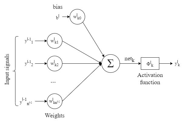
Figure 1: Scheme of the $k^{th}$ neuron in the $l^{th}$ layer of a MLP model. $\phi^{l}_{k}$ represent the activation function of the neuron, $b^{l}$ represent the bias of the $l^{th}$ layer, $y^{l-1}_{j}$ represent the output of the $j^{th}$ neuron in the previous layer and $w^{l}_{jk}$ represent the weight of the connection between the neuron and the $j^{th}$ neuron of the previous layer.

A fully-connected feed-forward MLP has one-way connections from the units of one layer to all neurons of the subsequent layer. Each time the output of one unit travels along one connection to another unit, it is multiplied by the weight of the connection. At each unit the inputs are summed and a constant, or bias, is added. Once all the input terms of each unit are summed, an activation function is applied to the result.

Figure 1 shows the scheme of a neuron in a MLP model and represent graphically the operations in Equation (1).

For each neuron, the output $y^{l}_{k}$ of the $k^{th}$ neuron in the $l^{th}$ layer can be calculated by:

$$y^{l}_{k}=\phi^{l}_{k}\left(z^{l}_{k}\right)=\phi^{l}_{k}\left(\sum_{j=1}^{n^{l-1}}w^{l}_{kj}\cdot y^{l-1}_{j}+w^{l}_{k0}\cdot b^{l}\right)$$ (1)

where $z^{l}_{k}$ refers to the weighted sum of the neuron inputs, $n^{l-1}$ refers to the number of neurons in the $(l-1)^{th}$ layer, $w^{l}_{kj}$ refers to the weight of the connection between the $j^{th}$ neuron in the $(l-1)^{th}$ layer and the $k^{th}$ neuron in the $l^{th}$ layer, $\phi^{l}_{k}$ refers to the activation function of the $k^{th}$ neuron in $l^{th}$ layer, $b^{l}$ refers to the bias in the $l^{th}$ layer and $\cdot$ refers to the scalar product operation. For the input layer thus holds $l=1$, $y^{1-1}_{j}=x_{j}$, $w^{1}_{kj}=1$ and $b^{1}=0$.

Figure 2 can be treated as a general MLP model. A MLP can have $L$ layers, and each layer $l$ ($1\leqslant l\leqslant L)$ has $n^{l}$ ($n^{l}\geqslant 1$) neurons. $n^{1}$ stands for the input layer and $n^{L}$ for the output layer. For each layer $l$ the input dimension is equal to the output dimension of layer $(l-1)$. For a neuron $i$ ($1\leqslant i\leqslant n^{l}$) in layer $l$, its input vector, weight vector and output are $\mathbf{yb}^{l-1}=\left(b^{l},y^{l-1}_{1},\cdots,y^{l-1}_{n^{l-1}}\right)$, $\mathbf{w}^{l}_{i}=\left(w^{l}_{i0},w^{l}_{i1},\cdots,w^{l}_{in^{l-1}}\right)^{\top}$ and $y^{l}_{i}=\phi^{l}_{i}\left(z^{l}_{i}\right)=\phi^{l}_{i}\left(\mathbf{yb}^{l-1}\cdot\mathbf{w}^{l}_{i}\right)$ respectively, where $\phi^{l}_{i}:\mathbb{R}\rightarrow\mathbb{R}$ refers to the neuron activation function and $\cdot$ refers to the matrix multiplication operator. For each layer $l$, its input vector is $\mathbf{yb}^{l-1}$, its weight matrix is $\mathbf{W}^{l}=\left[\mathbf{w}^{l}_{1}\cdots\mathbf{w}^{l}_{n^{l}}\right]$ and its output vector is $\mathbf{y}^{l}=\left(y^{l}_{i},\cdots,y^{l}_{n^{l}}\right)=\Phi^{l}\left(\mathbf{z}^{l}\right)=\Phi^{l}\left(\mathbf{yb}^{l-1}\cdot\mathbf{W}^{l}\right)$, where $\Phi^{l}:\mathbb{R}^{n^{l}}\rightarrow\mathbb{R}^{n^{l}}$ is a vector-valued function defined as $\Phi^{l}(\mathbf{z})=(\phi^{l}_{1}(z_{1}),\cdots,\phi^{l}_{n^{l}}(z_{n^{l}}))$.

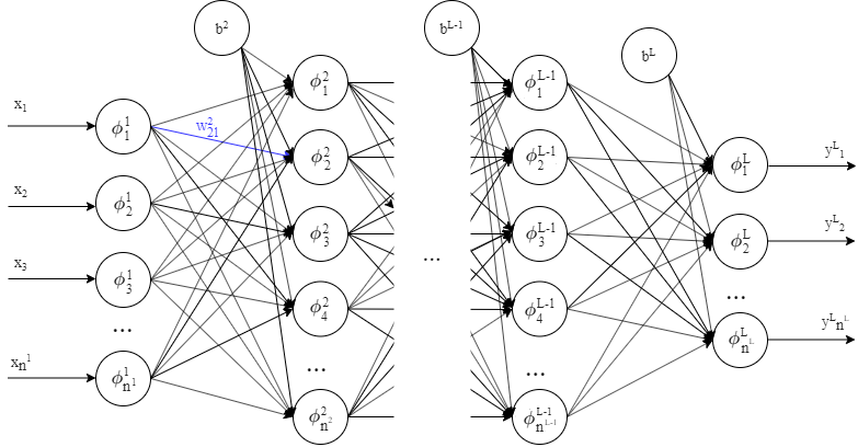
Figure 2: General MultiLayer Perceptron structure with $L$ layers. $\phi^{i}_{j}$ represent the activation function of the $j^{th}$ neuron in the $i^{th}$ layer, $b^{i}$ represent the bias of the $i^{th}$ layer, $x_{k}$ represent the input variables and $y_{k}$ represent the output variables.

Weights in the neural structure determine how the information flows from the input layer to the output layer. Identifying the optimal weights that minimize the prediction error of a dataset is called training the neural network. There are different algorithms to identify these weights, being the most used the backpropagation algorithm described in rumelhart_learning_1986. Explaining these training algorithms are out of the scope of this paper.

2.2 Partial derivatives

The sensitivity analysis performed by the NeuralSens package is based on the partial derivatives method. This method consists in calculating the derivative of the output with regard to the inputs of the neural network. These partial derivatives are called sensitivity, and are defined as:

$$s_{ik}\big{|}_{\mathbf{x}_{n}}=\frac{\partial y_{k}}{\partial x_{i}}\left(\mathbf{x}_{n}\right)$$ (2)

where $\mathbf{x}_{n}$ refers to the $n$ sample of the dataset used to perform the sensitivity analysis and $s_{ik}\big{|}_{\mathbf{x}_{n}}$ refers to the sensitivity of the output of the $k^{th}$ neuron in the output layer with regard to the input of the $i^{th}$ neuron in the input layer evaluated in $\mathbf{x}_{n}$. We calculate these sensitivities applying the chain rule to the partial derivatives of the inner layers (derivatives of Equation (1) for each neuron in the hidden layers). The partial derivatives of the inner layers are defined following the next equations:

• Derivative of $z^{l}_{k}$ (input of the $k^{th}$ neuron in the $l^{th}$ layer) with regard to $y^{l-1}_{i}$ (output of the $i^{th}$ neuron in the $(l-1)^{th}$ layer). This partial derivative corresponds to the weight of the connection between the $k^{th}$ neuron in the $l^{th}$ layer and the $i^{th}$ neuron in the $(l-1)^{th}$ layer:

  $$\frac{\partial z^{l}_{k}}{\partial y^{l-1}_{i}}=w^{l}_{ki}$$ (3)

• Derivative of $y^{l}_{k}$ (output of the the $k^{th}$ neuron in the $l^{th}$ layer) with regard to $z^{l}_{i}$ (input of the $i^{th}$ neuron in the $l^{th}$ layer):

  $$\left.\frac{\partial y^{l}_{k}}{\partial z^{l}_{i}}\right|_{z^{l}_{i}}=\frac{\partial\phi^{l}_{k}}{\partial z^{l}_{i}}\left(z^{l}_{i}\right)$$ (4)

  where $\frac{\partial\phi^{l}_{k}}{\partial z^{l}_{i}}$ refers to the partial derivative of the activation function of the $k^{th}$ neuron in the $l^{th}$ layer with regard to the input of the $k^{th}$ neuron in the $l^{th}$ layer evaluated for the input $z^{l}_{i}$ of the $i^{th}$ neuron in the $l^{th}$ layer.

Equations (3) and (4) have been implemented in the package in matrix form to reduce computational time following the next equations:

$$\frac{\partial\mathbf{z}^{l}_{[1\times n^{l}]}}{\partial\mathbf{y}^{l-1}_{[1\times n^{l-1}]}}=\left[{\begin{array}[]{cccc}\frac{\partial z^{l}_{1}}{\partial y^{l-1}_{1}}&\frac{\partial z^{l}_{2}}{\partial y^{l-1}_{1}}&\cdots&\frac{\partial z^{l}_{n^{l}}}{\partial y^{l-1}_{1}}\\ \frac{\partial z^{l}_{1}}{\partial y^{l-1}_{2}}&\frac{\partial z^{l}_{2}}{\partial y^{l-1}_{2}}&\cdots&\frac{\partial z^{l}_{n^{l}}}{\partial y^{l-1}_{2}}\\ \vdots&\vdots&\ddots&\vdots\\ \frac{\partial z^{l}_{1}}{\partial y^{l-1}_{n^{l-1}}}&\frac{\partial z^{l}_{2}}{\partial y^{l-1}_{n^{l-1}}}&\cdots&\frac{\partial z^{l}_{n^{l}}}{\partial y^{l-1}_{n^{l-1}}}\\ \end{array}}\right]=\left[{\begin{array}[]{cccc}w^{l}_{11}&w^{l}_{21}&\cdots&w^{l}_{n^{l}1}\\ w^{l}_{12}&w^{l}_{22}&\cdots&w^{l}_{n^{l}2}\\ \vdots&\vdots&\ddots&\vdots\\ w^{l}_{1n^{l-1}}&w^{l}_{2n^{l-1}}&\cdots&w^{l}_{n^{l}n^{l-1}}\\ \end{array}}\right]=\mathbf{W}^{*l}_{[n^{l-1}\times n^{l}]}$$ (5)

$$\mathbf{J}^{l}_{l_{[n^{l}\times n^{l}]}}=\frac{\partial{\mathbf{y}^{l}_{[1\times n^{l}]}}}{\partial{\mathbf{z}^{l}_{[1\times n^{l}]}}}=\left[{\begin{array}[]{cccc}\frac{\partial y^{l}_{1}}{\partial z^{l}_{1}}&\frac{\partial y^{l}_{2}}{\partial z^{l}_{1}}&\cdots&\frac{\partial y^{l}_{n^{l}}}{\partial z^{l}_{1}}\\ \frac{\partial y^{l}_{1}}{\partial z^{l}_{2}}&\frac{\partial y^{l}_{2}}{\partial z^{l}_{2}}&\cdots&\frac{\partial y^{l}_{n^{l}}}{\partial z^{l}_{2}}\\ \vdots&\vdots&\ddots&\vdots\\ \frac{\partial y^{l}_{1}}{\partial z^{l}_{n^{l}}}&\frac{\partial y^{l}_{2}}{\partial z^{l}_{n^{l}}}&\cdots&\frac{\partial y^{l}_{n^{l}}}{\partial z^{l}_{n^{l}}}\\ \end{array}}\right]=\left[{\begin{array}[]{cccc}\frac{\partial\phi^{l}_{1}}{\partial z^{l}_{1}}\left(z^{l}_{1}\right)&\frac{\partial\phi^{l}_{2}}{\partial z^{l}_{1}}\left(z^{l}_{1}\right)&\cdots&\frac{\partial\phi^{l}_{n^{l}}}{\partial z^{l}_{1}}\left(z^{l}_{1}\right)\\ \frac{\partial\phi^{l}_{1}}{\partial z^{l}_{2}}\left(z^{l}_{2}\right)&\frac{\partial\phi^{l}_{2}}{\partial z^{l}_{2}}\left(z^{l}_{2}\right)&\cdots&\frac{\partial\phi^{l}_{n^{l}}}{\partial z^{l}_{2}}\left(z^{l}_{2}\right)\\ \vdots&\vdots&\ddots&\vdots\\ \frac{\partial\phi^{l}_{1}}{\partial z^{l}_{n^{l}}}\left(z^{l}_{n^{l}}\right)&\frac{\partial\phi^{l}_{2}}{\partial z^{l}_{n^{l}}}\left(z^{l}_{n^{l}}\right)&\cdots&\frac{\partial\phi^{l}_{n^{l}}}{\partial z^{l}_{n^{l}}}\left(z^{l}_{n^{l}}\right)\\ \end{array}}\right]$$ (6)

where $\mathbf{W}^{*l}$ is the reduced weight matrix of the $l^{th}$ layer and $\mathbf{J}^{l}_{l}$ is the Jacobian matrix of the outputs in the $l^{th}$ layer with respect to the inputs in the $l^{th}$ layer.

Following the chain rule, the Jacobian matrix of the outputs in the $l^{th}$ layer with regard to the inputs in the $(l-j)^{th}$ layer can be calculated by:

$$\mathbf{J}^{l}_{l-j_{[n^{l}\times n^{j}]}}=\prod_{h=j}^{l-1}(\mathbf{J}^{h}_{h_{[n^{h}\times n^{h}]}}\cdot\mathbf{W}^{*(h+1)}_{[n^{h}\times n^{h+1}]})\cdot\mathbf{J}^{l}_{l_{[n^{l}\times n^{l}]}}$$ (7)

where $1\leqslant k\leqslant(l-1)$ and $2\leqslant l\leqslant L$. Using this equation with $l=L$ and $j=1$, the partial derivatives of the outputs with regard to the inputs of the MLP are obtained.

2.3 Sensitivity measures

Once the sensitivity has been obtained for each variable and observation, different measures can be calculated to analyze the results. The authors propose the following sensitivity measures to summarize the information obtained by evaluating the sensitivity of the outputs for all the input samples $X_{n}$ of the provided dataset:

• Mean sensitivity of the output of the $k^{th}$ neuron in the output layer with regard to the $i^{th}$ input variable:

  $$S_{ik}^{avg}=\frac{\sum_{j=1}^{N}s_{ik}\big{|}_{\mathbf{x}_{j}}}{N}$$ (8)

  where $N$ is the number of samples in the dataset.

• Sensitivity standard deviation of the output of the $k^{th}$ neuron in the output layer with regard to the $i^{th}$ input variable:

  $$S_{ik}^{sd}=\sigma\left(s_{ik}\big{|}_{\mathbf{x}_{j}}\right);j\in{1,...,N}$$ (9)

  where $N$ is the number of samples in the dataset and $\sigma$ refers to the standard deviation function.

• Mean squared sensitivity of the output of the $k^{th}$ neuron in the output layer with regard to the $i^{th}$ input variable (yeh_first_2010, zurada_sensitivity_1994):

  $$S_{ik}^{sq}=\sqrt{\frac{\sum_{j=1}^{N}\left(s_{ik}\big{|}_{\mathbf{x}_{j}}\right)^{2}}{N}}$$ (10)

  where $N$ is the number of samples in the dataset.

In case there are more than one output neuron, such as in a multi-class classification problem, these measures can be generalized to obtain sensitivity measures of the whole model as follows:

• Mean sensitivity with regard to the $i^{th}$ input variable:

  $$S_{i}^{avg}=\frac{\sum_{k=1}^{n^{l}}S_{ik}^{avg}}{n^{L}}$$ (11)

• Sensitivity standard deviation with regard to the $i^{th}$ input variable:

  $$S_{i}^{sd}=\sqrt{\frac{\sum_{k=1}^{n^{l}}\left(\left(S_{ik}^{sd}\right)^{2}+\left(S_{ik}^{avg}-S_{i}^{avg}\right)^{2}\right)}{n^{L}}}$$ (12)

• Mean squared sensitivity with regard to the $i^{th}$ input variable (yeh_first_2010):

  $$S_{i}^{sq}=\frac{\sum_{k=1}^{n^{l}}S_{ik}^{sq}}{n^{L}}$$ (13)

Methods in NeuralSens to calculate the sensitivities of a neural network and the proposed sensitivities measures were written for several R packages that can be used to create MLP neural networks: class ‘nn’ from neuralnet package (neuralnet), class ‘nnet’ from nnet package (nnet), class ‘mlp’ from RSNNS (RSNNS), classes ‘H2ORegressionModel’ and ‘H2OMultinomialModel’ from h2o package (h2o), ‘list’ from neural package (neural) and classnnetar from forecast package (forecast). The same methods are applied to neural network objects created with the train() function from the caret package (caret) only if these ‘train’ objects inherit from the available packages the “class” attribute. Methods have not been included in NeuralSens for other packages that can create MLP neural networks, although further developments of NeuralSens could include additional methods. An additional method for class ‘numeric’ is available to use with the basic information of the model (weights, structure and activation functions of the neurons). Examples on how to use this ‘numeric’ method can be found in appendix LABEL:app:ext_pack_func_impl.

3 Package structure

The functionalities of the package NeuralSens is based on the new R class ‘SensMLP’ defined inside the package itself. NeuralSens includes four main functions based on this class to perform the sensitivity analysis of a MLP model described in the previous section:

• SensAnalysisMLP(): S3 method to perform the sensitivity analysis using partial derivatives of the outputs with regard to the inputs of the MLP model. This function returns a ‘SensMLP’ object with the results of the sensitivity analysis.

• SensitivityPlots(): graphically represent the sensitivity measures of a ‘SensMLP’ object.

• SensFeaturePlot(): graphically represent the relation between the sensitivities of a ‘SensMLP’ object and the value of the input variables.

• SensTimePlot(): graphically represent the evolution among time of the sensitivities of a ‘SensMLP’ object.

Each of these functions are detailed in the rest of this section. The output of the last three functions are plots created with ggplot2 package functions (ggplot2).

3.1 The R class ‘SensMLP’

The NeuralSens package defines an S3 object called ‘SensMLP’ as a list with the following components:

• sens: ‘list’ of ‘data.frames’, one per neuron in the output layer, with the $S_{ik}^{avg}$, $S_{ik}^{sd}$ and $S_{ik}^{sq}$ sensitivity measures described in Section 2.3 (Equations (8), (9) and (10)). Each row of the data.frame contains the sensitivity measures with regard to a specific input.

• raw_sens: ‘list’ of ‘matrixes’, one per neuron in the output layer, with the sensitivities calculated following Equation (7) with $l=1$ and $L=L$. Each column of each ‘matrix’ contains the sensitivities of the output with regard to a specific input and each row contains the sensitivities with regard to all the inputs corresponding to the same row of the trData component.

• mlp_struct: ‘numeric’ ‘vector’ indicating the number of neurons in each layer of the MLP model.

• trData: typically a ‘data.frame’ which contains the dataset used to calculate the sensitivities.

• coefnames: ‘character’ ‘vector’ with the names of the input variables of the MLP model.

• output_name: ‘character’ ‘vector’ with the names of the output variables of the MLP model.

Functions described in Sections 3.3 (SensitivityPlots()), 3.4 (SensTimePlot()) and 3.5 (SensFeaturePlot()) can be accessed through the plot method of the ‘SensMLP’ object. print() and summary() methods are also available for obtaining information on the sensitivities and sensitivity measures of the ‘SensMLP’ object. Examples of these methods are presented in the remaining sections.

3.2 MLP Sensitivity Analysis

The SensAnalysisMLP() function calculates the partial derivatives of a MLP model. This function consists of an ‘S3’ method (s3_method) to extract the basic information of the model (weights, structure and activation functions) based on the model class attribute and to pass this information to the default method. This default method calculates the sensitivities of the model as described in Section 2, and creates a SensMLP object with the result of the sensitivity analysis. SensAnalysisMLP() function performs all operations using matrix calculus to reduce the computational time.

In the current version of NeuralSens (version 1.0.0), the accepted activation functions are shown in Table 1. To calculate the sensitivities, the function assumes that all the neurons in a defined layer has the same activation function.

Name	Function	Derivative
sigmoid	$f(z)=\frac{1}{1+e^{-z}}$	$\frac{\partial f}{\partial z}(z)=\frac{1}{1+e^{-z}}\cdot\left(1-\frac{1}{1+e^{-z}}\right)$
tanh	$f(z)=\tanh{(z)}$	$\frac{\partial f}{\partial z}(z)=1-\tanh{(z)}$
linear	$f(z)=z$	$f^{\prime}(z)=1$
ReLU	$f(z)=\begin{cases}\begin{aligned} 0&\quad\text{ when }z\leqslant 0\\ z&\quad\text{ when }z>0\\ \end{aligned}\end{cases}$	$\frac{\partial f}{\partial z}(z)=\begin{cases}\begin{aligned} 0&\quad\text{ when }z\leqslant 0\\ 1&\quad\text{ when }z>0\\ \end{aligned}\end{cases}$
arctan	$f(z)=\arctan{(z)}$	$\frac{\partial f}{\partial z}(z)=\frac{1}{1+e^{z}}$
softplus	$f(z)=\ln{\left(1+e^{z}\right)}$	$\frac{\partial f}{\partial z}(z)=\frac{1}{1+e^{-z}}$
softmax	$f_{i}(\mathbf{z})=\frac{e^{z_{i}}}{\sum\limits_{k}\left(e^{z_{k}}\right)}$	$\frac{\partial f_{i}}{\partial z_{j}}(\mathbf{z})=\begin{cases}\begin{aligned} f_{i}(\mathbf{z})\cdot(1-f_{j}(\mathbf{z}))&\quad\text{ when }i=j\\ -f_{j}(\mathbf{z})\cdot f_{i}(\mathbf{z})&\quad\text{ when }i\neq j\\ \end{aligned}\end{cases}$

Table 1: Accepted activation functions and their derivatives in SensAnalysisMLP(), where $z$ refers to the input value of the neuron as described in Equation (1) and $\mathbf{z}$ refers to the vector of input values of the neuron layer.

In order to show how SensAnalysisMLP() is used, we use a simulated dataset to train an MLP model of class ‘nn’ (RSNNS). The dataset consists of a ‘data.frame’ with 1500 rows of observations and four columns for three input variables (X1, X2, X3) and one output variable (Y). The input variables are random observations of a normal distribution with zero mean and standard deviation equal to 1. The output $Y$ is created following Equation (14) based on $X_{1}$ and $X_{2}$:

$$Y=(X_{1})^{2}-0.5\cdot X_{2}+0.1\cdot\varepsilon$$ (14)

where $\varepsilon$ is random noise generated using a normal distribution with zero mean and standard deviation equal to 1. $X_{3}$ is given to the model for training and a proper fitted model would find no relation between $X_{3}$ and $Y$.

?NeuralSens::simdata can be executed to obtain more information about the data. The library is loaded by executing the following code: R> library("NeuralSens") To test the functionality of the SensAnalysisMLP() function, mlp() function from RSNNS package trains a neural network model using the simdata dataset. R> library("RSNNS") R> set.seed(150) R> mod1 <- mlp(simdata[,c("X1","X2","X3")], simdata[,"Y"], maxit = 1000, + size = 10, linOut = TRUE) SensAnalysisMLP() is used to perform a sensitivity analysis to mod1 using the same dataset as in training: R> sens <- SensAnalysisMLP(mod1, trData = simdata, output_name = "Y", + plot = FALSE) sens is a ‘SensMLP’ object and methods of that class can be used to explore the sensitivity analysis: R> class(sens) [1] "SensMLP" R> summary(sens) Sensitivity analysis of 3-10-1 MLP network.

Sensitivity measures of each output: $YmeanstdmeanSensSQX1-0.0054069081.945242761.94476390X2-0.4855649310.067345040.49021056X3-0.0032006990.029710830.02987535\code{summary()}methodprintsthesensitivitymeasuresoftheoutputwithregardtotheinputsofthemodel.Thesemeasuresarecalculatedusingthesensitivitiesdisplayedwhenusingthe\code{print()}methoddescribedbelow.The\code{mean}column($S_ik^avg$)showsthemeaneffectoftheinputvariableontheoutput.The\code{std}column($S_ik^sd$)showsthevarianceoftheinputvariable^{\prime}seffectontheoutputalongtheinputspace.Thesecolumnsprovideinformationontherelationbetweeninputsandoutputvariables:\begin{itemize} \par\itemize@item@If both \code{mean} ($S_{ik}^{avg}$) and \code{std} ($S_{ik}^{sd}$) are near zero, it indicates that the output is not related to the input, because for all the training data the sensitivity of the output with regard to that input is approximately zero. \par\itemize@item@If \code{mean} ($S_{ik}^{avg}$) is different from zero and \code{std} ($S_{ik}^{sd}$) is near zero, it indicates that the output has a linear relationship with the input, because for all the training data the sensitivity of the output with regard tothat input is approximately constant. \par\itemize@item@If \code{std} ($S_{ik}^{sd}$) is different from zero, regardless of the value of \code{mean} ($S_{ik}^{avg}$), it indicates that the output has a non-linear relationship with the input, because the relation between the output and the input vary depending on the value of the input. \par\end{itemize}\par Settinganupperboundfor\code{std}tobeconsideredclosetozerosothattherelationshipbetweenoutputandinputcanbeconsideredaslinearisanon-trivialendeavor.Theauthorsareworkingonastatistictotestwhetherthefunctionalrelationshipbetweenaninputandanoutputvariablecanbeconsideredlinearand,ifsuccessful,itwillbeincludedinafutureversionofthepackage.\par\LTX@newpage Intheexample,the\code{mean}and\code{std}valuesshow:\begin{itemize} \par\itemize@item@$X_{1}$ has mean $\approx 0$ and standard deviation $\approx 2$. This means it has a non-constant, i.e., non-linear effect on the response variable. \par\itemize@item@$X_{2}$ has mean $\approx 0.5$ and standard deviation $\approx 0$. This means it has a constant, i.e., linear effect on the response variable. \par\itemize@item@$X_{3}$ has mean $\approx 0$ and standard deviation $\approx 0$. This means it has no effect on the response variable. \par\end{itemize}\par Aninputvariablemaybeconsideredsignificantiftheirsensitivities$s_ik|_x_j$aresignificantlydifferentfromzero,whethertheyarepositiveornegative.Inotherwords,avariableisconsideredtobesignificantwhenchangesintheinputvariableproducesignificantchangesintheoutputvariableofthemodel.\cite[cite]{\@@bibref{Authors Phrase1YearPhrase2}{white_statistical_2001}{\@@citephrase{(}}{\@@citephrase{)}}}concludethatthestatistic$(S_ik^sq)^2 = ∑j = 1N(sik|xj)2N$isavalidindicatortoidentifyifavariableisirrelevant.Moreover,$S_ik^sq$isameasureofthechangesintheoutputduetolocalchangesintheinput.Thus,$S_ik^sq$canbedefinedasameasureoftheimportanceoftheinputvariablesfromaperturbationanalysispointofview,inthesensethatsmallchangesinthatinputwillproducelargerchangesintheoutput.\par`\code{SensMLP}^{\prime}classhasalsoa\code{print()}methodtoshowthesensitivitiesoftheoutputwithregardtotheinputsevaluatedineachoftherowsofthe\code{trData}componentofthe\code{sens}object.Asecondargument\code{n}maybeusedtospecifyhowmanyrowstodisplay(bydefault\code{n=5}).\CodeChunk\CodeInput R>print(sens,n=2)\CodeOutput Sensitivityanalysisof3-10-1MLPnetwork.\par 2000samples\par Sensitivitiesofeachoutput(only2firstsamples):$YX1X2X3[1,]2.08642384-0.4462707-0.044063158[2,]-0.34976334-0.35473810.014188363$

3.3 Visualizing Neural Network Sensitivity Measures

Sensitivity measures of the output variables are useful for quantitative analysis. However, it can be difficult to compare sensitivity metrics when a large number of input variables are used. In order to visualize information on the calculated sensitivities, the authors propose the following plots:

1. Label plot representing the relationship between $S_{ik}^{avg}$ (x-axis) and $S_{k}^{std}$ (y-axis).

2. Bar plot that shows $S_{k}^{sq}$ for each input variable.

3. Density plot that shows the distribution of output sensitivities with regard to each input (muoz_variable_1998):

   • The narrow distribution of sensitivity values for X2 (corresponding to a constant sensitivity) indicates a linear relationship between this input and the output of the neural net.

   • The wide distribution of sensitivity values for X1 (corresponding to a variable sensitivity) indicates a non-linear relationship between this input and the output.

   When the height of at least one of the distributions is greater than 10 times the height of the smallest distribution, then an extra plot is created using the facet_zoom() function of the ggforce package (ggforce). These plots provides a better representation of the sensitivity distributions.

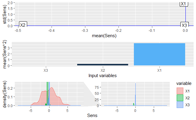
Figure 3: Example from the SensitivityPlots() function showing plots specified in Section 3.3. First plot shows the relation between the mean and standard deviation of the sensitivities, the second plot shows the square of the sensitivities and the third and fourth plots show the distribution of the sensitivities.

These plots can be obtained using the SensitivityPlots() function and a ‘SensMLP’ object calculated using SensAnalysisMLP(). To obtain the plots of Figure 3: R> SensitivityPlots(sens) Or they can be generated using the plot() method of the ‘SensMLP’ object: R> plot(sens) In this case, the first plot of Figure 3 shows that Y has a negative linear relationship with X2 ($std\approx 0$ and $mean<0$), no relationship with X3 ($std\approx 0$ and $mean\approx 0$) and a non-linear relationship with X1 ($std$ different from $0$). The second plot shows that X3 barely affects the response variable, being X1 and X2 the inputs with most effect on the output.

3.4 Visualizing Neural Network Sensitivity over time

A common application of neural networks is time series forecasting. Analyzing how sensitivities evolve over time can provide a better understanding of the effect of explanatory variables on the output variables.

SensTimePlot() returns a sequence plot of the raw sensitivities calculated by the function SensAnalysisMLP(). The x-axis is related to a numeric or Posixct/Posixlt variable containing the time information of each sample. The y-axis is related to the sensitivities of the output with regard to each input.

In order to show how this function can be used, the DAILY_DEMAND_TR dataset is used to create a model of class ‘train’ from caret package (caret). This dataset is similar to the elecdaily dataset from fpp2 R package (fpp2). However, DAILY_DEMAND_TR contains almost five years of daily data (elecdaily only one year), which makes it more suitable for training a neural network. It is composed of the following variables:

• DATE: date of the sample, one per day from July, 2nd 2007 to November, 30th 2012.

• TEMP: mean daily temperature in ºC in Madrid, Spain.

• WD: working day, continuous parameter which represents the effect on the daily consumption of electricity as a percentage of the expected electricity demand of that day with regard to the demand of the reference day of the same week moral-carcedo_modelling_2005. In this case, Wednesday is the reference day (WD${}_{Wed}\approx 1$).

• DEM: total daily electricity demand in GWh for Madrid, Spain.

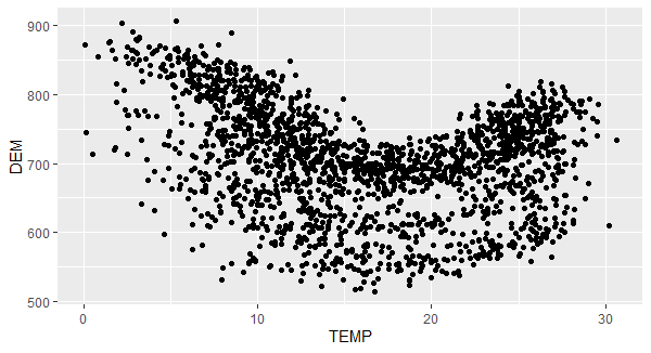
Figure 4: Relation between the output variable, DEM, and the input TEMP of DAILY_DEMAND_TR database.

The following code creates the plot in Figure 4: R> library("ggplot2") R> ggplot(DAILY_DEMAND_TR) + geom_point(aes(x = TEMP, y = DEM)) Figure 4 shows the relationship between the electricity demand and the temperature. A non-linear effect can be observed, where the demand increases for low temperatures (due to heating systems) and for high temperatures (due to air conditioners).

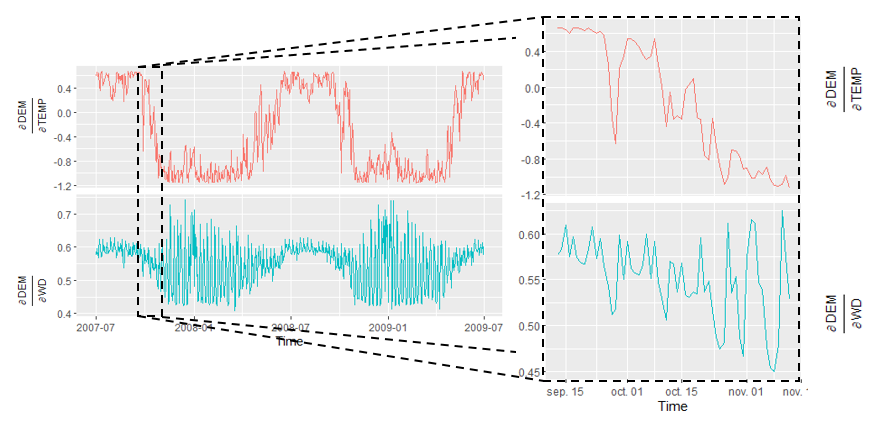
Figure 5: Example from the SensTimePlot() function, showing how the sensitivities for each of the inputs evolve over time.

The following code scales the data, create a train neural network model and apply the SensTimePlot() function to two years of the data: R> DAILY_DEMAND_TR[,4] <- DAILY_DEMAND_TR[,4]/10 R> DAILY_DEMAND_TR[,2] <- DAILY_DEMAND_TR[,2]/100 R> library("caret") R> set.seed(150) R> mod2 <- train(form = DEM TEMP + WD, data = DAILY_DEMAND_TR, + method = "nnet", linout = TRUE, maxit = 250, metric = "RMSE", + tuneGrid = data.frame(size = 5, decay = 0.1), + preProcess = c("center","scale"), trControl = trainControl()) R> SensTimePlot(mod2, DAILY_DEMAND_TR[1:(365*2),], output_name = "DEM", + date.var = DAILY_DEMAND_TR[1:(365*2),1], facet = TRUE) Figure 5 shows that the temperature variable has a seasonal effect on the response variable. In summer, the temperature is higher and cooling systems demand more electricity, therefore the demand is directly proportional to the temperature. In winter, the temperature is lower and heating systems demand more electricity, hence the demand is inversely proportional to the temperature. The sensitivity of the output with regard to WD has also a seasonal effect, with higher variance in winter than in summer and greater sensitivity in weekends. Figure 5 can also be generated using the plot() method of a ‘SensMLP’ object: R> sens2 <- SensAnalysisMLP(mod2, trData = DAILY_DEMAND_TR[1:(365*2),], + output_name = "DEM", plot = FALSE) R> plot(sens2, plotType = "time", facet = TRUE, + date.var = DAILY_DEMAND_TR[1:(365*2),1])

3.5 Visualizing the Neural Network Sensitivity relation as a function of the input values

Sometimes it is useful to know how the value of the input variables affects the sensitivity of the response variables. The SensFeaturePlot() function produces a violin plot to show the probability density of the output sensitivities with regard to each input. It also plots a jitter strip chart for each input, where the width of the jitter is controlled by the density distribution of the data (ggforce). The color of the points is proportional to the value of each input variable, which display whether the relation of the output with the input is relatively constant within a range of input values.

The following code produce the plot of Figure 6: R> SensFeaturePlot(mod2, fdata = DAILY_DEMAND_TR[1:(365*2),])

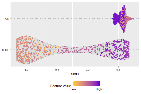
Figure 6: Example from the SensFeaturePlot() function, showing the relationship of the sensitivities with the value of the inputs.

It can also be generated using the plot() method of a ‘SensMLP’ object: R> plot(sens2, plotType = "features") In accordance with the information extracted from Figure 5, Figure 6 shows that the sensitivity of the output with regard to the temperature is negative when the temperature is low and positive when the temperature is high. It also shows that the sensitivity of the output with regard to WD is higher in the weekends (lower values of WD).

3.6 Extending package functionalities to other MLP models

The current version of NeuralSens package (version 1.0.0), includes methods of SensAnalysisMLP() function for ‘nn’ (neuralnet), ‘nnet’ (nnet), ‘H2ORegressionModel’ and ‘H2OMultinomialModel’ (h2o), ‘mlp’ (RSNNS), ‘list’ (neural), ‘nnetar’ (forecast) and ‘train’ (caret) (only if the object inherits the class attribute from another of the available packages). Additionally, a ‘numeric’ method is available to perform sensitivity analysis of a new neural network model using only the weights of the model, its neural structure, and the activation function of the layers and their derivatives. The first information that must be extracted from the model are the weights of the connections between layers. These weights must be passed to the first argument of the SensAnalysisMLP() function as a ‘numeric’ ‘vector’, concatenating the weights of the layers in order from the first hidden layer ($l=2$) to the output layer ($l=L$). The bias weight should be added to the vector before the weights of the same layer, following the equation below:

$$wts=[b^{2},w^{2}_{11},w^{2}_{21},...,w^{2}_{n^{2}n^{1}},b^{3},w^{3}_{11},...,b^{L},w^{L}_{11},...,w^{L}_{n^{L}n^{L-1}}]$$ (15)

If the model has no bias, the bias weights must be set to 0 ($b^{l}=0$).

The second information is the neural structure of the model. The structure of the model must be passed to the mlpstr argument as a ‘numeric’ ‘vector’ equal in length to the number of layers in the network. Each number specifies the number of neurons in each layer, starting with the input layer and ending with the output layer:

The last information that must be provided are the activation functions of each layer and their derivatives. If the activation function of a layer is one of those provided by the package (shown in Table 1), the function can be specified using its name. If the activation function is not one of those provided in the package, it should be passed as a function. The same applies to the derivative of the activation function. The activation function $\Phi^{l}(\mathbf{z}^{l})$ of a layer $l$ and its derivative $\frac{\partial(\Phi^{l}(\mathbf{z}^{l}))}{\partial(\mathbf{z}^{l})}$ must meet the following conditions:

• $\Phi^{l}(\mathbf{z}^{l})$ must return a ‘vector’ with the same length as $\mathbf{z}^{l}$. The activation function of each neuron may be different, as long as this condition is met:

  $$\Phi^{l}(\mathbf{z}^{l}) =\begin{bmatrix}\phi^{l}_{1}(z^{l}_{1})\\ \phi^{l}_{2}(z^{l}_{2})\\ \vdots\\ \phi^{l}_{n^{l}}(z^{l}_{n^{l}})\end{bmatrix}$$ (16)

• $\frac{\partial(\Phi^{l}(\mathbf{z}^{l}))}{\partial(\mathbf{z}^{l})}$ must return a square ‘matrix’ with the derivative of $\Phi^{l}(\mathbf{z}^{l})$ with regard to each component of $\mathbf{z}^{l}$:

  $$\frac{\partial(\Phi^{l}(\mathbf{z}^{l}))}{\partial(\mathbf{z}^{l})}=\left[{\begin{array}[]{cccc}\frac{\partial\phi^{l}_{1}}{\partial z^{l}_{1}}\left(z^{l}_{1}\right)&\frac{\partial\phi^{l}_{2}}{\partial z^{l}_{1}}\left(z^{l}_{1}\right)&\cdots&\frac{\partial\phi^{l}_{n^{l}}}{\partial z^{l}_{1}}\left(z^{l}_{1}\right)\\ \frac{\partial\phi^{l}_{1}}{\partial z^{l}_{2}}\left(z^{l}_{2}\right)&\frac{\partial\phi^{l}_{2}}{\partial z^{l}_{2}}\left(z^{l}_{2}\right)&\cdots&\frac{\partial\phi^{l}_{n^{l}}}{\partial z^{l}_{2}}\left(z^{l}_{2}\right)\\ \vdots&\vdots&\ddots&\vdots\\ \frac{\partial\phi^{l}_{1}}{\partial z^{l}_{n^{l}}}\left(z^{l}_{n^{l}}\right)&\frac{\partial\phi^{l}_{2}}{\partial z^{l}_{n^{l}}}\left(z^{l}_{n^{l}}\right)&\cdots&\frac{\partial\phi^{l}_{n^{l}}}{\partial z^{l}_{n^{l}}}\left(z^{l}_{n^{l}}\right)\\ \end{array}}\right]$$ (17)

Examples of how to use the SensAnalysisMLP() function with new packages can be found in Appendix LABEL:app:ext_pack_func_impl.

3.7 Effect of network structure and training conditions

An important advantage of sensitivity analysis based on partial derivatives is the robustness of the analysis results regardless of the model’s neural structure. Other methods such as Olden rely heavily on the neural structure and the initial starting weights. A similar analysis to the one performed on olden() in beck_neuralnettools_2018 has been performed on the SensAnalysisMLP() function. To observe the effect of the neural structure on the sensitivity metrics, these metrics have been calculated for models with 1, 10 and 20 neurons in the hidden layer. For each neuron level, 50 models with different random initial weights are trained. If the neural structure and the initial starting weights have no effect on the sensitivity metrics, these metrics should be the same for all the models. simdata dataset is used to train the models.

Figure 7 shows the mean value of the sensitivity metrics from the 50 models for each neural structure. It also shows the minimum and maximum value of the metric to display the effect of the neural structure and the initial weights values. An important conclusion that can be derived from Figure 7 is that with enough neurons in the hidden layer, i.e., if the model can predict the output with enough precision; variance of sensitivity metrics is negligible compared to the value of the metric.

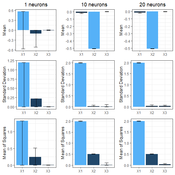
Figure 7: Robustness analysis of sensitivity metrics for three neural network models with different number of neurons in the hidden layer. Fifty different models for each neuron level are trained with random initial weights. geom_bar shows the mean value of the sensitivity metrics and geom_errorbar shows the minimum and maximum value of the sensitivity metrics.

4 Further examples and comparison with other methods

This section contains several examples in which the functions of the NeuralSens package are compared with similar functions from other R packages. Section 4.1 trains an MLP for classification to compare SensAnalysisMLP() with olden(), garson() (beck_neuralnettools_2018) and plot_explanations() (lin_pedersen_understanding_2019). Section LABEL:subsec:mlp_reg trains an MLP for regression to compare SensAnalysisMLP() and SensFeaturePlot() with lekprofile() (beck_neuralnettools_2018) and partial() (pdp).

Topics such as data pre-processing or network architecture should be considered before model development. Discussions about these ideas have been already held (cannas_data_2006, amasyali_review_2017, maier_neural_1999, lek_application_1996) and are beyond the scope of this paper.

4.1 Multilayer perceptron for classification

In this example a multilayer perceptron is trained using the well-known iris dataset included in R. Figure 8 shows two scatterplots comparing the petal-related and sepal-related variables of the flowers in the dataset. It can be seen that setosa species have a smaller petal size than the other two species and a shorter sepal. It also shows that virginica and versicolor species have a similar sepal size, but the latter has a slightly smaller petal size.

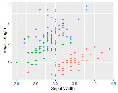
(a) Sepal-related variables

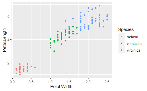
(b) Petal-related variables

Figure 8: (8(a)) geom_point plot representing the variables Sepal.Length and Sepal.Width, (8(b)) geom_point plot representing the variables Petal.Length and Petal.Width

The train() function from the caret package creates a new neural network model to predict the species of each flowers based on petal and sepal dimensions. R> set.seed(150) R> mod3 <- caret::train(Species ., data = iris, preProcess = c("center", + "scale"), method = "nnet", linout = TRUE, trControl = trainControl(), + tuneGrid = data.frame(size = 5, decay = 0.1), metric = "Accuracy") SensAnalysisMLP() function calculates the sensitivities of the model, providing information of the relationships between each output class and each input variable. R> sens4 <- SensAnalysisMLP(mod3) R> summary(sens4) Sensitivity analysis of 4-5-3 MLP network.

Sensitivity measures of each output: $setosameanstdmeanSensSQSepal.Length-0.013460270.026982450.03007287Sepal.Width0.031166690.050555890.05924712Petal.Length-0.071339250.101721960.12396638Petal.Width-0.068463950.096540300.11808983\par$versicolor mean std meanSensSQ Sepal.Length 0.035833076 0.02252307 0.04228375 Sepal.Width -0.002101449 0.03925762 0.03918294 Petal.Length -0.099221391 0.17568963 0.20126091 Petal.Width -0.093949654 0.16300239 0.18766775

$virginicameanstdmeanSensSQSepal.Length-\mathrm{0.018031390.027423340.03274380}Sepal.Width-\mathrm{0.041998560.056631250.07035338}Petal.Length\mathrm{0.205435150.284135480.34985476}Petal.Width\mathrm{0.197310970.272367350.33559057}\text{Figure 9Figure 99Figure 9(a)9(a)9(a)(a)Model 3, codeSensitivityPlots()(a)Model 3, codeSensitivityPlots()(b)9(b)9(b)(b)Model 3, codegarson()(b)Model 3, codegarson()(c)9(c)9(c)(c)Model 3, codeolden()(c)Model 3, codeolden()9(9(a))}$