Analytical Equations based Prediction Approach for PM2.5 using Artificial Neural Network

Abstract

Particulate matter pollution is one of the deadliest types of air pollution worldwide due to its significant impacts on the global environment and human health. Particulate Matter (PM2.5) is one of the important particulate pollutants to measure the Air Quality Index (AQI). The conventional instruments used by the air quality monitoring stations to monitor PM2.5 are costly, bulkier, time-consuming, and power-hungry. Furthermore, due to limited data availability and non-scalability, these stations cannot provide high spatial and temporal resolution in real-time. To overcome the disadvantages of existing methodology this article presents analytical equations based prediction approach for PM2.5 using an Artificial Neural Network (ANN). Since the derived analytical equations for the prediction can be computed using a Wireless Sensor Node (WSN) or low-cost processing tool, it demonstrates the usefulness of the proposed approach. Moreover, the study related to correlation among the PM2.5 and other pollutants is performed to select the appropriate predictors. The large authenticate data set of Central Pollution Control Board (CPCB) online station, India is used for the proposed approach. The RMSE and coefficient of determination (R²) obtained for the proposed prediction approach using eight predictors are 1.7973 µg/m³ and 0.9986 respectively. While the proposed approach results show RMSE of 7.5372 µg/m³ and R² of 0.9708 using three predictors. Therefore, the results demonstrate that the proposed approach is one of the promising approaches for monitoring PM2.5 without power-hungry gas sensors and bulkier analyzers.

1 Introduction

Meteorological parameters such as temperature, humidity, light, air velocity and gaseous pollutants such as Carbon Dioxide (CO₂), Carbon Monoxide (CO), Nitrogen Dioxide (NO₂), Sulphur Dioxide (SO₂), Volatile Organic Compounds (VOCs), Suspended Particulate Matter (SPM), and Ozone (O₃) express the environment quality. The main sources of these pollutants are industrial, residential, transportation, trading, agricultural, and natural activities such as combustion of fuels, wood fire, and forest fire, etc. airsourcecpcb ; airsourceepa . In India, the Central Pollution Control Board (CPCB) is responsible for providing the ambient Air Quality Index (AQI) through the National Air Quality Monitoring Programme (NAMP). The NAMP NAMP network consists of approximately 683 monitoring stations deployed across 300 cities/towns in 29 states and 6 union territories of the country. The objectives of NAMP are to determine the status and trends of ambient air quality and check the prescribed upper and lower limits of the air quality and take corrective measures for the AQI AQIreport . The AQI transforms the air quality data into a number, nomenclature, color, and a category; Good, Satisfactory, Moderately Polluted, Poor, Very Poor and Severe based on their health impacts. The overall AQI AQI is calculated from a minimum three pollutants out of which one should be the Particulate Matter (PM2.5) which can potentially cause serious health problems.

PM2.5 poses a major concern for human health as due to its small size ($<$ 2.5µm) they can directly enter into the lungs WHOreport . PM2.5 comes either from primary sources or from secondary sources. The primary sources can be vehicles, power plants, wood burning, industrial processes, forest or grass fires, and agricultural burning processes. The secondary sources are precursor emissions such as Sulfur dioxide (SO₂), Oxides, Volatile Organic Compounds (VOCs), and Ammonia (NH₃) WHOreport ; hodan . Though different methods and instruments for monitoring PM2.5 exist amaral2015overview , only a few are used for real-time measurement and monitoring. These instruments for PM2.5 often lack portability and exhibit a slower response time budde2014distributed . Furthermore, the standard procedure to collect samples through samplers and analyzing them offline in specialized laboratories is challenging for real-time monitoring and corrective actions NAAQsample ; pm2.52 . This is because analyzed data is a delayed response of the current data. Hence real-time monitoring of PM2.5 can be useful. In this work, we propose a method to address the issue of the delayed response of data. We propose the PM2.5 prediction model based on analytical equations, which can be ported to a standard Wireless Sensor Node (WSN). We envisage that such a method not only provides benefits for real-time monitoring but also enables an existing WSN to extend its capabilities from monitoring to analyzing.

2 Related Work

The classification of both direct and indirect measurements for outdoor environmental monitoring is shown in Fig. 1. In direct methods, dedicated instruments such as analyzers NAAQsample , aethalometer Vilcassim2014 , samplers gehrig2003characterising ; northcross2010estimating ; querol2001monitoring ,

and in certain cases Wireless Sensor Nodes (WSNs) hall2012portable ; mansour2014wireless ; kasar2013wsn ; liu2011developed are used. Aethalometer and analyzers provide the pollutants’ values directly but lack portability and are often expensive. In air pollution monitoring using samplers, offline analysis is done in specialized laboratories. Whereas in wireless sensor nodes, the measurement of pollutants is done using on-board gas sensors and is often a cost-effective solution compared to other monitoring methods yi2015survey . An example of such a system deployed in a New York subway is discussed in Vilcassim2014 .

for tree= align=center, parent anchor=south, child anchor=north, font=, edge=thick, -Stealth[], l sep+=10pt, edge path= [draw, edge] (!u.parent anchor) – +(0,-10pt) -— (.child anchor)edge label; , [Outdoor Monitoring [Direct Methods [Analyzer
NAAQsample ] [Aethalometer
Vilcassim2014 ] [Sampler
gehrig2003characterising ; northcross2010estimating ; querol2001monitoring ] [WSN
hall2012portable ; mansour2014wireless ; kasar2013wsn ; liu2011developed ] ] [Indirect Methods [Prediction model based on
past data of predictand,
meteorological parameters
and other pollutants
Ordieres2005 ; Jef2005 ; emp6 ; nn6 ; lu2006prediction ; Sousa2007 ; gardner1999neural ; grivas2006artificial ; ann6 ; ann7 ; ann5 ; nc8 ; nc28 ; A2006 ; diaz2008hybrid ; ann25 ; clusternn ; hybrid5 ; hybrid7 ; hybrid6 ; regularization ; cgmmodel7 ; deeplearning ; deeplearning2 ; deeplearning6 ] [Prediction model based on
correlated meteorological parameters
and pollutants
corr27 ; corr7 ; everyaware [Proposed Method
(Prediction model
based on
correlated pollutants,
as analytical equations)] ] ] ] ]

Figure 1: Direct and Indirect Methods of Prediction of Pollutants for Outdoor Monitoring

The indirect measurements Ordieres2005 ; Jef2005 ; emp6 ; nn6 ; lu2006prediction ; Sousa2007 ; gardner1999neural ; grivas2006artificial ; ann6 ; ann7 ; ann5 ; nc8 ; nc28 ; A2006 ; diaz2008hybrid ; ann25 ; clusternn ; hybrid5 ; hybrid6 ; regularization ; cgmmodel7 ; deeplearning ; deeplearning2 ; deeplearning6 used prediction approach based on the past data of the predictand, pollutants and/or meteorological parameters. These pollutants and meteorological parameters are correlated with the predictand hybrid7 ; corr27 ; corr7 ; everyaware . The PM2.5 (predictand) can be forecasted based on the data of pollutants and meteorological parameters which are correlated with PM2.5. The performance comparison of different prediction techniques of greenhouse gas is discussed in predictionmethodsreview . In Ordieres2005 , a comparison of different topologies of a neural network is presented for a prediction model of PM2.5. A neural network-based prediction model for PM10 using previous days data for PM10, cloud cover, boundary layer height, wind direction and day of the week is discussed in Jef2005 . For the prediction of PM2.5 and O₃, the empirical non-linear regression model was designed emp6 using meteorological parameters and past PM2.5 data. In nn6 feed-forward neural network is used for prediction of PM2.5 based on past values of PM10, PM2.5 and some observed and forecasted meteorological parameters. In lu2006prediction ; Sousa2007 , prediction based on ANN using past data of O₃ is discussed. A Multilayer Perceptron (MLP) neural network-based prediction model gardner1999neural for NO and NO₂ pollutants is developed using past data of pollutants. In grivas2006artificial prediction model show MLP neural network has better performance than Multiple Linear Regression (MLR) model. Results in ann6 demonstrates the better performance of ANN compared to MLR for prediction of PM2.5 in the agricultural park. Comparison results of MLR and ANN in ann7 , for prediction of PM2.5 represents the better performance of ANN. Feed Forward Neural Network (FFNN) with Rolling Mechanism (RM) and Accumulated Generating Operation (AGO) of Gray model (RM-GM-FFNN) was developed ann5 for prediction of PM2.5 and PM10 using past data of PM2.5 and PM10 in addition to meteorological data. Prediction of PM2.5 based on the Back Propagation (BP) neural network was explored nc8 using satellite-based Aerosol Optical Depth (AOD), meteorological data and past PM2.5 data. The optimized version of the BP network using a genetic algorithm is proposed in nc28 .

Few researchers have also explored the hybrid model approach for prediction. A hybrid approach based on the autoregressive and nonlinear model for prediction of NO₂ is proposed in A2006 . A hybrid approach based on Autoregressive Integrated Moving Average Model (ARIMA) and ANN is discussed in diaz2008hybrid . The Comprehensive Forecasting Model (CFM) was developed based on ARIMA, ANN and Exponential Smoothing Method (ESM) ann25 . Another cluster-based hybrid approach using Neural Network Autoregression (NNAR) and the ARIMA model is discussed in clusternn for prediction of PM2.5 using past data of PM2.5. A hybrid-generalized autoregressive conditional heteroskedasticity based prediction approach proposed in hybrid7 for prediction of PM2.5. In hybrid5 hybrid model was built for PM2.5 by applying the trajectory-based geographic model and wavelet transformation into the MLP type of neural network. In which meteorological forecasts and pollutants were used as predictors. Comparison of a hybrid model consisting of an Ensemble Empirical Mode Decomposition and General Regression Neural Network (EEMD-GRNN), Adaptive Neuro-Fuzzy Inference System (ANFIS), Principal Component Regression (PCR), and MLR is discussed in hybrid6 with best results obtained for EEMD-GRNN model. In regularization multi-task learning framework is used for the prediction of air pollutants which reduces model parameters with improved performance. Convolutional generalization model implemented cgmmodel7 for prediction of PM2.5 using meteorological data shows MSE of 15.0 µg/m³. A deep learning-based prediction approach is also implemented for prediction using current and/or previous air pollutants and meteorological data deeplearning ; deeplearning2 ; deeplearning6 .

The research work in corr27 focused on Cuckoo Search-Least Squares Support Vector Machine (CS-LSSVM) based prediction approach for PM2.5 using correlation and principal component analysis. Previous data of PM2.5 was used as one of the predictors in addition to correlated parameters. The correlation analysis of PM2.5 to other meteorological parameters and pollutants using multivariate statistical analysis method and ANN was implemented in corr7 and prediction results show RMSE of 24.06 µg/m³ for ANN-based model. Performance comparison of machine learning approaches such as Random Forests (RF), Support Vector Machines (SVMs) and ANN is presented in everyaware . Furthermore, a calibration model is developed using ANN for black carbon in which meteorological parameter and other correlated pollutants are used as predictors. The lower RMSE and R² closeness to 1, also showed the effectiveness of the ANN.

However, the previously developed prediction model based on past data of predictand does not eliminate the need for dedicated instruments and in almost all cases the proprietary tools are used to measure the predictand. This presents an opportunity for developing a prediction model in the form of analytical equations based on the correlation. The ANN is adopted in our work, due to its superior performance discussed in lu2006prediction ; Sousa2007 ; gardner1999neural ; grivas2006artificial ; ann6 ; ann7 ; everyaware . Primary results related to the comparison of SVM and ANN are discussed in the results section and demonstrate the effectiveness of our proposed method.

The contribution of the work is as follows:

1. The study related to correlation of the pollutants with PM2.5 and additionally the correlation among the pollutants is performed for deciding the predictors.

2. Analytical equations are proposed for prediction of PM2.5 using ANN.

3. Recalibration of the derived prediction model in terms of coefficients and number of predictors is done to evaluate its performance.

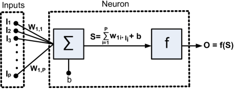
Figure 2: ANN Model of a Neuron

3 Introduction to ANN Model

The proposed prediction model to obtain PM2.5 is based on supervised machine learning. It consists of interconnected computing elements known as neurons with inputs and outputs. As shown in Fig. 2, the model of a neuron has $P$ inputs each with weight $W$. The sum ($S$) of weighted inputs and bias ($b$) is fed to the transfer function block ($f$). The output of each neuron is obtained by subsequently applying the transfer function to the sum of weighted inputs and bias.

The proposed PM2.5 prediction model using the ANN is derived using the following steps.

1. Collection of large input data (observations) set for different pollutants.

2. Preprocessing of the input data set to remove outliers.

3. Finding correlation of PM2.5 with other pollutants using preprocessed input data set.

4. Based on the correlation results selection of input pollutants (predictors) for developing the prediction model of PM2.5.

5. Selection of ANN topology for developing the prediction model.

6. Division of predictors data set into two sets, SET1: 90% of data set or developing model (training, validation, and testing), SET2: 10% of data set as unseen data set for further testing.

7. Developing 100 different ANNs with randomly initialized weights and biases using SET1.

8. Testing of 100 different ANNs using SET2.

9. Based on performance indices selection of best ANN for the prediction model.

10. Deriving analytical equation for prediction using selected ANN.

11. Prediction of PM2.5 using derived analytical prediction equation.

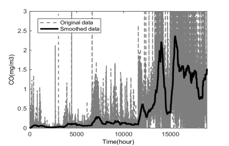
(a) CO Data

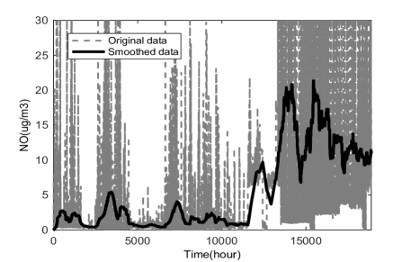
(b) NO Data

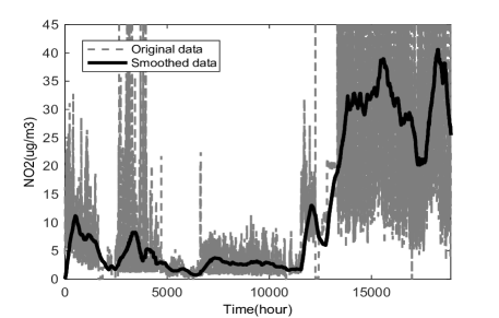
(c) NO₂ Data

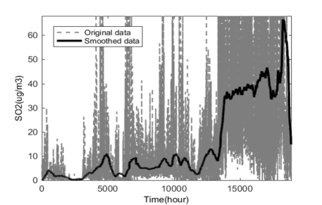
(d) SO₂ Data

Figure 3: Original and Smoothed Data of CO, NO and NO₂ and SO₂

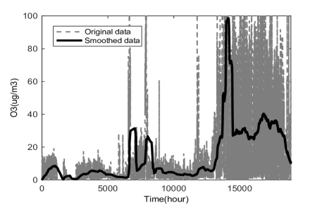
(a) O₃ Data

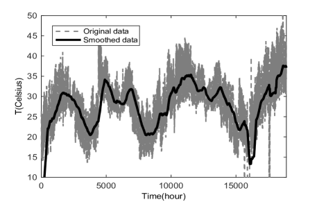
(b) Temperature Data

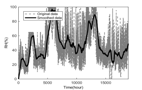
(c) Humidity Data

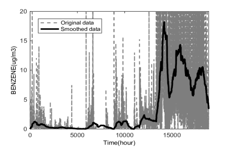
(d) Benzene Data

Figure 4: Original and Smoothed Data of O₃, Temperature, Humidity and Benzene

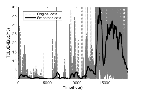
(e) Toluene Data

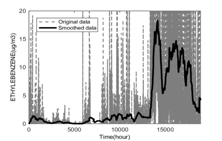
(f) Ethyl Benzene Data

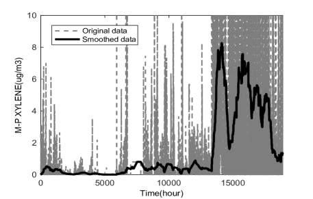
(g) M-P Xylene Data

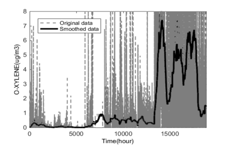
(h) O-Xylene Data

Figure 5: Original and Smoothed Data of Toluene, Ethyl Benzene, M-P Xylene and O-Xylene

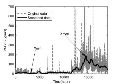
Figure 6: PM2.5 Data

4 Observed Data and Correlation

To select the inputs for the PM2.5 prediction model, it is necessary to obtain the correlation between PM2.5 and pollutants besides the correlation among the pollutants. In the proposed study, Step I is the data collection phase: In this phase, 13 different parameters (pollutants and meteorological parameters) were collected from a CPCB online station, India (N 23^∘ 0’ 16.6287, E 72^∘ 35’ 48.7816). The data is collected for 41 months, where, the samples of data are taken every hour. Thirteen different parameters monitored from this online station includes pollutants; CO, NO, NO₂, SO₂, O₃, VOC (Benzene, Toluene, Ethyl Benzene, M+P Xylene, O-Xylene), PM2.5 and meteorological parameters; temperature and humidity. Dataset obtained from CPCB online station for all 13 parameters was containing a total of 29,928 observations. Due to maintenance, all the parameters data were not available simultaneously for 29,928 observations. After removing maintenance data for each of the parameters, 18,880 observations data set was available simultaneously for all 13 parameters. These 18,880 observations data set was smoothed out to remove the outliers [Step II] and is treated as the golden standard data. The smoothing of the data is done by a moving average filter, which was implemented in MATLAB. The optimum window size for smoothing was found to be 500, resulting in reasonably smoothed data. After smoothing, the first 500 results were removed, as the window size was 500. So, smoothed data of size 18,380 was used for developing the prediction model. Fig. 3 to Fig. 6 shows the original and smoothed data for all 13 parameters.

Correlation between any two parameters x and y is expressed by the correlation coefficient $R$ as per Eq. (1).

$$R=\dfrac{n(\sum xy)-(\sum x)(\sum y)}{\sqrt{(n\sum x^{2}-(\sum x)^{2})*(n\sum y^{2}-(\sum y)^{2})}}$$ (1)

where n is the total number of samples. $R$ takes values in the range of [-1 to +1]. For a strong positive correlation between x and y, the value of $R$ will be close to +1 and vice-versa. For the practical purpose, correlation greater than 0.8 is assumed as being strong and less than 0.5 as weak corr .

Table 1: Correlation among the Different Parameters

	CO	NO	NO2	SO2	O3	T	RH	Ben	Tol	Eth	M-xyl	O-xyl	PM2.5
CO	1	0.936	0.872	0.828	0.771	-0.069	-0.215	0.901	0.928	0.908	0.921	0.894	0.830
NO	0.936	1	0.927	0.826	0.789	-0.122	-0.230	0.927	0.927	0.909	0.907	0.860	0.909
NO2	0.872	0.927	1	0.927	0.728	-0.075	-0.313	0.919	0.849	0.828	0.809	0.769	0.909
SO2	0.828	0.826	0.927	1	0.714	0.009	-0.328	0.881	0.817	0.790	0.766	0.769	0.845
O3	0.771	0.789	0.728	0.714	1	-0.066	-0.238	0.844	0.849	0.849	0.833	0.833	0.773
T	-0.069	-0.122	-0.075	0.009	-0.066	1	0.294	-0.126	-0.158	-0.191	-0.217	-0.127	-0.080
RH	-0.215	-0.230	-0.313	-0.328	-0.238	0.294	1	-0.318	-0.297	-0.323	-0.315	-0.324	-0.222
Benzene	0.901	0.927	0.919	0.881	0.844	-0.126	-0.318	1	0.956	0.943	0.934	0.891	0.919
Toluene	0.928	0.927	0.849	0.817	0.849	-0.158	-0.297	0.956	1	0.989	0.982	0.955	0.877
Ethyl benzene	0.908	0.909	0.828	0.790	0.849	-0.191	-0.323	0.943	0.989	1	0.989	0.963	0.880
M-P Xylene	0.921	0.907	0.809	0.766	0.833	-0.217	-0.315	0.934	0.982	0.989	1	0.964	0.855
O-Xylene	0.894	0.860	0.769	0.769	0.833	-0.127	-0.324	0.891	0.955	0.963	0.964	1	0.818
PM2.5	0.830	0.909	0.909	0.845	0.773	-0.080	-0.222	0.919	0.877	0.880	0.855	0.818	1

Correlation between PM2.5 and other parameters in addition to the correlation among the parameters is evaluated [Step III] based on the 18k+  data over a period of 41 months. The obtained results are shown in Table 1. As can be seen, the highest correlation of PM2.5 is found with NO, NO₂ and Benzene and low correlation with temperature and humidity. At typical ambient concentrations, NO is not considered to be hazardous while NO₂ can be hazardous ref1 . Furthermore, NO₂ is considered as one of the major pollutants by world health organizations and environmental agencies ref2 ; ref3 . Hence, NO₂ is considered as one of the predictors for the proposed model and NO is excluded. A strong correlation ($>$0.8) of CO, NO₂, SO₂, and VOC (Benzene, Toluene, Ethyl Benzene, M+P Xylene, O-Xylene) with PM2.5 is observed which is useful in selecting the inputs for the PM2.5 prediction model.

The proposed prediction model is based on supervised learning, where, both inputs and target values are provided as a training dataset. So, for the proposed PM2.5 prediction model, as a training dataset, values of input pollutants (CO, NO₂, SO₂, and VOC (Benzene, Toluene, Ethyl Benzene, M+P Xylene, O-Xylene)) and target (PM2.5) are taken. It is observed that the training of the ANN will be efficient if each parameter of the training dataset is normalized within the range [-1:1]. Normalization of the parameters is done by finding the value of each parameter within the normalized range using Eq. (2).

$$x_{n}=\dfrac{(Y_{max}-Y_{min})*(X-X_{min})}{(X_{max}-X_{min})}+Y_{min}$$ (2)

where X is the value of the parameter while X_max and X_min are the maximum and minimum values of the parameter, respectively. For example, in CO data, X is the smoothed value of CO while X_max and X_min are maximum and minimum values of smoothed CO data, respectively. As normalization range is [-1:1], Y_max is 1 and Y_min is -1. The normalized parameters can be converted back into their original form using Eq. (3).

$$X=\dfrac{(x_{n}-Y_{min})*(X_{max}-X_{min})}{(Y_{max}-Y_{min})}+X_{min}$$ (3)

where x_n represents normalized data and X is the smoothed data. X_max and X_min are the maximum and minimum values of smoothed data, respectively. For example, to convert the normalized data of predictand PM2.5 into original form, X_max and X_min values of targeted PM2.5, shown in Fig. 6 are used.

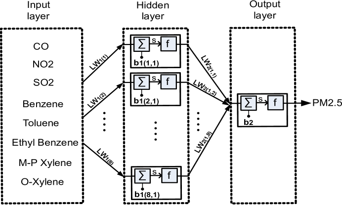
Figure 7: Selected ANN Topology for Prediction

5 Prediction model of PM2.5

In the proposed prediction model (see Fig. 7), inputs are selected based on the correlation results [Step IV]. As can be seen from Table 1, a higher correlation ($>$0.8) of CO, NO₂, SO₂, and VOC (Benzene, Toluene, Ethyl Benzene, M+P Xylene, O-Xylene) with PM2.5 is observed. So, out of 12 parameters 8 parameters; CO, NO₂, SO₂, and VOC (Benzene, Toluene, Ethyl Benzene, M+P Xylene, O-Xylene) are selected for developing the PM2.5 prediction model. Additionally, as the number of input parameters is reduced from 12 to 8, the computation cost of the proposed prediction model is reduced. The prediction model of PM2.5 shown in Fig. 7 is based on a feed-forward neural network with a single hidden layer [Step V]. Selected eight pollutants are the input parameters for each neuron of the hidden layer which consists of eight neurons.

The weights of the hidden layer and output layer can be represented by a matrix of size $S\times P$, where, $S$ is equal to the number of neurons in the layer and $P$ is equal to the number of inputs of the layer. In our case, the matrix size is 8$\times$8, as both the inputs and hidden layer size are 8. The matrix size for the output layer is 1$\times$8 as it consists of one neuron and eight inputs coming from the hidden layer. For the proposed predicted model, weights of the hidden layer and output layer are represented by LW₁ of (of 8$\times$8 size) and LW₂ of size (of 1$\times$8 size) respectively. The element, LW₁(1) represents the first row of LW₁ matrix, which is formed by the weights of inputs going to the first neuron of the hidden layer. Similarly, LW₂(1,1) represents the first row and first column element of matrix LW₂ and so on. Biases of the particular layer can be represented by a matrix of the size S$\times$1, where S is equal to the number of neurons in the layer. The bias matrices are b₁ and b₂ for hidden layer and output layer, respectively. As the number of neurons in the hidden layer is 8 and output layer is 1, the bias matrices, b₁ is 8$\times$1 and b₂ is 1$\times$1, where b₁(1,1) represents the first row and first column element of matrix b₁.

The training function trainlm based on the Levenberg-Marquardt algorithm is adopted sharma2014comparison ; mathtrain for training. To train the network for the nonlinear relationship between input and output and to constrain output in positive range standard nonlinear transfer function logsig given by Eq. (4) is used in the hidden layer.

$$logsig(m)=\dfrac{1}{(1+e^{-m})}$$ (4)

where m is the input to the transfer function. In logsig transfer function, the output will be in the range of [0:1] for the entire range of inputs. For nonlinear regression or prediction, purelin is an effective transfer function for the output layer ref4 . Hence in the proposed model, purelin is used as a transfer function in the output layer. In purelin, the output will be equal to the input.

The total available data of 18k+ is divided into two sets the first set (SET1) includes 90% of data and the second set (SET2) includes 10% of data [Step VI]. The division into two sets is done randomly so that all types of data can be included in two sets. The SET1 (90% data) is used for designing the neural network and it is divided in a standard manner widely used by researchers, 70% for training, 15% for validating and 15% for testing. The SET2 (10% data) is kept as unseen data for further testing and comparing the performance of neural networks.

1:Load the data SET1 for developing the network and SET2 to test the Network for unseen data

2:for i = 1 to 100 do

3:      Divide SET1 randomly for training(70%), validating(15%) and testing (15%)

4:     Initialize the weights and biases

5:     Train the network

6:     Validate the network

7:     Test the network

8:     Evaluate training, validation and testing performance

9:     Save the performance results

10:     Save Network and its weights and biases

11:      Test the Network performance for unseen data using SET2

12:     Save the performance results

13:end for

Algorithm 1 Pseudo Code for Developing and Testing 100 different ANNs

For selecting the best ANN for prediction model, 100 different ANNs are developed and tested as per the pseudo-code in Algorithm 1. This algorithm is repeated 100 times to get the performance of 100 different ANNs for comparing training and testing results with good generalization [Step VII, VIII]. The performance of the ANN is evaluated [Step IX] based on, RMSE and R², where, RMSE is the root mean square of the errors, i.e, the difference between the target value and the predicted value and is given in Eq. (5).

$$RMSE=\sqrt{\dfrac{\sum_{i=1}^{n}(A_{i}-P_{i})^{2}}{n}}$$ (5)

where A_i represents the actual value, P_i represents the predicted value and n is the total number of samples. R² is the coefficient of determination and it is the square of the correlation R (Eq. (1)). The closeness between target values and predicted outputs of ANN is represented by R². The value of R² equal to 1 represents targets and predicted outputs are very close to each other.

5.0.1 Model Equations

The hidden layer and output layer weights for the proposed model are shown in Eq. (6) and Eq. (7) respectively. The biases of the model for hidden layer and output layer are shown in Eq. (8) and Eq. (9) respectively. Matrix B₁ is formed by repeating the hidden layer bias matrix b₁, N times, where N is equal to the size of test dataset (1838 in our case). This operation shown in Eq. (10), is performed to make bias matrix size B₁ equal to the size of product term matrix $LW_{1}$*$x_{n}$, so that addition operation (B₁ + $LW_{1}$*$x_{n}$), shown in Eq. (11) can be performed.

$$LW_{1}=\left[\begin{matrix}-25.978&-31.063&17.505&38.446&-37.353&97.708&-92.951&65.964\\ 3.295&6.460&0.203&-1.981&10.078&-10.281&3.352&-3.782\\ -2.661&2.503&-1.075&-1.011&-0.194&1.702&-2.768&1.690\\ -6.069&6.142&-2.212&-3.593&1.800&-3.002&0.222&2.803\\ -9.788&-7.748&-4.424&27.227&-4.406&0.016&-6.279&8.460\\ 3.821&-6.233&1.243&-1.449&5.600&1.846&1.801&-5.862\\ 3.149&6.319&0.368&-0.825&10.746&-11.220&2.650&-3.428\\ -2.127&1.991&-1.116&-0.032&0.038&4.094&-4.882&1.330\\ \end{matrix}\right]$$ (6)

$$LW_{2}=\left[\begin{matrix}0.158&-17.591&-6.481&1.614&-0.369&-0.817&17.345&4.950\\ \end{matrix}\right]$$ (7)

$$b_{1}=\left[\begin{matrix}34.474\\ 4.001\\ -1.015\\ -2.615\\ 5.700\\ -0.148\\ 4.383\\ -1.959\\ \end{matrix}\right]$$ (8)

$$b_{2}=\left[\begin{matrix}1.593\\ \end{matrix}\right]$$ (9)

$$B_{1}=\left[\begin{matrix}b_{1}&b_{1}&b_{1}&b_{1}&.&.&.&.&.&N\end{matrix}\right]$$ (10)

The prediction model for deriving PM2.5 [Step X] is given by Eq. (11).

$$PM2.5_{n}=b_{2}+LW_{2}*logsig(B_{1}+LW_{1}*x_{n})$$ (11)

where PM2.5_n is normalized output. The input matrix x_n is formed using normalized values of CO, NO₂, SO₂, and VOC and the size of x_n is $P\times N$ where $P$=8 is the number of inputs and $N$=1838 is the number of values for each input. Eq. (11) shows the usefulness of the approach to obtain the value of PM2.5 based on CO, NO₂, SO₂, and VOC values only. Therefore, low-cost sensors can be deployed with the derived model that offers the opportunity to derive PM2.5 through signal processing algorithms. Eq. (12) shows the conversion to the original value from the normalized one using Eq. (3), in which X_max and X_min are taken as per Fig. 6.

$$PM2.5=\dfrac{(PM2.5_{n}+1)*(180.052-2.228)}{2}+2.228$$ (12)

The proposed approach based on the above analytical equations eliminates the need for proprietary tools. The analytical equation for the prediction can be computed using any low-cost processing tool (e.g. excel sheet etc.). A screenshot of an example [Step XI] is shown in Fig. 8. In this example, an input matrix x of size 8$\times$1838 is taken which represents the testing data set. Eq. (11) is computed as follows.

1. First, $x_{n}$ is obtained by computing Eq. (2)

2. Multiplying the two matrices of $LW_{1}$ (Eq. (6)) and $x_{n}$, product term $LW_{1}$*$x_{n}$ is obtained.

3. Matrix $B_{1}$, formed using Eq. (10) is added in the product term $LW_{1}$*$x_{n}$.

4. Hidden layer activation function (Eq. (4)) is applied to find the output of the hidden layer.

5. The output of the hidden layer is multiplied by $LW_{2}$ (Eq. (7)).

6. Then matrix $b_{2}$ from Eq. (9), is added.

Finally, PM2.5_n (marked as in Fig. 8) is obtained by computing Eq. (11), which is the normalized value of PM2.5. PM2.5 in the original unit is obtained by processing Eq. (12) (marked as in Fig. 8). Predicted values of PM2.5 obtained from Eq. (12) (marked as in Fig. 8) are close to the actual values of PM2.5 (marked as in Fig. 8). Interestingly these computations can be ported to a wireless sensor node having basic memory along with computational capability and the algorithms can still perform reliably.

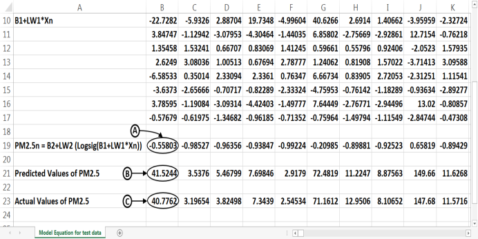
Figure 8: Excel sheet used for processing prediction model equation

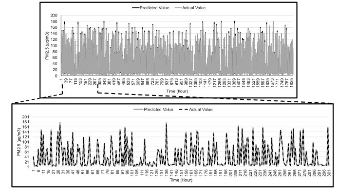
Figure 9: Good match of the results obtained from the analytical equation of model with actual values

The deployment of the developed prediction model needs to consider the following limitations based on the location, available monitoring stations and available monitoring parameters as predictors.

• Air pollution varies from one location to another based on the few parameters like human activity, traffic condition, the structure of urban area and weather conditions. Based on the location, predictors and predictand values as well as their maximum and the minimum limit will change. So, the application of the presented prediction model for another location needs model training, validation, and testing again which provides new coefficients in terms of weights and biases for accurate prediction with lower RMSE.

• Application of prediction model to another location requires a large set of authentic data for training which is sometimes difficult due to the limitation on the number of online environment monitoring stations. Due to a few monitoring parameters, and delay in the availability of data; offline stations are less preferable than online stations.

• Online stations of CPCB monitors pollutants that are greater than the offline stations. Concentration data for a large set of pollutants is the basic requirement for a correlation study or developing a prediction model. Due to the limitation on the online stations available in the city, data were used from only one online station for training, validation, and testing in the proposed study. This can be expanded in the future by taking data from multiple online stations of different cities.

• The derived prediction model based on ANN generally shows poor performance for predicting the sudden large change in predictors. As, sometimes it is difficult to discriminate between the outliers and sudden change in the value, applying a smoothing algorithm to remove outliers will also remove the sudden large change in the value of the predictor. This limitation can be targeted through different data processing algorithm and is left as part of future work

5.0.2 Model Results

In comparison to Support Vector Machine (SVM), the ANN exhibits better performance in terms of RMSE. The RMSE of 2.862 and 2.823 is obtained during training and testing respectively for the SVM model (shown in Table 2). While for ANN, the RMSE of 1.5971 and 1.5121 is obtained (shown in Table 3) during training and testing for unseen data respectively.

Table 2: Performance of SVM

Performance of	RMSE
Training	2.862
Testing for unseen data	2.823

Table 3: Performance of Prediction Model

Performance of	RMSE	R2
Training	1.5971	0.9987
Validation	1.6347	0.9986
Testing	1.5843	0.9988
Testing for unseen data	1.5121	0.9988

Table 3 shows the best performance of the prediction model obtained from 100 iterations. The value of R² demonstrates the closeness of the predicted values with the target values or actual values. The actual values of PM2.5 are compared (see Fig. 9) with predicted results obtained by Eq. (12). It is found that the predicted results are in close accordance with actual values, which confirms the effectiveness of the proposed approach.

Table 4: Summary of previously developed prediction models

Reference	Predictand	RMSE	R2
lu2006prediction	O3 (ppb)	0.30	0.69
Sousa2007	O3 (µg/m3)	21.78	0.73
gardner1999neural	NO2 (ppb)	7.3	0.91
A2006	NO2 (µg/m3)	13.93	0.93
grivas2006artificial	PM 10 (µg/m3)	12.16	0.83
diaz2008hybrid	PM 10 (µg/m3)	11.656	0.983
nc8	PM2.5 (µg/m3)	41.97	-
ann25	PM2.5 (µg/m3)	12.8903	-
ann5	PM10 (µg/m3)	18.4	0.895
ann5	PM2.5 (µg/m3)	12.7	0.954
ann6	PM2.5 (µg/m3)	6.77	0.99
hybrid6	PM2.5 (µg/m3)	5.0324	0.79
corr27	PM2.5 (µg/m3)	14.47	-
corr7	PM2.5 (µg/m3)	24.06	-
everyaware	BC (ng/m3)	1480.746	0.586
This Work	PM2.5 (µg/m3)	1.7973	0.9986

Previously developed prediction models, depend on past data, are often time-consuming and use dedicated instruments. In the prediction model, we have eliminated the above requirements and comparison with some researches is shown in Table 4. As can be seen, the proposed approach has better RMSE and R² compared to existing methods. The RMSE of 1.7973 µg/m³ and R² of 0.9986 is obtained for test dataset of size 1838. We extended the model to accommodate a reduced test dataset of size 10, which shows RMSE of 146.10 µg/m³ and R² of 0.9467. The proposed model in the form of the analytical equation thus helps in predicting PM2.5 using low-cost processing tools or existing WSN.

The proposed prediction model is recalibrated in terms of the number of predictors, weights, and biases to show the effectiveness of the proposed approach. Instead of eight predictors, three predictors, CO, NO₂, and Benzene (VOC component) are taken considering the availability of low-cost sensors mics6814 which includes this type of multiple sensing parameters. The proposed approach can work for any other three sensing parameters after recalibrating model. In recalibration, CPCB smoothed data for CO, NO₂, and Benzene (VOC component) are used as it is considered as golden standard data. For recalibration ANN shown in Fig. 7 is used with the same training and testing dataset (of three parameters), but the size of the input layer and the hidden layer is reduced to three. Extracted weights and biases are represented in Eq. (13) to Eq. (16). Performance results are shown in Table 5. Results show, during testing RMSE is 7.5372 µg/m³ and R² is 0.9708.

$$LW_{1}=\left[\begin{matrix}26.281&3.456&-12.391\\ 17.898&-0.863&11.305\\ -0.996&-0.502&-1.205\\ \end{matrix}\right]$$ (13)

$$LW_{2}=\left[\begin{matrix}-1.008&1.379&-1.665\\ \end{matrix}\right]$$ (14)

$$b_{1}=\left[\begin{matrix}9.934\\ 21.939\\ 1.101\\ \end{matrix}\right]$$ (15)

$$b_{2}=\left[\begin{matrix}0.689\\ \end{matrix}\right]$$ (16)

Table 5: Performance of Prediction Model for Three Predictors

Performance of	RMSE	R2
Training	7.9297	0.9678
Validation	8.0954	0.9679
Testing	8.0049	0.9672
Testing for unseen data	7.5372	0.9708

6 Conclusion and Future Work

In this work, we have studied the correlation of PM2.5 with other pollutants and correlation among the pollutants, based on the standardized CPCB data. The prediction model of PM2.5 is based on the correlation and shown to be useful for online as well as offline measurements. The proposed model is in the form of analytical equations that enables the use of any low-cost processing tool and eliminates the need for a proprietary tool for predicting PM2.5 values. Results obtained using this method with eight predictors ( NO₂, SO₂, and VOC (Benzene, Toluene, Ethyl Benzene, M+P Xylene, O-Xylene)) shows RMSE of 1.7973µg/m³ and R² 0.9986 for the test dataset. To show the effectiveness of the proposed approach, the derived prediction model was recalibrated with three predictors (CO, NO₂, and Benzene (VOC component) due to the possibility of sensing all three parameters by one or two low-cost sensors. The proposed approach can work for any other three sensing parameters too after recalibration. Testing results show RMSE of 7.5372 µg/m³ and R² of 0.9708. The obtained results prove the effectiveness of the proposed approach. The obtained results can be improved in the future by recalibrating prediction model based on the data available from multiple stations located at the place of deployment. In comparison to existing methods, the proposed approach facilitates an efficient method that reduces overall computation cost. Furthermore, this model can be implemented on the wireless sensor node for automated measurement of PM2.5.

7 Acknowledgement

The authors thank the Central Pollution Control Board (CPCB) and their staff for their support during this research work.

Compliance with ethical standards

Conflict of interest: The authors declare that they have no conflict of interest.

References

- (1) Central Pollution Control Board (2019) Air quality monitoring, Emission Inventory and Source Apportionment Studies for Indian Cities. https://cpcb.nic.in/source-apportionment-studies/. Accessed 4 January 2019
- (2) United States Environmental Protection Agency (2019) Pollutants and Sources. https://www3.epa.gov/ttn/atw/pollsour.html. Accessed 2 January 2019
- (3) Central Pollution Control Board (2019) National Air Quality Monitoring Programme. http://cpcb.nic.in/about-namp/. Accessed 10 January 2019
- (4) Central Pollution Control Board (2018) National Air Quality Index.http://www.indiaenvironmentportal.org.in/files/file/Air%20Quality%20Index.pdf. Accessed 25 December 2018
- (5) Central Pollution Control Board (2018) How is AQI Calculated. https://app.cpcbccr.com/ccr_docs/How_AQI_Calculated.pdf. Accessed 24 September 2018
- (6) World Health Organization (2018) Health Effects of Particulate Matter. http://www.euro.who.int/__data/assets/pdf_file/0006/189051/Health-effects-of-particulate-matter-final-Eng.pdf. Accessed 20 December 2018
- (7) Hodan WM, Barnard WR (2004) Evaluating the Contribution of PM2.5 Precursor Gases and Re-Entrained Road Emissions to Mobile Source PM2.5 Particulate Matter Emissions. MACTEC Federal Programs, Research Triangle Park, NC
- (8) Amaral S, de Carvalho J, Costa M, Pinheiro C (2015) An Overview of Particulate Matter Measurement Instruments. Atmosphere 6(9):1327-45.
- (9) Budde M, Zhang L, Beigl M (2014) Distributed, Low-Cost Particulate Matter Sensing: Scenarios, Challenges, Approaches. ProScience 1:230-6
- (10) Central Pollution Control Board (2011) Guidelines for the Measurement of Ambient Air Pollutants Volume-II.http://www.indiaenvironmentportal.org.in/files/NAAQSManualVolumeII.pdf. Accessed 2 December 2018
- (11) Environment S.A (2019) MP101M – Continuous, Automatic PM10, PM2.5, PM1, TSP Particulate Monitor. http://www.environnement-sa.com/products-page/en/air-quality-monitoring-en/mp101m-continuous-automatic-pm10-pm2-5-pm1-tsp-particulate-monitor/. Accessed 6 January 2019
- (12) Vilcassim MR, Thurston GD, Peltier RE, Gordon T (2014) Black Carbon and Particulate Matter (PM2.5) Concentrations in New York City’s Subway Stations. Environmental Science and Technology 48(24):14738-45
- (13) Gehrig R, Buchmann B (2003) Characterising Seasonal Variations and Spatial Distribution of Ambient PM10 and PM2.5 Concentrations based on Long-Term Swiss Monitoring Data. Atmospheric Environment 37(19):2571-80
- (14) Northcross A, Chowdhury Z, McCracken J, Canuz E, Smith KR (2010) Estimating Personal PM2.5 Exposures using CO Measurements in Guatemalan Households Cooking with Wood Fuel. Journal of Environmental Monitoring 12(4):873-8
- (15) Querol X, Alastuey A, Rodriguez S, Plana F, Mantilla E, Ruiz CR (2001) Monitoring of PM10 and PM2.5 around Primary Particulate Anthropogenic Emission Sources. Atmospheric Environment 35(5):845-58
- (16) Hall J, Loo SM, Stephenson D, Butler R, Pook M, Kiepert J, Anderson J, Terrell N (2012). A Portable Wireless Particulate Sensor System for Continuous Real-Time Environmental Monitoring. In: 42nd International Conference on Environmental Systems, pp 1-14
- (17) Mansour S, Nasser N, Karim L, Ali A (2014) Wireless Sensor Network-based Air Quality Monitoring System. In: IEEE International Conference on Computing, Networking and Communications, pp 545-550
- (18) Kasar AR, Khemnar DS, Tembhurnikar NP (2013) WSN based Air Pollution Monitoring System. International Journal of Science and Engineering Applications 2(4):55-9
- (19) Liu JH, Chen YF, Lin TS, Lai DW, Wen TH, Sun CH, Juang JY, Jiang JA (2011) Developed Urban Air Quality Monitoring System based on Wireless Sensor Networks. In: IEEE international conference on Sensing technology, pp 549-554
- (20) Yi W, Lo K, Mak T, Leung K, Leung Y, Meng M (2015) A Survey of Wireless Sensor Network based Air Pollution Monitoring Systems. Sensors 15(12):31392-427
- (21) Ordieres JB, Vergara EP, Capuz RS, Salazar RE (2005) Neural Network Prediction Model for Fine Particulate Matter (PM2.5) on the US–Mexico Border in El Paso (Texas) and Ciudad Juárez (Chihuahua). Environmental Modelling and Software 20(5):547-59
- (22) Hooyberghs J, Mensink C, Dumont G, Fierens F, Brasseur O (2005) A Neural Network Forecast for Daily Average PM10 Concentrations in Belgium. Atmospheric Environment 39(18):3279-89
- (23) Lv B, Cobourn WG, Bai Y (2016). Development of Nonlinear Empirical Models to Forecast Daily PM2. 5 and Ozone Levels in Three Large Chinese Cities. Atmospheric Environment 147:209-23
- (24) Perez P, Gramsch E (2016) Forecasting Hourly PM2. 5 in Santiago De Chile with Emphasis on Night Episodes. Atmospheric Environment 124:22-7
- (25) Lu HC, Hsieh JC, Chang TS (2006) Prediction of Daily Maximum Ozone Concentrations from Meteorological Conditions using a Two-Stage Neural Network. Atmospheric Research 81(2):124-39
- (26) Sousa SI, Martins FG, Alvim-Ferraz MC, Pereira MC (2007) Multiple Linear Regression and Artificial Neural Networks based on Principal Components to Predict Ozone Concentrations. Environmental Modelling and Software 22(1):97-103
- (27) Gardner MW, Dorling SR (1999) Neural Network Modelling and Prediction of Hourly NOx and NO2 Concentrations in Urban Air in London. Atmospheric Environment 33(5):709-19
- (28) Grivas G, Chaloulakou A (2006) Artificial Neural Network Models for Prediction of PM10 Hourly Concentrations, in the Greater Area of Athens, Greece. Atmospheric environment 40(7):1216-29
- (29) Chen B, Wang X, Yu L, Wang H, Li Y, Chen J, Zhu J, Nan H, Hou L (2016) Prediction of PM2.5 Concentration in a Agricultural Park Based on BP Artificial Neural Network. Advance Journal of Food Science and Technology 11(4):274-80
- (30) Biancofiore F, Busilacchio M, Verdecchia M, Tomassetti B, Aruffo E, Bianco S, Di Tommaso S, Colangeli C, Rosatelli G, Di Carlo P (2017). Recursive Neural Network Model for Analysis and Forecast of PM10 and PM2.5. Atmospheric Pollution Research 8(4):652-9
- (31) Fu M, Wang W, Le Z, Khorram MS (2015) Prediction of Particular Matter Concentrations by Developed Feed-Forward Neural Network with Rolling Mechanism and Gray Model. Neural Computing and Applications 26(8):1789-97
- (32) Chen Y (2018) Prediction Algorithm of PM2.5 Mass Concentration based on Adaptive BP Neural Network. Computing :1-4
- (33) Wang X, Wang B (2018) Research on Prediction of Environmental Aerosol and PM2. 5 based on Artificial Neural Network. Neural Computing and Applications.:1-1.
- (34) Chelani AB, Devotta S (2006) Air Quality Forecasting using a Hybrid Autoregressive and Nonlinear Model. Atmospheric Environment 40(10):1774-80
- (35) Samia A, Kaouther N, Abdelwahed T (2012) A Hybrid ARIMA and Artificial Neural Networks Model to Forecast Air Quality in Urban Areas: Case of Tunisia. Advanced Materials Research 518:2969-2979
- (36) Liu DJ, Li L (2015) Application Study of Comprehensive Forecasting Model based on Entropy Weighting Method on Trend of PM2.5 Concentration in Guangzhou, China. International Journal of Environmental Research and Public Health 12(6):7085-99
- (37) Mahajan S, Liu HM, Tsai TC, Chen LJ (2018) Improving the Accuracy and Efficiency of PM2. 5 Forecast Service Using Cluster-Based Hybrid Neural Network Model. IEEE Access 6:19193-204
- (38) Wang P, Zhang H, Qin Z, Zhang G (2017) A Novel Hybrid-Garch Model based on ARIMA and SVM for PM2. 5 concentrations forecasting. Atmospheric Pollution Research 8(5):850-60
- (39) Feng X, Li Q, Zhu Y, Hou J, Jin L, Wang J (2015) Artificial Neural Networks Forecasting of PM2.5 Pollution using Air Mass Trajectory based Geographic Model and Wavelet Transformation. Atmospheric Environment 107:118-28
- (40) Ausati S, Amanollahi J (2016) Assessing the Accuracy of ANFIS, EEMD-GRNN, PCR, and MLR Models in Predicting PM2. 5. Atmospheric Environment 142:465-74
- (41) Zhu D, Cai C, Yang T, Zhou X (2018) A Machine Learning Approach for Air Quality Prediction: Model Regularization and Optimization. Big Data and Cognitive Computing 2(1):5
- (42) Kleine Deters J, Zalakeviciute R, Gonzalez M, Rybarczyk Y (2017) Modeling PM2. 5 Urban Pollution using Machine Learning and Selected Meteorological Parameters. Journal of Electrical and Computer Engineering
- (43) Soh PW, Chang JW, Huang JW (2018) Adaptive Deep Learning-Based Air Quality Prediction Model using the Most Relevant Spatial-Temporal Relations. IEEE Access 6:38186-99
- (44) Lin Y, Mago N, Gao Y, Li Y, Chiang YY, Shahabi C, Ambite JL (2018) Exploiting Spatiotemporal Patterns for Accurate Air Quality Forecasting using Deep Learning. In: Proceedings of the 26th ACM SIGSPATIAL International Conference on Advances in Geographic Information Systems,pp 359-368
- (45) Li X, Peng L, Hu Y, Shao J, Chi T (2016). Deep Learning Architecture for Air Quality Predictions. Environmental Science and Pollution Research 23(22):22408-17
- (46) Sun W, Sun J (2017) Daily PM2.5 Concentration Prediction based on Principal Component Analysis and LSSVM Optimized by Cuckoo Search Algorithm. Journal of Environmental Management 188:144-52
- (47) Ni XY, Huang H, Du WP (2017) Relevance Analysis and Short-Term Prediction of PM2.5 Concentrations in Beijing based on Multi-Source Data. Atmospheric Environment 150:146-61
- (48) EveryAware (2014) Final Report on: Sensor Selection, Calibration and Testing; EveryAware Platform; Smartphone Applications. http://www.everyaware.eu/resources/deliverables/D1.2.pdf. Accessed 9 January 2019
- (49) Baby A, Alexander AA (2018) A Review on Various Techniques used in Predicting Pollutants. In IOP Conference Series: Materials Science and Engineering 396(1): 012016
- (50) Mathbits (2018) Correlation Cofficient. https://mathbits.com/MathBits/TISection/Statistics2/correlation.htm. Accessed 27 December 2018
- (51) Icopal Noxite (2019) Nitrogen Oxide (NOx) Pollution. http://www.m.icopal-noxite.co.uk/nox-problem/nox-pollution.aspx. Accessed 30 August 2019
- (52) World Health Organization (2019) Air Pollution. https://www.who.int/airpollution/ambient/pollutants/en/. Accessed 31 August 2019
- (53) European Environment Agency (2019) Some Common Air Pollutants. https://www.eea.europa.eu/publications/2599XXX/page008.html. Accessed 31 August 2019
- (54) Sharma B, Venugopalan K (2014) Comparison of Neural Network Training Functions for Hematoma Classification in Brain CT Images. IOSR Journal of Computer Engineering 16(1):31-5
- (55) The MathWorks Inc(2018) Train and Apply Multilayer Neural Networks. https://www.mathworks.com/help/deeplearning/ug/train-and-apply-multilayer-neural-networks.html. Accessed 15 September 2018
- (56) The MathWorks Inc (2019) Multilayer Shallow Neural Network Architecture. https://in.mathworks.com/help/deeplearning/ug/multilayer-neural-network-architecture.html. Accessed 30 August 2019
- (57) SGX sensortech (2019) The MICS-6814 is a Compact MOS Sensor with Three Fully Independent Sensing Elements on One Package. https://sgx.cdistore.com/datasheets/sgx/1143_Datasheet%20MiCS-6814%20rev%208.pdf. Accessed 2 January 2019