The ratio of the partial widths of some dimension-5 proton decay modes can be predicted without detailed knowledge of SUSY particle masses, and thus allows us to experimentally test various SUSY GUT models without discovering SUSY particles. In this paper, we study the ratio of the partial widths of the $p\to K^{0}\mu^{+}$ and $p\to K^{+}\bar{\nu}_{\mu}$ decays in the minimal renormalizable SUSY $SO(10)$ GUT, under only a plausible assumption that the 1st and 2nd generation left-handed squarks are mass-degenerate. In the model, we expect that the Wilson coefficients of dimension-5 operators responsible for these modes are on the same order and that the ratio of $p\to K^{0}\mu^{+}$ and $p\to K^{+}\bar{\nu}_{\mu}$ partial widths is $O(0.1)$. Hence, we may be able to detect both $p\to K^{0}\mu^{+}$ and $p\to K^{+}\bar{\nu}_{\mu}$ decays at Hyper-Kamiokande, thereby gaining a hint for the minimal renormalizable SUSY $SO(10)$ GUT. Moreover, since this partial width ratio is quite suppressed in the minimal $SU(5)$ GUT, it allows us to distinguish the minimal renormalizable SUSY $SO(10)$ GUT from the minimal $SU(5)$ GUT. In the main body of the paper, we perform a fitting of the quark and lepton masses and flavor mixings with the Yukawa couplings of the minimal renormalizable $SO(10)$ GUT, and derive a concrete prediction for the partial width ratio based on the fitting results. We find that the partial width ratio generally varies in the range 0.05-0.6, confirming the above expectation.

1 Introduction

The $SO(10)$ grand unified theory (GUT) [1, 2] is a well-motivated scenario beyond the Standard Model (SM), since it unifies the SM gauge groups into an anomaly-free group, it unifies the SM matter fields and right-handed neutrino of each generation into one 16 representation, and it includes the seesaw mechanism [3, 4, 5, 6] for the tiny neutrino mass. The minimal renormalizable $SO(10)$ GUT [7], where the electroweak-symmetry-breaking-Higgs field stems from ${\bf 10}+{\bf\overline{126}}$ fields and the SM Yukawa couplings come solely from renormalizable terms $\tilde{Y}_{10}\,{\bf 16}\,{\bf 10}\,{\bf 16}+\tilde{Y}_{126}\,{\bf 16}\,{\bf\overline{126}}\,{\bf 16}$, is even more appealing because the mass and flavor mixings of quarks and leptons are derived from a restricted set of parameters. Specifically, the up-type quark, down-type quark, charged lepton and neutrino Dirac Yukawa matrices are derived as $Y_{u}=Y_{10}+r_{2}Y_{126}$, $Y_{d}=r_{1}(Y_{10}+Y_{126})$, $Y_{e}=r_{1}(Y_{10}-3Y_{126})$, $Y_{D}=Y_{10}-3r_{2}Y_{126}$, with $Y_{10}\propto\tilde{Y}_{10}$, $Y_{126}\propto\tilde{Y}_{126}$ and $r_{1},r_{2}$ being numbers. Also, the Majorana mass for right-handed neutrinos and the type-2 seesaw contribution to the tiny neutrino mass are proportional to $Y_{126}$.

The direct experimental signature of the minimal renormalizable $SO(10)$ GUT is, like other GUT models, proton decay. In supersymmetric (SUSY) GUT, proton decay through dimension-5 operators induced by colored Higgsino exchange [8, 9] can be within the reach of Hyper-Kamiokande experiment [10] and is crucial to phenomenology. Regrettably, SUSY particles have not been discovered at the LHC and hence no concrete prediction is available for the partial widths of dimension-5 proton decays, since they are inversely proportional to the soft SUSY breaking scale squared. In this situation, the ratio of the partial widths of different decay modes, which is independent of the soft SUSY breaking scale , allows us to test various SUSY GUT models including the minimal renormalizable SUSY $SO(10)$ GUT.

In this paper, we focus on the ratio of the partial widths of the $p\to K^{0}\mu^{+}$ and the $p\to K^{+}\bar{\nu}_{\mu}$ decays in the minimal renormalizable SUSY $SO(10)$ GUT. We make only one natural assumption on the SUSY particle mass spectrum, which is that the 1st and 2nd generation left-handed squarks are mass-degenerate. In the model with the above assumption, the ratio $\Gamma(p\to K^{0}\mu^{+})/\Gamma(p\to K^{+}\bar{\nu}_{\mu})$ is predicted to be $O(0.1)$. Hence, we may be able to discover both $p\to K^{0}\mu^{+}$ and $p\to K^{+}\bar{\nu}_{\mu}$ decays at Hyper-Kamiokande [10], thereby gaining a hint for the model. Moreover, this ratio is predicted to be suppressed by factor 0.002 in the minimal $SU(5)$ GUT compared to the minimal renormalizable SUSY $SO(10)$ GUT , and thus observation of both $p\to K^{0}\mu^{+}$ and $p\to K^{+}\bar{\nu}_{\mu}$ decays allows us to distinguish the latter from the former.

In the main body of the paper, we numerically confirm that $\Gamma(p\to K^{0}\mu^{+})/\Gamma(p\to K^{+}\bar{\nu}_{\mu})$ is $O(0.1)$ in the minimal renormalizable SUSY $SO(10)$ GUT. To this end, we determine the fundamental Yukawa couplings $Y_{10},Y_{126}$ through a fitting of the quark and lepton Yukawa couplings and neutrino data, as has been performed in Refs. [12]-[30], and calculate the partial width ratio based on the fitting results.

Previously, enhancement of partial width ratio $\Gamma(p\to K^{0}\mu^{+})/\Gamma(p\to K^{+}\bar{\nu}_{\mu})$ in $SO(10)$ GUT models compared to the minimal $SU(5)$ GUT is claimed in Refs. [31, 32], but only based on a qualitative argument. Our paper is the first study where this ratio is predicted concretely and quantitatively in the minimal renormalizable SUSY $SO(10)$ GUT, with the fundamental Yukawa couplings $Y_{10},Y_{126}$ determined through a numerical fitting.

The basic reason that $\Gamma(p\to K^{0}\mu^{+})/\Gamma(p\to K^{+}\bar{\nu}_{\mu})$ is $O(0.1)$ in the minimal renormalizable SUSY $SO(10)$ GUT is understood as follows. In the model, the ratio of the Wilson coefficients of dimension-5 operators responsible for the $p\to K^{0}\mu^{+}$ decay and those for the $p\to K^{+}\bar{\nu}_{\mu}$ decay, is proportional to $(Y_{10})_{u_{L}\,j}/(Y_{10})_{d_{L}\,j}$ or $(Y_{126})_{u_{L}\,j}/(Y_{126})_{d_{L}\,j}$. Here $(Y_{10})_{u_{L}\,j}$ denotes (1,$j$)-component of $Y_{10}$ in the flavor basis where, when we write the Yukawa coupling as $\psi_{i}(Y_{10})_{ij}\psi_{j}$, the left-handed up-type quark component of $\psi_{i}$ has the diagonalized up-type quark Yukawa coupling. $(Y_{10})_{d_{L}\,j},(Y_{126})_{u_{L}\,j},(Y_{126})_{d_{L}\,j}$ are defined in the same way. $Y_{10},Y_{126}$ are linear combinations of the down-type and up-type quark Yukawa matrices $Y_{d},Y_{u}$, due to the relations $Y_{u}=Y_{10}+r_{2}Y_{126},Y_{d}=r_{1}(Y_{10}+Y_{126})$. Moreover, these linear combinations are generic, because situations where $Y_{10}\propto Y_{u},Y_{126}\propto Y_{d}$ or $Y_{10}\propto Y_{d},Y_{126}\propto Y_{u}$ would not reproduce the correct charged lepton Yukawa matrix $Y_{e}$. Therefore, considering the large hierarchy $y_{u}/y_{t}\ll y_{d}/y_{b}$, we expect that the components $(Y_{10})_{u_{L}\,j},(Y_{10})_{d_{L}\,j},(Y_{126})_{u_{L}\,j},(Y_{126})_{d_{L}\,j}$ are all on the order of the down quark Yukawa coupling $y_{d}$ times the mixing angle between the right-handed down quark and a state with flavor index $j$, and are not proportional to the up quark Yukawa coupling $y_{u}$. Hence, both $(Y_{10})_{u_{L}\,j}/(Y_{10})_{d_{L}\,j}$ and $(Y_{126})_{u_{L}\,j}/(Y_{126})_{d_{L}\,j}$ are $O(1)$ and so is the ratio of the Wilson coefficients of dimension-5 operators for the $p\to K^{0}\mu^{+}$ and the $p\to K^{+}\bar{\nu}_{\mu}$ decays. The Wino-dressing diagrams give almost the same contribution for the two modes, if the 1st and 2nd generation left-handed squarks are mass-degenerate. As a result, the partial width ratio $\Gamma(p\to K^{0}\mu^{+})/\Gamma(p\to K^{+}\bar{\nu}_{\mu})$ is determined by the ratio of baryon chiral Lagrangian parameters, which lies in the range $(1-D+F)^{2}/(1+D+F)^{2}=0.085$ to $(1-D+F)^{2}/(1-D/3+F)^{2}=0.30$, and thus the partial width ratio is $O(0.1)$.

This paper is organized as follows. In Section 2, we describe the minimal renormalizable SUSY $SO(10)$ GUT and present formulas for the partial widths of the $p\to K^{+}\bar{\nu}_{\mu}$ and $p\to K^{0}\mu^{+}$ decays. In Section 3, we roughly estimate the partial width ratio $\Gamma(p\to K^{0}\mu^{+})/\Gamma(p\to K^{+}\bar{\nu}_{\mu})$ in the minimal renormalizable SUSY $SO(10)$ GUT without numerically determining the fundamental Yukawa couplings $Y_{10},Y_{126}$, and compare it to the partial width ratio in the minimal $SU(5)$ GUT. In Section 4, we numerically determine $Y_{10},Y_{126}$ through a fitting of the quark and charged lepton Yukawa couplings and neutrino mass matrix, and calculate $\Gamma(p\to K^{0}\mu^{+})/\Gamma(p\to K^{+}\bar{\nu}_{\mu})$ based on the fitting results. Section 5 summarizes the paper.

2 Minimal Renormalizable SUSY $SO(10)$ GUT

We consider a SUSY $SO(10)$ GUT model that contains chiral superfields $H$, $\Delta$, $\overline{\Delta}$ in ${\bf 10}$, ${\bf 126}$, ${\bf\overline{126}}$ representation, and three matter fields $\Psi_{i}$ in 16 representation ($i=1,2,3$ denotes flavor index) [7]. The model also contains chiral superfields responsible for breaking $SU(5)$ subgroup of $SO(10)$, but we do not specify them in this paper. The most general renormalizable Yukawa couplings are given by

$$W_{\rm Yukawa}\ =\ (\tilde{Y}_{10})_{ij}\,\Psi_{i}H\Psi_{j}+(\tilde{Y}_{126})_{ij}\,\Psi_{i}\overline{\Delta}\Psi_{j}$$ (1)

where $(\tilde{Y}_{10})_{ij}$ and $(\tilde{Y}_{126})_{ij}$ are $3\times 3$ complex symmetric matrices. The Higgs fields of the minimal SUSY Standard Model (MSSM), $H_{u},H_{d}$, are linear combinations of (${\bf 1}$, ${\bf 2}$, $\pm\frac{1}{2}$) components of $H$, $\overline{\Delta}$ and other fields. Accordingly, the MSSM Yukawa coupling for up-type quarks, $Y_{u}$, that for down-type quarks, $Y_{d}$, and that for charged leptons, $Y_{e}$, and the Dirac Yukawa coupling for neutrinos, $Y_{D}$, are derived from $W_{\rm Yukawa}$ as

$$W_{\rm Yukawa}\ \supset\ (Y_{u})_{ij}\,Q_{i}H_{u}U_{i}^{c}+(Y_{d})_{ij}\,Q_{i}H_{d}D_{i}^{c}+(Y_{e})_{ij}\,L_{i}H_{d}E_{i}^{c}+(Y_{D})_{ij}\,L_{i}H_{u}N_{i}^{c}$$ (2)

where $Y_{u},\ Y_{d},\ Y_{e},\ Y_{D}$ are given by

$$Y_{u}\ =\ Y_{10}+r_{2}\,Y_{126},$$ (3)

$$Y_{d}\ =\ r_{1}\left(Y_{10}+Y_{126}\right),$$ (4)

$$Y_{e}\ =\ r_{1}\left(Y_{10}-3Y_{126}\right),$$ (5)

$$Y_{D}\ =\ Y_{10}-3r_{2}\,Y_{126}$$ (6)

at a $SO(10)$ breaking scale. Here $Y_{10}\propto\tilde{Y}_{10}$, $Y_{126}\propto\tilde{Y}_{126}$, and $r_{1},r_{2}$ are numbers. By a phase redefinition, we take $r_{1}$ to be real positive. In principle, $r_{1},r_{2}$ are determined from the mass matrix for (${\bf 1}$, ${\bf 2}$, $\pm\frac{1}{2}$) components [33]-[38], but in this paper we treat them as independent parameters.

Majorana mass for the right-handed neutrinos is proportional to $(Y_{126})_{ij}\,v_{R}\,N_{i}^{c}N_{j}^{c}$ where $v_{R}$ denotes $\overline{\Delta}$’s VEV. Integrating out $N_{i}^{c}$ yields an effective operator $L_{i}H_{u}L_{j}H_{u}$, which we call the Type-1 seesaw contribution. Additionally, if the (1, 3, 1) component of $\overline{\Delta}$ mixes with that of 54 representation field, after integrating out these components, we get an effective operator $L_{i}H_{u}L_{j}H_{u}$, which we call the Type-2 seesaw contribution.

$H$, $\bar{\Delta}$ and other fields contain pairs of (3, 1, $-\frac{1}{3}$), (${\bf\overline{3}}$, 1, $\frac{1}{3}$) components, which we call ‘colored Higgs fields’ and denote by $H_{C}^{A}$, $\overline{H}_{C}^{B}$ ($A,B$ are labels), respectively. Exchange of $H_{C}^{A},\overline{H}_{C}^{B}$ gives rise to dimension-5 operators inducing proton decay. Those couplings of $H_{C}^{A},\overline{H}^{B}_{C}$ which contribute to such operators are

$$W_{\rm Yukawa}\ \supset\ \sum_{A}\left[\ \frac{1}{2}(Y_{L}^{A})_{ij}\,Q_{i}H_{C}^{A}Q_{j}+(\overline{Y}^{A}_{L})_{ij}\,Q_{i}\overline{H}^{A}_{C}L_{j}+(Y_{R}^{A})_{ij}\,E^{c}_{i}H_{C}^{A}U^{c}_{j}+(\overline{Y}_{R}^{A})_{ij}\,U^{c}_{i}\overline{H}_{C}^{A}D^{c}_{j}\ \right]$$ (7)

where $Y_{L}^{A},\,\overline{Y}_{L}^{A},\,Y_{R}^{A},\,\overline{Y}^{A}_{R}$ are linear combinations of $Y_{10},\,Y_{126}$. After integrating out $H^{A}_{C},\overline{H}^{B}_{C}$, we get dimension-5 operators contributing to proton decay,

$$-W_{5}\ =\ \frac{1}{2}C_{5L}^{ijkl}\,(Q_{k}Q_{l})(Q_{i}L_{j})+C_{5R}^{ijkl}\,E^{c}_{k}U^{c}_{l}U^{c}_{i}D^{c}_{j}$$ (8)

(in the first term, isospin indices are summed in each bracket) where

$$C_{5L}^{ijkl}(\mu\sim M_{H_{C}}) =\left.\sum_{A,B}({\cal M}_{H_{C}}^{-1})_{AB}\left\{(Y_{L}^{A})_{kl}(\overline{Y}^{B}_{L})_{ij}-\frac{1}{2}(Y_{L}^{A})_{li}(\overline{Y}^{B}_{L})_{kj}-\frac{1}{2}(Y_{L}^{A})_{ik}(\overline{Y}^{B}_{L})_{lj}\right\}\right|_{\mu\sim M_{H_{C}}},$$ (9)

$$C_{5R}^{ijkl}(\mu\sim M_{H_{C}}) =\left.\sum_{A,B}({\cal M}_{H_{C}}^{-1})_{AB}\left\{(Y_{R}^{A})_{kl}(\overline{Y}_{R}^{B})_{ij}-(Y_{R}^{A})_{ki}(\overline{Y}_{R}^{B})_{lj}\right\}\right|_{\mu\sim M_{H_{C}}},$$ (10)

and ${\cal M}_{H_{C}}$ denotes the mass matrix of $H^{A}_{C},\overline{H}^{B}_{C}$ fields and $M_{H_{C}}$ represents a typical value of the eigenvalues of ${\cal M}_{H_{C}}$.

We concentrate on the contribution of the $(Q_{k}Q_{l})(Q_{i}L_{j})$ operators to the $p\to K^{+}\bar{\nu}_{\mu}$ and $p\to K^{0}\mu^{+}$ decays, and calculate the ratio of their partial widths

$$\frac{\Gamma(p\to K^{0}\mu^{+})}{\Gamma(p\to K^{+}\bar{\nu}_{\mu})}$$ (11)

in the minimal renormalizable SUSY $SO(10)$ GUT. It should be noted that the $(Q_{k}Q_{l})(Q_{i}L_{j})$ and the $E^{c}_{k}U^{c}_{l}U^{c}_{i}D^{c}_{j}$ operators contribute to the $p\to K^{+}\bar{\nu}_{\tau}$ decay, which is experimentally indistinguishable from the $p\to K^{+}\bar{\nu}_{\mu}$ decay. Hence, our prediction on $\Gamma(p\to K^{0}\mu^{+})/\Gamma(p\to K^{+}\bar{\nu}_{\mu})$ should be regarded as the maximum of the following measurable quantity:

$$\frac{\Gamma(p\to K^{0}\mu^{+})}{\sum_{i=e,\mu,\tau}\Gamma(p\to K^{+}\bar{\nu}_{i})}$$ (12)

The maximum is attained if the $(Q_{k}Q_{l})(Q_{i}L_{j})$ operators’ contribution and the $E^{c}_{k}U^{c}_{l}U^{c}_{i}D^{c}_{j}$ operators’ contribution to the $p\to K^{+}\bar{\nu}_{\tau}$ decay cancel each other. This cancellation is always possible by adjusting the ratio of the Wino mass and the $\mu$-term.

As stated in Introduction, for the SUSY particle mass spectrum, we assume that the 1st and 2nd generation left-handed squarks are mass-degenerate. To be quantitative, we assume that the 1st and 2nd generation left-handed squark masses in the up-quark-Yukawa-diagonal basis satisfy

$$|m_{\tilde{c}_{L}}^{2}-m_{\tilde{u}_{L}}^{2}|\ <\ 10^{-3}\ m_{\tilde{c}_{L}}^{2}.$$ (13)

This is a natural assumption at the quantum level, since the 1st and 2nd generation quark Yukawa couplings are tiny. To see this, note that the difference in the renormalization group corrections is given in the leading-log approximation by

$$\Delta m_{\tilde{c}_{L}}^{2}-\Delta m_{\tilde{u}_{L}}^{2}\ \simeq\ -\frac{3}{16\pi^{2}}\log\left(\frac{\Lambda^{2}}{m^{2}}\right)\left\{y_{c}^{2}-y_{u}^{2}+(Y_{d}Y_{d}^{\dagger})_{c_{L}c_{L}}-(Y_{d}Y_{d}^{\dagger})_{u_{L}u_{L}}\right\}m^{2}$$ (14)

where $m^{2}$ represents the typical scale of soft SUSY breaking masses, and $\Lambda$ denotes the scale at which initial values of the squark masses are given. We have $|y_{c}^{2}-y_{u}^{2}+(Y_{d}Y_{d}^{\dagger})_{c_{L}c_{L}}-(Y_{d}Y_{d}^{\dagger})_{u_{L}u_{L}}|<10^{-3}$ for $\tan\beta=50$ and at any renormalization scale. Hence, we get $|\Delta m_{\tilde{c}_{L}}^{2}-\Delta m_{\tilde{u}_{L}}^{2}|<1.3\times 10^{-3}\ m^{2}$ even when $\Lambda$ is the Planck scale and $m$ is 1 TeV. The tiny mass splitting assumed in Eq. (13) does not affect the results presented in the rest of the paper.

The contribution of the $C_{5L}^{ijkl}(Q_{k}Q_{l})(Q_{i}L_{j})$ term to the $p\to K^{+}\bar{\nu}_{\mu}$ and the $p\to K^{0}\mu^{+}$ decays is given by [39]

$$\Gamma(p\to K^{+}\bar{\nu}_{\mu})\ =\ {\cal C}\left|\beta_{H}(\mu_{\rm had})\frac{1}{f_{\pi}}\left\{\left(1+\frac{D}{3}+F\right)C_{LL}^{s\mu\,du}(\mu_{\rm had})+\frac{2D}{3}C_{LL}^{d\mu\,su}(\mu_{\rm had})\right\}\right|^{2},$$ (15)

$$\Gamma(p\to K^{0}\mu^{+})\ =\ {\cal C}\left|\beta_{H}(\mu_{\rm had})\frac{1}{f_{\pi}}\left(1-D+F\right)\overline{C}_{LL}^{u\mu\,us}(\mu_{\rm had})\right|^{2}$$ (16)

where ${\cal C}=\frac{m_{N}}{64\pi}\left(1-\frac{m_{K}^{2}}{m_{N}^{2}}\right)^{2}$, $\beta_{H}$ denotes a hadronic matrix element, $D,F$ are parameters of the baryon chiral Lagrangian, and $C_{LL},\overline{C}_{LL}$ are Wilson coefficients of the effective Lagrangian $-{\cal L}_{6}\supset C_{LL}^{ijkl}(\psi_{u_{L}^{k}}\psi_{d_{L}^{l}})(\psi_{d_{L}^{i}}\psi_{\nu_{L}^{j}})+\overline{C}_{LL}^{ijkl}(\psi_{d_{L}^{k}}\psi_{u_{L}^{l}})(\psi_{u_{L}^{i}}\psi_{e_{L}^{j}})$ ($\psi$ denotes a SM Weyl fermion and spinor index is summed in each bracket). We have neglected the mass splittings among nucleons and hyperons. The Wilson coefficients $C_{LL},\overline{C}_{LL}$ satisfy

$$C_{LL}^{s\mu\,du}(\mu_{\rm had})=A_{LL}(\mu_{\rm had},\mu_{\rm SUSY})\frac{M_{\widetilde{W}}}{m_{\tilde{q}}^{2}}{\cal F}\,g_{2}^{2}\left(C_{5L}^{s\mu\,ud}-C_{5L}^{u\mu\,sd}\right)|_{\mu=\mu_{\rm SUSY}},$$ (17)

$$C_{LL}^{d\mu\,su}(\mu_{\rm had})=A_{LL}(\mu_{\rm had},\mu_{\rm SUSY})\frac{M_{\widetilde{W}}}{m_{\tilde{q}}^{2}}{\cal F}\,g_{2}^{2}\left(C_{5L}^{d\mu\,us}-C_{5L}^{u\mu\,ds}\right)|_{\mu=\mu_{\rm SUSY}},$$ (18)

$$\overline{C}_{LL}^{u\mu\,us}(\mu_{\rm had})=A_{LL}(\mu_{\rm had},\mu_{\rm SUSY})\frac{M_{\widetilde{W}}}{m_{\tilde{q}}^{2}}{\cal F}\,g_{2}^{2}\left(-C_{5L}^{u\mu\,us}+C_{5L}^{s\mu\,uu}\right)|_{\mu=\mu_{\rm SUSY}},$$ (19)

where ${\cal F}$ is a common loop function factor ${\cal F}=\frac{1}{x-y}(\frac{x}{1-x}\log x-\frac{y}{1-y}\log y)/16\pi^{2}+\frac{1}{x-1}(\frac{x}{1-x}\log x+1)/16\pi^{2}$ with $x=|M_{\widetilde{W}}|^{2}/m_{\tilde{q}}^{2}$ and $y=m_{\tilde{\ell}}^{2}/m_{\tilde{q}}^{2}$, and $m_{\tilde{q}}$ denotes the 1st and 2nd generation left-handed squark masses (which are assumed to be degenerate) and $m_{\tilde{\ell}}$ denotes the mass of the left-handed smuon and muon sneutrino. $A_{LL}(\mu_{\rm had},\mu_{\rm SUSY})$ accounts for renormalization group (RG) corrections in the evolution from soft SUSY breaking scale $\mu_{\rm SUSY}$ to a hadronic scale where the value of $\beta_{H}$ is reported. $C_{5L}$ are related to the colored Higgs Yukawa couplings as

$$C_{5L}^{s\mu\,ud}(\mu_{\rm SUSY})-C_{5L}^{u\mu\,sd}(\mu_{\rm SUSY})=$$

$$\ \ \ \ \ \ \ \ A_{L}(\mu_{\rm SUSY},\mu_{H_{C}})\sum_{A,B}({\cal M}_{H_{C}}^{-1})_{AB}\,\frac{3}{2}\left\{(Y_{L}^{A})_{ud}(\overline{Y}_{L}^{B})_{s\mu}-(Y_{L}^{A})_{ds}(\overline{Y}_{L}^{B})_{u\mu}\right\}|_{\mu=\mu_{H_{C}}},$$ (20)

$$C_{5L}^{d\mu\,us}(\mu_{\rm SUSY})-C_{5L}^{u\mu\,ds}(\mu_{\rm SUSY})=$$

$$\ \ \ \ \ \ \ \ A_{L}(\mu_{\rm SUSY},\mu_{H_{C}})\sum_{A,B}({\cal M}_{H_{C}}^{-1})_{AB}\,\frac{3}{2}\left\{(Y_{L}^{A})_{us}(\overline{Y}_{L}^{B})_{d\mu}-(Y_{L}^{A})_{ds}(\overline{Y}_{L}^{B})_{u\mu}\right\}|_{\mu=\mu_{H_{C}}},$$ (21)

$$C_{5L}^{u\mu\,us}(\mu_{\rm SUSY})-C_{5L}^{s\mu\,uu}(\mu_{\rm SUSY})=$$

$$\ \ \ \ \ \ \ \ A_{L}(\mu_{\rm SUSY},\mu_{H_{C}})\sum_{A,B}({\cal M}_{H_{C}}^{-1})_{AB}\,\frac{3}{2}\left\{(Y_{L}^{A})_{us}(\overline{Y}_{L}^{B})_{u\mu}-(Y_{L}^{A})_{uu}(\overline{Y}_{L}^{B})_{s\mu}\right\}|_{\mu=\mu_{H_{C}}},$$ (22)

where $A_{L}(\mu_{\rm SUSY},\mu_{H_{C}})$ accounts for RG corrections in the evolution from colored Higgs mass scale $\mu_{H_{C}}\sim M_{H_{C}}$ to soft SUSY breaking scale $\mu_{\rm SUSY}$ .

We relate the flavor-dependent part of Eqs. (20)-(22) to $Y_{10},Y_{126}$. Since $Y_{L}^{A},\overline{Y}_{L}^{A}$ are proportional to either $Y_{10}$ or $Y_{126}$, we can write without loss of generality

$$\sum_{A,B}({\cal M}_{H_{C}}^{-1})_{AB}\left\{(Y_{L}^{A})_{ud}(\overline{Y}^{B}_{L})_{s\mu}-(Y_{L}^{A})_{ds}(\overline{Y}^{B}_{L})_{u\mu}\right\}$$

$$=\frac{1}{M_{H_{C}}}\left[a\left\{(Y_{10})_{u_{L}d_{L}}(Y_{10})_{s_{L}\mu_{L}}-(Y_{10})_{d_{L}s_{L}}(Y_{10})_{u_{L}\mu_{L}}\right\}+b\left\{(Y_{10})_{u_{L}d_{L}}(Y_{126})_{s_{L}\mu_{L}}-(Y_{10})_{d_{L}s_{L}}(Y_{126})_{u_{L}\mu_{L}}\right\}\right.$$

$$\left.+c\left\{(Y_{126})_{u_{L}d_{L}}(Y_{10})_{s_{L}\mu_{L}}-(Y_{126})_{d_{L}s_{L}}(Y_{10})_{u_{L}\mu_{L}}\right\}+d\left\{(Y_{126})_{u_{L}d_{L}}(Y_{126})_{s_{L}\mu_{L}}-(Y_{126})_{d_{L}s_{L}}(Y_{126})_{u_{L}\mu_{L}}\right\}\right]$$ (23)

$$\sum_{A,B}({\cal M}_{H_{C}}^{-1})_{AB}\left\{(Y_{L}^{A})_{us}(\overline{Y}^{B}_{L})_{d\mu}-(Y_{L}^{A})_{ds}(\overline{Y}^{B}_{L})_{u\mu}\right\}$$

$$=\frac{1}{M_{H_{C}}}\left[a\left\{(Y_{10})_{u_{L}s_{L}}(Y_{10})_{d_{L}\mu_{L}}-(Y_{10})_{d_{L}s_{L}}(Y_{10})_{u_{L}\mu_{L}}\right\}+b\left\{(Y_{10})_{u_{L}s_{L}}(Y_{126})_{d_{L}\mu_{L}}-(Y_{10})_{d_{L}s_{L}}(Y_{126})_{u_{L}\mu_{L}}\right\}\right.$$

$$\left.+c\left\{(Y_{126})_{u_{L}s_{L}}(Y_{10})_{d_{L}\mu_{L}}-(Y_{126})_{d_{L}s_{L}}(Y_{10})_{u_{L}\mu_{L}}\right\}+d\left\{(Y_{126})_{u_{L}s_{L}}(Y_{126})_{d_{L}\mu_{L}}-(Y_{126})_{d_{L}s_{L}}(Y_{126})_{u_{L}\mu_{L}}\right\}\right]$$ (24)

$$\sum_{A,B}({\cal M}_{H_{C}}^{-1})_{AB}\left\{(Y_{L}^{A})_{us}(\overline{Y}^{B}_{L})_{u\mu}-(Y_{L}^{A})_{uu}(\overline{Y}^{B}_{L})_{s\mu}\right\}$$

$$=\frac{1}{M_{H_{C}}}\left[a\left\{(Y_{10})_{u_{L}s_{L}}(Y_{10})_{u_{L}\mu_{L}}-(Y_{10})_{u_{L}u_{L}}(Y_{10})_{s_{L}\mu_{L}}\right\}+b\left\{(Y_{10})_{u_{L}s_{L}}(Y_{126})_{u_{L}\mu_{L}}-(Y_{10})_{u_{L}u_{L}}(Y_{126})_{s_{L}\mu_{L}}\right\}\right.$$

$$\left.+c\left\{(Y_{126})_{u_{L}s_{L}}(Y_{10})_{u_{L}\mu_{L}}-(Y_{126})_{u_{L}u_{L}}(Y_{10})_{s_{L}\mu_{L}}\right\}+d\left\{(Y_{126})_{u_{L}s_{L}}(Y_{126})_{u_{L}\mu_{L}}-(Y_{126})_{u_{L}u_{L}}(Y_{126})_{s_{L}\mu_{L}}\right\}\right]$$ (25)

where $M_{H_{C}}$ is a typical value of the eigenvalues of ${\cal M}_{H_{C}}$, and $a,b,c,d$ are numbers common for Eqs. (23)-(25). Here $(Y_{10})_{u_{L}s_{L}}$ denotes $(1,2)$-component of $Y_{10}$ of the term $(Y_{10})_{ij}\,\Psi_{i}H\Psi_{j}$ in the flavor basis where the left-handed up-type quark component of $\Psi_{i}$ has the diagonalized up-type quark Yukawa coupling, and the left-handed down-type quark component of $\Psi_{j}$ has the diagonalized down-type quark Yukawa coupling. $(Y_{10})_{d_{L}\mu_{L}}$, $(Y_{126})_{u_{L}s_{L}}$ and others are defined analogously.

In principle, numbers $a,b,c,d$ are determined from the colored Higgs mass matrix [33]-[38]. However, as we do not specify fields responsible for breaking $SU(5)$ subgroup of $SO(10)$, we treat $a,b,c,d$ as independent $O(1)$ parameters.

We observe that each term in Eq. (25) is given by $(Y_{10})_{u_{L}\,j}/(Y_{10})_{d_{L}\,j}$ or $(Y_{126})_{u_{L}\,j}/(Y_{126})_{d_{L}\,j}$ times some term in Eqs. (23),(24), as advertised in Introduction. For example, the term $(Y_{10})_{u_{L}s_{L}}(Y_{10})_{u_{L}\mu_{L}}$ in Eq. (25) equals $(Y_{10})_{u_{L}s_{L}}/(Y_{10})_{d_{L}s_{L}}$ times the term $(Y_{10})_{d_{L}s_{L}}(Y_{10})_{u_{L}\mu_{L}}$ in Eq. (23), and also equals $(Y_{10})_{u_{L}\mu_{L}}/(Y_{10})_{d_{L}\mu_{L}}$ times the term $(Y_{10})_{u_{L}s_{L}}(Y_{10})_{d_{L}\mu_{L}}$ in Eq. (24).

3 Estimates on $\Gamma(p\to K^{0}\mu^{+})/\Gamma(p\to K^{+}\bar{\nu}_{\mu})$

We estimate $\Gamma(p\to K^{0}\mu^{+})/\Gamma(p\to K^{+}\bar{\nu}_{\mu})$ in the minimal $SU(5)$ GUT and in the minimal renormalizable SUSY $SO(10)$ GUT without numerically determining $Y_{10},Y_{126}$. In the minimal $SU(5)$ GUT, we assume, as usual, that the splitting between the down-type quark Yukawa coupling $Y_{d}$ and the charged lepton Yukawa coupling $Y_{e}$ is realized by non-renormalizable terms.

3.1 Estimate in the Minimal $SU(5)$ GUT

In the minimal $SU(5)$ GUT, we have only one pair of colored Higgs fields, and $Y_{L}$ and $\overline{Y}_{L}$ are proportional to the Yukawa couplings for ${\bf 5}$ and ${\bf\overline{5}}$ Higgs fields, respectively. Hence, Eqs. (23)-(25) are altered to

$$\sum_{A,B}({\cal M}_{H_{C}}^{-1})_{AB}\left\{(Y_{L}^{A})_{ud}(\overline{Y}^{B}_{L})_{s\mu}-(Y_{L}^{A})_{ds}(\overline{Y}^{B}_{L})_{u\mu}\right\}=\frac{1}{M_{H_{C}}}\left\{(Y_{5})_{u_{L}d_{L}}(Y_{\overline{5}})_{s_{L}\mu_{L}}-(Y_{5})_{d_{L}s_{L}}(Y_{\overline{5}})_{u_{L}\mu_{L}}\right\}$$ (26)

$$\sum_{A,B}({\cal M}_{H_{C}}^{-1})_{AB}\left\{(Y_{L}^{A})_{ud}(\overline{Y}^{B}_{L})_{s\mu}-(Y_{L}^{A})_{ds}(\overline{Y}^{B}_{L})_{u\mu}\right\}=\frac{1}{M_{H_{C}}}\left\{(Y_{5})_{u_{L}s_{L}}(Y_{\overline{5}})_{d_{L}\mu_{L}}-(Y_{5})_{d_{L}s_{L}}(Y_{\overline{5}})_{u_{L}\mu_{L}}\right\}$$ (27)

$$\sum_{A,B}({\cal M}_{H_{C}}^{-1})_{AB}\left\{(Y_{L}^{A})_{us}(\overline{Y}^{B}_{L})_{u\mu}-(Y_{L}^{A})_{uu}(\overline{Y}^{B}_{L})_{s\mu}\right\}=\frac{1}{M_{H_{C}}}\left\{(Y_{5})_{u_{L}s_{L}}(Y_{\overline{5}})_{u_{L}\mu_{L}}-(Y_{5})_{u_{L}u_{L}}(Y_{\overline{5}})_{s_{L}\mu_{L}}\right\}$$ (28)

where $Y_{5}$ and $Y_{\overline{5}}$ denote the Yukawa couplings for ${\bf 5}$ and ${\bf\overline{5}}$ Higgs fields, respectively, and $M_{H_{C}}$ denotes the mass for the colored Higgs fields.

The key fact is that since $Y_{5}$ is identical to the up-type quark Yukawa coupling matrix, the components of $Y_{5}$ with flavor index $u_{L}$ are given by the up quark Yukawa coupling times a mixing angle. Hence, they are estimated to be

$$(Y_{5})_{u_{L}u_{L}},\ (Y_{5})_{u_{L}d_{L}} \sim y_{u}(\mu=\mu_{H_{C}})$$ (29)

$$(Y_{5})_{u_{L}s_{L}} \sim y_{u}(\mu=\mu_{H_{C}})\cdot\lambda$$ (30)

where $\mu_{H_{C}}\sim M_{H_{C}}$, and $\lambda$ denotes the Cabibbo angle $\lambda\simeq|V_{us}|\simeq|V_{cd}|\simeq 0.22$. On the other hand, $(Y_{5})_{d_{L}s_{L}}$ is estimated to be the second generation Yukawa coupling times a mixing angle as

$$(Y_{5})_{d_{L}s_{L}}\ \sim\ y_{c}(\mu_{H_{C}})\cdot\lambda$$ (31)

Although the unification of down-type quark Yukawa coupling and charged lepton Yukawa coupling is unsuccessful at the renormalizable level (but the unification can always be achieved with non-renormalizable terms), we can estimate components of $Y_{\overline{5}}$ as

$$(Y_{\overline{5}})_{s_{L}\mu_{L}} \sim y_{s}(\mu_{H_{C}})\ \ {\rm or}\ \ y_{\mu}(\mu_{H_{C}}),$$ (32)

$$(Y_{\overline{5}})_{u_{L}\mu_{L}}\ \sim\ (Y_{\overline{5}})_{d_{L}\mu_{L}} \sim y_{s}(\mu_{H_{C}})\cdot\lambda\ \ {\rm or}\ \ y_{\mu}(\mu_{H_{C}})\cdot\lambda.$$ (33)

From formulas Eqs. (15)-(22) and estimates Eqs. (26)-(33), we estimate the partial widths as

$$\Gamma(p\to K^{+}\bar{\nu}_{\mu})\ =\ {\cal C}\,\left|(1+\frac{D}{3}+F)c_{1}\,\lambda^{2}\,y_{c}\,y_{\mu}+\frac{2D}{3}c_{2}\,\lambda^{2}\,y_{c}\,y_{\mu}\right|^{2}$$ (34)

$$\Gamma(p\to K^{0}\mu^{+})\ =\ {\cal C}\,\left|(1-D+F)c_{3}\,y_{u}\,y_{\mu}\right|^{2}$$ (35)

or

$$\Gamma(p\to K^{+}\bar{\nu}_{\mu})\ =\ {\cal C}\,\left|(1+\frac{D}{3}+F)c_{1}\,\lambda^{2}\,y_{c}\,y_{s}+\frac{2D}{3}c_{2}\,\lambda^{2}\,y_{c}\,y_{s}\right|^{2}$$ (36)

$$\Gamma(p\to K^{0}\mu^{+})\ =\ {\cal C}\,\left|(1-D+F)c_{3}\,y_{u}\,y_{s}\right|^{2}$$ (37)

where ${\cal C}$ is a common constant, $c_{1},c_{2},c_{3}$ are $O(1)$ numbers, and $y_{u},y_{c},y_{\mu},y_{s}$ are the up, charm, muon and strange quark Yukawa couplings at scale $\mu=\mu_{H_{C}}$. We have discarded subleading terms. The partial width ratio is then estimated as

$$\left(\frac{1-D+F}{1+D+F}\right)^{2}\left(\frac{y_{u}}{\lambda^{2}y_{c}}\right)^{2}\ \lesssim\ \frac{\Gamma(p\to K^{0}\mu^{+})}{\Gamma(p\to K^{+}\bar{\nu}_{\mu})}\ \lesssim\ \left(\frac{1-D+F}{1-D/3+F}\right)^{2}\left(\frac{y_{u}}{\lambda^{2}y_{c}}\right)^{2}$$ (38)

where the variation is due to unknown relative phase between $c_{1}$ and $c_{2}$. Numerically, the above estimate becomes

$$\left(\frac{1-D+F}{1+D+F}\right)^{2}\cdot 0.002\ \lesssim\ \frac{\Gamma(p\to K^{0}\mu^{+})}{\Gamma(p\to K^{+}\bar{\nu}_{\mu})}\ \lesssim\ \left(\frac{1-D+F}{1-D/3+F}\right)^{2}\cdot 0.002.$$ (39)

We find that $p\to K^{0}\mu^{+}$ partial width is quite suppressed compared to $p\to K^{+}\bar{\nu}_{\mu}$ partial width because of the factor 0.002 coming from the ratio of $y_{u}$ and $\lambda^{2}y_{c}$, namely, the large hierarchy between the up and charm quark Yukawa couplings suppresses the partial width ratio. Also, baryon chiral Lagrangian parameters give $(1-D+F)^{2}/(1+D+F)^{2}=0.085$ and $(1-D+F)^{2}/(1-D/3+F)^{2}=0.3$, and they provide further suppression.

3.2 Estimate in the Minimal Renormalizable SUSY $SO(10)$ GUT

In the minimal renormalizable SUSY $SO(10)$ GUT, we can rewrite the right-hand side of Eqs. (23)-(25) using the relation $Y_{u}=Y_{10}+r_{2}\,Y_{126}$, as

$$\sum_{A,B}({\cal M}_{H_{C}}^{-1})_{AB}\left\{(Y_{L}^{A})_{ud}(\overline{Y}^{B}_{L})_{s\mu}-(Y_{L}^{A})_{ds}(\overline{Y}^{B}_{L})_{u\mu}\right\}$$

$$=\frac{1}{M_{H_{C}}}\left[a\left\{(Y_{u})_{u_{L}d_{L}}(Y_{u})_{s_{L}\mu_{L}}-(Y_{u})_{d_{L}s_{L}}(Y_{u})_{u_{L}\mu_{L}}\right\}+b^{\prime}\left\{(Y_{u})_{u_{L}d_{L}}(Y_{126})_{s_{L}\mu_{L}}-(Y_{u})_{d_{L}s_{L}}(Y_{126})_{u_{L}\mu_{L}}\right\}\right.$$

$$\left.+c^{\prime}\left\{(Y_{126})_{u_{L}d_{L}}(Y_{u})_{s_{L}\mu_{L}}-(Y_{126})_{d_{L}s_{L}}(Y_{u})_{u_{L}\mu_{L}}\right\}+d^{\prime}\left\{(Y_{126})_{u_{L}d_{L}}(Y_{126})_{s_{L}\mu_{L}}-(Y_{126})_{d_{L}s_{L}}(Y_{126})_{u_{L}\mu_{L}}\right\}\right]$$ (40)

$$\sum_{A,B}({\cal M}_{H_{C}}^{-1})_{AB}\left\{(Y_{L}^{A})_{us}(\overline{Y}^{B}_{L})_{d\mu}-(Y_{L}^{A})_{ds}(\overline{Y}^{B}_{L})_{u\mu}\right\}$$

$$=\frac{1}{M_{H_{C}}}\left[a\left\{(Y_{u})_{u_{L}s_{L}}(Y_{u})_{d_{L}\mu_{L}}-(Y_{u})_{d_{L}s_{L}}(Y_{u})_{u_{L}\mu_{L}}\right\}+b^{\prime}\left\{(Y_{u})_{u_{L}s_{L}}(Y_{126})_{d_{L}\mu_{L}}-(Y_{u})_{d_{L}s_{L}}(Y_{126})_{u_{L}\mu_{L}}\right\}\right.$$

$$\left.+c^{\prime}\left\{(Y_{126})_{u_{L}s_{L}}(Y_{u})_{d_{L}\mu_{L}}-(Y_{126})_{d_{L}s_{L}}(Y_{u})_{u_{L}\mu_{L}}\right\}+d^{\prime}\left\{(Y_{126})_{u_{L}s_{L}}(Y_{126})_{d_{L}\mu_{L}}-(Y_{126})_{d_{L}s_{L}}(Y_{126})_{u_{L}\mu_{L}}\right\}\right]$$ (41)

$$\sum_{A,B}({\cal M}_{H_{C}}^{-1})_{AB}\left\{(Y_{L}^{A})_{us}(\overline{Y}^{B}_{L})_{u\mu}-(Y_{L}^{A})_{uu}(\overline{Y}^{B}_{L})_{s\mu}\right\}$$

$$=\frac{1}{M_{H_{C}}}\left[a\left\{(Y_{u})_{u_{L}s_{L}}(Y_{u})_{u_{L}\mu_{L}}-(Y_{u})_{u_{L}u_{L}}(Y_{u})_{s_{L}\mu_{L}}\right\}+b^{\prime}\left\{(Y_{u})_{u_{L}s_{L}}(Y_{126})_{u_{L}\mu_{L}}-(Y_{u})_{u_{L}u_{L}}(Y_{126})_{s_{L}\mu_{L}}\right\}\right.$$

$$\left.+c^{\prime}\left\{(Y_{126})_{u_{L}s_{L}}(Y_{u})_{u_{L}\mu_{L}}-(Y_{126})_{u_{L}u_{L}}(Y_{u})_{s_{L}\mu_{L}}\right\}+d^{\prime}\left\{(Y_{126})_{u_{L}s_{L}}(Y_{126})_{u_{L}\mu_{L}}-(Y_{126})_{u_{L}u_{L}}(Y_{126})_{s_{L}\mu_{L}}\right\}\right]$$ (42)

where

$$b^{\prime}=b-r_{2}\,a,\ \ \ c^{\prime}=c-r_{2}\,a,\ \ \ d^{\prime}=d-r_{2}(b+c)+r_{2}^{2}\,a.$$ (43)

We still have $b^{\prime},c^{\prime},d^{\prime}=O(1)$, since we have $|r_{2}|=O(1)$ to fit the charged lepton Yukawa coupling. The right-hand sides of Eqs. (40)-(42) contain terms analogous to Eqs. (26)-(28) (note that $Y_{u}$ in Eqs. (40)-(42) corresponds to $Y_{5}$ in Eqs. (26)-(28)), plus non-analogous terms in the form $(Y_{126})_{ij}(Y_{126})_{kl}$. Each component is estimated as follows. $(Y_{u})_{s_{L}\mu_{L}}$ is estimated to be the charm quark Yukawa coupling and $(Y_{u})_{d_{L}s_{L}}$ is estimated to be the charm quark Yukawa coupling times the Cabibbo angle,

$$(Y_{u})_{s_{L}\mu_{L}}\ \sim\ y_{c}(\mu_{H_{C}})$$ (44)

$$(Y_{u})_{d_{L}s_{L}}\ \sim\ y_{c}(\mu_{H_{C}})\cdot\lambda$$ (45)

The components of $Y_{u}$ with flavor index $u_{L}$ are always given by the up Yukawa coupling $y_{u}$ times a mixing angle, and hence we get

$$(Y_{u})_{u_{L}u_{L}},\ (Y_{u})_{u_{L}d_{L}}\ \sim\ y_{u}(\mu_{H_{C}})$$ (46)

$$(Y_{u})_{u_{L}s_{L}},\ (Y_{u})_{u_{L}\mu_{L}}\ \sim\ y_{u}(\mu_{H_{C}})\cdot\lambda$$ (47)

In contrast, the components of $Y_{126}$ do not follow the rule and are estimated as

$$(Y_{126})_{u_{L}u_{L}},\ (Y_{126})_{u_{L}d_{L}} \sim \frac{1}{r_{1}}y_{d}(\mu_{H_{C}})$$ (48)

$$(Y_{126})_{u_{L}s_{L}},\ (Y_{126})_{d_{L}s_{L}},\ (Y_{126})_{u_{L}\mu_{L}} \sim \frac{1}{r_{1}}y_{s}(\mu_{H_{C}})\cdot\lambda$$ (49)

$$(Y_{126})_{s_{L}\mu_{L}} \sim \frac{1}{r_{1}}y_{s}(\mu_{H_{C}})$$ (50)

We have estimated $(Y_{126})_{s_{L}\mu_{L}}$ to be $y_{s}(\mu_{H_{C}})/r_{1}$, because we empirically have $y_{\mu}/y_{s}|_{\mu=10^{16}~{}{\rm GeV}}\simeq 4$ and this factor 4 is mostly explained by the factor 3 in Eq. (5). We have estimated $(Y_{126})_{u_{L}u_{L}}$ to be $y_{d}(\mu_{H_{C}})/r_{1}$, not $y_{u}(\mu_{H_{C}})$, based on the following argument: Recall that components of $Y_{10}$ and $Y_{126}$ reproduce the up and down Yukawa couplings as

$$(Y_{10})_{u_{R}u_{L}}+r_{2}(Y_{126})_{u_{R}u_{L}} = y_{u}(\mu_{H_{C}})$$ (51)

$$r_{1}\left((Y_{10})_{d_{R}d_{L}}+(Y_{126})_{d_{R}d_{L}}\right) = y_{d}(\mu_{H_{C}})$$ (52)

Since the unification of the top and bottom Yukawa couplings requires $\tan\beta/r_{1}\simeq m_{t}/m_{b}\simeq 50$, we get

$$\frac{(Y_{10})_{u_{R}u_{L}}+r_{2}(Y_{126})_{u_{R}u_{L}}}{(Y_{10})_{d_{R}d_{L}}+(Y_{126})_{d_{R}d_{L}}} = r_{1}\,\frac{y_{u}}{y_{d}}\ =\ \frac{r_{1}}{\tan\beta}\frac{m_{u}}{m_{d}}\ \simeq\ \frac{m_{b}}{m_{t}}\frac{m_{u}}{m_{d}}\ \simeq\ 0.01.$$ (53)

$(Y_{10})_{u_{R}u_{L}}/(Y_{10})_{d_{R}d_{L}}$ and $(Y_{126})_{u_{R}u_{L}}/(Y_{126})_{d_{R}d_{L}}$ are estimated to be $1-\lambda^{2}\simeq 1$. Then, the only way to realize Eq. (53) is to take

$$(Y_{10})_{d_{R}d_{L}}\simeq-r_{2}(Y_{126})_{d_{R}d_{L}}\simeq\frac{1}{r_{1}}\frac{r_{2}}{r_{2}-1}y_{d}(\mu_{H_{C}})$$ (54)

and impose a fine-tuning between $(Y_{10})_{u_{R}u_{L}}$ and $r_{2}(Y_{126})_{u_{R}u_{L}}$ to realize the small value 0.01 in Eq. (53). Here we cannot assume $r_{2}\simeq 0$ because we need $|r_{2}|=O(1)$ to reproduce the charged lepton Yukawa coupling, as will be confirmed numerically in Fig. 1. From Eq. (54), we find

$$(Y_{10})_{u_{R}u_{L}}\simeq-r_{2}(Y_{126})_{u_{R}u_{L}}\simeq\frac{1}{r_{1}}\frac{r_{2}}{r_{2}-1}y_{d}(\mu_{H_{C}})$$ (55)

Using $|r_{2}|=O(1)$, we estimate $(Y_{10})_{u_{L}u_{L}}$, $(Y_{126})_{u_{L}u_{L}}$ as

$$(Y_{10})_{u_{L}u_{L}},\ (Y_{126})_{u_{L}u_{L}}\ \sim\ \frac{1}{r_{1}}y_{d}(\mu_{H_{C}})$$ (56)

From formulas Eqs. (15)-(22) and estimates Eqs. (44)-(50), we estimate the partial widths as

$$\Gamma(p\to K^{+}\bar{\nu}_{\mu})\ =\ {\cal C}\,\left|(1+\frac{D}{3}+F)(a\beta_{1}\ y_{u}y_{c}+b^{\prime}\beta_{2}\ y_{c}y_{s}\lambda^{2}/r_{1}+c^{\prime}\beta_{3}\ y_{c}y_{s}\lambda^{2}/r_{1}+d^{\prime}\beta_{4}\ y_{s}^{2}\lambda^{2}/r_{1}^{2})\right.$$

$$\ \ \ \ \ \ \ \ \ \ \ \ \ \ \ \ \ \ \ \ \left.+\frac{2D}{3}(a\gamma_{1}\ y_{u}y_{c}\lambda^{2}+b^{\prime}\gamma_{2}\ y_{c}y_{s}\lambda^{2}/r_{1}+c^{\prime}\gamma_{3}\ y_{c}y_{s}\lambda^{2}/r_{1}+d^{\prime}\gamma_{4}\ y_{s}^{2}\lambda^{2}/r_{1}^{2})\right|^{2},$$ (57)

$$\Gamma(p\to K^{0}\mu^{+})\ =\ {\cal C}\,\left|(1-D+F)(a\delta_{1}\ y_{u}y_{c}+b^{\prime}\delta_{2}\ y_{u}y_{s}/r_{1}+c^{\prime}\delta_{3}\ y_{c}y_{s}\lambda^{2}/r_{1}+d^{\prime}\delta_{4}\ y_{s}^{2}\lambda^{2}/r_{1}^{2})\right|^{2}$$ (58)

where ${\cal C}$ is a common constant, $y_{u},y_{s},y_{c}$ are the up, strange and charm quark Yukawa couplings at scale $\mu=\mu_{H_{C}}$, and $\beta_{1},\beta_{2},\beta_{3},\beta_{4},\gamma_{1},\gamma_{2},\gamma_{3},\gamma_{4},\delta_{1},\delta_{2},\delta_{3},\delta_{4}$ are $O(1)$ numbers. We have used empirical relation $m_{s}\lambda^{2}\simeq m_{d}$ and let $y_{s}\lambda^{2}$ represent both $y_{s}\lambda^{2}$ and $y_{d}$.

In Eqs. (57),(58), $y_{s}\lambda^{2}/r_{1}^{2}$ and $y_{c}y_{s}\lambda^{2}/r_{1}$ are much larger than the other terms containing $y_{u}$. Hence, in generic cases where $d^{\prime}=O(1)$ and/or $c^{\prime}=O(1)$, the partial width ratio is estimated as

$$\left(\frac{1-D+F}{1+D+F}\right)^{2}\ \lesssim\ \frac{\Gamma(p\to K^{0}\mu^{+})}{\Gamma(p\to K^{+}\bar{\nu}_{\mu})}\ \lesssim\ \left(\frac{1-D+F}{1-D/3+F}\right)^{2}$$ (59)

$${\rm(in\ minimal\ renormalizable\ }SO(10){\rm\ GUT\ with}\ d^{\prime}=O(1)\ {\rm and/or}\ c^{\prime}=O(1))$$

where the variation is due to unknown relative phases among $\beta_{2},\beta_{3},\beta_{4},\gamma_{2},\gamma_{3},\gamma_{4}$. We find that the suppression factor of 0.002 in Eq. (39) is absent in Eq. (59). This means that in the minimal renormalizable SUSY $SO(10)$ GUT with $d^{\prime}=O(1)$ and/or $c^{\prime}=O(1)$, $\Gamma(p\to K^{0}\mu^{+})/\Gamma(p\to K^{+}\bar{\nu}_{\mu})$ is highly enhanced compared to the minimal $SU(5)$ GUT.

In the non-generic case where $c^{\prime}$ and $d^{\prime}$ are both fine-tuned to 0, the partial width ratio is quite suppressed as

$$\left(\frac{1-D+F}{1+D+F}\right)^{2}\left(\frac{y_{u}}{\lambda^{2}y_{c}}\right)^{2}\ \lesssim\ \frac{\Gamma(p\to K^{0}\mu^{+})}{\Gamma(p\to K^{+}\bar{\nu}_{\mu})}\ \lesssim\ \left(\frac{1-D+F}{1-D/3+F}\right)^{2}\left(\frac{y_{u}}{\lambda^{2}y_{c}}\right)^{2}$$ (60)

$${\rm(in\ minimal\ renormalizable\ }SO(10){\rm\ GUT\ with}\ c^{\prime}=d^{\prime}=0)$$

which is the same as in the minimal $SU(5)$ GUT. This is reasonable because when $c^{\prime}=d^{\prime}=0$, the contribution of (3, 1, $-\frac{1}{3}$) fields to dimension-5 proton decay is dictated by the up-type quark Yukawa matrix, just as in the minimal $SU(5)$ GUT.

In the next section, we numerically confirm the estimates Eqs. (59),(60) through a fitting of the quark and lepton masses and flavor mixings in terms of $Y_{10},Y_{126}$.

4 Numerical Analysis

4.1 Overview

Our first task is to fit the MSSM Yukawa matrices with $Y_{10},Y_{126},r_{1},r_{2}$ through Eqs. (3)-(5), and fit the neutrino mass matrix with $Y_{10},Y_{126},r_{2}$. When calculating the Type-1 seesaw contribution to the Weinberg operator $L_{i}H_{u}L_{j}H_{u}$, we have to integrate out each right-handed neutrino $N_{i}^{c}$ at its respective mass scale. This requires information on the eigenvalues of $Y_{126}$, but it is obtained only after the fitting is complete. Hence, it is technically difficult to integrate out each right-handed neutrino separately. In this paper, therefore, we make an approximation that the three right-handed neutrinos are integrated out at one scale. Accordingly, the neutrino mass matrix $M_{\nu}$ is related to $Y_{126}$ and $Y_{D}$ in Eq. (6) as

$$(M_{\nu})_{ij}\ \propto\ R_{ik}\left\{r_{L}(Y_{126})_{kl}+(Y_{D})_{km}(Y_{126}^{-1})_{mn}(Y_{D})_{ln}\right\}R_{jl},$$

where $r_{L}$ is a complex number that parametrizes the ratio of the Type-1 and Type-2 seesaw contributions, and $R_{ij}$ denotes the flavor-dependent RG correction to the coefficient of the Weinberg operator $L_{i}H_{u}L_{j}H_{u}$ when it evolves from a $SO(10)$ breaking scale to electroweak scale. Since the flavor-dependent RG correction $R_{ij}$ is at most 3% (see Table 1) while the errors of the neutrino data we employ are much larger (see Table 2), we expect that the approximation of integrating out right-handed neutrinos at one scale does not affect the results.

We repeat the above fitting analysis many times and obtain as many fitting results. We compute $\Gamma(p\to K^{+}\bar{\nu}_{\mu})$ and $\Gamma(p\to K^{0}\mu^{+})$ from each fitting result of $Y_{10},Y_{126},r_{1},r_{2},r_{L}$ using Eqs. (15)-(22) and Eqs. (40)-(42), with coefficients $a,b^{\prime},c^{\prime},d^{\prime}$ treated as independent $O(1)$ parameters. The fitting results are plotted with respect to the ratio $\Gamma(p\to K^{0}\mu^{+})/\Gamma(p\to K^{+}\bar{\nu}_{\mu})$. From the plot, we read out the range of the ratio $\Gamma(p\to K^{0}\mu^{+})/\Gamma(p\to K^{+}\bar{\nu}_{\mu})$ predicted by the minimal renormalizable $SO(10)$ GUT.

We assume a benchmark SUSY particle mass spectrum to evaluate the MSSM Yukawa couplings at a $SO(10)$ breaking scale as well as $R_{ij}$, and to compute the individual partial widths $\Gamma(p\to K^{+}\bar{\nu}_{\mu})$ and $\Gamma(p\to K^{0}\mu^{+})$. However, we emphasize that the purpose of this paper is to predict the ratio $\Gamma(p\to K^{0}\mu^{+})/\Gamma(p\to K^{+}\bar{\nu}_{\mu})$, which is not much dependent on the SUSY particle mass spectrum due to the cancellations of the RG corrections and the factors coming from Wino-dressing.

4.2 Procedures

First, we numerically calculate the MSSM Yukawa matrices $Y_{u},Y_{d},Y_{e}$ at scale $\mu=2\cdot 10^{16}$ GeV in $\overline{{\rm DR}}$ scheme, and the flavor-dependent RG correction to the coefficient of the Weinberg operator $R_{ij}$. Specifically, we calculate $R_{ij}$ for the evolution from $\mu=2\cdot 10^{16}$ GeV to $\mu=M_{Z}$. We assume a high-scale split SUSY particle mass spectrum below for concreteness,

$$m_{\widetilde{q}}=m_{\widetilde{\ell}}=m_{H^{0}}=m_{H^{\pm}}=m_{A}=2000~{}{\rm TeV},\ \ M_{\widetilde{g}}=M_{\widetilde{W}}=\mu_{H}=100~{}{\rm TeV},\ \ \tan\beta\ =\ 50.$$ (61)

For the calculation of the quark Yukawa couplings, we adopt the following input values for quark masses and CKM matrix parameters: The isospin-averaged quark mass and strange quark mass in $\overline{{\rm MS}}$ scheme are obtained from lattice calculations in Refs. [41, 42, 43, 44, 45, 46] as $\frac{1}{2}(m_{u}+m_{d})(2~{}{\rm GeV})=3.373(80)~{}{\rm MeV}$ and $m_{s}(2~{}{\rm GeV})=92.0(2.1)~{}{\rm MeV}$. The up and down quark mass ratio is obtained from an estimate in Ref. [47] as $m_{u}/m_{d}=0.46(3)$. The $\overline{{\rm MS}}$ charm and bottom quark masses are obtained from QCD sum rule calculations in Ref. [48] as $m_{c}(3~{}{\rm GeV})=0.986-9(\alpha_{s}^{(5)}(M_{Z})-0.1189)/0.002\pm 0.010~{}{\rm GeV}$ and $m_{b}(m_{b})=4.163+7(\alpha_{s}^{(5)}(M_{Z})-0.1189)/0.002\pm 0.014~{}{\rm GeV}$. The top quark pole mass is obtained from $t\bar{t}$+jet events measured by ATLAS [49] as $M_{t}=171.1\pm 1.2$ GeV. The CKM mixing angles and CP phase are calculated from the Wolfenstein parameters in the latest CKM fitter result [50]. For the QCD and QED gauge couplings, we use $\alpha_{s}^{(5)}(M_{Z})=0.1181$ and $\alpha^{(5)}(M_{Z})=1/127.95$. For the lepton and W, Z, Higgs pole masses, we use the values in Particle Data Group [51].

The results are given in terms of the singular values of $Y_{u},Y_{d},Y_{e}$ and the CKM mixing angles and CP phase at $\mu=2\cdot 10^{16}$ GeV, as well as $R_{ij}$ in the flavor basis where $Y_{e}$ is diagonal ($R_{ij}$ is also diagonal in this basis), tabulated in Table 1. For each singular value of $Y_{u},Y_{d}$, we present 1$\sigma$ error that has propagated from experimental error of the corresponding input quark mass. For the CKM mixing angles and CP phase, we present 1$\sigma$ errors that have propagated from experimental errors of the input Wolfenstein parameters.

Table 1: The singular values of MSSM Yukawa couplings $Y_{u}$, $Y_{d}$, $Y_{e}$, and the mixing angles and CP phase of CKM matrix, at $\mu=2\cdot 10^{16}$ GeV in $\overline{{\rm DR}}$ scheme. Also shown is the flavor-dependent RG correction $R_{ij}$ for the Weinberg operator (defined in Eq. (4.1)) in the evolution from $\mu=2\cdot 10^{16}$ GeV to $\mu=M_{Z}$, in the flavor basis where $Y_{e}$ is diagonal ($R_{ij}$ is also diagonal in this basis). For each singular value of the quark Yukawa matrices, we present 1$\sigma$ error that has propagated from experimental error of the corresponding input quark mass, and for the CKM parameters, we present 1$\sigma$ errors that have propagated from experimental errors of the input Wolfenstein parameters.

	Value at $\mu=2\cdot 10^{16}$ GeV in $\overline{{\rm DR}}$ scheme
$y_{u}$	2.74(14)$\times 10^{-6}$
$y_{c}$	0.001407(14)
$y_{t}$	0.4620(84)
$y_{d}$	0.0002998(94)
$y_{s}$	0.00597(14)
$y_{b}$	0.3376(19)
$y_{e}$	0.00012486
$y_{\mu}$	0.026364
$y_{\tau}$	0.50319
$\cos\theta_{13}^{\rm ckm}\sin\theta_{12}^{\rm ckm}$	0.22475(25)
$\cos\theta_{13}^{\rm ckm}\sin\theta_{23}^{\rm ckm}$	0.0421(11)
$\sin\theta_{13}^{\rm ckm}$	0.00372(22)
$\delta_{\rm km}$ (rad)	1.147(33)
$R_{ee}$	1.00
$R_{\mu\mu}$	1.00
$R_{\tau\tau}$	0.974

To facilitate the fitting analysis, we rearrange Eqs. (3)-(5) as follows. We fix the flavor basis such that the left-handed up-type quark components in both $\Psi_{i}$ and $\Psi_{j}$ have the diagonalized up-type quark Yukawa matrix with real positive components. $Y_{d}$, which is still symmetric, is then written as

$$Y_{d}=\begin{pmatrix}1&0&0\\ 0&e^{i\,a_{2}}&0\\ 0&0&e^{i\,a_{3}}\\ \end{pmatrix}V_{\rm CKM}^{*}\begin{pmatrix}y_{d}\,e^{2i\,b_{1}}&0&0\\ 0&y_{s}\,e^{2i\,b_{2}}&0\\ 0&0&y_{b}\,e^{2i\,b_{3}}\\ \end{pmatrix}V_{\rm CKM}^{\dagger}\begin{pmatrix}1&0&0\\ 0&e^{i\,a_{2}}&0\\ 0&0&e^{i\,a_{3}}\\ \end{pmatrix}$$ (62)

where $a_{2},a_{3},b_{1},b_{2},b_{3}$ are unknown phases. In the same flavor basis, $Y_{e}$ is written from Eqs. (3)-(5) as

$$\frac{1}{r_{1}}Y_{e}=\frac{4}{1-r_{2}}\begin{pmatrix}y_{u}&0&0\\ 0&y_{c}&0\\ 0&0&y_{t}\\ \end{pmatrix}-\frac{3+r_{2}}{1-r_{2}}\frac{1}{r_{1}}Y_{d}$$ (63)

with $Y_{d}$ given in Eq. (62). We can also write

$$Y_{126}\propto\frac{1}{r_{1}}Y_{d}-\begin{pmatrix}y_{u}&0&0\\ 0&y_{c}&0\\ 0&0&y_{t}\\ \end{pmatrix},$$ (64)

$$Y_{D}=\begin{pmatrix}y_{u}&0&0\\ 0&y_{c}&0\\ 0&0&y_{t}\\ \end{pmatrix}-\frac{4r_{2}}{1-r_{2}}\left(\frac{1}{r_{1}}Y_{d}-\begin{pmatrix}y_{u}&0&0\\ 0&y_{c}&0\\ 0&0&y_{t}\\ \end{pmatrix}\right).$$ (65)

Finally, we perform the singular value decomposition of $Y_{e}$ as

$$Y_{e}=U_{eL}\begin{pmatrix}y_{e}&0&0\\ 0&y_{\mu}&0\\ 0&0&y_{\tau}\\ \end{pmatrix}U_{eR}^{\dagger},$$ (66)

and calculate the active neutrino mass matrix (up to overall constant) as

$$(M_{\nu})_{\ell\ell^{\prime}}\ \propto\ R_{\ell\ell}\ [\ U_{eL}^{T}(r_{L}\,Y_{126}+Y_{D}Y_{126}^{-1}Y_{D}^{T})U_{eL}\ ]_{\ell\ell^{\prime}}\ R_{\ell^{\prime}\ell^{\prime}},\ \ \ \ \ \ \ell,\ell^{\prime}=e,\mu,\tau,$$ (67)

where $\ell,\ell^{\prime}$ denote flavor indices for the left-handed charged leptons. From Eq. (67), we derive the three neutrino mixing angles $\theta_{12}^{\rm pmns},\theta_{13}^{\rm pmns},\theta_{23}^{\rm pmns}$ and the ratio of the neutrino masses $m_{1}:m_{2}:m_{3}$.

Now we perform the fitting with $Y_{10},Y_{126},r_{1},r_{2},r_{L}$. It proceeds as follows. We fix $y_{u},y_{c},y_{t}$ and CKM matrix by the values in Table 1, while we vary $y_{d}/r_{1},\,y_{s}/r_{1},\,y_{b}/r_{1}$, unknown phases $a_{2},a_{3},b_{1},b_{2},b_{3}$ in Eq. (62) and complex number $r_{2}$. Here we eliminate $r_{1}$ by requiring that the central value of the electron Yukawa coupling $y_{e}$ be reproduced. In this way, we try to reproduce the correct values of $y_{d},y_{s},y_{\mu},y_{\tau}$, $\theta_{12}^{\rm pmns},\theta_{13}^{\rm pmns},\theta_{23}^{\rm pmns}$ and neutrino mass difference ratio $\Delta m_{21}^{2}/\Delta m_{32}^{2}$. Specifically, we require $y_{d},y_{s}$ to fit within their respective 3$\sigma$ ranges, while we do not constrain $y_{b}$ because $y_{b}$ can receive sizable SUSY particle and GUT-scale threshold corrections. Since the experimental errors of $y_{\mu},y_{\tau}$ are tiny, we only require that their reproduced values fit within $\pm$0.1% ranges of their central values. We require $\sin^{2}\theta_{12}^{\rm pmns},\sin^{2}\theta_{13}^{\rm pmns},\sin^{2}\theta_{23}^{\rm pmns}$, $\Delta m_{21}^{2}/\Delta m_{32}^{2}$ to fit within their respective 3$\sigma$ ranges reported by NuFIT 4.1 [52, 53]. However, we do not constrain the Dirac CP phase $\delta_{\rm pmns}$, since its measurement is still at a primitive stage. We only consider the normal mass hierarchy case, because we cannot obtain a good fitting with the inverted mass hierarchy. We have confirmed that our fitting analysis always gives small values for $m_{1}$ that are not in tension with cosmological observations or searches for neutrinoless double-beta decay, and hence no constraint is imposed on $\alpha_{2},\alpha_{3},m_{1}$. The constraints are summarized in Table 2.

Table 2: Allowed ranges of quantities in the analysis.

Quanitity	Allowed range
$y_{u}$	2.74$\times 10^{-6}$   (fixed)
$y_{c}$	0.001407   (fixed)
$y_{t}$	0.4620   (fixed)
$y_{d}$	0.0002998$\pm 0.0000094\cdot 3$
$y_{s}$	0.00597$\pm 0.00014\cdot 3$
$y_{b}$	unconstrained
$y_{e}$	0.00012486 (used to fix $r_{1}$)
$y_{\mu}$	0.026364$\pm 0.1$%
$y_{\tau}$	0.50319$\pm 0.1$%
$\cos\theta_{13}^{\rm ckm}\sin\theta_{12}^{\rm ckm}$	0.22475 (fixed)
$\cos\theta_{13}^{\rm ckm}\sin\theta_{23}^{\rm ckm}$	0.0421 (fixed)
$\sin\theta_{13}^{\rm ckm}$	0.00372 (fixed)
$\delta_{\rm km}$ (rad)	1.147 (fixed)
$\sin^{2}\theta_{12}^{\rm pmns}$	$[0.275,~{}0.350]$
$\sin^{2}\theta_{13}^{\rm pmns}$	$[0.02044,~{}0.02435]$
$\sin^{2}\theta_{23}^{\rm pmns}$	$[0.433,~{}0.609]$
$\Delta m_{21}^{2}/\Delta m_{32}^{2}$	$[0.0267,~{}0.0339]$
$\delta_{\rm pmns},\ \alpha_{2},\ \alpha_{3},\ m_{1}$	unconstrained
$a_{2},\ a_{3},\ b_{1},\ b_{2},\ b_{3}$	unconstrained
$r_{1}$	eliminated in favor of $y_{e}$
$r_{2}$	unconstrained

We collect sets of values of $Y_{10},Y_{126},r_{1},r_{2},r_{L}$ that satisfy the constraints of Table 2. From these values, we reconstruct the MSSM Yukawa couplings $Y_{u},Y_{d},Y_{e}$, perform flavor basis changes, and calculate the following components:

$$(Y_{u})_{u_{L}d_{L}},\ \ \ (Y_{u})_{s_{L}\mu_{L}},\ \ \ (Y_{u})_{d_{L}s_{L}},\ \ \ (Y_{u})_{u_{L}\mu_{L}},$$

$$(Y_{126})_{u_{L}d_{L}},\ \ \ (Y_{126})_{s_{L}\mu_{L}},\ \ \ (Y_{126})_{d_{L}s_{L}},\ \ \ (Y_{126})_{u_{L}\mu_{L}}.$$

From the values above, we calculate $\Gamma(p\to K^{+}\bar{\nu}_{\mu})$ and $\Gamma(p\to K^{0}\mu^{+})$ through Eqs. (15)-(22) and Eqs. (40)-(42), by considering various $O(1)$ values for coefficients $a,b^{\prime},c^{\prime},d^{\prime}$ in Eqs. (40)-(42). Here we take $M_{H_{C}}=2\cdot 10^{16}$ GeV and assume the SUSY particle mass spectrum of Eq. (61). We employ the following data and formulas. For the hadronic matrix element $\beta_{H}$, we adopt the value in Ref. [54], which reads $\beta_{H}=0.0144$ GeV³ at $\mu=2$ GeV in $\overline{{\rm MS}}$ scheme. The baryon chiral Lagrangian parameters are given by $D=0.804$, $F=0.463$, and we include the mass splittings among nucleon and hyperon masses found in Particle Data Group [51]. When computing RG corrections to the dimension-5 operators and the dimension-6 operators after Wino-dressing, we choose $\mu_{\rm SUSY}=2000$ TeV and $\mu_{H_{C}}=2\cdot 10^{16}$ GeV, and use one-loop formulas in Ref. [40].

4.3 Results

We have obtained 158 sets of values of $Y_{10},Y_{126},r_{1},r_{2},r_{L}$ that satisfy the constraints of Table 2.

Before presenting the main results, we show in Fig. 1 the distribution of $r_{2}$ in the fitting results, to confirm the relation $|r_{2}|=O(1)$ used in Section 3.

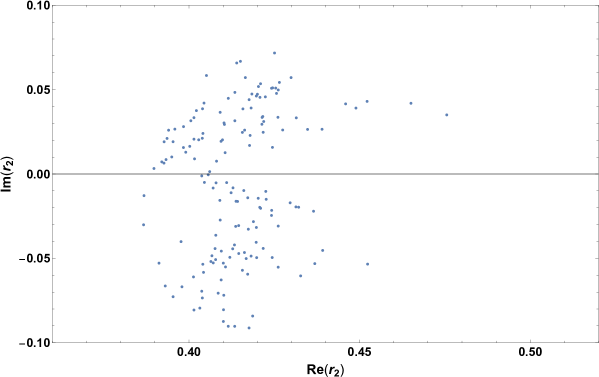
Figure 1: Distribution of $r_{2}$ (defined in Eq. (3)) in the fitting results satisfying the constraints of Table 2.

Now we plot the sets of values of $Y_{10},Y_{126},r_{1},r_{2},r_{L}$ satisfying Table 2, on the plane of $p\to K^{+}\bar{\nu}_{\mu}$ partial lifetime versus the ratio of the partial widths of $p\to K^{0}\mu^{+}$ and $p\to K^{+}\bar{\nu}_{\mu}$. From the plots, we read out the range of the partial width ratio predicted by the model.

We first study the contribution of individual terms in Eqs. (40)-(42) by taking $(a,b^{\prime},c^{\prime},d^{\prime})=(1,0,0,0),\,(0,1,0,0),\,(0,0,1,0),\,(0,0,0,1)$. The plots are in Fig. 2. We caution that although some points are apparently excluded by the current 90% CL experimental bound $1/\Gamma(p\to K^{+}\nu)>5.9\times 10^{33}$ years [55], these points are revived if $(a,b^{\prime},c^{\prime},d^{\prime})$ are reduced due to the mixing of (3, 1, $-\frac{1}{3}$), (${\bf\overline{3}}$, 1, $\frac{1}{3}$) components of fields other than $H,\overline{\Delta}$, or if SUSY particles are slightly heavier than the spectrum of Eq. (61) by factor $O(1)$.

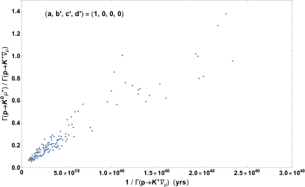
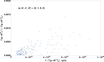
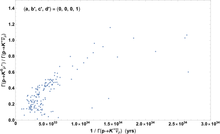
Figure 2: $p\to K^{+}\bar{\nu}_{\mu}$ partial lifetime versus the ratio of the partial widths of $p\to K^{0}\mu^{+}$ and $p\to K^{+}\bar{\nu}_{\mu}$. Each dot corresponds to a set of values of $Y_{10},Y_{126},r_{1},r_{2},r_{L}$ that satisfy the constraints of Table 2. We take $(a,b^{\prime},c^{\prime},d^{\prime})=(1,0,0,0),\,(0,1,0,0),\,(0,0,1,0),\,(0,0,0,1)$ in Eq. (40)-(42). Note that the vertical scale of the panel of $(a,b^{\prime},c^{\prime},d^{\prime})=(0,1,0,0)$ is different because the partial width ratio is quite suppressed in this case. Also, the horizontal scale is different for the four panels, due to the large hierarchy of $p\to K^{+}\bar{\nu}_{\mu}$ partial lifetime in the four cases. Although some points are apparently excluded by the current 90% CL experimental bound $1/\Gamma(p\to K^{+}\nu)>5.9\times 10^{33}$ years [55], these points are revived if $(a,b^{\prime},c^{\prime},d^{\prime})$ are reduced due to the mixing of (3, 1, $-\frac{1}{3}$), (${\bf\overline{3}}$, 1, $\frac{1}{3}$) components of fields other than $H,\overline{\Delta}$, or if SUSY particles are slightly heavier than the spectrum of Eq. (61).

We find that the predictions for $\Gamma(p\to K^{+}\bar{\nu}_{\mu})$ in the cases with $(a,b^{\prime},c^{\prime},d^{\prime})=(1,0,0,0)$, $(0,1,0,0)$, $(0,0,1,0)$, $(0,0,0,1)$ exhibit the following hierarchy:

$$({\rm case\ with\ }(1,0,0,0))\,\ll\,({\rm case\ with\ }(0,1,0,0))\,\lesssim\,({\rm case\ with\ }(0,0,1,0))\,\ll\,({\rm case\ with\ }(0,0,0,1))$$

On the other hand, the predictions for the partial width ratio $\Gamma(p\to K^{0}\mu^{+})/\Gamma(p\to K^{+}\bar{\nu}_{\mu})$ follow the following pattern:

$$({\rm case\ with\ }(0,1,0,0))\,\ll\,({\rm case\ with\ }(1,0,0,0))\,\sim\,({\rm case\ with\ }(0,0,1,0))\,\sim\,({\rm case\ with\ }(0,0,0,1))$$

From the above hierarchy patterns, we infer $\Gamma(p\to K^{0}\mu^{+})/\Gamma(p\to K^{+}\bar{\nu}_{\mu})$ for general values of $(a,b^{\prime},c^{\prime},d^{\prime})$ as follows.

• When $d^{\prime}=O(1)$, the partial width $\Gamma(p\to K^{+}\bar{\nu}_{\mu})$ is dominated by the contribution from the term with coefficient $d^{\prime}$. Since the partial width ratio $\Gamma(p\to K^{0}\mu^{+})/\Gamma(p\to K^{+}\bar{\nu}_{\mu})$ with $(a,b^{\prime},c^{\prime},d^{\prime})=(0,0,0,1)$ is comparable to or larger than in the other cases, we expect that $\Gamma(p\to K^{0}\mu^{+})$ is also dominated by the contribution from the term with $d^{\prime}$. Therefore, we conclude that when $d^{\prime}=O(1)$, irrespectively of the values of $a,b^{\prime},c^{\prime}$, the prediction on the partial width ratio is given by the lower-right panel of Fig. 2, where the partial width ratio mostly varies in the range 0.05-0.6. This result is consistent with our estimate Eq. (59).

• When $d^{\prime}=0$, the partial width $\Gamma(p\to K^{+}\bar{\nu}_{\mu})$ receives comparable contributions from the terms with $c^{\prime}$ and $b^{\prime}$. On the other hand, since the partial width ratio $\Gamma(p\to K^{0}\mu^{+})/\Gamma(p\to K^{+}\bar{\nu}_{\mu})$ with $(a,b^{\prime},c^{\prime},d^{\prime})=(0,1,0,0)$ is much smaller than that with $(a,b^{\prime},c^{\prime},d^{\prime})=(0,0,1,0)$, $\Gamma(p\to K^{0}\mu^{+})$ receives contribution solely from the term with $c^{\prime}$. Hence, when $c^{\prime}=O(1)$ and $b^{\prime}=O(1)$, the partial width ratio $\Gamma(p\to K^{0}\mu^{+})/\Gamma(p\to K^{+}\bar{\nu}_{\mu})$ is suppressed if the contributions of the terms with $c^{\prime}$ and $b^{\prime}$ to $\Gamma(p\to K^{+}\bar{\nu}_{\mu})$ interfere constructively, and the partial width ratio is enhanced if they interfere destructively. To examine these possibilities, we present plots for cases with $(a,b^{\prime},c^{\prime},d^{\prime})=(0,1,1,0)$, $(0,i,1,0)$, $(0,-1,1,0)$, $(0,-i,1,0)$ in Fig. 3.

  

  

  

  

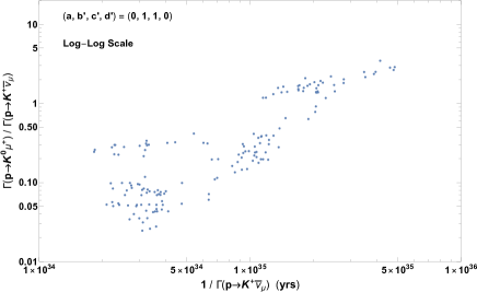
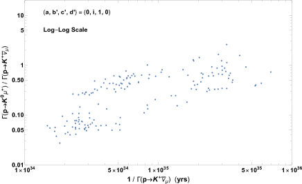
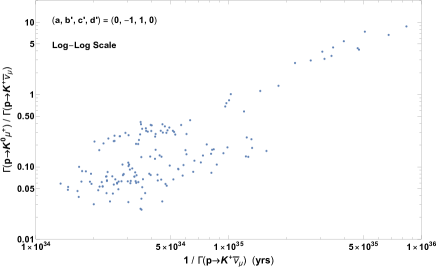
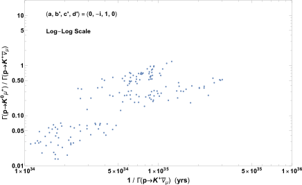
  Figure 3: Same as Fig. 2 except that we take $(a,b^{\prime},c^{\prime},d^{\prime})=(0,1,1,0)$, $(0,i,1,0)$, $(0,-1,1,0)$, $(0,-i,1,0)$ in Eq. (40)-(42).

  We observe that when $d^{\prime}=0$, $c^{\prime}=O(1)$ and $b^{\prime}=O(1)$, the prediction on the partial width ratio varies considerably with the relative phase of $b^{\prime}$ and $c^{\prime}$ and with different fitting results. Still, we can assert that the ratio is above 0.01. The absence of strong suppression factor $0.3\cdot 0.002$ is consistent with our estimate Eq. (59).

• When $d^{\prime}=b^{\prime}=0$, both $\Gamma(p\to K^{+}\bar{\nu}_{\mu})$ and $\Gamma(p\to K^{0}\mu^{+})$ are dominated by the contribution from the term with $c^{\prime}$. We thus conclude that when $d^{\prime}=b^{\prime}=0$, irrespectively of the value of $a$, the prediction on the partial width ratio is given by the lower-left panel of Fig. 2, where it varies in the ranges 0.03-0.2 and 0.4-0.8.

• When $d^{\prime}=c^{\prime}=0$, the partial width $\Gamma(p\to K^{+}\bar{\nu}_{\mu})$ is dominated by the contribution from the term with $b^{\prime}$. On the other hand, since the partial width ratio $\Gamma(p\to K^{0}\mu^{+})/\Gamma(p\to K^{+}\bar{\nu}_{\mu})$ is much larger with $(a,b^{\prime},c^{\prime},d^{\prime})=(1,0,0,0)$ than with $(a,b^{\prime},c^{\prime},d^{\prime})=(0,1,0,0)$, $\Gamma(p\to K^{0}\mu^{+})$ might receive larger contribution from the term with $a$ than from the term with $b^{\prime}$. However, we have inspected cases with $(a,b^{\prime},c^{\prime},d^{\prime})=(1,1,0,0)$, $(i,1,0,0)$, $(-1,1,0,0)$, $(-i,1,0,0)$ and found that the distribution in these cases is almost identical to that with $(a,b^{\prime},c^{\prime},d^{\prime})=(0,1,0,0)$. We thus conclude that when $d^{\prime}=c^{\prime}=0$, irrespectively of the value of $a$, the prediction on the partial width ratio is given by the upper-right panel of Fig. 2, where it is mostly suppressed below 0.0005. This result agrees with our estimate Eq. (60).

• Only in the very special case with $d^{\prime}=c^{\prime}=b^{\prime}=0$ do we obtain the distribution of the upper-left panel of Fig. 2, where the ratio is above 0.05.

To summarize, if $d^{\prime}=O(1)$, the partial width ratio $\Gamma(p\to K^{0}\mu^{+})/\Gamma(p\to K^{+}\bar{\nu}_{\mu})$ is mostly in the range 0.05-0.6. If $d^{\prime}=0$, $c^{\prime}=O(1)$ and $b^{\prime}=O(1)$, the partial width ratio varies in a wide range, still it is above 0.01. If $d^{\prime}=b^{\prime}=0$ and $c^{\prime}=O(1)$, it is in the ranges 0.03-0.2 and 0.4-0.8. If $d^{\prime}=c^{\prime}=b^{\prime}=0$, it is above 0.05. Only when $d^{\prime}=c^{\prime}=0$ and $b^{\prime}=O(1)$ is the partial width ratio mostly highly suppressed below 0.0005.

Because there is no particular reason to believe $d^{\prime}=0$, our most important result is the lower-right panel of Fig. 2, which covers the case with $d^{\prime}=O(1)$. Accordingly, our main prediction is

$$0.6\ \gtrsim\ \frac{\Gamma(p\to K^{0}\mu^{+})}{\Gamma(p\to K^{+}\bar{\nu}_{\mu})}\ \gtrsim\ 0.05.$$ (68)

Considering the current 90% CL bound $1/\Gamma(p\to K^{+}\nu)>5.9\times 10^{33}$ years [55], we can at best observe the $p\to K^{0}\mu^{+}$ decay at a rate $1/\Gamma(p\to K^{0}\mu^{+})=1\times 10^{34}$ years.

5 Summary

The ratio of the partial widths of some dimension-5 proton decay modes can be predicted without knowledge of SUSY particle masses, and thus serves as a probe for various SUSY GUT models even when SUSY particles are not discovered. We have focused on the partial width ratio $\Gamma(p\to K^{0}\mu^{+})/\Gamma(p\to K^{+}\bar{\nu}_{\mu})$ in the minimal renormalizable SUSY $SO(10)$ GUT. In the model, the Wilson coefficients of dimension-5 operators responsible for the $p\to K^{0}\mu^{+}$ and the $p\to K^{+}\bar{\nu}_{\mu}$ decays are on the same order, and $\Gamma(p\to K^{0}\mu^{+})/\Gamma(p\to K^{+}\bar{\nu}_{\mu})$ is largely determined by the ratio of baryon chiral Lagrangian parameters and is estimated to be $O(0.1)$. This is in striking contrast to the minimal $SU(5)$ GUT, where this partial width ratio is further suppressed by factor $y_{u}^{2}/(\lambda^{2}y_{c})^{2}\simeq 0.002$. To confirm that $\Gamma(p\to K^{0}\mu^{+})/\Gamma(p\to K^{+}\bar{\nu}_{\mu})=O(0.1)$ in the minimal renormalizable SUSY $SO(10)$ GUT, we have numerically determined $Y_{10},Y_{126}$ through a fitting of the quark and charged lepton Yukawa couplings and neutrino mass matrix, and calculated the partial width ratio based on the fitting results. Our most important finding is that the partial width ratio generally varies in the range $0.6\gtrsim\Gamma(p\to K^{0}\mu^{+})/\Gamma(p\to K^{+}\bar{\nu}_{\mu})\gtrsim 0.05$ in the most generic case where $d^{\prime}=O(1)$ in Eqs. (40)-(42).

References

- [1] H. Georgi, “The State of the Art—Gauge Theories,” AIP Conf. Proc. 23, 575 (1975).
- [2] H. Fritzsch and P. Minkowski, “Unified Interactions of Leptons and Hadrons,” Annals Phys. 93, 193 (1975).
- [3] P. Minkowski, “ at a Rate of One Out of Muon Decays?,” Phys. Lett. 67B, 421 (1977).
- [4] T. Yanagida, “Horizontal Symmetry And Masses Of Neutrinos,” Conf. Proc. C 7902131, 95 (1979).
- [5] S. L. Glashow, “The Future of Elementary Particle Physics,” NATO Sci. Ser. B 61, 687 (1980).
- [6] R. N. Mohapatra and G. Senjanovic, “Neutrino Mass and Spontaneous Parity Violation,” Phys. Rev. Lett. 44, 912 (1980).
- [7] K. S. Babu and R. N. Mohapatra, “Predictive neutrino spectrum in minimal SO(10) grand unification,” Phys. Rev. Lett. 70, 2845 (1993) [hep-ph/9209215].
- [8] S. Weinberg, “Supersymmetry at Ordinary Energies. 1. Masses and Conservation Laws,” Phys. Rev. D 26, 287 (1982).
- [9] N. Sakai and T. Yanagida, “Proton Decay in a Class of Supersymmetric Grand Unified Models,” Nucl. Phys. B 197, 533 (1982).
- [10] K. Abe et al. [Hyper-Kamiokande Collaboration], “Hyper-Kamiokande Design Report,” arXiv:1805.04163 [physics.ins-det].
- [11] N. Haba, Y. Mimura and T. Yamada, “Detectable dimension-6 proton decay in SUSY SO(10) GUT at Hyper-Kamiokande,” JHEP 1907, 155 (2019) [arXiv:1904.11697 [hep-ph]].
- [12] K. Matsuda, Y. Koide and T. Fukuyama, “Can the SO(10) model with two Higgs doublets reproduce the observed fermion masses?,” Phys. Rev. D 64, 053015 (2001) [hep-ph/0010026].
- [13] K. Matsuda, Y. Koide, T. Fukuyama and H. Nishiura, “How far can the SO(10) two Higgs model describe the observed neutrino masses and mixings?,” Phys. Rev. D 65, 033008 (2002) Erratum: [Phys. Rev. D 65, 079904 (2002)] [hep-ph/0108202].
- [14] T. Fukuyama and N. Okada, “Neutrino oscillation data versus minimal supersymmetric SO(10) model,” JHEP 0211, 011 (2002) [hep-ph/0205066].
- [15] B. Bajc, G. Senjanovic and F. Vissani, “b - tau unification and large atmospheric mixing: A Case for noncanonical seesaw,” Phys. Rev. Lett. 90, 051802 (2003) [hep-ph/0210207].
- [16] B. Bajc, G. Senjanovic and F. Vissani, “Probing the nature of the seesaw in renormalizable SO(10),” Phys. Rev. D 70, 093002 (2004) [hep-ph/0402140].
- [17] H. S. Goh, R. N. Mohapatra and S. P. Ng, “Minimal SUSY SO(10), b tau unification and large neutrino mixings,” Phys. Lett. B 570, 215 (2003) [hep-ph/0303055].
- [18] C. S. Aulakh, B. Bajc, A. Melfo, G. Senjanovic and F. Vissani, “The Minimal supersymmetric grand unified theory,” Phys. Lett. B 588, 196 (2004) [hep-ph/0306242].
- [19] H. S. Goh, R. N. Mohapatra and S. P. Ng, “Minimal SUSY SO(10) model and predictions for neutrino mixings and leptonic CP violation,” Phys. Rev. D 68, 115008 (2003) [hep-ph/0308197].
- [20] B. Dutta, Y. Mimura and R. N. Mohapatra, “CKM CP violation in a minimal SO(10) model for neutrinos and its implications,” Phys. Rev. D 69, 115014 (2004) [hep-ph/0402113].
- [21] B. Dutta, Y. Mimura and R. N. Mohapatra, “Neutrino masses and mixings in a predictive SO(10) model with CKM CP violation,” Phys. Lett. B 603, 35 (2004) [hep-ph/0406262].
- [22] K. S. Babu and C. Macesanu, “Neutrino masses and mixings in a minimal SO(10) model,” Phys. Rev. D 72, 115003 (2005) [hep-ph/0505200].
- [23] S. Bertolini, T. Schwetz and M. Malinsky, “Fermion masses and mixings in SO(10) models and the neutrino challenge to SUSY GUTs,” Phys. Rev. D 73, 115012 (2006) [hep-ph/0605006].
- [24] A. S. Joshipura and K. M. Patel, “Fermion Masses in SO(10) Models,” Phys. Rev. D 83, 095002 (2011) [arXiv:1102.5148 [hep-ph]].
- [25] A. Dueck and W. Rodejohann, “Fits to SO(10) Grand Unified Models,” JHEP 1309, 024 (2013) [arXiv:1306.4468 [hep-ph]].
- [26] T. Fukuyama, K. Ichikawa and Y. Mimura, “Revisiting fermion mass and mixing fits in the minimal SUSY GUT,” Phys. Rev. D 94, no. 7, 075018 (2016) [arXiv:1508.07078 [hep-ph]].
- [27] T. Fukuyama, K. Ichikawa and Y. Mimura, “Relation between proton decay and PMNS phase in the minimal SUSY GUT,” Phys. Lett. B 764, 114 (2017) [arXiv:1609.08640 [hep-ph]].
- [28] T. Fukuyama, N. Okada and H. M. Tran, “Sparticle spectroscopy of the minimal SO(10) model,” Phys. Lett. B 767, 295 (2017) [arXiv:1611.08341 [hep-ph]].
- [29] K. S. Babu, B. Bajc and S. Saad, “Resurrecting Minimal Yukawa Sector of SUSY SO(10),” JHEP 1810, 135 (2018) [arXiv:1805.10631 [hep-ph]].
- [30] T. Deppisch, S. Schacht and M. Spinrath, “Confronting SUSY SO(10) with updated Lattice and Neutrino Data,” JHEP 1901, 005 (2019) [arXiv:1811.02895 [hep-ph]].
- [31] K. S. Babu, J. C. Pati and F. Wilczek, “Suggested new modes in supersymmetric proton decay,” Phys. Lett. B 423, 337 (1998) [hep-ph/9712307].
- [32] K. S. Babu, J. C. Pati and F. Wilczek, “Fermion masses, neutrino oscillations, and proton decay in the light of Super-Kamiokande,” Nucl. Phys. B 566, 33 (2000) [hep-ph/9812538].
- [33] T. Fukuyama, A. Ilakovac, T. Kikuchi, S. Meljanac and N. Okada, “General formulation for proton decay rate in minimal supersymmetric SO(10) GUT,” Eur. Phys. J. C 42, 191 (2005) [hep-ph/0401213].
- [34] C. S. Aulakh and A. Girdhar, “SO(10) MSGUT: Spectra, couplings and threshold effects,” Nucl. Phys. B 711, 275 (2005) [hep-ph/0405074].
- [35] T. Fukuyama, A. Ilakovac, T. Kikuchi, S. Meljanac and N. Okada, “SO(10) group theory for the unified model building,” J. Math. Phys. 46, 033505 (2005) [hep-ph/0405300].
- [36] T. Fukuyama, A. Ilakovac, T. Kikuchi, S. Meljanac and N. Okada, “Higgs masses in the minimal SUSY SO(10) GUT,” Phys. Rev. D 72, 051701 (2005) [hep-ph/0412348].
- [37] B. Bajc, A. Melfo, G. Senjanovic and F. Vissani, “The Minimal supersymmetric grand unified theory. 1. Symmetry breaking and the particle spectrum,” Phys. Rev. D 70, 035007 (2004) [hep-ph/0402122].
- [38] B. Bajc, A. Melfo, G. Senjanovic and F. Vissani, “Fermion mass relations in a supersymmetric SO(10) theory,” Phys. Lett. B 634, 272 (2006) [hep-ph/0511352].
- [39] J. Hisano, H. Murayama and T. Yanagida, “Nucleon decay in the minimal supersymmetric SU(5) grand unification,” Nucl. Phys. B 402, 46 (1993) [hep-ph/9207279].
- [40] T. Goto and T. Nihei, “Effect of RRRR dimension five operator on the proton decay in the minimal SU(5) SUGRA GUT model,” Phys. Rev. D 59, 115009 (1999) [hep-ph/9808255].
- [41] A. Bazavov et al. [MILC Collaboration], “MILC results for light pseudoscalars,” PoS CD 09, 007 (2009) [arXiv:0910.2966 [hep-ph]].
- [42] S. Durr et al., “Lattice QCD at the physical point: light quark masses,” Phys. Lett. B 701, 265 (2011) [arXiv:1011.2403 [hep-lat]].
- [43] S. Durr et al., “Lattice QCD at the physical point: Simulation and analysis details,” JHEP 1108, 148 (2011) [arXiv:1011.2711 [hep-lat]].
- [44] C. McNeile, C. T. H. Davies, E. Follana, K. Hornbostel and G. P. Lepage, “High-Precision c and b Masses, and QCD Coupling from Current-Current Correlators in Lattice and Continuum QCD,” Phys. Rev. D 82, 034512 (2010) [arXiv:1004.4285 [hep-lat]].
- [45] T. Blum et al. [RBC and UKQCD Collaborations], “Domain wall QCD with physical quark masses,” Phys. Rev. D 93, no. 7, 074505 (2016) [arXiv:1411.7017 [hep-lat]].
- [46] A. Bazavov et al., “Staggered chiral perturbation theory in the two-flavor case and SU(2) analysis of the MILC data,” PoS LATTICE 2010, 083 (2010) [arXiv:1011.1792 [hep-lat]].
- [47] S. Aoki et al., “Review of lattice results concerning low-energy particle physics,” Eur. Phys. J. C 77, no. 2, 112 (2017) [arXiv:1607.00299 [hep-lat]].
- [48] K. G. Chetyrkin, J. H. Kuhn, A. Maier, P. Maierhofer, P. Marquard, M. Steinhauser and C. Sturm, Phys. Rev. D 80, 074010 (2009) doi:10.1103/PhysRevD.80.074010 [arXiv:0907.2110 [hep-ph]].
- [49] G. Aad et al. [ATLAS Collaboration], “Measurement of the top-quark mass in -jet events collected with the ATLAS detector in collisions at TeV,” arXiv:1905.02302 [hep-ex].
- [50] J. Charles et al. [CKMfitter Group], “CP violation and the CKM matrix: Assessing the impact of the asymmetric factories,” Eur. Phys. J. C 41, no. 1, 1 (2005) [hep-ph/0406184], updated results and plots available at: http://ckmfitter.in2p3.fr
- [51] M. Tanabashi et al. [Particle Data Group], “Review of Particle Physics,” Phys. Rev. D 98, no. 3, 030001 (2018).
- [52] I. Esteban, M. C. Gonzalez-Garcia, A. Hernandez-Cabezudo, M. Maltoni and T. Schwetz, “Global analysis of three-flavour neutrino oscillations: synergies and tensions in the determination of , , and the mass ordering,” JHEP 1901, 106 (2019) [arXiv:1811.05487 [hep-ph]].
- [53] I. Esteban, M. C. Gonzalez-Garcia, A. Hernandez-Cabezudo, M. Maltoni and T. Schwetz, NuFIT 4.1 (2019), www.nu-fit.org.
- [54] Y. Aoki, T. Izubuchi, E. Shintani and A. Soni, “Improved lattice computation of proton decay matrix elements,” Phys. Rev. D 96, no. 1, 014506 (2017) [arXiv:1705.01338 [hep-lat]].
- [55] K. Abe et al. [Super-Kamiokande Collaboration], “Search for proton decay via using 260 kiloton*year data of Super-Kamiokande,” Phys. Rev. D 90, no. 7, 072005 (2014) [arXiv:1408.1195 [hep-ex]].