Disentangling Image Distortions in Deep Feature Space

Abstract

Previous literature suggests that perceptual similarity is an emergent property shared across deep visual representations. Experiments conducted on a dataset of human-judged image distortions have proven that deep features outperform classic perceptual metrics. In this work we take a further step in the direction of a broader understanding of such property by analyzing the capability of deep visual representations to intrinsically characterize different types of image distortions. To this end, we firstly generate a number of synthetically distorted images and then we analyze the features extracted by different layers of different Deep Neural Networks. We observe that a dimension-reduced representation of the features extracted from a given layer permits to efficiently separate types of distortions in the feature space. Moreover, each network layer exhibits a different ability to separate between different types of distortions, and this ability varies according to the network architecture. Finally, we evaluate the exploitation of features taken from the layer that better separates image distortions for: i) reduced-reference image quality assessment, and ii) distortion types and severity levels characterization on both single and multiple distortion databases. Results achieved on both tasks suggest that deep visual representations can be unsupervisedly employed to efficiently characterize various image distortions.

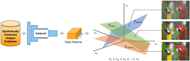
Fig. 1: Are deep features intrinsically able to characterize image distortions? The deep features extracted from a specific layer of a network trained for a recognition task, intrinsically divide the deep feature space in such a way that visual representations corresponding to different types of distortions lay on different planes.

1 Motivation

The networks trained to discriminate a wide variety of categories contained within the images allow to obtain rich representations that can be reused for other tasks in which it is necessary to carry out a semantic analysis of the image. Deep features extracted from common networks trained for recognition tasks, such as ImageNet challenge Russakovsky et al. (2015), have been demonstrated to be very effective for transfer learning in many tasks Sharif Razavian et al. (2014). Moreover, what makes pretrained networks good for transfer learning is not directly connected to the amount of data but probably to the network architecture itself Huh et al. (2016). Literature has also highlighted another surprising property of pretrained networks: visual deep representation can be adopted as metric for perceptual similarity. This property was firstly experienced for feature inversion Mahendran and Vedaldi (2015), feature visualization Simonyan et al. (2013); Yosinski et al. (2015), texture synthesis and style transfer Gatys et al. (2015a, b). The most remarkable paper in this direction demonstrates that high-level features from a pretrained network on ImageNet can be efficiently employed as a perceptual loss to train feed-forward transformation networks for image transformation tasks Johnson et al. (2016). A recent paper Zhang et al. (2018) tried to answer to the following questions: i) “how perceptual are these so-called perceptual losses?”; ii) “what elements are critical for their success?”. The findings of this paper suggest that perceptual similarity is an emergent property shared across deep visual representations that outperform, by a large margin, classic perceptual metrics such as SSIM Wang et al. (2004) for image distortion characterization. This property has been assessed on a large-scale highly diverse dataset of perceptual judgments specially collected for this scope. The dataset included images with different kinds of image distortions: traditional, obtained by performing basic low-level image editing operations; CNN-based distortions, obtained by randomly varying parameters, etc. Although the paper provides a comprehensive demonstration that deep features catch perceptual properties of the images better than traditional metrics, further understanding should be provided in the direction of explaining how deep features characterize image distortions.

We want here to go one step further. What we would really like to understand is: are deep networks able to effectively characterize image distortions? If so, is this capability different on the basis of network architectures? Which layer provides the representation better disentangling distortions? Can dimensional reduction techniques help to strengthen this property? In this paper, we conduct a comprehensive study of deep features extracted across different networks and compare them in terms of distortions separability indices. This is motivated by the fact that we assume that deep features representing images affected by the same type of distortions should be similar and so they might form clusters. We find that deep features are able to intrinsically disentangle image distortions and that this property is not equally revealed across networks and layers.

The main contributions of this paper are as follows:

• We conduct a comprehensive analysis of deep features for several networks in order to understand which one is the most effective for image distortion characterization.

• We show that deep features obtaining a high distortion separability index can obtain comparable results with respect to reduced-reference image quality assessment methods on four widely used benchmark databases for the distortion characterization task.

• We demonstrate that the evaluated property might be exploited for the recognition of image distortion types and severity levels on single and multiple distortion databases.

2 Data

To evaluate how visual features deal with different types and severity of image distortions, we create our own database, that differently from available ones, has a larger and controlled number of severity levels. In particular, we generate 783 synthetically distorted images by applying three mainstream distortion types to the 29 reference images of the LIVE database Sheikh (2005): additive white Gaussian noise (AWGN), Gaussian blur (GBlur), and JPEG compression (JPEG). More in detail, each reference image is corrupted by applying each one of the following operations:

• AWGN: The noise is generated from a standard normal distribution of zero mean and standard deviation $\sigma_{N}$ and then added to each color channel;

• GBlur: A Gaussian kernel with standard deviation $\sigma_{G}$ is applied for blurring with a square kernel window each of the three planes using the function gaussian_filter of the Scipy.ndimage Virtanen et al. (2019) package;

• JPEG: JPEG compressed images are obtained by varying the quality parameter ($Q$) of save function of the Pillow library(whose range is from 1 to 100, with 100 representing the best quality), which indicates the degree of the JPEG compression algorithm.

For each type of image distortion we consider the following values which cause several levels of severity:

$\sigma_{N}=(0.03,0.06,0.09,0.13,0.18,0.24,0.31,0.50,1.89)$,
$\sigma_{G}=(0.62,0.82,0.95,1.13,1.42,1.65,2.17,3.54,13.00)$,
$Q=(80,60,45,30,20,15,10,5,2)$.

Values are chosen in such a way that distorted images are perceptually separable from each other. Each type and severity level of image distortions are applied to each reference image. Figure 2 shows for a given reference image the corresponding synthetically generated distorted images.

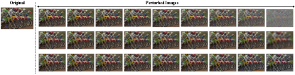
Fig. 2: Samples from the generated database. The original image and corresponding perturbed versions with increasing distortion severity from the left to the right. First row shows images affected by additive white Gaussian noise (AWGN), the second row contains images corrupted by Gaussian blur (GBlur), finally the last row reports images with different JPEG compression levels (JPEG).

3 Disentangling Image Distortions

The intuition here is that a visual deep feature space, suitably defined, permits to efficiently disentangle image distortion types. To pursue this idea, we firstly build a deep feature space by aggregating features extracted from a single layer of a network. Secondly, we evaluate how much such a space effectively permits to separate among the three types of distortions by computing separability indices of the feature space. Figure 3 illustrates the entire pipeline for disentangling image distortions. To evaluate how much this property of the feature space depends on the architecture of the network, we evaluate several architectures.

Network architectures

We consider the AlexNet Krizhevsky et al. (2012), Inception-v3 Szegedy et al. (2016), ResNet-50 He et al. (2016), SqueezeNet-v1.1 Iandola et al. (2016), and VGG-16 Simonyan and Zisserman (2014) architectures. We use the conv1-conv5 layers from AlexNet, which is a popular deep CNN model widely applied in computer vision and includes computations that are loosely matched to the human visual cortex, such as pooling and local response normalization. We extract features from the three convolution layers, namely 2a3x3, 3b1x1, 4a3x3, and all the inception layers (called mixed) of the Inception-v3 network, which introduced the use of factorized convolutions by using asymmetric convolutions. For ResNet-50, we extract features for conv1 and subsequent macro-residual blocks (named layer). We evaluate the SqueezeNet-v1.1 architecture by using the first conv1 layer and all the fire layers activations. Finally, we take the conv layers of VGG-16, which is usually used as a perceptual metric in image generation.

Deep Feature Space

Given a network level $l$, producing a deep feature block of size $h_{l}\times w_{l}\times c_{l}$, and an image taken from the synthetically distorted dataset, we calculate a deep visual representation by averaging features across spatial dimensions, thus obtaining a vector of size $1\times c_{l}$ (see Fig. 3). The images are used at their original sizes so as not to mask artifacts.

Data separation

All the $1\times c_{l}$ vectors extracted from all the images of the synthetically distorted dataset are grouped by relying on the three types of distortions: AWGN, GBlur and JPEG. Goodness of the resulting clusters is then evaluated using several separability metrics.

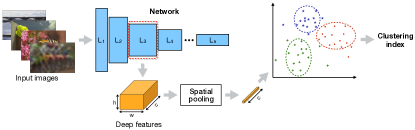
Fig. 3: Clusters evaluation. Each full-size image of the generated database is fed into a network, the deep features are obtained by using the activations of a specific layer, so the average spatial pooling is applied and finally, we measure the quality of the clusters that group the images affected by the same type of distortion.

4 Cluster separability indices

To evaluate the quality of the clusters that are formed using the deep features computed for images affected by different types and levels of distortions, we consider a combination of three internal cluster validity indices Arbelaitz et al. (2013); van Craenendonck and Blockeel (2015), which rely only on properties intrinsic of the structure of clusters and their relations to each other, namely: the Calinski-Harabasz index Caliński and Harabasz (1974), the Davies-Bouldin index Davies and Bouldin (1979), and the Silhouette index Rousseeuw (1987).

Calinski-Harabasz index

The Calinski-Harabasz (CH) index Caliński and Harabasz (1974), also known as Variance Ratio Criterion, estimates the clusters goodness in terms of ratio between the between-clusters variance ($SS_{B}$) and the within-clusters variance ($SS_{W}$). It is defined as follows:

$$CH=\frac{SS_{B}}{SS_{W}}\times\frac{N-K}{K-1},$$ (1)

where $N$ is the number of samples, and $K=3$ represents the number of clusters (which are AWGN, GBlur and JPEG). $SS_{W}$ is specified as $SS_{W}=\sum_{k=1}^{K}{\sum_{x\in C_{k}}{\left\lVert x-G_{k}\right\rVert^{2}}}$, given $C_{k}$ the set of samples in the cluster $k$, and $G_{k}$ the center of the cluster $k$. Finally, $SS_{B}=\sum_{k=1}^{K}{n_{k}\left\lVert G_{k}-G\right\rVert^{2}}$, where $n_{k}$ is the number of points in the cluster $k$, and $G$ is the center of the whole dataset. The score is higher when elements from the same clusters are quite close and clusters itself are well separated.

Davies-Bouldin index

The Davies-Bouldin (DB) index Davies and Bouldin (1979) measures the average similarity between clusters and is based on the dispersion measure of a cluster ($\delta_{k}$) and the cluster dissimilarity measure ($\Delta_{kk^{\prime}}$). The dispersion measure is the mean distance of the points belonging to cluster $C_{k}$ to their center $G_{k}$, $\delta_{k}=\frac{1}{n_{k}}\sum_{x\in C_{k}}{\left\lVert x-G_{k}\right\rVert}$, while $\Delta_{kk^{\prime}}=\left\lVert G_{k^{\prime}}-G_{k}\right\rVert$ is the distance between the centroids $G_{k^{\prime}}$ and $G_{k}$ of clusters $C_{k^{\prime}}$ and $C_{k}$. The DB is then defined as:

$$\qquad DB=\frac{1}{K}\sum^{K}_{k=1}{\max_{k^{\prime}\neq k}\left(\frac{\delta_{k}+\delta_{k^{\prime}}}{\Delta_{kk^{\prime}}}\right)}.$$ (2)

Zero is the lowest possible score, values closer to zero indicate a better separation between data.

Silhouette index

The Silhouette index (S) Rousseeuw (1987) is defined as the mean of the silhouette widths for each sample and is formalized as follows:

$$S=\frac{1}{K}\sum_{k=1}^{K}{\frac{1}{n_{k}}\sum_{x\in C_{k}}{s(x)}},$$ (3)

where the silhouette width $s(x)$ for each sample is computed as $s(x)=\frac{b(x)-a(x)}{\max(a(x),b(x))}$. $a(x)$ is the mean distance between the sample $x$, such that $x\in C_{k}$, and the set of samples in the cluster it belongs to, $C_{k}$. $b(x)$ represents the mean dissimilarity of a sample $x$ with respect to the nearest cluster, namely $b(x)=\min_{k^{\prime}\neq k}\frac{1}{n_{k^{\prime}}}\sum_{y\in C_{k^{\prime}}}{d(x,y)}$. Higher values of the silhouette index denotes a better quality of clusters.

Combination of separability indices

To understand which layer of a network provides a better separation of clusters we combine the previous indices into a single one as follows: first, we individually perform a min-max normalization in the range [0,1] of the scores obtained for each index by taking the maximum and minimum values for that index over all the layers $l\in L$ of all the network architectures $n\in N$ considered:

$$x^{\prime}(l)=\frac{x(l)-\min\limits_{l\in L,n\in N}x(l_{n})}{\max\limits_{l\in L,n\in N}x(l_{n})-\min\limits_{l\in L,n\in N}x(l_{n})}$$ (4)

with $x=\left\{CH,DB,S\right\}$. Then we estimate the overall distortions separability index $DSI(l)$ for each network layer $l$ in this way:

$$DSI(l)=\frac{1}{3}\left[CH^{\prime}(l)+\left(1-DB^{\prime}(l)\right)+S^{\prime}(l)\right]$$ (5)

The resulting $DSI(l)$ score ranges between 0 and 1 and the higher is the value the better is the separability of the clusters.

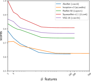
Fig. 4: Distortions separability indices obtained by varying the number of features in deep feature vectors using principal component analysis (PCA) for the layer achieving the best distortions separability index of each network considered.

5 Analysis

In this section we describe the experiments we conducted to verify the effectiveness of deep features for image distortion characterization. We implement our experiments using the PyTorch framework Paszke et al. (2017) and by exploiting the pretrained networks on ImageNet contained in the Torchvision package.

Are the deep features extracted from different networks equally capable of characterizing the various types of distortions? Are all the layers of the network equally effective to characterize distortions?

Table 1 reports the distortions separability index $DSI(l)$ achieved on each layer $l$ of the different networks, pretrained on Imagenet, we considered. Low scores (in red) denote that clusters can not be well separated, while high scores (in green) denote the opposite. The resulting rank of layers per network indicates that the deep features extracted from the first layer get almost always the worst position. We obtain that the layer for each network achieving the best clustering index is the following: conv2 for AlexNet, mixed6a of the Inception-v3 network, layer1 in ResNet-50, the layer fire4 of SqueezeNet-v1.1, and conv31 for the VGG-16 network. Among all the best layers, the fire4 layer of SqueezeNet-v1.1 is the best. Previous results confirm our intuition that some visual representations corresponding to different types of distortions distribute in well-separated regions of the deep feature space.

Does dimensionality reduction of deep features improve image distortion characterization?

Figure 4 shows the distortions separability index obtained by varying the number of features thanks to the use of principal component analysis (PCA) Wold et al. (1987). For each network, we consider the index for the layer that attained the best score in the previous analysis. We can see that by reducing the dimensionality of the features, the distortions separability index increases for all the networks and more in detail it reaches the peak value for 2-dimensional feature vectors. The only network showing a different trend, i.e. lower distortions separability index for bidimensional vectors, is Inception-v3.

Does the capability of discriminating distortions belong to the network architecture or it depends on the network weights?

In this experiment images are encoded by using deep features extracted from randomly initialized networks. For statistical significance we compute the final distortions separability index for each layer by averaging the scores obtained for 100 network re-initializations. Resulting scores for each layer are definitely lower than the ones obtained in the previous experiment indicating that the degree of separability of images affected by diverse distortions is limited. The ranks of layers per network are completely different from the ones obtained in the previous experiment, but given that the standard deviation of distortions separability indices among layers is small, we can not consider this aspect significant.

Can the removal of semantics from the visual representation of the image emphasize the distortion encoding?

In this experiment we want to understand if the separability property of clusters in the deep feature space is influenced by the content of the images. For doing that, we subtract in channel dimension the vector of features, of size $1\times c_{l}$, of the reference image to the feature vector of the distorted image. The results of this experiment indicate that the semantics does not affect the rank of the layers for AlexNet, VGG-16, as well as for ResNet-50 which, however, presents an increase in the distortions separability index for the best layer. This may be due to the presence of skip connections that carry low-level information from previous layers. Both Inception-v3 and SqueezeNet-v1.1 obtain a different rank of layers with also lower scores for the distortions separability index.

Table 1: Distortions separability indices for each layer of the considered networks pretrained on ImageNet. The indices are calculated by combining three internal cluster validity indices and are included in the interval [0,1], in which the highest scores (in green) indicate a high separability of the types of distortions, while the low scores (in red) represent levels not able to separate the clusters that are formed to discriminate the different distortions.

Network	Layer
AlexNet	conv1	conv2	conv3	conv4	conv5
	0.5748	0.6214	0.5614	0.5108	0.4978
Inception-v3	2a3x3	3b1x1	4a3x3	mixed5b	mixed5c	mixed5d	mixed6a	mixed6b	mixed6c	mixed6d	mixed6e	mixed7a	mixed7b	mixed7c
	0.4387	0.5284	0.5652	0.5979	0.6052	0.6347	0.6641	0.6254	0.6264	0.5867	0.5388	0.5348	0.5412	0.5564
ResNet-50	conv1	layer1	layer2	layer3	layer4
	0.4551	0.7268	0.5930	0.4615	0.4615
SqueezeNet-v1.1	conv1	fire1	fire2	fire3	fire4	fire5	fire6	fire7	fire8
	0.5186	0.7002	0.7535	0.7567	0.8081	0.7583	0.6863	0.6174	0.7433
VGG-16	conv11	conv12	conv21	conv22	conv31	conv32	conv33	conv41	conv42	conv43	conv51	conv52	conv53
	0.5190	0.6650	0.7408	0.7634	0.7678	0.7559	0.6153	0.5830	0.5651	0.5218	0.4879	0.4506	0.4327

6 Applications

We demonstrate usefulness of the investigated property by experimenting on two quality assessment tasks, namely: reduced-reference image quality assessment (RR-IQA) on four public databases and distortion recognition on single and multiple distortion databases.

6.1 Reduced-Reference Image Quality Assessment

We conduct experiments on the reduced-reference image quality assessment (RR-IQA) task Wang and Bovik (2006, 2011) in which we do not try to estimate the exact quality score but we verify that the rank between the images with different distortions is respected. First we encode both the distorted image and its reference one by using the activations of the layers we demonstrated achieve the best distortions separability index, i.e. layers of pretrained networks on ImageNet. Then we measure the pairwise Euclidean distance between the feature vectors of the distorted image and its reference image, and finally we estimate the correlation between this distance and the database ground-truth. We evaluate the method on four common image databases, which are LIVE Sheikh (2005), CSIQ Larson and Chandler (2010), TID2008 Ponomarenko et al. (2009), TID2013 Ponomarenko et al. (2013). Information about these four databases is summarized in Table 2.

Table 2: Description of the four image quality databases used for the reduced-reference image quality assessment.

Databases	Reference images	Distorted images	Distortion types	Distortion levels
CSIQ Larson and Chandler (2010)	30	886	6	4-5
LIVE Sheikh (2005)	29	779	5	7-8
TID2008 Ponomarenko et al. (2009)	25	1,700	17	4
TID2013 Ponomarenko et al. (2013)	25	3,000	24	5

Table 3 reports the median and the mean SROCC and PLCC for each database and network considered. The fire4 layer of the SqueezeNet-v1.1 network provides deep visual representations correlating well with human observers for CSIQ and LIVE databases. Instead, for both the TID2008 and TID2013 databases the conv2 layer of AlexNet is the one achieving the highest correlation values.

Table 4 compares state of the art methods with our best solutions on each one of the three types of distortions we considered. First of all, we want to highlight that even without any training, the performance of our solutions attains comparable results with respect to methods explicitly developed to face the image quality assessment task. In particular, the average SROCC across all distortions and datasets ranks S4RR Zhang et al. (2017) as the best method with an average correlation of 0.9549, followed by our proposed method using AlexNet with an average correlation of 0.9238.

Moreover, considering each distortion type separately, on AWGN the proposed method with AlexNet obtains the highest average SROCC equal to 0.9550 followed by S4RR with an average SROCC of 0.9522; on JPEG S4RR obtains the highest average SROCC of 0.9563, while the proposed method with AlexNet obtains the second highest average SROCC of 0.9435; on GBlur instead S4RR obtains the highest average correlation of 0.9563, with SSIM obtaining the second highest correlation of 0.9238.

Table 3: Median and mean SROCC and PLCC values across 100 train-test random splits on CSIQ, LIVE, TID2008, and TID2013 databases for the considered networks.

Database	Network	Median		Mean
		SROCC	PLCC	SROCC	PLCC
CSIQ	AlexNet	0.9300	0.9050	0.9284	0.9003
	Inception-v3	0.9120	0.9106	0.9105	0.9081
	ResNet-50	0.9228	0.9146	0.9225	0.9111
	SqueezeNet-v1.1	0.9301	0.9072	0.9300	0.9055
	VGG-16	0.8898	0.8547	0.8793	0.8394
LIVE	AlexNet	0.8926	0.7840	0.8892	0.7832
	Inception-v3	0.8938	0.8884	0.8914	0.8865
	ResNet-50	0.9240	0.9047	0.9231	0.9047
	SqueezeNet-v1.1	0.9337	0.9149	0.9314	0.9050
	VGG-16	0.8919	0.7791	0.8891	0.7784
TID2008	AlexNet	0.9261	0.8671	0.9125	0.8359
	Inception-v3	0.7441	0.7507	0.7422	0.7481
	ResNet-50	0.8457	0.8572	0.8463	0.8589
	SqueezeNet-v1.1	0.8271	0.8162	0.8068	0.7924
	VGG-16	0.8268	0.8304	0.8150	0.8012
TID2013	AlexNet	0.9490	0.9184	0.9365	0.8885
	Inception-v3	0.7865	0.7995	0.7881	0.7975
	ResNet-50	0.8688	0.8785	0.8684	0.8767
	SqueezeNet-v1.1	0.8558	0.8367	0.8490	0.8202
	VGG-16	0.8629	0.8707	0.8584	0.8382

Table 4: Comparison with state-of-the-art image quality assessment (IQA) methods in terms of mean SROCC values across 100 train-test random splits on CSIQ, LIVE, TID2008, and TID2013 databases. Full-reference IQA (FF-IQA) metrics are in italic. The best result for each line is reported in bold, while the best result using the proposed method on deep features is underlined.

Database	Dist. type	FR-IQA		RR-IQA		Deep features
		PSNR	SSIM	REDLOG	S4RR	AlexNet	Sqz.Net-v1.1
CSIQ	AWGN	0.933	0.953	0.865	0.941	0.953	0.898
	GBlur	0.942	0.930	0.948	0.958	0.897	0.935
	JPEG	0.896	0.921	0.936	0.959	0.923	0.912
LIVE	AWGN	0.985	0.979	0.939	0.965	0.984	0.943
	GBlur	0.793	0.874	0.906	0.944	0.832	0.912
	JPEG	0.901	0.934	0.950	0.975	0.945	0.921
TID2008	AWGN	0.903	0.865	0.829	0.939	0.936	0.774
	GBlur	0.875	0.931	0.861	0.952	0.846	0.864
	JPEG	0.903	0.916	0.905	0.949	0.945	0.835
TID2013	AWGN	0.921	0.894	0.875	0.964	0.947	0.827
	GBlur	0.920	0.960	0.895	0.971	0.916	0.897
	JPEG	0.930	0.927	0.897	0.942	0.961	0.867

6.2 Distortion Recognition

We carry out experiments designed to evaluate the performance of the investigated property for distortion type recognition and severity level estimation on both single- and multiple- distortion databases. Distorted images are represented as previously explained by extracting deep features from the layer achieving the best distortions separability index and subsequently a k-NN classifier is used by considering $k=3$ and $k=9$. We consider accuracy as the metric for quantifying the effectiveness of the method. We run 100 iterations of train-val split and calculate the average performance for the final results.

Single distortion databases

We conduct experiments on four image quality assessment databases, namely CSIQ, LIVE, TID2008 and TID2013, for each of the networks considered in the previous analysis. Table 5 provides the results for two different tasks: in the first half of the table the task considered is the distortion recognition; in the second half the task is the combination of distortion recognition and severity level estimation tasks. For the second task only the CSIQ, TID2008 and TID2013 databases are considered since for the LIVE database the information about the distortion level is not available. For both the two tasks, in accordance with the results obtained in Figure 4, the best results are obtained by SqueezeNet-v1.1 and VGG-16. In particular, for the first task the top performance of 92.2% accuracy is achieved by SqueezeNet-v1.1 on TID2008 with the 3-NN classifier. On the second task the top performance of 76.5% accuracy is achieved by VGG-16 on TID2008.

Multiple distortion databases

Experiments have been performed on LIVE multiple distortions (LIVEMD), which is a multiply-distorted image databases. The LIVEMD Jayaraman et al. (2012) database consists of two subsets attained by synthetically distorting 15 reference images. The first subset includes images obtained by applying the combination of GBlur and JPEG at different severity levels, while the second subset includes images distorted by GBlur and AWGN. There are 450 distorted images in total. Table 6 reports results for the two tasks faced: distortion type recognition and combination of distortion severity and type recognition. On both tasks the best results are obtained by ResNet-50 with an accuracy of 90.9% and 48.5% respectively. Since the difference in performance between the two tasks is very large, we further analyze the results of both tasks.

Figure 5 reports the average confusion matrix across 100 train-test splits using ResNet-50 deep features on the LIVEMD database for multiple distortion type recognition. From the confusion matrix it is possible to see how GBlur is perfectly recognized when alone and when in combination with both JPEG and AWGN. JPEG and AWGN alone are sometimes confused with their respective combination with Gblur.

Figure 6 reports the average confusion matrix across 100 train-test splits using ResNet-50 deep features on the LIVEMD database for multiple distortion types and severity level recognition. The two subsets are reported in the same confusion matrix and are displayed in the top-left and bottom-right quarters respectively. In the first subset (i.e. combination of GBlur and JPEG) it is possible to see that the network is able to discriminate very well among blur levels and level-1 of JPEG, while show some larger confusion in discriminating among higher levels of JPEG. In the second subset (i.e. combination of GBlur and AWGN) it is possible to see how the confusion matrix is much more concentrated along the diagonal. In particular we can observe how the network is more able to discriminate among blur levels than noise levels. Moreover GBlur has a form of masking on both JPEG and AWGN, in accordance to the results of the distortion type recognition experiment of Figure 5.

Table 5: Mean classification accuracy across 100 train-test random splits on CSIQ, LIVE, TID2008 and TID2013 databases for two tasks: only for distortion recognition (table top); distortion recognition and severity level estimation (table bottom).

Database	Classification accuracy (%)
	AlexNet		Inception-v3		ResNet-50		SqueezeNet-v1.1		VGG-16
	3-NN	9-NN	3-NN	9-NN	3-NN	9-NN	3-NN	9-NN	3-NN	9-NN
CSIQ	70.9	74.8	59.6	59.7	74.5	76.8	78.3	79.6	77.1	77.9
LIVE	84.6	86.4	69.6	71.2	84.6	86.0	83.6	83.8	85.7	86.5
TID2008	89.0	90.2	73.0	75.0	85.6	86.9	92.2	91.7	89.5	90.3
TID2013	78.0	80.4	65.4	68.8	79.3	82.0	85.4	85.1	82.4	85.1
CSIQ	23.4	28.8	19.7	21.6	40.4	45.1	41.5	45.7	42.5	43.6
TID2008	43.8	46.9	36.5	38.5	58.2	57.7	58.0	65.0	76.5	74.9
TID2013	33.2	36.8	29.2	32.2	50.4	51.1	47.0	51.1	67.4	67.4

Table 6: Mean classification accuracy across 100 train-test random splits on the multiple distortions LIVEMD database for two tasks: distortion type recognition (top); distortion severity and type recognition (bottom).

Database	Classification accuracy (%)
	AlexNet		Inception-v3		ResNet-50		SqueezeNet-v1.1		VGG-16
	3-NN	9-NN	3-NN	9-NN	3-NN	9-NN	3-NN	9-NN	3-NN	9-NN
LIVEMD	78.2	77.8	71.4	77.6	90.9	90.9	83.7	85.1	88.6	90.2
LIVEMD	36.2	37.8	31.9	37.5	43.7	48.5	40.3	39.4	39.9	44.5

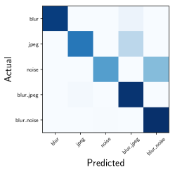
Fig. 5: Mean confusion matrix across 100 train-test splits using ResNet-50 deep features and 9-NN classifier on the LIVEMD database only for distortion type recognition.

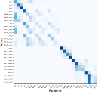
Fig. 6: Mean confusion matrix across 100 train-test splits using ResNet-50 deep features and 9-NN classifier on the LIVEMD database for multiple distortion types and severity level recognition.

7 Conclusions

In this work, starting from the previous works that have shown how perceptual similarity is an emergent property shared across deep visual representations, we analyze the capability of deep visual representations to intrinsically characterize different types of image distortions.

In the first experiment we generated a number of synthetically distorted images by applying three mainstream distortion types to the LIVE database and then we analyzed the features extracted from different layers of different deep network architectures. From the results of this experiment we observed that a PCA-reduced 2-dimensional representation of the features extracted from a given layer permits to efficiently separate types of distortions in the feature space.

As a second experiment we evaluated the use of features taken from the layer that better separated image distortions for two different tasks: reduced-reference image quality assessment, and distortion type and severity levels recognition on both single and multiple distortion databases. The results obtained in this second experiment showed that deep visual representations can be exploited even in an unsupervised way to efficiently recognize various image distortion types and severity levels.

Appendix

Appendix A Quantitative results

A.1 Analysis

In this Section we provide more details about the experiments we conducted to verify the effectiveness of deep features for image distortion characterization.

Does the capability of discriminating distortions belong to the network architecture or it depends on the network weights?

In this experiment images are encoded by using deep features extracted from randomly initialized networks. For statistical significance we compute the final distortions separability index for each layer by averaging the scores obtained for 100 network re-initializations. Table 7 depicts the resulting distortions separability indices for each layer of the considered networks. Scores are definitely lower than the ones obtained in the experiment exploiting deep features extracted from the networks pre-trained on ImageNet (see first paragraph of Section 5). This indicates that the degree of separability of images affected by diverse distortions is limited. The ranks of layers per network are completely different from the ones obtained for pre-trained networks, but as it is possible to see the standard deviation of scores among layers is small.

Table 7: Distortions separability indices for each layer of the considered networks randomly initialized. The indices are calculated by combining three internal cluster validity indices and are included in the interval [0,1], in which the highest scores (in green) indicate a high separability of the types of distortions, while the low scores (in red) represent levels not able to separate the clusters that are formed to discriminate the different distortions.

Network	Layer
AlexNet	conv1	conv2	conv3	conv4	conv5
	0.3921	0.5111	0.5327	0.5359	0.5351
Inception-v3	2a3x3	3b1x1	4a3x3	mixed5b	mixed5c	mixed5d	mixed6a	mixed6b	mixed6c	mixed6d	mixed6e	mixed7a	mixed7b	mixed7c
	0.4075	0.4168	0.4250	0.4285	0.4353	0.4415	0.4379	0.4333	0.4372	0.4272	0.4284	0.4223	0.4292	0.3708
ResNet-50	conv1	layer1	layer2	layer3	layer4
	0.3943	0.5418	0.5530	0.5489	0.5565
SqueezeNet-v1.1	conv1	fire1	fire2	fire3	fire4	fire5	fire6	fire7	fire8
	0.3928	0.5159	0.5238	0.5703	0.5712	0.5809	0.5796	0.5928	0.6621
VGG-16	conv11	conv12	conv21	conv22	conv31	conv32	conv33	conv41	conv42	conv43	conv51	conv52	conv53
	0.3944	0.4069	0.5058	0.5088	0.5577	0.5621	0.5618	0.5745	0.5780	0.5765	0.5823	0.5850	0.5853

Can the removal of semantics from the visual representation of the image emphasize the distortion encoding?

In this experiment we want to understand if the separability property of clusters in the deep feature space is influenced by the content of the images. For doing that, we subtract in channel dimension the vector of features, of size $1\times c_{l}$, of the reference image to the feature vector of the distorted image. In Table 8 we report the results of this experiment, which indicate that the semantics does not affect the rank of the layers for AlexNet, VGG-16, as well as for ResNet-50 which, however, presents an increase in the distortions separability index for the best layer (i.e. layer1). This may be due to the presence of skip connections that carry low-level information from previous layers. Both Inception-v3 and SqueezeNet-v1.1 obtain a different rank of layers with also lower scores for the distortions separability index.

Table 8: Distortions separability indices for each layer of the considered networks pre-trained on ImageNet without semantics. To isolate the signal encoding the semantics we subtract the deep features encoding the reference image from the deep features for the distorted one. The indices are calculated by combining three internal cluster validity indices and are included in the interval [0,1], in which the highest scores (in green) indicate a high separability of the types of distortions, while the low scores (in red) represent levels not able to separate the clusters that are formed to discriminate the different distortions.

Network	Layer
AlexNet	conv1	conv2	conv3	conv4	conv5
	0.5360	0.5810	0.5183	0.4544	0.4622
Inception-v3	2a3x3	3b1x1	4a3x3	mixed5b	mixed5c	mixed5d	mixed6a	mixed6b	mixed6c	mixed6d	mixed6e	mixed7a	mixed7b	mixed7c
	0.3428	0.4052	0.4161	0.3938	0.3983	0.4009	0.4375	0.4675	0.4608	0.4713	0.4550	0.4540	0.5579	0.5619
ResNet-50	conv1	layer1	layer2	layer3	layer4
	0.3935	0.7791	0.6216	0.4686	0.4686
SqueezeNet-v1.1	conv1	fire1	fire2	fire3	fire4	fire5	fire6	fire7	fire8
	0.4904	0.6268	0.6547	0.6442	0.6655	0.6596	0.5942	0.6121	0.7132
VGG-16	conv11	conv12	conv21	conv22	conv31	conv32	conv33	conv41	conv42	conv43	conv51	conv52	conv53
	0.5040	0.6258	0.6459	0.6905	0.6480	0.6200	0.5331	0.5735	0.5452	0.4962	0.4494	0.4133	0.3889

A.2 Applications

In this Section we provide a more detailed analysis of the correlation between the estimated quality scores and the ground-truth ones.

Reduced-Reference Image Quality Assessment

In Table 9 we report results for the reduced-reference image quality assessment task. We show correlations estimated for each image distortion separately, i.e. additive white Gaussian noise (AWGN), Gaussian blur and JPEG compression, on each of the four image quality databases considered (CSIQ, LIVE, TID2008, and TID2013).

Table 9: Median and mean SROCC and PLCC values across 100 train-test random splits on different types of distortions on CSIQ, LIVE, TID2008, and TID2013 databases for the considered networks.

Database	Network	Dist. type	Median		Mean
			SROCC	LCC	SROCC	LCC
CSIQ	AlexNet	AWGN	0.9533	0.9527	0.9532	0.9523
	Inception-v3		0.9168	0.9174	0.9110	0.9103
	ResNet-50		0.9359	0.9374	0.9347	0.9354
	SqueezeNet-v1.1		0.9040	0.8772	0.8976	0.8733
	VGG-16		0.9416	0.9432	0.9394	0.9410
	AlexNet	GBlur	0.8982	0.8540	0.8968	0.8568
	Inception-v3		0.9702	0.9679	0.9654	0.9630
	ResNet-50		0.9617	0.9614	0.9572	0.9555
	SqueezeNet-v1.1		0.9519	0.9366	0.9501	0.9353
	VGG-16		0.8977	0.8625	0.8837	0.8444
	AlexNet	JPEG	0.9306	0.9462	0.9235	0.9324
	Inception-v3		0.9563	0.9470	0.9493	0.9413
	ResNet-50		0.9497	0.9518	0.9434	0.9461
	SqueezeNet-v1.1		0.9153	0.9373	0.9116	0.9324
	VGG-16		0.9221	0.9245	0.9136	0.9101
LIVE	AlexNet	AWGN	0.9844	0.9566	0.9838	0.9561
	Inception-v3		0.9266	0.9262	0.9206	0.9210
	ResNet-50		0.9742	0.9822	0.9727	0.9805
	SqueezeNet-v1.1		0.9506	0.9531	0.9427	0.9331
	VGG-16		0.9782	0.9641	0.9777	0.9637
	AlexNet	GBlur	0.8598	0.8501	0.8325	0.8053
	Inception-v3		0.9377	0.9433	0.9368	0.9400
	ResNet-50		0.9399	0.9384	0.9377	0.9323
	SqueezeNet-v1.1		0.9190	0.8940	0.9123	0.8929
	VGG-16		0.8407	0.8085	0.8355	0.8000
	AlexNet	JPEG	0.9518	0.9623	0.9455	0.9462
	Inception-v3		0.9325	0.9308	0.9301	0.9289
	ResNet-50		0.9546	0.9563	0.9458	0.9473
	SqueezeNet-v1.1		0.9254	0.9136	0.9207	0.9130
	VGG-16		0.9149	0.9163	0.9079	0.9091
TID2008	AlexNet	AWGN	0.9395	0.9387	0.9358	0.9356
	Inception-v3		0.7549	0.7511	0.7500	0.7495
	ResNet-50		0.9278	0.9237	0.9263	0.9206
	SqueezeNet-v1.1		0.7714	0.7379	0.7736	0.7456
	VGG-16		0.9485	0.9470	0.9407	0.9375
	AlexNet	GBlur	0.8977	0.8705	0.8463	0.8058
	Inception-v3		0.9639	0.9633	0.9520	0.9502
	ResNet-50		0.9364	0.9372	0.9306	0.9339
	SqueezeNet-v1.1		0.8722	0.8666	0.8637	0.8533
	VGG-16		0.9263	0.9152	0.8692	0.8292
	AlexNet	JPEG	0.9459	0.9576	0.9449	0.9496
	Inception-v3		0.8845	0.8998	0.8701	0.8833
	ResNet-50		0.9308	0.9592	0.9285	0.9485
	SqueezeNet-v1.1		0.8647	0.8742	0.8352	0.8367
	VGG-16		0.9289	0.9452	0.9217	0.9187
TID2013	AlexNet	AWGN	0.9521	0.9489	0.9470	0.9469
	Inception-v3		0.8332	0.8291	0.8194	0.8147
	ResNet-50		0.9300	0.9317	0.9257	0.9268
	SqueezeNet-v1.1		0.8246	0.8111	0.8269	0.8109
	VGG-16		0.9434	0.9495	0.9380	0.9438
	AlexNet	GBlur	0.9446	0.9070	0.9163	0.8779
	Inception-v3		0.9646	0.9629	0.9584	0.9565
	ResNet-50		0.9533	0.9593	0.9518	0.9563
	SqueezeNet-v1.1		0.9069	0.8992	0.8966	0.8872
	VGG-16		0.9500	0.9555	0.9178	0.8893
	AlexNet	JPEG	0.9615	0.9752	0.9615	0.9688
	Inception-v3		0.9136	0.9249	0.8949	0.9074
	ResNet-50		0.9377	0.9592	0.9327	0.9508
	SqueezeNet-v1.1		0.8932	0.9075	0.8667	0.8623
	VGG-16		0.9500	0.9557	0.9460	0.9430

References

- Arbelaitz et al. (2013) Arbelaitz, O., Gurrutxaga, I., Muguerza, J., Pérez, J.M., Perona, I., 2013. An extensive comparative study of cluster validity indices. Elsevier Pattern Recognition 46, 243–256.
- Caliński and Harabasz (1974) Caliński, T., Harabasz, J., 1974. A dendrite method for cluster analysis. Communications in Statistics-theory and Methods 3, 1–27.
- van Craenendonck and Blockeel (2015) van Craenendonck, T., Blockeel, H., 2015. Using internal validity measures to compare clustering algorithms, in: ICML-W.
- Davies and Bouldin (1979) Davies, D.L., Bouldin, D.W., 1979. A cluster separation measure. IEEE Transactions on Pattern Analysis and Machine Intelligence PAMI-1, 224–227.
- Gatys et al. (2015a) Gatys, L., Ecker, A.S., Bethge, M., 2015a. Texture synthesis using convolutional neural networks, in: NIPS, pp. 262–270.
- Gatys et al. (2015b) Gatys, L.A., Ecker, A.S., Bethge, M., 2015b. A neural algorithm of artistic style. arXiv preprint arXiv:1508.06576 .
- He et al. (2016) He, K., Zhang, X., Ren, S., Sun, J., 2016. Deep residual learning for image recognition, in: CVPR, IEEE. pp. 770–778.
- Huh et al. (2016) Huh, M., Agrawal, P., Efros, A.A., 2016. What makes imagenet good for transfer learning? arXiv preprint arXiv:1608.08614 .
- Iandola et al. (2016) Iandola, F.N., Han, S., Moskewicz, M.W., Ashraf, K., Dally, W.J., Keutzer, K., 2016. Squeezenet: Alexnet-level accuracy with 50x fewer parameters and¡ 0.5 mb model size. arXiv preprint arXiv:1602.07360 .
- Jayaraman et al. (2012) Jayaraman, D., Mittal, A., Moorthy, A.K., Bovik, A.C., 2012. Objective quality assessment of multiply distorted images, in: Asilomar Conference on Signals, Systems and Computers, IEEE. pp. 1693–1697.
- Johnson et al. (2016) Johnson, J., Alahi, A., Fei-Fei, L., 2016. Perceptual losses for real-time style transfer and super-resolution, in: ECCV, Springer. pp. 694–711.
- Krizhevsky et al. (2012) Krizhevsky, A., Sutskever, I., Hinton, G.E., 2012. Imagenet classification with deep convolutional neural networks, in: NIPS, pp. 1097–1105.
- Larson and Chandler (2010) Larson, E.C., Chandler, D.M., 2010. Most apparent distortion: full-reference image quality assessment and the role of strategy. Journal of Electronic Imaging 19, 011006–011006.
- Mahendran and Vedaldi (2015) Mahendran, A., Vedaldi, A., 2015. Understanding deep image representations by inverting them, in: CVPR, IEEE. pp. 5188–5196.
- Paszke et al. (2017) Paszke, A., Gross, S., Chintala, S., Chanan, G., Yang, E., DeVito, Z., Lin, Z., Desmaison, A., Antiga, L., Lerer, A., 2017. Automatic differentiation in pytorch .
- Ponomarenko et al. (2013) Ponomarenko, N., Ieremeiev, O., Lukin, V., Egiazarian, K., Jin, L., Astola, J., Vozel, B., Chehdi, K., Carli, M., Battisti, F., et al., 2013. Color image database tid2013: Peculiarities and preliminary results, in: European Workshop on Visual Information Processing (EUVIP), IEEE. pp. 106–111.
- Ponomarenko et al. (2009) Ponomarenko, N., Lukin, V., Zelensky, A., Egiazarian, K., Carli, M., Battisti, F., 2009. Tid2008-a database for evaluation of full-reference visual quality assessment metrics. Advances of Modern Radioelectronics 10, 30–45.
- Rousseeuw (1987) Rousseeuw, P.J., 1987. Silhouettes: a graphical aid to the interpretation and validation of cluster analysis. Journal of computational and applied mathematics 20, 53–65.
- Russakovsky et al. (2015) Russakovsky, O., Deng, J., Su, H., Krause, J., Satheesh, S., Ma, S., Huang, Z., Karpathy, A., Khosla, A., Bernstein, M., et al., 2015. Imagenet large scale visual recognition challenge. International Journal of Computer Vision 115, 211–252.
- Sharif Razavian et al. (2014) Sharif Razavian, A., Azizpour, H., Sullivan, J., Carlsson, S., 2014. Cnn features off-the-shelf: an astounding baseline for recognition, in: CVPR-W, pp. 806–813.
- Sheikh (2005) Sheikh, H., 2005. Live image quality assessment database release 2. http://live.ece.utexas.edu/research/quality .
- Simonyan et al. (2013) Simonyan, K., Vedaldi, A., Zisserman, A., 2013. Deep inside convolutional networks: Visualising image classification models and saliency maps, in: ICLR-W.
- Simonyan and Zisserman (2014) Simonyan, K., Zisserman, A., 2014. Very deep convolutional networks for large-scale image recognition. arXiv preprint arXiv:1409.1556 .
- Szegedy et al. (2016) Szegedy, C., Vanhoucke, V., Ioffe, S., Shlens, J., Wojna, Z., 2016. Rethinking the inception architecture for computer vision, in: CVPR, IEEE. pp. 2818–2826.
- Virtanen et al. (2019) Virtanen, P., Gommers, R., Oliphant, T.E., Haberland, M., Reddy, T., Cournapeau, D., Burovski, E., Peterson, P., Weckesser, W., Bright, J., van der Walt, S.J., Brett, M., Wilson, J., Jarrod Millman, K., Mayorov, N., Nelson, A.R.J., Jones, E., Kern, R., Larson, E., Carey, C., Polat, İ., Feng, Y., Moore, E.W., Vand erPlas, J., Laxalde, D., Perktold, J., Cimrman, R., Henriksen, I., Quintero, E.A., Harris, C.R., Archibald, A.M., Ribeiro, A.H., Pedregosa, F., van Mulbregt, P., Contributors, S…, 2019. SciPy 1.0–Fundamental Algorithms for Scientific Computing in Python. arXiv e-prints , arXiv:1907.10121.
- Wang and Bovik (2006) Wang, Z., Bovik, A.C., 2006. Modern image quality assessment. Synthesis Lectures on Image, Video, and Multimedia Processing 2, 1–156.
- Wang and Bovik (2011) Wang, Z., Bovik, A.C., 2011. Reduced-and no-reference image quality assessment. IEEE Signal Processing Magazine 28, 29–40.
- Wang et al. (2004) Wang, Z., Bovik, A.C., Sheikh, H.R., Simoncelli, E.P., et al., 2004. Image quality assessment: from error visibility to structural similarity. IEEE Transactions on Image Processing 13, 600–612.
- Wold et al. (1987) Wold, S., Esbensen, K., Geladi, P., 1987. Principal component analysis. Chemometrics and intelligent laboratory systems 2, 37–52.
- Yosinski et al. (2015) Yosinski, J., Clune, J., Nguyen, A., Fuchs, T., Lipson, H., 2015. Understanding neural networks through deep visualization, in: ICML-W.
- Zhang et al. (2018) Zhang, R., Isola, P., Efros, A.A., Shechtman, E., Wang, O., 2018. The unreasonable effectiveness of deep features as a perceptual metric, in: CVPR, IEEE. pp. 586–595.
- Zhang et al. (2017) Zhang, Y., Phan, T.D., Chandler, D.M., 2017. Reduced-reference image quality assessment based on distortion families of local perceived sharpness. Elsevier Signal Processing: Image Communication 55, 130–145.