Asymptotic Behavior of the Subordinated Traveling Waves

Abstract

In this paper we investigate the long-time behavior of the subordination of the constant speed traveling waves by a general class of kernels. We use the Feller–Karamata Tauberian theorem in order to study the long-time behavior of the upper and lower wave. As a result we obtain the long-time behavior for the propagation of the front of the wave.

Keywords General fractional derivative, subordination principle, Karamata-Tauberian theorem, traveling waves.

1 Introduction

1.1 Object of Study

Traveling waves form a class of functions which are solutions for different types of equations. We have in mind in particular the fractional kinetic corresponding to the initial interacting particle system of the Bolker-Pacala model in ecology, see [FKKK15] and references therein for more details. The present paper is dedicated to study the long-time (or asymptotic) behavior of the propagation of the front of the subordinated travelling waves. By a subordination of a solution $u(x,t)$ by a density function $G_{t}(\tau)$, $t,\tau>0$ we mean the function $v(x,t)$ defined by

$$v(x,t):=\int_{0}^{\infty}u(x,\tau)G_{t}(\tau)\,\mathrm{d}\tau.$$

The interpretation of the subordination $v(x,t)$ (also called subordination identity or subordination principle) is as follows. If the function $u(x,t)$ satisfies an evolution equation (say first order time derivative) then under certain conditions, $v(x,t)$ satisfies the same type of evolution equation as $u(x,t)$ with the first order time derivative replaced by a fractional time derivative. In particular, the subordination principle holds for linear PDEs. The fractional derivative appearing as a result of subordination is related to the density function $G_{t}(\tau)$. In this paper we study three classes (see (C1), (C2), and (C3) below) leading to different type of fractional derivatives. These fractional derivatives were widely used in physics for modeling slow relaxation and diffusion processes, see for example [MK00, MK04, Mai10]. As a simple example consider the equation

$$\big{(}\mathbb{D}_{t}^{\alpha}u_{\lambda}\big{)}(t)=-\lambda u_{\lambda}(t),\quad t>0,\quad u(0)=1,$$ (1.1)

where $0<\alpha<1$ and $\mathbb{D}_{t}^{\alpha}$ denotes the Caputo-Dzhrbashyan fractional derivative , see (2.11) for details. It is well known (see for example [KST06]) that the solution of equation (1.1) is given in terms of the Mittag-Leffler function $E_{\alpha}$, namely

$$u_{\lambda}(t)=E_{\alpha}(-\lambda t^{\alpha}).$$

It follows from the properties of the Mittag-Leffler function (see [GKMR14]) that $u_{\lambda}(t)\sim Ct^{-\alpha}$ as $t\to\infty,\;C>0$. Here the simbol $\sim$ means that if $f\sim g$ as $t\to\infty$, then $\lim_{t\to\infty}\frac{f(t)}{g(t)}=1$. In addition, there is a density function $G_{t}^{\alpha}(\tau)$ such that $u_{\lambda}(t)$ is a subordination, more precisely

$$u_{\lambda}(t)=\int_{0}^{\infty}e^{-\lambda\tau}G_{t}^{\alpha}(\tau)\,\mathrm{d}\tau,$$

see Proposition 2 below for more details of $G_{t}^{\alpha}(\tau)$. Note that if we replace $\mathbb{D}_{t}^{\alpha}$ by $\frac{\mathrm{d}}{\mathrm{d}t}$ in equation (1.1), then $e^{-\lambda t}$ is the solution of that equation.

1.2 Description of the Results

A monotone traveling wave $u(x,t)$ with velocity $v$ in given by a profile function $\psi:\mathbb{R}\longrightarrow[0,1]$ as $u(x,t)=\psi(x-vt)$, $t\geq 0$. Without lost of generality we assume that the profile function $\psi$ satisfies

$$\lim_{t\to-\infty}\psi(t)=1\qquad\mathrm{and}\qquad\lim_{t\to\infty}\psi(t)=0.$$

For each $\varepsilon>0$ there exist $x_{\varepsilon}^{-},x_{\varepsilon}^{+}\in\mathbb{R}$ such that

$$u(x,t)<\varepsilon,\;\forall x>x_{\varepsilon}^{+}\quad\mathrm{and}\quad u(x,t)>1-\varepsilon,\;\forall x<x_{\varepsilon}^{-}.$$

This allow us to obtain a lower wave $u_{\varepsilon}^{-}(x,t)$ and upper wave $u_{\varepsilon}^{+}(x,t)$ such that the following chain of inequalities hold

$$u_{\varepsilon}^{-}(x,t)\leq u(x,t)\leq u_{\varepsilon}^{+}(x,t).$$

Both the lower and upper wave have an explicitly expression, see Section 3 below for details. Hence, we obtain the chain of inequalities for the subordination

$$u_{\varepsilon}^{E,-}(x,t)\leq u^{E}(x,t)\leq u_{\varepsilon}^{E,+}(x,t).$$

The subordination is given with respect to the density of the inverse $E$ of a subordinator.

1.3 Motivation: Fractional Kinetic

One particular way to obtain kinetic equations for densities is the following, see e.g., [FKK10] for details. Let us consider a Markov stochastic dynamics for a continuous interacting particle system in $\mathbb{R}^{d}$. The state evolution of this system may be described by means of a hierarchical system of evolution equations for correlation functions. In a mesoscopic scaling limit (e.g., in Vlasov type scaling) we arrive in the so-called kinetic hierarchy for correlation functions. Note that, in general, this hierarchy is not related anymore to a Markov dynamics. But the key property of the kinetic hierarchy is what is called the chaos preservation in physical literature. In the mathematical language, it means the following. If we start our system after the scaling with a Poisson initial measure $\pi_{\rho}$ with the intensity measure $\mathrm{d}\sigma(x)=\rho(x)\,\mathrm{d}x$, then in the course of evolutions the state of the system will be again a Poisson measure $\pi_{\rho_{t}}$ and there exists a non-linear operator $V$ such that the density $\rho_{t}(x)$ satisfy the non-linear equation

$$\frac{\partial}{\partial t}\rho_{t}(x)=V(\rho_{t})(x),\quad x\in\mathbb{R}^{d}$$

with the initial data $\rho_{0}(x)=\rho(x)$. This equation is called the kinetic equation for the considered stochastic dynamics of an infinite particle systems. We would like to stress that the kinetic equation is only one particular byproduct of the kinetic hierarchy which may be considered as a new important system of equations describing the dynamics, see comments by H. Spohn in [Spo80].

Let us consider a random time change in the initial Markov dynamics. Then we have a hierarchical system of evolution equations with a general fractional derivative in time corresponding to the random time change, see [KKdS20, KK17]. After a scaling we obtain a kinetic hierarchy which is the same as before but with generalized time derivatives instead of usual ones. This new hierarchy does not preserve anymore the chaos property. But due to general subordination principle the solution to the fractional kinetic hierarchy is nothing but the subordination of the solution to the initial kinetic hierarchy by a particular kernel associated with the random time. The latter is deeply related to the linear character of the evolution in the kinetic hierarchies. As a consequence, we have the evolution of the density in the fractional dynamics which is nothing but the subordination of the evolution of the density corresponding to the initial kinetic equation. Therefore, the kinetic dynamics of the density in the fractional time is just the transformation of the solution to the kinetic equation in the physical time. This statement supports our doubts that the study of non-linear kinetic equations with fractional derivatives may be justified by arguments coming from physical background. Of course, we can consider non-linear evolution equations with fractional derivatives as mathematical objects. But the physical sense of their solutions remain an open question.

For several particular models of Markov dynamics we already derived and studied the related kinetic equations, see [FKK10, FKK11, FKKL11]. In particular, for certain class of such equation we obtained the existence of solutions in the form of traveling waves, see [FKT19c, FKT19a]. There appears a natural question about the properties of subordinated solutions in the case of traveling waves. The physical sense of the fractional time may be related to a friction included in the initial system. From the point of view of such interpretation we shall expect that the motion of the subordinated wave shall be slower comparing with the initial one. Actually, we will show that this hypothesis may be justified for several classes of random time changes.

2 Preliminaries

In this section we introduce the general framework we work with. More precisely, we will use the concept of general fractional derivative (GFD) associated to a kernel $k\in L_{\mathrm{loc}}^{1}(\mathbb{R}_{+})$, see [Koc11]. We consider three classes of admissible kernels $k$ characterized in terms of their Laplace transforms $\mathcal{K}(\lambda)$ as $\lambda\to 0$, see (C1), (C2) and (C3) (C1) below.

Let $S=\{S(t),\;t\geq 0\}$ be a subordinator without drift, that is, a process with stationary and independent non-negative increments starting from $0$, see [Ber96] for more details. The Laplace transform of $S(t)$, $t\geq 0$ is expressed as

$$\mathbb{E}(e^{-\lambda S(t)})=e^{-t\Phi(\lambda)},\quad\lambda\geq 0,$$

where $\Phi:[0,\infty)\longrightarrow[0,\infty)$ is called the Laplace exponent which admits the representation

$$\Phi(\lambda)=\int_{(0,\infty)}(1-e^{-\lambda\tau})\,d\sigma(\tau).$$ (2.1)

The measure $\sigma$ is called Lévy measure, has support in $[0,\infty)$ and fulfills

$$\int_{(0,\infty)}(1\wedge\tau)\,\mathrm{d}\sigma(\tau)<\infty.$$ (2.2)

In what follows we assume that the Lévy measure $\sigma$ satisfy

$$\sigma(0,\infty)=\infty.$$ (2.3)

Given the Lévy measure $\sigma$, we define the function $k$ by

$$k:(0,\infty)\longrightarrow(0,\infty),\;t\mapsto k(t):=\sigma\big{(}(t,\infty)\big{)}$$ (2.4)

and denote its Laplace transform by $\mathcal{K}$, that is, for any $\lambda\geq 0$ one has

$$\mathcal{K}(\lambda):=\int_{0}^{\infty}e^{-\lambda t}k(t)\,\mathrm{d}t.$$ (2.5)

The function $\mathcal{K}$ is expressed in terms of the Laplace exponent $\Phi$ as

$$\Phi(\lambda)=\lambda\mathcal{K}(\lambda),\quad\forall\lambda>0.$$ (2.6)

Example 1.

1. The classical example of a subordinator $S$ is the so-called $\alpha$-stable process $\alpha\in(0,1)$ with Laplace exponent $\Phi(\lambda)=\lambda^{\alpha}$ and Lévy measure $d\sigma(\tau)=\frac{\alpha}{\Gamma(1-\alpha)}\tau^{-1-\alpha}\,d\tau.$

2. The Gamma process $Y^{(a,b)}$ with parameters $a,b>0$ is another example of a subordinator with Laplace exponent $\Phi_{(a,b)}(\lambda)=a\log\left(1+\frac{\lambda}{b}\right)$ and Lévy measure $d\sigma(\tau)=a\tau^{-1}e^{-b\tau}\,d\tau.$

Let $E$ be the inverse process of the subordinator $S$, that is,

$$E(t):=\inf\{s\geq 0:\;S(s)\geq t\}=\sup\{s\geq 0:\;S(s)\leq t\}.$$ (2.7)

For any $t\geq 0$ we denote by $G_{t}^{k}(\tau)\equiv G_{t}(\tau)$, $\tau\geq 0$ the marginal density of $E(t)$ or, equivalently

$$G_{t}(\tau)\,\mathrm{d}\tau=\partial_{\tau}P(E(t)\leq\tau)=\partial_{\tau}P(S(\tau)\geq t)=-\partial_{\tau}P(S(\tau)<t).$$

As the density $G_{t}(\tau)$ plays an important role in the analysis below here we collect some important properties.

Proposition 2 (cf. Prop. 1(a) in [Bin71]).

If $S$ is the $\alpha$-stable process, $\alpha\in(0,1)$, then the inverse process $E(t)$ has a Mittag-Leffler distribution, namely

$$\mathbb{E}(e^{-\lambda E(t)})=\int_{0}^{\infty}e^{-t\tau}G_{t}(\tau)\,\mathrm{d}\tau=\sum_{n=0}^{\infty}\frac{(-\lambda t^{\alpha})^{n}}{\Gamma(n\alpha+1)}=E_{\alpha}(-\lambda t^{\alpha}).$$ (2.8)

Here $E_{\alpha}$ is the Mittag-Leffler function with index $\alpha$, see [GKMR14].

Remark 3.

1. It follows from the asymptotic behavior of the Mittag-Leffler function $E_{\alpha}$ that $\mathbb{E}(e^{-\lambda E(t)})\sim Ct^{-\alpha}$ as $t\to\infty$.

2. It follows from the properties of the Mittag-Leffler function $E_{\alpha}$, that the density $G_{t}(\tau)$ is given in terms of the Wright function $W_{\mu,\nu}$, namely $G_{t}(\tau)=t^{-\alpha}W_{-\alpha,1-\alpha}(\tau t^{-\alpha})$, see [GLM99] for more details.

For a general subordinator, the following lemma determines the $t$-Laplace transform of $G_{t}(\tau)$, with $k$ and $\mathcal{K}$ given in (2.4) and (2.5), respectively. For the proof see [Koc11].

Lemma 4.

The $t$-Laplace transform of the density $G_{t}(\tau)$ is given by

$$\int_{0}^{\infty}e^{-\lambda t}G_{t}(\tau)\,\mathrm{d}t=\mathcal{K}(\lambda)e^{-\tau\lambda\mathcal{K}(\lambda)}.$$ (2.9)

The double ($\tau,t$)-Laplace transform of $G_{t}(\tau)$ is

$$\int_{0}^{\infty}\int_{0}^{\infty}e^{-p\tau}e^{-\lambda t}G_{t}(\tau)\,\mathrm{d}t\,\mathrm{d}\tau=\frac{\mathcal{K}(\lambda)}{\lambda\mathcal{K}(\lambda)+p}.$$ (2.10)

For any $\alpha\in(0,1)$ the Caputo-Dzhrbashyan fractional derivative of order $\alpha$ of a function $u$ is defined by (see e.g., [KST06] and references therein)

$$\big{(}\mathbb{D}_{t}^{\alpha}u\big{)}(t)=\frac{d}{dt}\int_{0}^{t}k(t-\tau)u(\tau)\,\mathrm{d}\tau-k(t)u(0),\quad t>0,$$ (2.11)

where

$$k(t)=\frac{t^{-\alpha}}{\Gamma(1-\alpha)},\;t>0.$$

More generally, we consider differential-convolution operators

$$\big{(}\mathbb{D}_{t}^{(k)}u\big{)}(t)=\frac{d}{dt}\int_{0}^{t}k(t-\tau)u(\tau)\,\mathrm{d}\tau-k(t)u(0),\;t>0,$$ (2.12)

where $k\in L_{\mathrm{loc}}^{1}(\mathbb{R}_{+})$ is a nonnegative kernel. The distributed order derivative $\mathbb{D}_{t}^{(\mu)}$ is an example of such operator, corresponding to

$$k(t)=\int_{0}^{1}\frac{t^{-\tau}}{\Gamma(1-\tau)}\mu(\tau)\,\mathrm{d}\tau,\quad t>0,$$ (2.13)

where $\mu(\tau)$, $0\leq\tau\leq 1$ is a positive weight function on $[0,1]$, see [APZ09, DGB08, GU05, Han07, Koc08, MS06].

From now on $L$ always denotes a slowly varying function (SVF) at infinity (see for instance [BGT87] and [SSV12]), that is,

$$\lim_{x\to\infty}\frac{L(\lambda x)}{L(x)}=1,\qquad\mathrm{for\;any\;}\lambda>0,$$

while $C$, $C_{\pm}$ are constants whose values are unimportant, and which may change from line to line.

In the following we consider three classes of admissible kernels $k\in L_{\mathrm{loc}}^{1}(\mathbb{R}_{+})$, characterized in terms of their Laplace transforms $\mathcal{K}(\lambda)$ as $\lambda\to 0$ (i.e., as local conditions):

$$\mathcal{K}(\lambda)\sim\lambda^{\alpha-1},\quad 0<\alpha<1.$$ (C1)

$$\mathcal{K}(\lambda)\sim\lambda^{-1}L\left(\frac{1}{\lambda}\right),\quad L(y):=\mu(0)\log(y)^{-1}.$$ (C2)

$$\mathcal{K}(\lambda)\sim\lambda^{-1}L\left(\frac{1}{\lambda}\right),\quad L(y):=C\log(y)^{-1-s},\;s>0,\;C>0.$$ (C3)

We would like to emphasize that these three classes of kernels lead to different differential-convolution operators. In particular, the Caputo-Djrbashian fractional derivative (C1) and distributed order derivatives (C2), (C3). In the next section we study the long-time behavior of the subordination of the constant speed traveling wave corresponding to these differential-convolution operators. Working in such generality a price must be paid, namely the replacement of the fundamental solution by its Cesaro mean. This is the key technical observation that underlies the analysis of several different model situations.

3 Long-time Behavior of the Subordination of Traveling Waves

A monotone traveling wave $u(x,t)$, $t\geq 0$, $x\in\mathbb{R}$ with velocity $v>0$ is defined by a profile function $\psi:\mathbb{R}\longrightarrow[0,1]$ which is a continuous monotonically decreasing function such that

$$\lim_{x\to-\infty}\psi(x)=1,\qquad\lim_{x\to\infty}\psi(x)=0,$$

and $u(x,t)=\psi(x-vt)$, $t\geq 0$ for almost all $x\in\mathbb{R}$. For each $\varepsilon>0$ and $t>0$ introduce $x_{\varepsilon}^{-},x_{\varepsilon}^{+}\in\mathbb{R}$ as

$$\forall x>x_{\varepsilon}^{+},\;\;u(x,t)<\varepsilon\quad\mathrm{and}\quad\forall x<x_{\varepsilon}^{-},\;\;u(x,t)>1-\varepsilon$$

and consider the two-side estimate of $u(x,t)$ for any $x\in\mathbb{R}$ and $t\geq 0$

$$u_{\varepsilon}^{-}(x,t)\leq u(x,t)\leq u_{\varepsilon}^{+}(x,t),$$ (3.1)

where

$$u_{\varepsilon}^{+}(x,t) := \mathbbm{1}_{(-\infty,x_{\varepsilon}^{+}]}(x-vt)+\varepsilon\mathbbm{1}_{[x_{\varepsilon}^{+},\infty)}(x-vt),$$

$$u_{\varepsilon}^{-}(x,t) := (1-\varepsilon)\mathbbm{1}_{(-\infty,x_{\varepsilon}^{-}]}(x-vt).$$

The functions $u_{\varepsilon}^{-}(x,t)$ and $u_{\varepsilon}^{+}(x,t)$ we will call lower and upper waves, respectively, see Figure 1.

3.1 Subordination of the Traveling Wave

Consider the solutions of the evolution equations

$$\frac{\partial}{\partial t}u_{1}(x,t) = (Au_{1})(x,t)$$ (3.2)

$$\big{(}\mathbb{D}_{t}^{(k)}u_{k}\big{)}(t) = (Au_{k})(x,t),$$ (3.3)

where $A$ is an operator acting in the spatial variable $x$ and the same initial conditions

$$u_{1}(x,0)=\xi(x),\qquad u_{k}(x,0)=\xi(x).$$

Then in certain conditions (e.g. $A$ closed linear operator) the solutions $u_{1}$ and $u_{k}$ satisfy the subordination identity (also known as subordination principle), that is, there exists a nonnegative function $G_{t}(\tau)$, $t,\tau>0$ such that $\int_{0}^{\infty}G_{t}(\tau)\,\mathrm{d}\tau=1$ and

$$u_{k}(x,t)=\int_{0}^{\infty}u_{1}(x,\tau)G_{t}(\tau)\,\mathrm{d}\tau.$$

aThe proper notion of solution for equations (3.2) and (3.3) were explained in [Koc11] when $A$ is the Laplace operator on $\mathbb{R}^{n}$, in [Baz00, Baz01, Baz15] in the framework of semigroups generators (for special classes of $k$) or in [Prü93] for abstract Volterra equations.

We are interested in the subordination of the traveling wave $u(x,t)$ by the density $G_{t}(\tau)$ associated to the inverse process $E$. Hence, we obtain a new function $u^{E}(x,t)$ defined by

$$u^{E}(x,t):=\int_{0}^{\infty}u(x,\tau)G_{t}(\tau)\,\mathrm{d}\tau.$$ (3.4)

The subordination of the lower and upper waves, denoted by $u^{E,-}_{\varepsilon}(x,t)$ and $u^{E,+}_{\varepsilon}(x,t)$, respectively, are defined similarly. Having in mind the chain of inequalities (3.1) we obtain the chain for the subordinated functions

$$u^{E,-}_{\varepsilon}(x,t)\leq u^{E}(x,t)\leq u^{E,+}_{\varepsilon}(x,t).$$ (3.5)

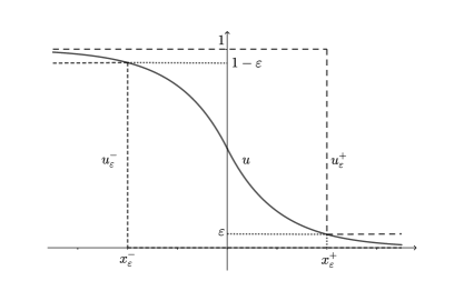
Figure 1: Traveling wave $u$, upper wave $u_{\varepsilon}^{+}$ and lower wave $u_{\varepsilon}^{-}$.

Remark 5.

The long time behavior of the function $u^{E}(x,t)$ as $t\to\infty$ may be determined, under certain conditions, by studying the behavior of its Laplace transform $\tilde{u}^{E}(x,\lambda)$ as $\lambda\to 0$, and vice versa. An important situation where such a correspondence holds is described by the Feller–Karamata Tauberian (FKT) theorem.

We state below a version of the FKT theorem which suffices for our purposes, see the monographs [BGT87, Sec. 1.7] and [Fel71, XIII, Sec. 1.5] for a more general version and proofs.

Theorem 6 (Feller–Karamata Tauberian).

Let $U:[0,\infty)\longrightarrow\mathbb{R}$ be a monotone non-decreasing right-continuous function such that

$$w(\lambda):=\int_{0}^{\infty}e^{-\lambda t}\,\mathrm{d}U(t)<\infty,\quad\forall\lambda>0.$$

If $L$ is a slowly varying function and $C,\rho\geq 0$, then the following are equivalent

$$U(t)\sim\frac{C}{\Gamma(\rho+1)}t^{\rho}L(t)\quad\mathrm{as}\;t\to\infty,$$ (3.6)

$$w(\lambda)\sim C\lambda^{-\rho}L\left(\frac{1}{\lambda}\right)\quad\mathrm{as}\;\lambda\to 0^{+}.$$ (3.7)

When $C=0$, (3.6) is to be interpreted as $U(t)=o(t^{\rho}L(t))$; similarly for (3.7).

Remark 7.

1. In general, the function $u^{E}(x,t)$ is not monotone in $t$, that will be needed to apply the Theorem 6. In addition, the Laplace transform of $u^{E}(x,t)$ can be explicitly computed only when $G_{t}(\tau)$ corresponds to the density of the inverse stable subordinator.

2. We define the $t$-increasing function

   $$\int_{0}^{t}u^{E}(x,s)\,\mathrm{d}s$$

   and then will obtain the long-time behavior for the Cesaro mean of $u^{E}(x,t)$, that is,

   $$M_{t}(u^{E}(x,\cdot)):=\frac{1}{t}\int_{0}^{t}u^{E}(x,s)\,\mathrm{d}s.$$ (3.8)

3. For any fixed time $t$, the subordinated traveling wave $u^{E}(x,t)$ is decreasing and continuous in $x$. Hence, given $\beta\in(0,1)$ there is a unique $x_{\beta}^{E}(t)\in(0,1)$ which solves the equation

   $$u^{E}(x_{\beta}^{E}(t),t)=\beta.$$

   We call $x_{\beta}^{E}(t)$ the propagation of the front of $u^{E}(x,t)$ of the level $\beta$. For a general definition of the propagation of the front of a function $u(x,t)$, which is the solution of a certain differential equation, see [FKT19b] and references therein.

The considerations in Remark 7 lead us to consider the chain of inequalities for the Cesaro means, namely

$$M_{t}(u^{E,-}_{\varepsilon}(x,\cdot))\leq M_{t}(u^{E}(x,\cdot))\leq M_{t}(u^{E,+}_{\varepsilon}(x,\cdot)).$$

Unfortunately the FKT theorem does not apply to inequalities. Hence, we study the long-time behavior of the Cesaro mean of the subordination of both the upper and lower waves separately. It turns out that both of these long-time behavior are of the same type, compare for example (3.11) and (3.19) for the class (C1). Although we are not allowed to conclude any type of long-time behavior for the Cesaro mean of our subordination travelling wave $u^{E}(x,t)$, it gives good indications and we may derive a two-side estimation for the propagation of the front which are again of the type. The results for the class (C1) are stated in Theorem 9 below, see also Theorem 11 (resp. Theorem 12) for the class (C2) (resp. class (C3)).

3.2 Long-Time Behavior: Class (C1)

3.2.1 The Subordination of the Lower Wave

We start with the lower wave, namely the subordination

$$u_{\varepsilon}^{E,-}(x,t):=(1-\varepsilon)\int_{0}^{\infty}\mathbbm{1}_{(-\infty,x_{\varepsilon}^{-}]}(x-v\tau)G_{t}(\tau)\,\mathrm{d}\tau.$$ (3.9)

If we denote by $\theta_{\varepsilon}^{-}:=\frac{x-x_{\varepsilon}^{-}}{v}$ with $x>x_{\varepsilon}^{-}$, then $u_{\varepsilon}^{E,-}(x,t)$ is given by

$$u_{\varepsilon}^{E,-}(x,t)=(1-\varepsilon)\int_{\theta_{\varepsilon}^{-}}^{\infty}G_{t}(\tau)\,\mathrm{d}\tau.$$

Computing the Laplace transform of the monotone function $v^{-}(x,t):=\int_{0}^{t}u_{\varepsilon}^{E,-}(x,s)\,\mathrm{d}s$

$$(\mathscr{L}v^{-}(x,\cdot))(\lambda) = \int_{0}^{\infty}e^{-\lambda t}\,\mathrm{d}_{t}v^{-}(x,t)=\int_{0}^{\infty}e^{-\lambda t}u^{E,-}_{\varepsilon}(x,t)\,\mathrm{d}t$$

$$= \int_{0}^{\infty}e^{-\lambda t}\int_{\theta_{\varepsilon}^{-}}^{\infty}G_{t}(\tau)\,\mathrm{d}\tau\,\mathrm{d}t.$$

Using Fubini theorem and equality (2.9) yields

$$(\mathscr{L}v^{-}(x,\cdot))(\lambda)=(1-\varepsilon)\mathcal{K}(\lambda)\int_{\theta_{\varepsilon}^{-}}^{\infty}e^{-\tau\lambda\mathcal{K}(\lambda)}\,\mathrm{d}\tau=(1-\varepsilon)\lambda^{-1}e^{-\theta_{\varepsilon}^{-}\lambda\mathcal{K}(\lambda)}.$$ (3.10)

For the class (C1) we have $\mathcal{K}(\lambda)\sim\lambda^{\alpha-1}$, $\lambda\to 0$, $0<\alpha<1$, hence

$$(\mathscr{L}v^{-}(x,\cdot))(\lambda)\sim(1-\varepsilon)\lambda^{-1}e^{-\theta_{\varepsilon}^{-}\lambda^{\alpha}}=\lambda^{-\rho}L\left(\frac{1}{\lambda}\right),\quad\lambda\to 0,$$

where $\rho=1$ and $L(y)=(1-\varepsilon)\exp(-\theta_{\varepsilon}^{-}y^{-\alpha})$ is a SVF. Then we conclude by FKT (see Theorem 6) that $v^{-}({x,t})\sim tL(t)$, $t\to\infty$ which implies the long-time behavior for the Cesaro mean of the subordination of the lower wave $u^{E,-}_{\varepsilon}(x,t)$:

$$M_{t}(u_{\varepsilon}^{E,-}(x,\cdot))=\frac{1}{t}v^{-}(x,t)\sim L(t)=(1-\varepsilon)e^{-\theta_{\varepsilon}^{-}t^{-\alpha}},\;t\to\infty.$$ (3.11)

Define the right hand side of the above by $W_{\varepsilon}^{-}(x,t)$, that is,

$$W_{\varepsilon}^{-}(x,t):=(1-\varepsilon)e^{-\theta_{\varepsilon}^{-}t^{-\alpha}}.$$

It is clear that for any fixed $x$ we have

$$W_{\varepsilon}^{-}(x,t)\to 1-\varepsilon,\quad t\to\infty$$

and fixing $t$ (recall $\theta_{\varepsilon}^{-}=\frac{x-x_{\varepsilon}^{-}}{v}$) yields

$$W_{\varepsilon}^{-}(x,t)\to 0,\quad x\to\infty.$$

To find the propagation of the front $x_{\varepsilon,\beta}^{-}(t)$ of the Cesaro mean $M_{t}(u_{\varepsilon}^{E,-}(x,\cdot))$ of the level $\beta\in(0,1-\varepsilon)$ we solve the equation

$$W_{\varepsilon}^{-}(x_{\varepsilon,\beta}^{-}(t),t)=\beta$$

to obtain

$$x_{\varepsilon,\beta}^{-}(t)\sim vt^{\alpha}\log\left(\frac{1-\varepsilon}{\beta}\right)+x_{\varepsilon}^{-}=:C_{-}t^{\alpha}+x_{\varepsilon}^{-},\quad t\to\infty.$$

So, the propagation of the front of the Cesaro mean $M_{t}(u_{\varepsilon}^{E,-}(x,\cdot))$ is $x_{\varepsilon,\beta}^{-}(t)\sim C_{-}t^{\alpha}$ as $t\to\infty$.

3.2.2 The Subordination of the Upper Wave

We are now interested in the upper wave, namely the subordination

$$u_{\varepsilon}^{E,+}(x,t) :=\int_{0}^{\infty}u^{+}_{\varepsilon}(x,\tau)G_{t}(\tau)\,\mathrm{d}\tau$$ (3.12)

$$=\int_{0}^{\infty}\mathbbm{1}_{(-\infty,x_{\varepsilon}^{+}]}(x-v\tau)G_{t}(\tau)\,\mathrm{d}\tau+\varepsilon\int_{0}^{\infty}\mathbbm{1}_{[x_{\varepsilon}^{+},\infty)}(x-v\tau)G_{t}(\tau)\,\mathrm{d}\tau$$ (3.13)

$$=:u_{\varepsilon}^{E,+,1}(x,t)+u_{\varepsilon}^{E,+,2}(x,t).$$ (3.14)

As before we study the Cesaro mean of each of the above functions, namely

$$M_{t}(u_{\varepsilon}^{E,+,1}(x,\cdot)) :=\frac{1}{t}\int_{0}^{t}u_{\varepsilon}^{E,+,1}(x,s)\,\mathrm{d}s,$$

$$M_{t}(u_{\varepsilon}^{E,+,2}(x,\cdot)) :=\frac{1}{t}\int_{0}^{t}u_{\varepsilon}^{E,+,2}(x,s)\,\mathrm{d}s.$$

If we denote by $\theta_{\varepsilon}^{+}:=\frac{x-x_{\varepsilon}^{+}}{v}$ with $x>x_{\varepsilon}^{+}$, then $u_{\varepsilon}^{E,+,1}(x,t)$ is equal to

$$u_{\varepsilon}^{E,+,1}(x,t):=\int_{\theta_{\varepsilon}^{+}}^{\infty}G_{t}(\tau)\,\mathrm{d}\tau.$$

Computing the Laplace transform of the monotone function $v^{+,1}(x,t):=\int_{0}^{t}u_{\varepsilon}^{E,+,1}(x,s)\,\mathrm{d}s$ and using (2.9) yields

$$(\mathscr{L}v^{+,1}(x,\cdot))(\lambda)=\mathcal{K}(\lambda)\int_{\theta_{\varepsilon}^{+}}^{\infty}e^{-\tau\lambda\mathcal{K}(\lambda)}\,\mathrm{d}\tau=\lambda^{-1}e^{-\theta_{\varepsilon}^{+}\lambda\mathcal{K}(\lambda)}.$$ (3.15)

A similar procedure for $v^{+,2}(x,t):=\int_{0}^{t}u_{\varepsilon}^{E,+,2}(x,s)\,\mathrm{d}s$ produces the following Laplace transform

$$(\mathscr{L}v^{+,2}(x,\cdot))(\lambda)=\varepsilon\mathcal{K}(\lambda)\int_{0}^{\theta_{\varepsilon}^{+}}e^{-\tau\lambda\mathcal{K}(\lambda)}\,\mathrm{d}\tau=\varepsilon\lambda^{-1}(1-e^{-\theta_{\varepsilon}^{+}\lambda\mathcal{K}(\lambda)}).$$ (3.16)

For the class (C1), $\mathcal{K}(\lambda)\sim\lambda^{\alpha-1}$, $\lambda\to 0$, $0<\alpha<1$, it follows from (3.15) that

$$(\mathscr{L}u_{\varepsilon}^{E,+,1}(x,\cdot))(\lambda)\sim\lambda^{-1}e^{-\theta_{\varepsilon}^{+}\lambda^{\alpha}}=\lambda^{-\rho}L\left(\frac{1}{\lambda}\right),$$

where $\rho=1$ and $L(y)=\exp(-\theta_{\varepsilon}^{+}y^{-\alpha})$ is a SVF. Then we conclude

$$M_{t}(u_{\varepsilon}^{E,+,1}(x,\cdot))\sim L(t)=e^{-\theta_{\varepsilon}^{+}t^{-\alpha}},\;t\to\infty.$$ (3.17)

For the second function $u_{\varepsilon}^{E,+,2}(x,t)$ we obtain

$$(\mathscr{L}u_{\varepsilon}^{E,+,2}(x,\cdot))(\lambda)=\varepsilon\lambda^{-1}(1-e^{-\theta_{\varepsilon}^{+}\lambda^{\alpha}})=\lambda^{-\rho}L\left(\frac{1}{\lambda}\right),$$

where $\rho=1$ and $L(y)=\varepsilon(1-\exp(-\theta_{\varepsilon}^{+}y^{-\alpha})$ is a SVF. Thus

$$M_{t}(u_{\varepsilon}^{E,+,2}(x,\cdot))\sim L(t)=\varepsilon\left(1-e^{-\theta_{\varepsilon}^{+}t^{-\alpha}}\right),\;t\to\infty.$$ (3.18)

Putting (3.17) and (3.18) together we obtain

$$M_{t}(u_{\varepsilon}^{E,+}(x,\cdot))\sim(1-\varepsilon)\exp\left(-\frac{x-x_{\varepsilon}^{+}}{v}t^{-\alpha}\right)+\varepsilon.$$ (3.19)

Define the right hand side of the above by $W_{\varepsilon}^{+}(x_{\varepsilon}^{+},t)$, that is

$$W_{\varepsilon}^{+}(x_{\varepsilon}^{+},t):=(1-\varepsilon)\exp\left(-\frac{x-x_{\varepsilon}^{+}}{v}t^{-\alpha}\right)+\varepsilon.$$

For any fixed $x$ we have

$$W_{\varepsilon}^{+}(x_{\varepsilon}^{+},t)\to 1,\quad t\to\infty$$

and if $t$ is fixed we obtain

$$W_{\varepsilon}^{+}(x_{\varepsilon}^{+},t)\to\varepsilon,\quad x\to\infty.$$

To find the propagation of the front $x_{\varepsilon,\beta}^{+}(t)$ of the Cesaro mean $M_{t}(u_{\varepsilon}^{E,+}(x,\cdot))$ of the level $\beta\in(\varepsilon,1)$ we solve the equation

$$W_{\varepsilon}^{+}(x_{\varepsilon,\beta}^{+}(t),t)=\beta$$

for $x_{\varepsilon,\beta}^{+}(t)$ and obtain

$$x_{\varepsilon,\beta}^{+}(t)=vt^{\alpha}\log\left(\frac{1-\varepsilon}{\beta-1}\right)+x_{\varepsilon}^{+}=:C_{+}t^{\alpha}+x_{\varepsilon}^{-},\quad t\to\infty.$$

So, the propagation of the front of the Cesaro mean $M_{t}(u_{\varepsilon}^{E,-}(x,t))$ of the subordinated of the upper wave is $x_{\varepsilon,\beta}^{+}(t)\sim C_{+}t^{\alpha}$ as $t\to\infty$.

Remark 8.

For any $x\in\mathbb{R}$ and $t\geq 0$ we have the following chain of inequalities, cf. (3.1)

$$u_{\varepsilon}^{E,-}(x,t)\leq u^{E}(x,t)\leq u_{\varepsilon}^{E,+}(x,t).$$

As $G_{t}(\tau)$ is a density, the same type of chain for the Cesaro mean is also valid, that is

$$M_{t}\big{(}u_{\varepsilon}^{E,-}(x,\cdot)\big{)}\leq M_{t}\big{(}u^{E}(x,\cdot)\big{)}\leq M_{t}\big{(}u_{\varepsilon}^{E,+}(x,\cdot)\big{)}.$$

If $x_{\beta}(t)\in(\varepsilon,1-\varepsilon)$ denotes the propagation of the front of the Cesaro mean $M_{t}\big{(}\psi^{E}(x,t)\big{)}$ of the level $\beta$, then the following relation between the propagation of the fronts of the level $\beta$ hold

$$C_{-}t^{\alpha}\sim x_{\varepsilon}^{-}(t)\leq x_{\beta}(t)\leq x_{\varepsilon,\beta}^{+}(t)\sim C_{+}t^{\alpha},\quad t\to\infty.$$

We have shown the following theorem.

Theorem 9.

Let $u(x,t)=\psi(x-vt)$ be a traveling wave with constant speed $v$ with two-side estimate, for any $x\in\mathbb{R}$, $t\geq 0$ and $\varepsilon>0$

$$u_{\varepsilon}^{-}(x,t)\leq u(x,t)\leq u_{\varepsilon}^{+}(x,t).$$

The subordination $u^{E}(x,t)$ of $u(x,t)$ with the density $G_{t}(\tau)$ (corresponding to the class (C1)) has Cesaro mean $M_{t}\big{(}u^{E}(x,\cdot)\big{)}$ with a propagation of the front $x_{\beta}(t)$ of the level $\beta$ that satisfies the two-side estimate, with $C_{-},C_{+}>0$

$$C_{-}t^{\alpha}\leq x_{\beta}(t)\leq C_{+}t^{\alpha}\quad\mathrm{as}\quad t\to\infty.$$

Then we have $x_{\beta}(t)\sim Ct^{\alpha}$ as $t\to\infty$ with $C>0$.

Remark 10.

In Example 5 of [DSKT18] it is shown, using a direct method, for the particular example of the inverse stable subordinator from the class (C1) the long-time behavior of the propagation of the front $x_{\beta}(t)$ is given by

$$x_{\beta}(t)=Ct^{\alpha}+o(t^{\alpha}),\quad t\to\infty.$$

This shows that when the long-time behavior exists for the subordinated wave, then the Cesaro mean gives the right result.

3.3 Long-Time Behavior: Class (C2)

3.3.1 The Subordination of the Lower Wave

Here we have $\mathcal{K}(\lambda)\sim\lambda^{-1}L(\lambda^{-1})$ as $\lambda\to 0$, where $L(y)=\mu(0)\log(y)^{-1}$, $\mu(0)\neq 0$. It follows from (3.10) that

$$\left(\mathscr{L}\int_{0}^{\cdot}u_{\varepsilon}^{E,-}(x,s)\,\mathrm{d}s\right)(\lambda)=(1-\varepsilon)\lambda^{-1}e^{-\theta_{\varepsilon}^{-}\mu(0)\log(\lambda^{-1})^{-1}}=\lambda^{-\rho}L\left(\frac{1}{\lambda}\right),$$

where $\rho=1$ and $L(y)=(1-\varepsilon)\exp(-\theta_{\varepsilon}^{-}\mu(0)\log(y)^{-1})$ is a SVF. From this follows

$$M_{t}(u_{\varepsilon}^{E,-}(x,\cdot))\sim(1-\varepsilon)\exp\left(-\theta_{\varepsilon}^{-}\mu(0)\log(t)^{-1}\right),\;t\to\infty.$$

For this class of kernels $k$, the propagation of the front $x_{\varepsilon,\beta}^{-}(t)$ of the Cesaro mean $M_{t}(u_{\varepsilon}^{E,-}(x,t))$ of the level $\beta\in(0,1-\varepsilon)$ solves

$$(1-\varepsilon)\exp\left(-\frac{x_{\varepsilon,\beta}^{-}(t)-x_{\varepsilon}^{-}}{v}\mu(0)\log(t)^{-1}\right)=\beta.$$

We obtain

$$x_{\varepsilon,\beta}^{-}(t)=\log\left(\frac{1-\varepsilon}{\beta}\right)\frac{v}{\mu(0)}\log(t)+x_{\varepsilon}^{-}=C_{-}\log(t)+x_{\varepsilon}^{-}.$$

from which follows the propagation of the front $x_{\varepsilon,\beta}^{-}(t)\sim C_{-}\log(t)$ as $t\to\infty$.

3.3.2 The Subordination of the Upper Wave

We have $\mathcal{K}(\lambda)\sim\lambda^{-1}L(\lambda^{-1})$ as $\lambda\to 0$, where $L(y)=\mu(0)\log(y)^{-1}$, $\mu(0)\neq 0$. It follows from (3.15) that

$$\left(\mathscr{L}\int_{0}^{\cdot}u_{\varepsilon}^{E,+,1}(x,s)\,\mathrm{d}s\right)(\lambda)=\lambda^{-1}e^{-\theta_{\varepsilon}^{+}\lambda\mathcal{K}(\lambda)}=\lambda^{-1}e^{-\theta_{\varepsilon}^{+}\log(\lambda^{-1})^{-1}}=\lambda^{-\rho}L\left(\frac{1}{\lambda}\right),$$

where $\rho=1$ and $L(y)=\exp(-\theta_{\varepsilon}^{+}\log(y)^{-1})$ is a SVF. From this follows

$$M_{t}(u_{\varepsilon}^{E,+,1}(x,\cdot))\sim\exp\left(-\theta_{\varepsilon}^{+}\log(t)^{-1}\right),\;t\to\infty.$$

For the function $u_{\varepsilon}^{E,+,2}(x,t)$ we obtain

$$\left(\mathscr{L}\int_{0}^{\cdot}u_{\varepsilon}^{E,+,2}(x,s)\,\mathrm{d}s\right)(\lambda)=\varepsilon\lambda^{-1}(1-e^{-\theta_{\varepsilon}^{+}\lambda\mathcal{K}(\lambda)})=\varepsilon\lambda^{-1}(1-e^{-\theta_{\varepsilon}^{+}\log(\lambda^{-1})^{-1}})=\lambda^{-\rho}L\left(\frac{1}{\lambda}\right),$$

where $\rho=1$ and $L(y)=\varepsilon(1-\exp(-\theta_{\varepsilon}^{+}\log(y)^{-1}))$ is a SVF. Hence, we have

$$M_{t}(u_{\varepsilon}^{E,+,2}(x,\cdot))\sim\varepsilon\left(1-\exp\left(-\theta_{\varepsilon}^{+}\log(t)^{-1}\right)\right),\;t\to\infty.$$

Putting together, we obtain the long-time behavior of the Cesaro mean of $u_{\varepsilon}^{E,+}(x,t)$ for the class (C2), namely

$$M_{t}(u_{\varepsilon}^{E,+}(x,\cdot))\sim(1-\varepsilon)\exp\left(-\frac{x-x_{\varepsilon}^{+}}{v}\log(t)^{-1}\right)+\varepsilon,\;t\to\infty.$$

For this class of kernels $k$, the propagation of the front $x_{\varepsilon,\beta}^{+}(t)$ of the Cesaro mean $M_{t}(u_{\varepsilon}^{E,+}(x,\cdot))$ of the level $\beta\in(\varepsilon,1)$ is the solution of

$$W_{\varepsilon}^{+}(x_{\varepsilon,\beta}^{+}(t),t)=(1-\varepsilon)\exp\left(-\frac{x_{\varepsilon,\beta}^{+}(t)-x_{\varepsilon}^{+}}{v}\log(t)^{-1}\right)+\varepsilon=\beta.$$

solving for $x_{\varepsilon}^{+}(t)$ we obtain

$$x_{\varepsilon,\beta}^{+}(t)=\log\left(\frac{1-\varepsilon}{\beta-\varepsilon}\right)v\log(t)+x_{\varepsilon}^{+}=C_{+}\log(t)+x_{\varepsilon}^{+}.$$

from which follows the the propagation of the front $x_{\varepsilon,\beta}^{+}(t)\sim C_{+}\log(t)$ as $t\to\infty$. This agrees with the propagation of the front for the lower bound.

We summarize the results for the class (C2) in the following theorem.

Theorem 11.

Let $u(x,t)=\psi(x-vt)$ be a traveling wave with constant speed $v$ with two-side estimate, for any $x\in\mathbb{R}$, $t\geq 0$ and $\varepsilon>0$

$$u_{\varepsilon}^{-}(x,t)\leq u(x,t)\leq u_{\varepsilon}^{+}(x,t).$$

The subordination $u^{E}(x,t)$ of $u(x,t)$ with the density $G_{t}(\tau)$ (corresponding to the class (C2)) has Cesaro mean $M_{t}\big{(}u^{E}(x,\cdot)\big{)}$ has a propagation of the front $x_{\beta}(t)$ of the level $\beta$ that satisfies the two-side estimate, with $C_{-},C_{+}>0$

$$C_{-}\log(t)\leq x_{\beta}(t)\leq C_{+}\log(t)\quad\mathrm{as}\quad t\to\infty.$$

Then we have $x_{\beta}(t)\sim C\log(t)$ as $t\to\infty$ with $C>0$.

3.4 Long-Time Behavior: Class (C3)

3.4.1 The Subordination of the Lower Wave

We have asymptotic $\mathcal{K}(\lambda)\sim C\lambda^{-1}L(\lambda^{-1})^{-1-s}$ as $\lambda\to 0$ and $s>0$, $C>0$. The substitution of this $\mathcal{K}(\lambda)$ in (3.10) produces

$$\left(\mathscr{L}\int_{0}^{\cdot}u_{\varepsilon}^{E,-}(x,s)\,\mathrm{d}s\right))(\lambda)=(1-\varepsilon)\lambda^{-1}e^{-C\theta_{\varepsilon}^{-}L(\lambda^{-1})^{-1-s}}=\lambda^{-\rho}L\left(\frac{1}{\lambda}\right),$$

where $\rho=1$ and $L(y)=(1-\varepsilon)\exp(-C\theta_{\varepsilon}^{-}\log(y)^{-1-s})$ is a SVF. We conclude that

$$M_{t}(u_{\varepsilon}^{E,-}(x,\cdot))\sim(1-\varepsilon)\exp\left(-C\theta_{\varepsilon}^{-}\log(t)^{-1-s}\right),\;t\to\infty.$$

To find the propagation of the front $x_{\varepsilon,\beta}^{-}(t)$ of $M_{t}(u_{\varepsilon}^{E,-}(x,\cdot))$ of the level $\beta\in(0,1-\varepsilon)$ we solve the equation

$$(1-\varepsilon)\exp\left(-C\frac{x_{\varepsilon,\beta}^{-}(t)-x_{\varepsilon}^{-}}{v}\log(t)^{-1-s}\right)=\beta$$

and obtain

$$x_{\varepsilon,\beta}^{-}(t)=\log\left(\frac{1-\varepsilon}{\beta}\right)\frac{v}{C}\log(t)^{1+s}+x_{\varepsilon}^{-}=:C_{-}\log(t)^{1+s}+x_{\varepsilon}^{-}.$$

Hence, the propagation of the front is $x_{\varepsilon,\beta}^{-}(t)\sim C_{-}\log(t)^{1+s}$ as $t\to\infty$.

3.4.2 The Subordination of the Upper Wave

As $\mathcal{K}(\lambda)\sim C\lambda^{-1}L(\lambda^{-1})^{-1-s}$ as $\lambda\to 0$ and $s>0$, $C>0$, the substitution of this $\mathcal{K}(\lambda)$ in (3.15) produces

$$\left(\mathscr{L}\int_{0}^{\cdot}\psi_{\varepsilon}^{E,+,1}(x,\cdot)\,\mathrm{d}s\right)(\lambda)=\lambda^{-1}e^{-C\theta_{\varepsilon}^{+}L(\lambda^{-1})^{-1-s}}=\lambda^{-\rho}L\left(\frac{1}{\lambda}\right),$$

where $\rho=1$ and $L(y)=\exp(-C\theta_{\varepsilon}^{+}\log(y)^{-1-s})$ is a SVF. We conclude that

$$M_{t}(u_{\varepsilon}^{E,+,1}(x,\cdot))\sim\exp\left(-C\theta_{\varepsilon}^{+}\log(t)^{-1-s}\right),\;t\to\infty.$$

For the function $u_{\varepsilon}^{E,+,2}(x,t)$ we obtain

$$\left(\mathscr{L}\int_{0}^{\cdot}u_{\varepsilon}^{E,+,2}(x,s)\,\mathrm{d}s\right)(\lambda)=\varepsilon\lambda^{-1}(1-e^{-C\theta_{\varepsilon}^{+}L(\lambda^{-1})^{-1-s}}),$$

where $\rho=1$ and $L(y)=\varepsilon(1-\exp(-C\theta_{\varepsilon}^{+}\log(y)^{-1-s})$ is a SVF. Hence, we conclude that

$$M_{t}(u_{\varepsilon}^{E,+,2}(x,\cdot))\sim\varepsilon\left(1-\exp\left(-C\theta_{\varepsilon}^{+}\log(t)^{-1-s}\right)\right),\;t\to\infty.$$

Therefore, the long-time behavior of the Cesaro mean of $u_{\varepsilon}^{E,+}(x,t)$ for the class (C3) is

$$M_{t}(u_{\varepsilon}^{E,+}(x,\cdot))\sim(1-\varepsilon)\exp\left(-C\theta_{\varepsilon}^{+}\log(t)^{-1-s}\right)+\varepsilon,\;t\to\infty.$$

The propagation of the front $x_{\varepsilon,\beta}^{+}(t)$ of $M_{t}(u_{\varepsilon}^{E,+}(x,\cdot))$ of the level $\beta\in(\varepsilon,1)$ is computed solving the following equation for $x_{\varepsilon,\beta}^{+}(t)$

$$(1-\varepsilon)\exp\left(-C\frac{x_{\varepsilon,\beta}^{+}(t)-x_{\varepsilon}^{+}}{v}\log(t)^{-1-s}\right)+\varepsilon=\beta.$$

It is easy to find that

$$x_{\varepsilon,\beta}^{+}(t)=\log\left(\frac{1-\varepsilon}{\beta-\varepsilon}\right)\frac{v}{C}\log(t)^{1+s}+x_{\varepsilon}^{+}=:C_{+}\log(t)^{1+s}+x_{\varepsilon}^{+}.$$

Hence, the propagation of the front is $x_{\varepsilon,\beta}^{+}(t)\sim C_{+}\log(t)^{1+s}$ as $t\to\infty$.

The results for the class (C3) are now stated in the next theorem.

Theorem 12.

Let $u(x,t)=\psi(x-vt)$ be a traveling wave with constant speed $v$ with two-side estimate, for any $x\in\mathbb{R}$, $t\geq 0$ and $\varepsilon>0$

$$u_{\varepsilon}^{-}(x,t)\leq u(x,t)\leq u_{\varepsilon}^{+}(x,t).$$

The subordination $u^{E}(x,t)$ of $u(x,t)$ with the density $G_{t}(\tau)$ (corresponding to the class (C3)) has Cesaro mean $M_{t}\big{(}u^{E}(x,\cdot)\big{)}$ with a propagation of the front $x_{\beta}(t)$ of the level $\beta$ that satisfies the two-side estimate, with $C_{-},C_{+},s>0$

$$C_{-}\log(t)^{1+s}\leq x_{\beta}(t)\leq C_{+}\log(t)^{1+s}\quad\mathrm{as}\quad t\to\infty.$$

Then we have $x_{\beta}(t)\sim C\log(t)^{1+s}$ as $t\to\infty$ with $C>0$.

Acknowledgments

This work has been partially supported by Center for Research in Mathematics and Applications (CIMA) related with the Statistics, Stochastic Processes and Applications (SSPA) group, through the grant UIDB/MAT/04674/2020 of FCT-Fundação para a Ciência e a Tecnologia, Portugal.

The financial support by the Ministry for Science and Education of Ukraine through Project 0119U002583 is gratefully acknowledged.

References

• [APZ09] T. M. Atanackovic, S. Pilipovic, and D. Zorica. Time distributed-order diffusion-wave equation. I., II. In Proceedings of the Royal Society of London A: Mathematical, Physical and Engineering Sciences, volume 465, pages 1869–1891. The Royal Society, 2009.
• [Baz00] E. G. Bazhlekova. Subordination principle for fractional evolution equations. Fract. Calc. Appl. Anal., 3(3):213–230, 2000.
• [Baz01] E. G. Bazhlekova. Fractional Evolution Equations in Banach Spaces. PhD thesis, University of Eindhoven, 2001.
• [Baz15] E. Bazhlekova. Subordination principle for a class of fractional order differential equations. Mathematics, 3(2):412–427, 2015.
• [Ber96] J. Bertoin. Lévy processes, volume 121 of Cambridge Tracts in Mathematics. Cambridge University Press, Cambridge, 1996.
• [BGT87] N. H. Bingham, C. M. Goldie, and J. L. Teugels. Regular variation, volume 27 of Encyclopedia of Mathematics and its Applications. Cambridge University Press, Cambridge, 1987.
• [Bin71] N. H. Bingham. Limit theorems for occupation times of Markov processes. Z. Wahrsch. verw. Gebiete, 17:1–22, 1971.
• [DGB08] V. Daftardar-Gejji and S. Bhalekar. Boundary value problems for multi-term fractional differential equations. J. Math. Anal. Appl., 345(2):754–765, 2008.
• [DSKT18] J. L. Da Silva, Y. G. Kondratiev, and P. Tkachov. Fractional kinetic in spatial ecological model. Methods Funct. Anal. Topology, 24(3):275–287, 2018.
• [Fel71] W. Feller. An introduction to probability theory and its applications. Vol. II. Second edition. John Wiley & Sons Inc., New York, 1971.
• [FKK10] D. L. Finkelshtein, Y. G. Kondratiev, and O. Kutoviy. Vlasov scaling for stochastic dynamics of continuous systems. J. Stat. Phys., 141(1):158–178, October 2010.
• [FKK11] D. L. Finkelshtein, Y. G. Kondratiev, and O. Kutoviy. Vlasov scaling for the Glauber dynamics in continuum. Infin. Dimens. Anal. Quantum Probab. Relat. Top., 14(04):537–569, Dec 2011.
• [FKKK15] D. Finkelshtein, Y. G. Kondratiev, Y. Kozitsky, and O. Kutoviy. The statistical dynamics of a spatial logistic model and the related kinetic equation. Math. Models Methods Appl. Sci., 25(02):343–370, 2015.
• [FKKL11] D. L. Finkelshtein, Y. G. Kondratiev, O. Kutoviy, and E. Lytvynov. Binary jumps in continuum. II. Non-equilibrium process and a Vlasov-type scaling limit. J. Math. Phys., 52(11), November 2011.
• [FKT19a] D. Finkelshtein, Y. Kondratiev, and P. Tkachov. Existence and properties of traveling waves for doubly nonlocal Fisher-KPP equations. Electron. J. Differential Equations, 2019(10):1–27, 2019.
• [FKT19b] D. Finkelshtein, Yu. Kondratiev, and P. Tkachov. Accelerated front propagation for monostable equations with nonlocal diffusion. J. Elliptic Parabol. Equ., 46(2):423–471, 2019.
• [FKT19c] D. Finkelshtein, Yu. Kondratiev, and P. Tkachov. Doubly nonlocal Fisher–KPP equation: Speeds and uniqueness of traveling waves. Electron. J. Math. Anal. Appl., 475(1):94–122, 2019.
• [GKMR14] R. Gorenflo, A. A. Kilbas, F. Mainardi, and S. V. Rogosin. Mittag-Leffler Functions, Related Topics and Applications. Springer, 2014.
• [GLM99] R. Gorenflo, Y. Luchko, and F. Mainardi. Analytical properties and applications of the Wright function. Fract. Calc. Appl. Anal., 2(4):383–414, 1999.
• [GU05] R. Gorenflo and S. Umarov. Cauchy and nonlocal multi-point problems for distributed order pseudo-differential equations, Part one. Z. Anal. Anwend., 24(3):449–466, 2005.
• [Han07] A. Hanyga. Anomalous diffusion without scale invariance. J. Phys. A: Mat. Theor., 40(21):5551, 2007.
• [KK17] A. N. Kochubei and Y. G. Kondratiev. Fractional kinetic hierarchies and intermittency. Kinet. Relat. Models, 10(3):725–740, 2017.
• [KKdS20] A. Kochubei, Yu. G. Kondratiev, and J. L. da Silva. From random times to fractional kinetics. Interdisciplinary Studies of Complex Systems, 16:5–32, 2020.
• [Koc08] A. N. Kochubei. Distributed order calculus and equations of ultraslow diffusion. J. Math. Anal. Appl., 340(1):252–281, 2008.
• [Koc11] A. N. Kochubei. General fractional calculus, evolution equations, and renewal processes. Integral Equations Operator Theory, 71(4):583–600, October 2011.
• [KST06] A. A. Kilbas, H. M. Srivastava, and J. J. Trujillo. Theory and Applications of Fractional Differential Equations, volume 204 of North-Holland Mathematics Studies. Elsevier Science B.V., Amsterdam, 2006.
• [Mai10] F. Mainardi. Fractional Calculus and Waves in Linear Viscoelasticity: An Introduction to Mathematical Models. World Scientific, 2010.
• [MK00] R. Metzler and J. Klafter. The random walk’s guide to anomalous diffusion: a fractional dynamics approach. Phys. Rep., 339(1):1–77, November 2000.
• [MK04] R. Metzler and J. Klafter. The restaurant at the end of the random walk: recent developments in the description of anomalous transport by fractional dynamics. J. Phys. A, 37(31):R161–R208, 2004.
• [MS06] M. M. Meerschaert and H.-P. Scheffler. Stochastic model for ultraslow diffusion. Stochastic Process. Appl., 116(9):1215–1235, 2006.
• [Prü93] J. Prüss. Evolutionary Integral Equations and Applications, volume 87 of Monographs in Mathematics. Birkhäuser Verlag, Basel, 1993.
• [Spo80] H. Spohn. Kinetic equations from Hamiltonian dynamics: Markovian limits. Rev. Modern Phys., 52(3):569, 1980.
• [SSV12] R. L. Schilling, R. Song, and Z. Vondraček. Bernstein Functions: Theory and Applications. De Gruyter Studies in Mathematics. De Gruyter, Berlin, 2 edition, 2012.