Mechanism Design for Public Projects via Neural Networks

Abstract

We study mechanism design for nonexcludable and excludable binary public project problems. We aim to maximize the expected number of consumers and the expected social welfare. For the nonexcludable public project model, we identify a sufficient condition on the prior distribution for the conservative equal costs mechanism to be the optimal strategy-proof and individually rational mechanism. For general distributions, we propose a dynamic program that solves for the optimal mechanism. For the excludable public project model, we identify a similar sufficient condition for the serial cost sharing mechanism to be optimal for $2$ and $3$ agents. We derive a numerical upper bound. Experiments show that for several common distributions, the serial cost sharing mechanism is close to optimality.

The serial cost sharing mechanism is not optimal in general. We design better performing mechanisms via neural networks. Our approach involves several technical innovations that can be applied to mechanism design in general. We interpret the mechanisms as price-oriented rationing-free (PORF) mechanisms, which enables us to move the mechanism’s complex (e.g., iterative) decision making off the network, to a separate program. We feed the prior distribution’s analytical form into the cost function to provide quality gradients for training. We use supervision to manual mechanisms as a systematic way for initialization. Our approach of “supervision and then gradient descent” is effective for improving manual mechanisms’ performances. It is also effective for fixing constraint violations for heuristic-based mechanisms that are infeasible.

Keywords Mechanism Design; Neural Networks; Public Projects

1 Introduction

Many multiagent system applications (e.g., crowdfunding) are related to the public project problem. The public project problem is a classic economic model that has been studied extensively in both economics and computer science [8, 9, 10]. Under this model, a group of agents decide whether or not to fund a nonrivalrous public project — when one agent consumes the project, it does not prevent others from using it.

We study both the nonexcludable and the excludable versions of the binary public project problem. The binary decision is either to build or not. If the decision is not to build, then no agents can consume the project. For the nonexcludable version, once a project is built, all agents can consume it, including those who do not pay. For example, if the public project is an open source software project, then once the project is built, everyone can consume it. For the excludable version, the mechanism has the capability to exclude agents from the built project. For example, if the public project is a swimming pool, then we could impose the restriction that only some agents (e.g., the paying agents) have access to it.

Our aim is to design mechanisms that maximize expected performances. We consider two design objectives. One is to maximize the expected number of consumers (expected number of agents who are allowed to consume the project). The other objective is to maximize the agents’ expected social welfare (considering payments). It should be noted that for some settings, we obtain the same optimal mechanism under these two different objectives. In general, the optimal mechanisms differ.

We argue that maximizing the expected number of consumers is more fair in some application scenarios. When maximizing the social welfare, the main focus is to ensure the high-valuation agents are served by the project, while low-valuation agents have much lower priorities. On the other hand, if the objective is to maximize the expected number of consumers, then low-valuation agents are as important as high-valuation agents.

Guo et.al. [6] studied an objective that is very similar to maximizing the expected number of consumers. The authors studied the problem of crowdfunding security information. There is a premium time period. If an agent pays more, then she receives the information earlier. If an agent pays less or does not pay, then she incurs a time penalty — she receives the information slightly delayed. The authors’ objective is to minimize the expected delay. If every agent either receives the information at the very beginning of the premium period, or at the very end, then minimizing the expected delay is equivalent to maximizing the expected number of consumers. The public project is essentially the premium period. It should be noted that when crowdfunding security information, it is desirable to have more agents protected, whether their valuations are high or low. Hence, in this application domain, maximizing the number of consumers is more suitable than maximizing social welfare. However, since any delay that falls strictly inside the premium period is not valid for our binary public project model, the mechanisms proposed in [6] do not apply to our setting.

With slight technical adjustments, we adopt the existing characterization results from Ohseto [12] for strategy-proof and individually rational mechanisms for both the nonexcludable and the excludable public project problems. Before summarizing our results, we introduce the following notation. We assume the agents’ valuations are drawn independently and identically from a known distribution, with $f$ being the probability density function.

For the nonexcludable public project problem, we propose a sufficient condition for the conservative equal costs mechanism [11] to be optimal. For maximizing the expected number of consumers, $f$ being log-concave is a sufficient condition. For maximizing social welfare, besides log-concavity, we propose a condition on $f$ called welfare-concavity. For distributions not satisfying the above conditions, we propose a dynamic program that solves for the optimal mechanism.

For the excludable public project problem, we also propose a sufficient condition for the serial cost sharing mechanism [11] to be optimal. Our condition only applies to cases with $2$ and $3$ agents. For $2$ agents, the condition is identical to the nonexcludable version. For $3$ agents, we also need $f$ to be nonincreasing. For more agents, we propose a numerical technique for calculating the objective upper bounds. For a few example log-concave distributions, including common distributions like uniform and normal, our experiments show that the serial cost sharing mechanism is close to optimality.

Without log-concavity, the serial cost sharing mechanism can be far away from optimality. We propose a neural network based approach, which successfully identifies better performing mechanisms. Mechanism design via deep learning/neural networks has been an emerging topic [5, 4, 15, 7]. Duetting et.al. [4] proposed a general approach for revenue maximization via deep learning. The high-level idea is to manually construct often complex network structures for representing mechanisms for different auction types. The cost function is the negate of the revenue. By minimizing the cost function via gradient descent, the network parameters are adjusted, which lead to better performing mechanisms. The mechanism design constraints (such as strategy-proofness) are enforced by adding a penalty term to the cost function. The penalty is calculated by sampling the type profiles and adding together the constraint violations. Due to this setup, the final mechanism is only approximately strategy-proof. The authors demonstrated that this technique scales better than the classic mixed integer programming based automated mechanism design approach [2]. Shen et.al. [15] proposed another neural network based mechanism design technique, involving a seller’s network and a buyer’s network. The seller’s network provides a menu of options to the buyers. The buyer’s network picks the utility-maximizing menu option. An exponential-sized hard-coded buyer’s network is used (e.g., for every discretized type profile, the utility-maximizing option is pre-calculated and stored in the network). The authors mostly focused on settings with only one buyer.

Our approach is different from previous approaches, and it involves three technical innovations, which have the potential to be applied to mechanism design in general.

Calculating mechanism decisions off the network by interpreting mechanisms as price-oriented rationing-free (PORF) mechanisms [17]: A mechanism often involves binary decisions (e.g., for an agent, depending on whether her valuation is above the price offered to her, we end up with different situations). A common way to model binary decisions on neural networks is by using the sigmoid function (or similar activation functions). A mechanism may involve a complex decision process, which makes it difficult or impractical to model via static neural networks. For example, for our setting, a mechanism involves iterative decision making. We could stack multiple sigmoid functions to model this. However, stacking sigmoid functions leads to vanishing gradients and significant numerical errors. Instead, we rely on the PORF interpretation: every agent faces a set of options (outcomes with prices) determined by the other agents. We single out a randomly chosen agent $i$, and draw a sample of the other agents’ types $v_{-i}$. We use a separate program (off the network) to calculate the options $i$ would face. For example, the separate program can be any Python function, so it is trivial to handle complex and iterative decision making. We no longer need to construct complex network structures like the approach in [4] or resort to exponential-sized hard-coded buyer networks like the approach in [15]. After calculating $i$’s options, we link the options together using terms that carry gradients. One effective way to do this is by making use of the prior distribution as discussed below.

Feeding prior distribution into the cost function: In conventional machine learning, we have access to a finite set of samples, and the process of machine learning is essentially to infer the true probability distribution of the samples. For existing neural network mechanism design approaches [4, 15] (as well as this paper), it is assumed that the prior distribution is known. After calculating agent $i$’s options, we make use of $i$’s distribution to figure out the probabilities of all the options, and then derive the expected objective value from $i$’s perspective. We assume that the prior distribution is continuous. If we have the analytical form of the prior distribution, then the probabilities can provide quality gradients for our training process. This is due to the fact that probabilities are calculated based on neural network outputs. In summary, we combine both samples and distribution in our cost function. We also have an example showing that even if the distribution we provide is not $100\%$ accurate, it is still useful. (Sometimes, we do not have the analytical form of the distribution. We can then use an analytical approximation instead.)

Supervision to manual mechanisms as initialization: We start our training by first conducting supervised learning. We teach the network to mimic an existing manual mechanism, and then leave it to gradient descent. This is essentially a systematic way to improve manual mechanisms. In our experiments, besides the serial cost sharing mechanism, we also considered two heuristic-based manual mechanisms as starting points. One heuristic is feasible but not optimal, and the gradient descent process is able to improve its performance. The second heuristic is not always feasible, and the gradient descent process is able to fix the constraint violations. Supervision to manual mechanisms is often better than random initializations. For one thing, the supervision step often pushes the performance to a state that is already somewhat close to optimality. It may take a long time for random initializations to catch up. In computational expensive scenarios, it may never catch up. Secondly, supervision to a manual mechanism is a systematic way to set good initialization point, instead of trials and errors. It should be noted that for many conventional deep learning application domains, such as computer vision, well-performing manual algorithms do not exist. Fortunately, for mechanism design, we often have simple and well-performing mechanisms to be used as starting points.

2 Model Description

$n$ agents need to decide whether or not to build a public project. The project is binary (build or not build) and nonrivalrous (the cost of the project does not depend on how many agents are consuming it). We normalize the project cost to $1$. Agent $i$’s type $v_{i}\in[0,1]$ represents her private valuation for the public project. We assume that the $v_{i}$ are drawn i.i.d. from a known prior distribution. Let $F$ and $f$ be the CDF and PDF, respectively. We assume that the distribution is continuous and $f$ is differentiable.

• For the nonexcludable public project model, agent $i$’s valuation is $v_{i}$ if the project is built, and $0$ otherwise.

• For the excludable public project model, the outcome space is $\{0,1\}^{n}$. Under outcome $(a_{1},a_{2},\ldots,a_{n})$, agent $i$ consumes the public project if and only if $a_{i}=1$. If for all $i$, $a_{i}=0$, then the project is not built. As long as $a_{i}=1$ for some $i$, the project is built.

We use $p_{i}\geq 0$ to denote agent $i$’s payment. We require that $p_{i}=0$ for all $i$ if the project is not built and $\sum p_{i}=1$ if the project is built. An agent’s payment is also referred to as her cost share of the project. An agent’s utility is $v_{i}-p_{i}$ if she gets to consume the project, and $0$ otherwise.

We focus on strategy-proof and individually rational mechanisms. We study two objectives. One is to maximize the expected number of consumers. The other is to maximize the social welfare.

3 Characterizations and Bounds

We adopt a list of existing characterization results from [12], which characterizes strategy-proof and individual rational mechanisms for both nonexcludable and excludable public project problems. A few technical adjustments are needed for the existing characterizations to be valid for our problem. The characterizations in [12] were not proved for quasi-linear settings. However, we verify that the assumptions needed by the proofs are valid for our model setting. One exception is that the characterizations in [12] assume that every agent’s valuation is strictly positive. This does not cause issues for our objectives as we are maximizing for expected performances and we are dealing with continuous distributions. We are also safe to drop the citizen sovereign assumption mentioned in one of the characterizations, but not the other two minor technical assumptions called demand monotonicity and access independence.

3.1 Nonexcludable Mech. Characterization

Definition 1 (Unanimous mechanism [12]).

There is a constant cost share vector $(c_{1},c_{2},\ldots,c_{n})$ with $c_{i}\geq 0$ and $\sum c_{i}=1$. The mechanism builds if and only if $v_{i}\geq c_{i}$ for all $i$. Agent $i$ pays exactly $c_{i}$ if the decision is to build. The unanimous mechanism is strategy-proof and individually rational.

Theorem 1 (Nonexcludable mech. characterization [12]).

For the nonexcludable public project model, if a mechanism is strategy-proof, individually rational, and citizen sovereign, then it is weakly Pareto dominated by an unanimous mechanism.

Citizen sovereign: Build and not build are both possible outcomes.

Mechanism $1$ weakly Pareto dominates Mechanism $2$ if every agent weakly prefers Mechanism $1$ under every type profile.

Example 1 (Conservative equal costs mechanism [11]).

An example unanimous mechanism works as follows: we build the project if and only if every agent agrees to pay $\frac{1}{n}$.

3.2 Excludable Mech. Characterization

Definition 2 (Largest unanimous mechanism [12]).

For every nonempty coalition of agents $S=\{S_{1},S_{2},\ldots,S_{k}\}$, there is a constant cost share vector $C_{S}=(c_{S_{1}},c_{S_{2}},\ldots,c_{S_{k}})$ with $c_{S_{i}}\geq 0$ and $\sum_{1\leq i\leq k}c_{S_{i}}=1$. $c_{S_{i}}$ is agent $S_{i}$’s cost share under coalition $S$. Agents in $S$ unanimously approve the cost share vector $C_{S}$ if and only if $v_{S_{i}}\geq c_{S_{i}}$ for all $i$.

The mechanism picks the largest coalition $S^{*}$ satisfying that $C_{S^{*}}$ is unanimously approved. If $S^{*}$ does not exist, then the decision is not to build. If $S^{*}$ exists, then it is always unique, in which case the decision is to build. Only agents in $S^{*}$ are consumers of the public project and they pay according to $C_{S^{*}}$.

If agent $i$ belongs to two coalitions $S$ and $T$ with $S\subsetneq T$, then $i$’s cost share under $S$ must be greater than or equal to her cost share under $T$. Let $N$ be the set of all agents. One way to interpret the mechanism is that the agents start with the cost share vector $C_{N}$. If some agents do not approve their cost shares, then they are forever removed. The remaining agents face new and increased cost shares. We repeat the process until all remaining agents approve their shares, or when all agents are removed. The largest unanimous mechanism is strategy-proof and individually rational.

Theorem 2 (Excludable mech. characterization [12]).

For the excludable public project model, if a mechanism is strategy-proof, individually rational, and satisfies the following assumptions, then it is weakly Pareto dominated by a largest unanimous mechanism.

Demand monotonicity: Let $S$ be the set of consumers. If for every agent $i$ in $S$, $v_{i}$ stays the same or increases, then all agents in $S$ are still consumers. If for every agent $i$ in $S$, $v_{i}$ stays the same or increases, and for every agent $i$ not in $S$, $v_{i}$ stays the same or decreases, then the set of consumers should still be $S$.

Access independence: For all $v_{-i}$, there exist $v_{i}$ and $v_{i}^{\prime}$ so that agent $i$ is a consumer under type profile $(v_{i},v_{-i})$ and is not a consumer under type profile $(v_{i}^{\prime},v_{-i})$.

Example 2 (Serial cost sharing mechanism [11]).

Here is an example largest unanimous mechanism. For every nonempty subset of agents $S$ with $|S|=k$, the cost share vector is $(\frac{1}{k},\frac{1}{k},\ldots,\frac{1}{k})$. The mechanism picks the largest coalition where the agents are willing to pay equal shares.

Deb and Razzolini [3] proved that if we further require an equal treatment of equals property (if two agents have the same type, then they should be treated the same), then the only strategy-proof and individually rational mechanism left is the serial cost sharing mechanism. For many distributions, we are able to outperform the serial cost sharing mechanism. That is, equal treatment of equals (or requiring anonymity) may hurt performances.

3.3 Nonexcludable Public Project Analysis

We start with an analysis on the nonexcludable public project. The results presented in this section will lay the foundation for the more complex excludable public project model coming up next.

Due to the characterization results, we focus on the family of unanimous mechanisms. That is, we are solving for the optimal cost share vector $(c_{1},c_{2},\ldots,c_{n})$, satisfying that $c_{i}\geq 0$ and $\sum c_{i}=1$.

Recall that $f$ and $F$ are the PDF and CDF of the prior distribution. The reliability function $\overline{F}$ is defined as $\overline{F}(x)=1-F(x)$. We define $w(c)$ to be the expected utility of an agent when her cost share is $c$, conditional on that she accepts this cost share.

$$w(c)=\frac{\int_{c}^{1}(x-c)f(x)dx}{\int_{c}^{1}f(x)dx}$$

One condition we will use is log-concavity: if $\log(f(x))$ is concave in $x$, then $f$ is log-concave. We also introduce another condition called welfare-concavity, which requires $w$ to be concave.

Theorem 3.

If $f$ is log-concave, then the conservative equal costs mechanism maximizes the expected number of consumers. If $f$ is log-concave and welfare-concave, then the conservative equal costs mechanism maximizes the expected social welfare.

Proof.

Let $C=(c_{1},c_{2},\ldots,c_{n})$ be the cost share vector. Maximizing the expected number of consumers is equivalent to maximizing the probability of $C$ getting unanimously accepted, which equals $\overline{F}(c_{1})\overline{F}(c_{2})\ldots\overline{F}(c_{n})$. Its log equals $\sum_{1\leq i\leq n}\log(\overline{F}(c_{i}))$. When $f$ is log-concave, so is $\overline{F}$ according to [1]. This means that when cost shares are equal, the above probability is maximized.

The expected social welfare under the cost share vector $C$ equals $\sum w(c_{i})$, conditional on all agents accepting their shares. This is maximized when shares are equal. Furthermore, when all shares are equal, the probability of unanimous approval is also maximized. ∎

$f$ being log-concave is also called the decreasing reversed failure rate condition [14]. Bagnoli and Bergstrom [1] proved log-concavity for many common distributions, including the distributions in Table LABEL:tb:logconcave (for all distribution parameters). All distributions are restricted to $[0,1]$. We also list some limited results for welfare-concavity. We prove that the uniform distribution is welfare-concave, but for the other distributions, the results are based on simulations. Finally, we include the conditions for $f$ being nonincreasing, which will be used in the excludable public project model.

Table 1: Example Log-Concave Distributions

	Welfare-Concavity	Nonincreasing
Uniform $U(0,1)$	Yes	Yes
Normal	No ($\mu=0.5,\sigma=0.1$)	$\mu\leq 0$
Exponential	Yes ($\lambda=1$)	Yes
Logistic	No ($\mu=0.5,\sigma=0.1$)	$\mu\leq 0$

Even when optimal, the conservative equal costs mechanism performs poorly. We take the uniform $U(0,1)$ distribution as an example. Every agent’s cost share is $\frac{1}{n}$. The probability of acceptance for one agent is $\frac{n-1}{n}$, which approaches $1$ asymptotically. However, we need unanimous acceptance, which happens with much lower probability. For the uniform distribution, asymptotically, the probability of unanimous acceptance is only $\frac{1}{e}\approx 0.368$. In general, we have the following bound:

Theorem 4.

If $f$ is Lipschitz continuous, then when $n$ goes to infinity, the probability of unanimous acceptance under the conservative equal costs mechanism is $e^{-f(0)}$.

Without log-concavity, the conservative equal costs mechanism is not necessarily optimal. We present the following dynamic program (DP) for calculating the optimal unanimous mechanism. We only present the formation for welfare maximization.

We assume that there is an ordering of the agents based on their identities. We define $B(k,u,m)$ as the maximum expected social welfare under the following conditions:

• The first $n-k$ agents have already approved their cost shares, and their total cost share is $1-m$. That is, the remaining $k$ agents need to come up with $m$.

• The first $n-k$ agents’ total expected utility is $u$.

The optimal social welfare is then $B(n,0,1)$. We recall that $\overline{F}(c)$ is the probability that an agent accepts a cost share of $c$, we have

$$B(k,u,m)=\max_{0\leq c\leq m}\overline{F}(c)B(k-1,u+w(c),m-c)$$

The base case is $B(1,u,m)=\overline{F}(m)(u+w(m))$. In terms of implementation of this DP, we have $0\leq u\leq n$ and $0\leq m\leq 1$. We need to discretize these two intervals. If we pick a discretization size of $\frac{1}{H}$, then the total number of DP subproblems is about $H^{2}n^{2}$.

To compare the performance of the conservative equal costs mechanism and our DP solution, we focus on distributions that are not log-concave (hence, uniform and normal are not eligible). We introduce the following non-log-concave distribution family:

Definition 3 (Two-Peak Distribution $(\mu_{1},\sigma_{1},\mu_{2},\sigma_{2},p)$).

With probability $p$, the agent’s valuation is drawn from the normal distribution $N(\mu_{1},\sigma_{1})$ (restricted to $[0,1]$). With probability $1-p$, the agent’s valuation is drawn from $N(\mu_{2},\sigma_{2})$ (restricted to $[0,1]$).

The motivation behind the two-peak distribution is that there may be two categories of agents. One category is directly benefiting from the public project, and the other is indirectly benefiting. For example, if the public project is to build bike lanes, then cyclists are directly benefiting, and the other road users are indirectly benefiting (e.g., less congestion for them). As another example, if the public project is to crowdfund a piece of security information on a specific software product (e.g., PostgreSQL), then agents who use PostgreSQL in production are directly benefiting and the other agents are indirectly benefiting (e.g., every web user is pretty much using some websites backed by PostgreSQL). Therefore, it is natural to assume the agents’ valuations are drawn from two different distributions. For simplicity, we do not consider three-peak, etc.

For the two-peak distribution $(0.1,0.1,0.9,0.1,0.5)$, DP significantly outperforms the conservative equal costs (CEC) mechanism.

	E(no. of consumers)	E(welfare)
n=3 CEC	0.376	0.200
n=3 DP	0.766	0.306
n=5 CEC	0.373	0.199
n=5 DP	1.426	0.591

3.4 Excludable Public Project

Due to the characterization results, we focus on the family of largest unanimous mechanisms. We start by showing that the serial cost sharing mechanism is optimal in some scenarios.

Theorem 5.

$2$ agents case: If $f$ is log-concave, then the serial cost sharing mechanism maximizes the expected number of consumers. If $f$ is log-concave and welfare-concave, then the serial cost sharing mechanism maximizes the expected social welfare.

$3$ agents case: If $f$ is log-concave and nonincreasing, then the serial cost sharing mechanism maximizes the expected number of consumers. If $f$ is log-concave, nonincreasing, and welfare-concave, then the serial cost sharing mechanism maximizes the social welfare.

For $2$ agents, the conditions are identical to the nonexcludable case. For $3$ agents, we also need $f$ to be nonincreasing. Example distributions satisfying these conditions were listed in Table LABEL:tb:logconcave.

Proof.

We only present the proof for welfare maximization when $n=3$, which is the most complex case. (For maximizing the number of consumers, all references to the $w$ function should be replaced by the constant $1$.) The largest unanimous mechanism specifies constant cost shares for every coalition of agents. We use $c_{1\underline{2}3}$ to denote agent $2$’s cost share when the coalition is $\{1,2,3\}$. Similarly, $c_{\underline{2}3}$ denotes agent $2$’s cost share when the coalition is $\{2,3\}$. If the largest unanimous coalition has size $3$, then the expected social welfare gained due to this case is:

$$\overline{F}(c_{\underline{1}23})\overline{F}(c_{1\underline{2}3})\overline{F}(c_{12\underline{3}})(w(c_{\underline{1}23})+w(c_{1\underline{2}3})+w(c_{12\underline{3}}))$$

Given log-concavity of $\overline{F}$ (implied by the log-concavity of $f$) and welfare-concavity, and given that $c_{\underline{1}23}+c_{1\underline{2}3}+c_{12\underline{3}}=1$. We have that the above is maximized when all agents have equal shares.

If the largest unanimous coalition has size $2$ and is $\{1,2\}$, then the expected social welfare gained due to this case is:

$$\overline{F}(c_{\underline{1}2})\overline{F}(c_{1\underline{2}})F(c_{12\underline{3}})(w(c_{\underline{1}2})+w(c_{1\underline{2}}))$$

$F(c_{12\underline{3}})$ is the probability that agent $3$ does not join in the coalition. The above is maximized when $c_{\underline{1}2}=c_{1\underline{2}}$, so it simplifies to $2\overline{F}(\frac{1}{2})^{2}w(\frac{1}{2})F(c_{12\underline{3}})$. We then consider the welfare gain from all coalitions of size $2$:

$$2\overline{F}(\frac{1}{2})^{2}w(\frac{1}{2})(F(c_{\underline{1}23})+F(c_{1\underline{2}3})+F(c_{12\underline{3}}))$$

Since $f$ is nonincreasing, we have that $F$ is concave, the above is again maximized when all cost shares are equal.

Finally, the probability of coalition size $1$ is $0$, which can be ignored in our analysis. Therefore, throughout the proof, all terms referenced are maximized when the cost shares are equal. ∎

For $4$ agents and uniform distribution, we have a similar result.

Theorem 6.

Under the uniform distribution $U(0,1)$, when $n=4$, the serial cost sharing mechanism maximizes the expected number of consumers and the expected social welfare.

For $n\geq 4$ and for general distributions, we propose a numerical method for calculating the performance upper bound. A largest unanimous mechanism can be carried out by the following process: we make cost share offers to the agents one by one based on an ordering of the agents. Whenever an agent disagrees, we remove this agent and move on to a coalition with one less agent. We repeat until all agents are removed or all agents have agreed. We introduce the following mechanism based on a Markov process. The initial state is $\{(\underbrace{0,0,\ldots,0}_{n}),n\}$, which represents that initially, we only know that the agents’ valuations are at least $0$, and we have not made any cost share offers to any agents yet (there are $n$ agents yet to be offered). We make a cost share offer $c_{1}$ to agent $1$. If agent $1$ accepts, then we move on to state $\{(c_{1},\underbrace{0,\ldots,0}_{n-1}),n-1\}$. If agent $1$ rejects, then we remove agent $1$ and move on to reduced-sized state $\{(\underbrace{0,\ldots,0}_{n-1}),n-1\}$. In general, let us consider a state with $t$ users $\{(l_{1},l_{2},\ldots,l_{t}),t\}$. The $i$-th agent’s valuation lower bound is $l_{i}$. Suppose we make offers $c_{1},c_{2},\ldots,c_{t-k}$ to the first $t-k$ agents and they all accept, then we are in a state $\{(\underbrace{c_{1},\ldots,c_{t-k}}_{t-k},\underbrace{l_{t-k+1},\ldots,l_{t}}_{k}),k\}$. The next offer is $c_{t-k+1}$. If the next agent accepts, then we move on to $\{(\underbrace{c_{1},\ldots,c_{t-k+1}}_{t-k+1},\underbrace{l_{t-k+2},\ldots,l_{t}}_{k-1}),k-1\}$. If she disagrees (she is then the first agent to disagree), then we move on to a reduced-sized state $\{(\underbrace{c_{1},\ldots,c_{t-k}}_{t-k},\underbrace{l_{t-k+2},\ldots,l_{t}}_{k-1}),t-1\}$. Notice that whenever we move to a reduced-sized state, the number of agents yet to be offered should be reset to the total number of agents in this state. Whenever we are in a state with all agents offered $\{(\underbrace{c_{1},\ldots,c_{t}}_{t}),0\}$, we have gained an objective value of $t$ if the goal is to maximize the number of consumers. If the goal is to maximize welfare, then we have gained an objective value of $\sum_{1\leq i\leq t}w(c_{i})$. Any largest unanimous mechanism can be represented via the above Markov process. So for deriving performance upper bounds, it suffices to focus on this Markov process.

Starting from a state, we may end up with different objective values. A state has an expected objective value, based on all the transition probabilities. We define $U(t,k,m,l)$ as the maximum expected objective value starting from a state that satisfies:

• There are $t$ agents in the state.

• There are $k$ agents yet to be offered. The first $t-k$ agents (those who accepted the offers) have a total cost share of $1-m$. That is, the remaining $k$ agents are responsible for a total cost share of $m$.

• The $k$ agents yet to be offered have a total lower bound of $l$.

The upper bound we are looking for is then $U(n,n,1,0)$, which can be calculated via the following DP process:

$$U(t,k,m,l)=\max_{\begin{subarray}{c}0\leq l^{*}\leq l\\ l^{*}\leq c^{*}\leq m\end{subarray}}\left(\frac{\overline{F}(c^{*})}{\overline{F}(l^{*})}U(t,k-1,m-c^{*},l-l^{*})\right.$$

$$\left.+(1-\frac{\overline{F}(c^{*})}{\overline{F}(l^{*})})U(t-1,t-1,1,1-m+l-l^{*})\right)$$

In the above, there are $k$ agents yet to be offered. We maximize over the next agent’s possible lower bound $l^{*}$ and the cost share $c^{*}$. That is, we look for the best possible lower bound situation and the corresponding optimal offer. $\frac{\overline{F}(c^{*})}{\overline{F}(l^{*})}$ is the probability that the next agent accepts the cost share, in which case, we have $k-1$ agents left. The remaining agents need to come up with $m-c^{*}$, and their lower bounds sum up to $l-l^{*}$. When the next agent does not accept the cost share, we transition to a new state with $t-1$ agents in total. All agents are yet to be offered, so $t-1$ agents need to come up with $1$. The lower bounds sum up to $1-m+l-l^{*}$.

There are two base conditions. When there is only one agent, she has $0$ probability for accepting an offer of $1$, so $U(1,k,m,l)=0$. The other base case is that when there is only $1$ agent yet to be offered, the only valid lower bound is $l$ and the only sensible offer is $m$. Therefore,

$$U(t,1,m,l)=\frac{\overline{F}(m)}{\overline{F}(l)}G(t)+(1-\frac{\overline{F}(m)}{\overline{F}(l)})U(t-1,t-1,1,1-m)$$

Here, $G(t)$ is the maximum objective value when the largest unanimous set has size $t$. For maximizing the number of consumers, $G(t)=t$. For maximizing welfare,

$$G(t)=\max_{\begin{subarray}{c}c_{1},c_{2},\ldots,c_{t}\\ c_{i}\geq 0\\ \sum c_{i}=1\end{subarray}}\sum_{i}w(c_{i})$$

The above $G(t)$ can be calculated via a trivial DP.

Now we compare the performances of the serial cost sharing mechanism against the upper bounds. All distributions used here are log-concave. In every cell, the first number is the objective value under serial cost sharing, and the second is the upper bound. We see that the serial cost sharing mechanism is close to optimality in all these experiments. We include both welfare-concave and non-welfare-concave distributions (uniform and exponential with $\lambda=1$ are welfare-concave). For the two distributions not satisfying welfare-concavity, the welfare performance is relatively worse.

	E(no. of consumers)	E(welfare)
n=5 $U(0,1)$	3.559, 3.753	1.350, 1.417
n=10 $U(0,1)$	8.915, 8.994	3.938, 4.037
n=5 $N(0.5,0.1)$	4.988, 4.993	1.492, 2.017
n=10 $N(0.5,0.1)$	10.00, 10.00	3.983, 4.545
n=5 Exponential $\lambda=1$	2.799, 3.038	0.889, 0.928
n=10 Exponential $\lambda=1$	8.184, 8.476	3.081, 3.163
n=5 Logistic$(0.5,0.1)$	4.744, 4.781	1.451, 1.910
n=10 Logistic$(0.5,0.1)$	9.873, 9.886	3.957, 4.487

Example 3.

Here we provide an example to show that the serial cost sharing mechanism can be far away from optimality. We pick a simple Bernoulli distribution, where an agent’s valuation is $0$ with $0.5$ probability and $1$ with $0.5$ probability. Under the serial cost sharing mechanism, when there are $n$ agents, only half of the agents are consumers (those who report $1$s). So in expectation, the number of consumers is $\frac{n}{2}$. Let us consider another simple mechanism. We assume that there is an ordering of the agents based on their identities (not based on their types). The mechanism asks the first agent to accept a cost share of $1$. If this agent disagrees, she is removed from the system. The mechanism then moves on to the next agent and asks the same, until an agent agrees. If an agent agrees, then all future agents can consume the project for free. The number of removed agents follows a geometric distribution with $0.5$ success probability. So in expectation, $2$ agents are removed. That is, the expected number of consumers is $n-2$.

4 Mech. Design vs Neural Networks

For the rest of this paper, we focus on the excludable public project model and distributions that are not log-concave. Due to the characterization results, we only need to consider the largest unanimous mechanisms. We use neural networks and deep learning to solve for well-performing largest unanimous mechanisms. Our approach involves several technical innovations as discussed in Section 1.

4.1 Network Structure

A largest unanimous mechanism specifies constant cost shares for every coalition of agents. The mechanism can be characterized by a neural network with $n$ binary inputs and $n$ outputs. The $n$ binary inputs present the coalition, and the $n$ outputs represent the constant cost shares. We use $\vec{b}$ to denote the input vector (tensor) and $\vec{c}$ to denote the output vector. We use $NN$ to denote the neural network, so $NN(\vec{b})=\vec{c}$.

There are several constraints on the neural network.

• All cost shares are nonnegative: $\vec{c}\geq 0$.

• For input coordinates that are $1$s, the output coordinates should sum up to $1$. For example, if $n=3$ and $\vec{b}=(1,0,1)$ (the coalition is $\{1,3\}$), then $\vec{c}_{1}+\vec{c}_{3}=1$ (agent $1$ and $3$ are to share the total cost).

• For input coordinates that are $0$s, the output coordinates are irrelevant. We set these output coordinates to $1$s, which makes it more convenient for the next constraint.

• Every output coordinate is nondecreasing in every input coordinate. This is to ensure that the agents’ cost shares are nondecreasing when some other agents are removed. If an agent is removed, then her cost share offer is kept at $1$, which makes it trivially nondecreasing.

All constraints except for the last is easy to achieve. We will simply use $OUT(\vec{b})$ as output instead of directly using $NN(\vec{b})$:

$$OUT(\vec{b})=\text{softmax}(NN(\vec{b})-1000(1-\vec{b}))+(1-\vec{b})$$

Here, $1000$ is an arbitrary large constant. For example, let $\vec{b}=(1,0,1)$ and $\vec{c}=NN(\vec{b})=(x,y,z)$. We have

$$OUT(\vec{b})=\text{softmax}((x,y,z)-1000(0,1,0))+(0,1,0)$$

$$=\text{softmax}((x,y-1000,z))+(0,1,0)$$

$$=(x^{\prime},0,z^{\prime})+(0,1,0)=(x^{\prime},1,y^{\prime})$$

In the above, $\text{softmax}((x,y-1000,z))$ becomes $(x^{\prime},0,y^{\prime})$ with $x^{\prime},y^{\prime}\geq 0$ and $x^{\prime}+y^{\prime}=1$ because the second coordinate is very small so it (essentially) vanishes after softmax. Softmax always produces nonnegtive outputs that sum up to $1$. Finally, the $0$s in the output are flipped to $1$s per our third constraint.

The last constraint is enforced using a penalty function. For $\vec{b}$ and $\vec{b}^{\prime}$, where $\vec{b}^{\prime}$ is obtained from $\vec{b}$ by changing one $1$ to $0$, we should have that $OUT(\vec{b})\leq OUT(\vec{b}^{\prime})$, which leads to the following penalty (times a large constant):

$$\text{ReLU}(OUT(\vec{b})-OUT(\vec{b}^{\prime}))$$

Another way to enforce the last constraint is to adopt the idea behind Sill [16]. The authors proposed a network structure called the monotonic networks. This idea has been used in [5], where the authors also dealt with networks that take binary inputs and must be monotone. However, we do not use this approach because it is incompatible with our design for achieving the other constraints. There are two other reasons for not using the monotonic network structure. One is that it has only two layers. Some argue that having a deep model is important for performance in deep learning [18]. The other is that under our approach, we only need a fully connected network with ReLU penalty, which is highly optimized in state-of-the-art deep learning toolsets. In our experiments, we use a fully connected network with four layers ($100$ nodes each layer) to represent our mechanism.

4.2 Cost Function

For presentation purposes, we focus on maximizing the expected number of consumers. Only slight adjustments are needed for welfare maximization.

Previous approaches of mechanism design via neural networks used static networks [5, 4, 15, 7]. Given a sample, the mechanism simulation is done on the network. Our largest unanimous mechanism involves iterative decision making. We actually can model the process via a static network, but the result is not good. The initial offers are $OUT((1,1,\ldots,1))$. The remaining agents after the first round are then $S=\text{sigmoid}(v-OUT((1,1,\ldots,1)))$. Here, $v$ is the type profile sample. The sigmoid function turns positive values to (approximately) $1$s and negative values to (approximately) $0$s. The next round of offers are then $OUT(S)$. The remaining agents afterwards are then $\text{sigmoid}(v-OUT(S))$. We repeat this $n$ times because the largest unanimous mechanism must terminate after $n$ rounds. The final coalition is a converged state, so even if the mechanism terminates before the $n$-th round, having it repeat $n$ times does not change the result (except for additional numerical errors). Once we have the final coalition $S^{f}$, we include $\sum_{x\in S^{f}}x$ (number of consumers) in the cost function. However, this approach performs abysmally, possibly due to the vanishing gradient problem and numerical errors caused by stacking $n$ sigmoid functions.

We would like to avoid stacking sigmoid to model iterative decision making (or get rid of sigmoid altogether). We propose an alternative approach, where decisions are simulated off the network using a separate program (e.g., any Python function). The advantage of this approach is that it is now trivial to handle complex decision making. However, experienced neural network practitioners may immediately notice a pitfall. Given a type profile sample $v$ and the current network $NN$, if we simulate the mechanism off the network to obtain the number of consumers $x$, and include $x$ in the cost function, then training will fail completely. This is because $x$ is a constant that carries no gradients at all.

One way to resolve this is to interpret the mechanisms as price-oriented rationing-free (PORF) mechanisms [17]. That is, if we single out one agent, then her options (outcomes combined with payments) are completely determined by the other agents and she simply has to choose the utility-maximizing option. Under a largest unanimous mechanism, an agent faces only two results: either she belongs to the largest unanimous coalition or not. If an agent is a consumer, then her payment is a constant due to strategy-proofness, and the constant payment is determined by the other agents. Instead of sampling over complete type profiles, we sample over $v_{-i}$ with a random $i$. To better convey our idea, we consider a specific example. Let $i=1$ and $v_{-1}=(\cdot,\frac{1}{2},\frac{1}{2},\frac{1}{4},0)$. We assume that the current state of the neural network is exactly the serial cost sharing mechanism. Given a sample, we use a separate program to calculate the following entries. In our experiments, we simply used Python simulation to obtain these entries.

• The objective value if $i$ is a consumer ($O_{s}$). Under the example, if $1$ is a consumer, then the decision must be $4$ agents each pays $\frac{1}{4}$. So the objective value is $O_{s}=4$.

• The objective value if $i$ is not a consumer ($O_{f}$). Under the example, if $1$ is not a consumer, then the decision must be $2$ agents each pay $\frac{1}{2}$. So the objective value is $O_{f}=2$.

• The binary vector that characterizes the coalition that decides $i$’s offer ($\vec{O_{b}}$). Under the example, the vector is $\vec{O_{b}}=(1,1,1,1,0)$.

$O_{s}$, $O_{f}$, and $\vec{O_{b}}$ are constants without gradients. We link them together using terms with gradients, which is then included in the cost function:

$$(1-F(OUT(\vec{O_{b}})_{i}))O_{s}+F(OUT(\vec{O_{b}})_{i})O_{f}$$ (1)

$1-F(OUT(\vec{O_{b}})_{i})$ is the probability that agent $i$ accepts her offer. $F(OUT(\vec{O_{b}})_{i})$ is then the probability that agent $i$ rejects her offer. $OUT(\vec{O_{b}})_{i}$ carries gradients as it is generated by the network. We use the analytical form of $F$, so the above term carries gradients.

The above approach essentially feeds the prior distribution into the cost function. We also experimented with two other approaches. One does not use the prior distribution. It uses a full profile sample and uses one layer of sigmoid to select between $O_{s}$ or $O_{f}$:

$$\text{sigmoid}(v_{i}-OUT(\vec{O_{b}})_{i})O_{s}+\text{sigmoid}(OUT(\vec{O_{b}})_{i}-v_{i}))O_{f}$$ (2)

The other approach is to feed “even more” distribution into the cost function. We single out two agents $i$ and $j$. Now there are $4$ options: they both win or both lose, only $i$ wins, and only $j$ wins. We still use $F$ to connect these options together.

In Section 5, in one experiment, we show that singling out one agent works the best. In another experiment, we show that even if we do not have the analytical form of $F$, using an analytical approximation also enables successful training.

4.3 Supervision as Initialization

We introduce an additional supervision step in the beginning of the training process as a systematic way of initialization. We first train the neural network to mimic an existing manual mechanism, and then leave it to gradient descent. We considered three different manual mechanisms. One is the serial cost sharing mechanism. The other two are based on two different heuristics:

Definition 4 (One Directional Dynamic Programming).

We make offers to the agents one by one. Every agent faces only one offer. The offer is based on how many agents are left, the objective value cumulated so far by the previous agents, and how much money still needs to be raised. If an agent rejects an offer, then she is removed from the system. At the end of the algorithm, we check whether we have collected $1$. If so, the project is built and all agents not removed are consumers. This mechanism belongs to the largest unanimous mechanism family. This mechanism is not optimal because we cannot go back and increase an agent’s offer.

Definition 5 (Myopic Mechanism).

For coalition size $k$, we treat it as a nonexcludable public project problem with $k$ agents. The offers are calculated based on the dynamic program proposed at the end of Subsection 3.3, which computes the optimal offers for the nonexcludable model. This is called the myopic mechanism, because it does not care about the payoffs generated in future rounds. This mechanism is not necessarily feasible, because the agents’ offers are not necessarily nondecreasing when some agents are removed.

5 Experiments

The experiments are conducted on a machine with Intel i5-8300H CPU. The largest experiment with $10$ agents takes about $3$ hours. Smaller scale experiments take only about $15$ minutes.

In our experiments, unless otherwise specified, the distribution considered is two-peak $(0.15,0.1,0.85,0.1,0.5)$. The x-axis shows the number of training rounds. Each round involves $5$ batches of $128$ samples ($640$ samples each round). Unless otherwise specified, the y-axis shows the expected number of nonconsumers (so lower values represent better performances). Random initializations are based on Xavier normal with bias $0.1$.

Figure 1 (Left) shows the performance comparison of three different ways for constructing the cost function: using one layer of sigmoid (without using distribution) based on (2), singling out one agent based on (1), and singling out two agents. All trials start from random initializations. In this experiment, singling out one agent works the best. The sigmoid-based approach is capable of moving the parameters, but its result is noticeably worse. Singling out two agents has almost identical performance to singling out one agent, but it is slower in terms of time per training step.

Figure 1 (Right) considers the Beta $(0.1,0.1)$ distribution. We use Kumaraswamy $(0.1,0.354)$’s analytical CDF to approximate the CDF of Beta $(0.1,0.1)$. The experiments show that if we start from random initializations (Random) or start by supervision to serial cost sharing (SCS), then the cost function gets stuck. Supervision to one directional dynamic programming (DP) and Myoptic mechanism (Myopic) leads to better mechanisms. So in this example scenario, approximating CDF is useful when analytical CDF is not available. It also shows that supervision to manual mechanisms works better than random initializations in this case.

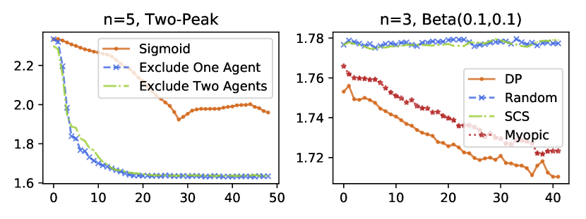
Figure 1: Effect of Distribution Info on Training

Figure 2 (Top-Left $n=3$, Top-Right $n=5$, Bottom-Left $n=10$) shows the performance comparison of supervision to different manual mechanisms. For $n=3$, supervision to DP performs the best. Random initializations is able to catch up but not completely close the gap. For $n=5$, random initializations caught up and actually became the best performing one. The Myopic curve first increases and then decreases because it needs to first fix the constraint violations. For $n=10$, supervision to DP significantly outperforms the others. Random initializations closes the gap with regard to serial cost sharing, but it then gets stuck. Even though it looks like the DP curve is flat, it is actually improving, albeit very slowly. A magnified version is shown in Figure 2 (Bottom-Right).

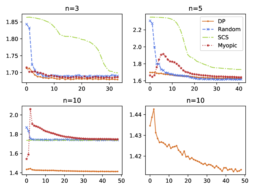
Figure 2: Supervision to Different Manual Mechanisms

Figure 3 shows two experiments on maximizing expected social welfare (y-axis) under two-peak $(0.2,0.1,0.6,0.1,0.5)$. For $n=3$, supervision to DP leads to the best result. For $n=5$, SCS is actually the best mechanism we can find (the cost function barely moves). It should be noted that all manual mechanisms before training have very similar welfares: $0.7517$ (DP), $0.7897$ (SCS), $0.7719$ (Myopic). Even random initialization before training has a welfare of $0.7648$. It could be that there is just little room for improvement here.

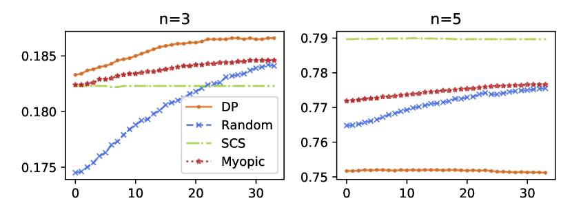
Figure 3: Maximizing Social Welfare

References

- [1] Mark Bagnoli and Ted Bergstrom. Log-concave probability and its applications. Economic Theory, 26(2):445–469, Aug 2005.
- [2] Vincent Conitzer and Tuomas Sandholm. Complexity of mechanism design. In Adnan Darwiche and Nir Friedman, editors, UAI ’02, Proceedings of the 18th Conference in Uncertainty in Artificial Intelligence, University of Alberta, Edmonton, Alberta, Canada, August 1-4, 2002, pages 103–110. Morgan Kaufmann, 2002.
- [3] Rajat Deb and Laura Razzolini. Voluntary cost sharing for an excludable public project. Mathematical Social Sciences, 37(2):123 – 138, 1999.
- [4] Paul Duetting, Zhe Feng, Harikrishna Narasimhan, David Parkes, and Sai Srivatsa Ravindranath. Optimal auctions through deep learning. In Kamalika Chaudhuri and Ruslan Salakhutdinov, editors, Proceedings of the 36th International Conference on Machine Learning, volume 97 of Proceedings of Machine Learning Research, pages 1706–1715, Long Beach, California, USA, 09–15 Jun 2019. PMLR.
- [5] Noah Golowich, Harikrishna Narasimhan, and David C. Parkes. Deep learning for multi-facility location mechanism design. In Proceedings of the Twenty-Seventh International Joint Conference on Artificial Intelligence, IJCAI-18, pages 261–267. International Joint Conferences on Artificial Intelligence Organization, 7 2018.
- [6] Mingyu Guo, Yong Yang, and Muhammad Ali Babar. Cost sharing security information with minimal release delay. In Tim Miller, Nir Oren, Yuko Sakurai, Itsuki Noda, Bastin Tony Roy Savarimuthu, and Tran Cao Son, editors, PRIMA 2018: Principles and Practice of Multi-Agent Systems, pages 177–193, Cham, 2018. Springer International Publishing.
- [7] Padala Manisha, C. V. Jawahar, and Sujit Gujar. Learning optimal redistribution mechanisms through neural networks. In Elisabeth André, Sven Koenig, Mehdi Dastani, and Gita Sukthankar, editors, Proceedings of the 17th International Conference on Autonomous Agents and MultiAgent Systems, AAMAS 2018, Stockholm, Sweden, July 10-15, 2018, pages 345–353. International Foundation for Autonomous Agents and Multiagent Systems Richland, SC, USA / ACM, 2018.
- [8] Andreu Mas-Colell, Michael Whinston, and Jerry R. Green. Microeconomic Theory. Oxford University Press, 1995.
- [9] J. Moore. General Equilibrium and Welfare Economics: An Introduction. Springer, 2006.
- [10] H. Moulin. Axioms of Cooperative Decision Making. Cambridge University Press, 1988.
- [11] Hervé Moulin. Serial cost-sharing of excludable public goods. The Review of Economic Studies, 61(2):305–325, 1994.
- [12] Shinji Ohseto. Characterizations of strategy-proof mechanisms for excludable versus nonexcludable public projects. Games and Economic Behavior, 32(1):51 – 66, 2000.
- [13] Adam Paszke, Sam Gross, Soumith Chintala, Gregory Chanan, Edward Yang, Zachary DeVito, Zeming Lin, Alban Desmaison, Luca Antiga, and Adam Lerer. Automatic differentiation in PyTorch. In NIPS Autodiff Workshop, 2017.
- [14] Ran Shao and Lin Zhou. Optimal allocation of an indivisible good. Games and Economic Behavior, 100:95 – 112, 2016.
- [15] Weiran Shen, Pingzhong Tang, and Song Zuo. Automated mechanism design via neural networks. In Proceedings of the 18th International Conference on Autonomous Agents and MultiAgent Systems, AAMAS ’19, pages 215–223, Richland, SC, 2019. International Foundation for Autonomous Agents and Multiagent Systems.
- [16] Joseph Sill. Monotonic networks. In Proceedings of the 1997 Conference on Advances in Neural Information Processing Systems 10, NIPS ’97, pages 661–667, Cambridge, MA, USA, 1998. MIT Press.
- [17] Makoto Yokoo. Characterization of strategy/false-name proof combinatorial auction protocols: Price-oriented, rationing-free protocol. In Proceedings of the 18th International Joint Conference on Artificial Intelligence, IJCAI’03, pages 733–739, San Francisco, CA, USA, 2003. Morgan Kaufmann Publishers Inc.
- [18] Zhi-Hua Zhou and Ji Feng. Deep forest: Towards an alternative to deep neural networks. In Proceedings of the 26th International Joint Conference on Artificial Intelligence, IJCAI’17, pages 3553–3559. AAAI Press, 2017.