The magnetized Vlasov-Ampère system and the Bernstein-Landau paradox

Abstract

We study the Bernstein-Landau paradox in the collisionless motion of an electrostatic plasma in the presence of a constant external magnetic field. The Bernstein-Landau paradox consists in that in the presence of the magnetic field, the electric field and the charge density fluctuation have an oscillatory behavior in time. This is radically different from Landau damping, in the case without magnetic field, where the electric field tends to zero for large times. We consider this problem from a new point of view. Instead of analyzing the linear magnetized Vlasov-Poisson system, as it is usually done, we study the linear magnetized Vlasov-Ampère system. We formulate the magnetized Vlasov-Ampère system as a Schrödinger equation with a selfadjoint magnetized Vlasov-Ampère operator in the Hilbert space of states with finite energy. The magnetized Vlasov-Ampère operator has a complete set of orthonormal eigenfunctions, that include the Bernstein modes. The expansion of the solution of the magnetized Vlasov-Ampère system in the eigenfunctions shows the oscillatory behavior in time. We prove the convergence of the expansion under optimal conditions, assuming only that the initial state has finite energy. This solves a problem that was recently posed in the literature. The Bernstein modes are not complete. To have a complete system it is necessary to add eigenfunctions that are associated with eigenvalues at all the integer multiples of the cyclotron frequency. These special plasma oscillations actually exist on their own, without the excitation of the other modes. In the limit when the magnetic fields goes to zero the spectrum of the magnetized Vlasov-Ampère operator changes drastically from pure point to absolutely continuous in the orthogonal complement to its kernel, due to a sharp change on its domain. This explains the Bernstein-Landau paradox. Furthermore, we present numerical simulations that illustrate the Bernstein-Landau paradox. In Appendix  B we provide exact formulas for a family of time-independent solutions.

1 Introduction

Collisionless motion of an electrostatic plasma can exhibit wave damping, a phenomenon identified by Landau in [18], and that is called Landau damping. It consists in the decay for large times of the electric field. There is a very extensive literature on Landau damping. See for example, [10, 11, 12, 27, 30, 31], and the references quoted there. For a recent deep mathematical study of Landau damping in the nonlinear case see [21]. On the contrary, it is known that magnetized plasmas can prevent Landau damping [6]. In fact, it was shown by Bernstein [6] that in the presence of a constant magnetic field the electric field does not decay for large times, and that, actually, it has an oscillatory behavior as a function of time. This phenomenon is called the Bernstein-Landau paradox, see for example [32], because it seems paradoxical that even an arbitrary small, but nonzero, value of the external constant magnetic field can be the cause of this radical change in the behaviour of the electric field for large times. The standard theory of the Bernstein-Landau paradox in the physics literature is based on the representation of the solutions to the magnetized Vlasov-Poisson system of equations in terms of a series of Bernstein modes. See, for example, [30][section 9.16] and [31][section 4.4.1].

It is the purpose of the present work to revisit the Bernstein-Landau paradox from a new point of view. Instead of considering the magnetized Vlasov-Poisson system we study the magnetized Vlasov-Ampère system. We write the magnetized Vlasov-Ampère system as a Schrödinger equation where the magnetized Vlasov-Ampère operator plays the role of the Hamiltonian. We construct a realization of the magnetized Vlasov-Ampère operator as a selfadjoint operator in the Hilbert space, that we call $\mathcal{H},$ that consists of the charge density functions that are square integrable and of the electric fields that are square integrable and of mean zero. Actually, the square of the norm of $\mathcal{H}$ is the energy. From the physical point of view this permits us to use the conservation of the energy in a very explicit way. On the mathematical side, this allows us to bring into the fore the powerful methods of the spectral theory of selfadjoint operators in a Hilbert space. There is a very extensive literature in spectral theory, see for example [15, 23, 24, 25, 26]. This approach has previously been used in the case without magnetic field to analyze the Landau-damping in [11, 12]. Within this framework the study of the Bernstein-Landau paradox reduces to the proof that the magnetized Vlasov-Ampère operator only has pure point spectrum, i.e., that its spectrum consists only of eigenvalues. Then, the fact that the magnetized Vlasov-Ampère operator has a complete set of orthonormal eigenfunctions follows from the abstract spectral theory of selfadjoint operators. We expand the general solutions to the magnetized Vlasov-Ampère system in the orthonormal basis of eigenfunctions of the magnetized Vlasov-Ampère operator. The coefficients of this expansion are the product of the scalar product of the initial state with the corresponding eigenfunction, and of the phase $e^{-it\lambda},$ where $t$ is time and $\lambda$ is the eigenvalue of the eigenfunction. This representation of the solution shows the oscillatory behavior in time for $\lambda\neq 0$, or constant in time for $\lambda=0,$ that is to say the Bernstein-Landau paradox. Moreover, our representation of the solution as an expansion in the orthonormal basis of eigenfunctions of the magnetized Vlasov-Ampère operator converges strongly in $\mathcal{H}$ for any initial data in $\mathcal{H},$ that is to say for any square integrable initial state without any further restriction in regularity and decay. Note that our result is optimal, since square integrability is the minimum that we can require, even to pose precisely the problem. A physical state has to have finite energy, i.e., it has to be square integrable.Note moreover, that we prove that the Bernstein modes are not complete. In fact, we prove in Theorem  6.3 that for general initial data with finite energy, and that satisfy the Gauss law, the charge density fluctuation is a sum of two terms. One of them is oscillatory in time (see (6.16)) and it coincides with the standard series of Bernstein modes given in [6, 5]. The other term, given in (6.15), is constant in time, and it is a series of eigenfunctions with eigenvalue zero, of the magnetized Vlasov-Ampére system, and that satisfy the Gauss law. It appears that the fact that the Bernstein modes are not enough to expand the general charge density fluctuation, and that one has also to consider static modes is a new result, that has not been observed previously in the literature. We prove that the spectrum of the magnetized Vlasov-Ampère operator is pure point in two different ways.

In the first one, we actually compute the eigenvalues and we explicitly construct a orthonormal basis of eigenfunctions, i.e., a complete set of orthonormal eigenfunctions. This, of course, gives us much more than just that the expansion of the charge density fluctuation, and is interesting in its own right, because it can be used for many other purposes. As we mentioned above, our analysis shows that the Bernstein modes alone are not a complete orthonormal system. In addition to the eigenfunctions with eigenvalue zero that contribute to the static part of the charge density fluctuation, to have a complete orthonormal system in the Hilbert space, $\mathcal{H}$ of configurations with finite energy, it is necessary to add other eigenfunctions that are associated with eigenvalues at all the integer multiples of the cyclotron frequency, including the zero eigenvalue. These other eigenfunctions have nontrivial density function, but the electric field and the charge density fluctuation are zero. Recall that the charge density fluctuation is obtained averaging the density function over the velocities. In consequence, these other eigenfunctions do not appear in the expansion of the charge density fluctuation. Anyhow, these eigenfunctions are physically interesting because they show that there are plasma oscillations such that at each point the charge density fluctuation and the electric field are zero. Some of them are time independent. Note that since our eigenfunctions are orthonormal, these special plasma oscillations actually exist on their own, without the excitation of the other modes. It appears to us that this fact, or at least the exact form of these eigenfunctions, with zero charge density fluctuation and zero electric field, has not been observed previously in the literature.

In the second one we use an abstract operator theoretical argument based on the celebrated Weyl theorem on the invariance of the essential spectrum of a selfadjoint operators in Hilbert space. This argument allows us to prove that the magnetized Vlasov-Ampère operator has pure point spectrum. It gives a less detailed information about where the eigenvalues are located, and it tells us nothing about the eigenfunctions. However, it is enough for the proof of the existence of the Bernstein-Landau paradox without going through the detailed calculations of the first approach. It also tells us why the Bernstein-Landau paradox exists from a general principle in spectral theory.

On the contrary in the case where the magnetic field is zero, it was proven in [11, 12] that the spectrum of the magnetized Vlasov-Ampère operator is made of an absolutely continuous part and of a kernel. The Landau damping follows from the well known fact that for a selfadjoint operator $\mathbf{H}$, the operator $e^{-it\mathbf{H}}P_{0}$ goes weakly to zero as $t\to\pm\infty$ (here $P_{0}$ is the projection on the absolutely continuous part of the spectrum). It has been remarked in [10] that there are ”interesting analogies with Lax and Phillips scattering theory ” [19]. In fact, the results of [11, 12] prove that it is not just an analogy, but the consequence of a convenient reformulation of Landau damping in terms of the magnetized Vlasov-Ampère system. The sharp change in the spectrum of the magnetized Vlasov-Ampère operator when the magnetic field goes to zero, i.e. from pure point to absolutely continuous in the orthogonal complement to its kernel, may appear to be paradoxical because the formal magnetized Vlasov-Ampère operator is formally analytic in the magnetic field. The issue is that the domain of the selfadjoint realization of the magnetized Vlasov-Ampère operator changes abruptly when the magnetic field is zero. It is a well known fact in the spectral theory of families of linear operators that the spectrum can change sharply at values of the parameter where the domain of the operator sharply changes. For a comprehensive presentation of these results the reader can consult, for example, [15]. Summing up, this shows that there is no paradox in the Bernstein-Landau paradox, just a well known fact of spectral theory, but, of course, in the physics literature the domains of the operators are usually not taken into account. Perhaps the reason why the absence of Landau damping for arbitrarily small magnetic fields is considered as paradoxical is related to the fact that the magnetized Vlasov-Poisson system somehow hides the underlying mathematical physics structure of our problem, in spite of the fact that it is a convenient tool, particularly for computational purposes. Let us explain what we mean. The full Maxwell equations consist of the Maxwell-Faraday equation, the Ampère equation, the Gauss law, and the Gauss law for magnetism, i.e., the divergence of the magnetic field is zero. In our case the Maxwell-Faraday equation and the Gauss law for magnetism are automatically satisfied. So, of the Vlasov-Maxwell equations, only the Vlasov equation remains, as well as the Ampère equation, and the Gauss law. Furthermore, the Gauss law is a constraint that is only necessary to impose at the initial time, since it is propagated by the magnetized Vlasov-Ampère system. Further, both the Vlasov and the Ampère equations are evolution equations. So, the natural way to proceed is to solve the magnetized Vlasov-Ampère system as an evolution problem, and to restrict the initial data to those who satisfy the Gauss law. The situation with the magnetized Vlasov-Poisson system is somewhat different because the Ampère equation is not explicitly taken into account. So, one could think that the magnetized Vlasov-Poisson system is incomplete. The remedy is that instead of imposing the Gauss law only at the initial time, it is required at all times. We actually prove in Section  2 that the magnetized Vlasov-Poisson system is indeed equivalent to the magnetized Vlasov-Ampère system plus the validity of the Gauss law at the initial time. However, the magnetized Vlasov-Poisson system is a hybrid one where the Vlasov equation is an evolution equation and the Poisson equation is an elliptic equation, without time derivative. This is one way to understand why in the magnetized Vlasov-Poisson system the basic mathematical physics of our problem is not so apparent. On the contrary, as we mentioned above, the magnetized Vlasov-Ampère system is an evolution problem, that moreover, as we already mentioned, and as we explain in Section  2, has a conserved energy that is explicitly expressed in terms of the density function and the electric field that appear in the magnetized Vlasov-Ampère system. These two facts are the reasons why the magnetized Vlasov-Ampère system has a selfadjoint formulation in Hilbert space, and then, it is clear that there is no paradox in the Bernstein-Landau paradox, as we explained above.

Once the selfadjointness of the magnetized Vlasov-Ampère formulation is established, it is a matter of explicit calculations to determine the eigenfunctions. The technicalities of the calculations are related to the fact that three different natural decomposition are combined. The first one is based on Fourier decomposition (factors $e^{inx}$), the second one is based on a direct sum of the kernel of the operator and its orthogonal (it will be denoted as $\mathcal{H}=\mbox{Ker}[\mathbf{H}]\oplus\mbox{Ker}[\mathbf{H}]^{\perp}$) and the third one starts from the determination of the eigenfunctions with a vanishing electric field (it will be denoted as $F=0$). The combination of these three decompositions is made compatible with convenient notations.

Passing to the limit $\omega_{c}\to 0$ in the representation formulae is possible in principle. This requires a careful analysis. We do not consider this problem in this work except in the very last remark in Appendix  B. Nevertheless, in Lemma 5.3 two consecutive eigenvalues are different by the constant $\omega_{c}$ and in Lemma 5.6 two consecutive eigenvalues are different by a value that is smaller than $2\,\omega_{c}$. Therefore, at the limit $\omega_{c}\to 0$, the discrete spectrum fills the entire real line with density and so it approaches the spectrum of the limit problem without magnetic field. A recent mathematical work [5] studied the Vlasov and the Vlasov-Fokker-Planck equations in a box, in three dimensions in configuration and in velocity space, and with a constant background magnetic field. They consider the Landau damping, the Bernstein-Landau paradox and the enhanced collisional relaxation in the limit when the collision frequency goes to zero. Since in this paper we study the case when there are no collisions, we will only comment on the results of [5] when the collision frequency is zero. We denote by $\mathcal{T}^{3}$ the three-dimensional torus, ie., $\mathcal{T}^{3}:=[0,2\pi]^{3}_{\rm per}.$ In the collisionless case [5] considers the following linearized magnetized Vlasov-Poisson system for $(\mathbf{x},\mathbf{v})\in\mathcal{T}^{3}\times\mathbb{R}^{3}$, where $\mathbf{x}=(x,y,z),$ and $\mathbf{v}=(v_{1},v_{2},v_{3}),$

$$\left\{\begin{aligned} &\partial_{t}\mathcal{G}(t,\mathbf{x},\mathbf{v})+\mathbf{v}\cdot\nabla_{\mathbf{x}}\mathcal{G}(t,\mathbf{x},\mathbf{v})+\frac{q}{m}\mathcal{F}(t,\mathbf{x})\cdot\nabla_{\mathbf{v}}{f^{0}(\mathbf{v})}+\frac{q}{m}\mathbf{v}\times\mathbf{B}_{0}\cdot\nabla_{\mathbf{v}}\mathcal{G}(t,\mathbf{x},\mathbf{v})=0,\qquad\mathcal{G}(0,\mathbf{x},\mathbf{v})=\mathcal{G}_{\rm in}(\mathbf{x},\mathbf{v}),\\ &\mathcal{F}(t,\mathbf{x})=-\nabla_{\mathbf{x}}\,\int_{\mathcal{T}^{3}}\,W(\mathbf{x}-\mathbf{y})\,\rho(t,\mathbf{y})\,d^{3}\mathbf{y},\\ &\int_{\mathcal{T}^{3}\times\mathbb{R}^{3}}\,\mathcal{G}(t,\mathbf{x},\mathbf{v})\,d^{3}\mathbf{x}\,d^{3}\mathbf{v}=0,\end{aligned}\right.$$ (1.1)

where,

$$\rho(t,\mathbf{x}):=\int_{\mathbb{R}^{3}}\,\mathcal{G}(t,\mathbf{x},\mathbf{v})\,d^{3}\mathbf{v},$$

and

$$W(\mathbf{x}):=\frac{q}{4\pi}\,\frac{1}{(2\pi)^{3}}\,\sum_{\mathbf{k}\in\mathbb{Z}^{3}\setminus\{0\}}\,\frac{1}{|\mathbf{k}|^{2}}\,e^{ik\cdot\mathbf{x}},$$

$q,m>0,$ and $\mathbf{B}_{0}=(0,0,B_{0}),B_{0}>0.$ Moreover,

$$f^{0}(v)=\frac{1}{2\pi}\,e^{-\frac{v_{1}^{2}+v_{2}^{2}}{2}}\,\left(\frac{1}{\sqrt{2\pi T_{\parallel}}}\,e^{-\frac{-v_{3}^{2}}{2T_{\parallel}}}+\tilde{f}(v_{3}^{2})\right),$$ (1.2)

with $T_{\parallel}>0.$

To state the results of [5] we first introduce some notation. Let us define the Fourier coefficients of $f\in L^{2}(\mathcal{T}^{3})$ as follows,

$$\hat{f}(\mathbf{k}):=\int_{\mathcal{T}^{3}}\,e^{-i\mathbf{k}\cdot\mathbf{x}}\,f(\mathbf{x})\,d^{3}\mathbf{x},\qquad\mathbf{k}=(k_{1},k_{2},k_{3})\in\mathbb{Z}^{3}.$$

Then,

$$f(\mathbf{x})=\frac{1}{(2\pi)^{3}}\,\sum_{\mathbf{k}\in\mathbb{Z}^{3}}\,e^{i\mathbf{k}\cdot\mathbf{x}}\,\hat{f}(\mathbf{k}).$$

Denoting $<\mathbf{v}>:=\sqrt{1+|\mathbf{v}|^{2}},$ the $H^{\sigma}_{m}$ norm of a function f is defined as follows [5],

$$\|f\|^{2}_{H^{\sigma}_{m}}:=\int_{\mathcal{T}^{3}\times\mathbb{R}^{3}}\,<\mathbf{v}>^{2m}|<\nabla>^{\sigma}\,f(\mathbf{x},\mathbf{v})|^{2}\,d^{3}\mathbf{x}d^{3}\mathbf{v},$$

with $\nabla=\nabla_{\mathbf{x},\mathbf{v}}$ the differential operator both in $\mathbf{x}$ and $\mathbf{v}.$

In [5] the following theorem is stated.

THEOREM 1.1.

(Bedrossian and Wang, Theorem 1, [5]) Let $<\mathbf{v}>^{m}\mathcal{G}_{\rm in}\in H^{\sigma},$ for $\sigma\geq 0,$ and $m>2.$ Suppose that $\|\tilde{f}\|_{H^{\sigma^{\prime}}_{m}}\leq\delta_{0},$ with $\sigma^{\prime}>\sigma+5/2,$ and $|T_{\parallel}-1|+\delta_{0}$ sufficient small depending on universal constants and $B_{0}$. Then, the following holds.

• The Landau damping for $z-$dependent modes:

  $$\||\partial_{z}|^{1/2}<\nabla,\partial_{z}t>^{\sigma}\rho(t)\|_{L^{2}_{t}L^{2}_{x}}\lesssim_{\sigma,\sigma^{\prime},m}\,\|\mathcal{G}_{\rm in}\|_{H^{\sigma}_{m}}.$$

• If $k_{3}=0,$and we additionally have $\sigma>5/2,$ then for all $\mathbf{k}_{\perp}:=(k_{1},k_{2},0)$ and $n\in\mathbb{N},$ $\exists!$ $b_{n,\mathbf{k}}=b_{n,\mathbf{k}}(\frac{q}{m}B_{0})\in(n,n+1)$ and coefficients $r_{\pm n,\mathbf{k}}$ depending on $\mathcal{G}_{\rm in}$ such that (with the convention that $r_{-0,\mathbf{k}}$ is distinct from $r_{0,\mathbf{k}}),$

  $$\hat{\rho}(t,\mathbf{k}_{\perp},0)=\sum_{n=0}^{\infty}\,r_{n,\mathbf{k}}\,e^{i\frac{b_{n,\mathbf{k}}qB_{0}}{m}t}+r_{-n,\mathbf{k}}\,e^{-i\frac{b_{n,\mathbf{k}}qB_{0}}{m}t},$$ (1.3)

  and further, there holds,

  $$\left|r_{\pm n,\mathbf{k}}\right|\leq\frac{1}{<\mathbf{k}>^{\alpha}\,<n>^{\gamma}}\,\|\mathcal{G}_{\rm in}\|_{H^{\sigma}_{m}},$$

  where $\alpha,\beta,\gamma$ are such that $\gamma=\min(\beta+1,2\beta-1),\alpha+2\beta-\frac{1}{2}\leq\sigma,$ and $\beta+1<m.$

Item a) of Theorem 1 of [5] (Theorem 1.1 above) is concerned with the Landau damping of the $z-$dependent modes (see also [6]), that is to say, of the modes that depend on the coordinate, $z,$ along the direction of the magnetic field $\mathbf{B}_{0}$. In this work we do not consider this problem, since as we work in $1+2$ dimensions our modes only depend on the coordinate $x$ that is orthogonal to the direction of the magnetic field $\mathbf{B}_{0}.$

Item b) of Theorem 1 of [5] (Theorem 1.1 above) considers the expansion of the Fourier coefficients, $\hat{\rho}(t,k_{\perp},0)$ of the charge density fluctuation in terms of the Bernstein modes, that is to say the Bernstein-Landau paradox, in the case of $3+3$ dimensions. This is the problem that we consider in $1+2$ dimensions in this work. We now proceed to discuss this result. Let us first show that if $\hat{\rho}(t,k_{\perp},0)$ in (1.3) is time independent, then it has to be identically zero. Assume then, that $\hat{\rho}(t,\mathbf{k}_{\perp},0)=\hat{\rho}(\mathbf{k}_{\perp},0).$ Since all the $b_{n,\mathbf{k}}$ are different from each other, and different from zero, then one deduces

$$\begin{array}[]{lll}0&=&\lim_{T\to\infty}\,\int_{0}^{T}\,\hat{\rho}(\mathbf{k}_{\perp},0)\,e^{\mp i\frac{b_{j,\mathbf{k}}qB_{0}}{m}t}\,dt\\ &=&\lim_{T\to\infty}\,\int_{0}^{T}\,\left(\sum_{n=0}^{\infty}\,r_{n,\mathbf{k}}\,e^{i\frac{b_{n,\mathbf{k}}qB_{0}}{m}t}+r_{-n,\mathbf{k}}\,e^{-i\frac{b_{n,\mathbf{k}}qB_{0}}{m}t}\right)e^{\mp i\frac{b_{j,\mathbf{k}}qB_{0}}{m}t}\,dt\\ &=&r_{\pm j,\mathbf{k}}.\end{array}$$ (1.4)

Hence, $r_{\pm n,\mathbf{k}}=0$ for all $n\in\mathbb{N},$ and all $\mathbf{k}=(\mathbf{k}_{\perp},0).$ Therefore, item b) of Theorem 1 of [5] (Theorem 1.1 above) implies that for the time independent solutions to (1.1) the Fourier coefficient of the charge density, $\hat{\rho}(\mathbf{k}_{\perp}0),$ is identically zero for all $\mathbf{k}_{\perp}.$ Recall that $\hat{\rho}(\mathbf{k})$ is the Fourier coefficient of $\rho(\mathbf{x}),$ that is to say,

$$\hat{\rho}(\mathbf{k}):=\int_{\mathcal{T}^{3}}\,\rho(\mathbf{x})\,e^{-i\mathbf{k}\mathbf{x}}d\mathbf{x}.$$

Then, inverting the Fourier series,

$$\rho(\mathbf{x})=\frac{1}{(2\pi)^{3}}\,\sum_{\mathbf{k}\in\mathbb{Z}^{3}}\,e^{i\mathbf{k}\mathbf{x}}\,\hat{\rho}(\mathbf{k}).$$ (1.5)

Further, by (1.5)

$$\int_{\mathcal{T}}\,\rho(x,y,z)\,dz=\frac{1}{(2\pi)^{2}}\,\sum_{(k_{1},k_{2})\in\mathbb{Z}^{2}}\,\,e^{i(k_{1}x+k_{2}y)}\,\hat{\rho}(k_{1},k_{2},0).$$

Hence, as for time independent solutions, if (1.3) holds, $\hat{\rho}(\mathbf{k}_{\perp},0)=0,$ we have proven that for the solutions given in Item b) of Theorem 1 of [5] (Theorem 1.1 above), if their are time independent, necessarily

$$\int_{\mathcal{T}}\,\rho(x_{\perp},x_{3})\,dx_{3}=0.$$ (1.6)

However, in Appendix  B we construct an explicit family of time-independent solutions to (1.1), that satisfy the hypotheses of item b) of Theorem 1 of [5] (Theorem 1.1 above) with $\hat{\rho}(k_{\perp},0)$ that is not identically zero, and where (1.6) does not holds. This shows that the result of item b) of Theorem 1 of [5] (Theorem 1.1 above) is devoted to the behaviour of a special class of solutions. This is clear by comparison with the physical literature [4, 6, 32] which is based on the study of a dispersion relation. The dispersion relation is mathematically justified in [5], in particular with a summability argument of the contributions of all poles of the dispersion relation. Nevertheless the pole $1/z$, that corresponds to time-independent solutions, is discarded in equation (2.14) in [5], and in this sense, the works [4, 6, 5] focus on a subclass, or special class, of solutions. In our work, we do not make such hypothesis or restriction and that is why we recover a time-independent solution as in [32, eq. (55)]. Note that in Appendix  B we write the model for ions, as in [5], for the purpose of making the comparison with the results of [5] more transparent. In the rest of our paper we write the model for electrons. Actually, the models for ions and electrons are the same, up to a change in the sign of the cyclotron frequency and of the electric field. See Remark 2.1. This is actually in agreement with our theoretical expansions in (6.14)-(6.16) that show that in general the charge density fluctuations have a time-independent part and a time-dependent part. Further, our result in (6.14)-(6.16) solves, in the case of one dimension in space and two dimensions in velocity, the problem posed in Remark 3 of [5] of justifying the expansion in the Bernstein modes of the charge density fluctuation, without the regularity in space and decay in velocity that they assume in Theorem 1 of [5] (Theorem 1.1 above). Our model is one dimensional in space and two dimensional in velocity. However, there is no difficulty to write it in three dimensions in space and velocity, because Maxwellian functions have a natural compatibility with separation of variables techniques. In principle, the extension of our results to three dimensions in space and velocity is possible with due attention paid to the anisotropy introduced by the magnetic field. It is left for further research.

The organization of this work is as follows. In Section 2 we introduce the magnetized Vlasov-Poisson and the magnetized Vlasov-Ampère systems, and we prove their equivalence. In Section 3 we give the notations and definitions that we use. In sections 4 we consider the case of a pure magnetized Vlasov equation without coupling. We construct a selfadjoint realization of the magnetized Vlasov operator, we explicitly compute the eigenvalues and we explicitly construct an orthonormal system of eigenfunctions that is complete, i.e., it is a basis of the Hilbert space. In Section 5 we construct a selfadjoint realization of the magnetized Vlasov-Ampère operator, we compute the eigenvalues, and we construct an orthonormal systems of eigenfunctions that is complete, that is to say that is a basis of the Hilbert space. In Section 6 we obtain a representation of the general solution to the magnetized Vlasov-Ampère system as an expansion in our orthonormal basis of eigenfunctions. In particular we prove the convergence of the Bernstein expansion [6], [5], under optimal conditions on the initial state. In Section 7 we give a operator theoretical proof of the existence of the Bernstein-Landau paradox, with an argument based on the Weyl theorem for the invariance of the essential spectrum. In Section 8 we illustrate our results with numerical calculations. In Appendix A we study the properties of the secular equation. Finally, in Appendix  B we construct explicit families of time-independent solutions to the linearized magnetized Vlasov-Poisson system.

2 The magnetized Vlasov-Poisson and the magnetized Vlasov-Ampère systems

We adopt the Klimontovitch approach [16, 14] where the Newton equation of a very large number of charged particles with velocity $v$ moving in an electromagnetic field is approximated by a continuous density function $f(t,x,v)\geq 0.$ The variable $t$ is time. We assume that the charged particles undergo a one dimensional motion, and that the real variable $x$ is the position of the charged particles. Furthermore, we suppose that the velocity, $v,$ of the charged particles is two dimensional, i.e., $v=(v_{1},v_{2})\in\mathbb{R}^{2}.$ Further, we take the motion of the charged particles along the first coordinate axis of the velocity of the charged particles. The density function is a solution of a Vlasov equation,

$$\partial_{t}f+v_{1}\partial_{x}f+\mathbf{F}\cdot\nabla_{v}f=0.$$ (2.1)

We assume, for simplicity, that the motion of the charged particles is a $2\pi$-periodic oscillation, that is a usual assumption [10]. Hence, we look for solutions to (2.1), $f(t,x,v),$ for $t\in\mathbb{R},x\in[0,2\pi],v=(v_{1},v_{2})\in\mathbb{R}^{2},$ that are periodic in $x,$ i.e., $f(t,0,v)=f(t,2\pi,v).$ The electromagnetic Lorentz force,

$$\mathbf{F}(t,x)=\frac{q}{m}\left(\mathbf{E}(t,x)+v\times\mathbf{B}(t,\mathbf{x})\right),$$ (2.2)

is divergence free with respect to the velocity variable, that is $\nabla_{v}\cdot\mathbf{F}=0$. The Maxwell’s equations are simplified, assuming that the magnetic field $\mathbf{B}(t,\mathbf{x})=\mathbf{B}_{0}$ is constant in space-time. Following the convention adopted in [4, 32], we suppose that the two dimensional velocity $v$ is perpendicular to the constant magnetic field, i.e., $\mathbf{B}_{0}=(0,0,B_{0}),B_{0}>0.$ Moreover, we assume that the electric field is directed along the first coordinate axis, $\mathbf{E}(t,x)=(E(t,x),0,0).$ We adopt a convenient normalization adapted to electrons, that is $q_{\rm ref}=-1$ and $m_{\rm ref}=1,$ where $q_{\rm ref}$ is the charge of the electron, and $m_{\rm ref}$ is the mass of the electron. The electric field satisfies the Gauss law,

$$\partial_{x}E(t,x)=2\pi-\int_{\mathbb{R}^{2}}\,fdv,$$ (2.3)

where $2\pi$ is the constant density of the heavy ions, that do not move. We take the density of the ions equal to $2\pi$ to simplify some of the calculations below. The term $-\int_{\mathbb{R}^{2}}\,f\,dv$ is the charge density of the particles with charge $-1.$

With these notations and normalizations (2.1), and (2.3) are written as the following system,

$$\left\{\begin{aligned} &\partial_{t}f+v_{1}\partial_{x}f-E\partial_{v_{1}}f+\omega_{c}\left(-v_{2}\partial_{v_{1}}+v_{1}\partial_{v_{2}}\right)f=0,\\ &\partial_{x}E(t,x)=2\pi-\int_{\mathbb{R}^{2}}\,fdv.\end{aligned}\right.$$ (2.4)

We denote the cyclotron frequency by $\omega_{\text{\rm{c}}}:=B_{0}$.

REMARK 2.1.

The model written for positive ions instead of (negatively charged) electrons is similar to (2.4), with the only modification that the sign in front of the electric field and $\omega_{c}$ is changed in both equations.

We retain the potential part of the electric field

$$E(t,x)=-\partial_{x}\varphi(t,x),$$ (2.5)

where the potential $\varphi(t,\mathbf{x})$ is a solution to the Poison equation,

$$\quad-\Delta\varphi=2\pi-\int_{\mathbb{R}^{2}}\,fdv.$$ (2.6)

The electric field and the potential are assumed to be periodic with period $2\pi,$ i.e. $E(t,0)=E(t,2\pi),\varphi(t,0)=\varphi(t,2\pi).$ Note that since the potential $\varphi(t,x)$ is periodic it follows from (2.5) that the mean value of the electric field is zero,

$$\int_{0}^{2\pi}\,E(t,x)\,dx=0.$$ (2.7)

Two important properties of the magnetized Vlasov-Poisson system (2.4, (2.5), and (2.6) are that the density function satisfies the maximum principle

$$\inf_{(x,v)\in[0,2\pi]\times\mathbb{R}^{2}}f_{\rm ini}(x,v)\leq f(t,x,v)\leq\sup_{(x,v)\in[0,2\pi]\times\mathbb{R}^{2}}f_{\rm ini}(x,v),$$

where $f_{\rm ini}$ is the initial value of the solution, $f(t,x,v),$ and that the total energy is constant in time,

$$\frac{d}{dt}\left(\int_{[0,2\pi]\times\mathbb{R}^{2}}\frac{|v|^{2}}{2}fdxdv+\int_{[0,2\pi]}\frac{|E|^{2}}{2}dx\right)=0.$$ (2.8)

Following [6], a linearization of the equations around a homogeneous Maxwellian equilibrium state $f_{0}(v),$ where, $f_{0}(v):=e^{\frac{-v^{2}}{2}}$ is performed. Here the Maxwellian distribution is normalized for $T_{\rm ref}\,k_{\rm B}=1,$ where $T_{\rm ref}$ is the reference temperature and $k_{\rm B}$ is Boltzmann’s constant. It corresponds to the expansion

$$f(t,x,v)=f_{0}(v)+\varepsilon\sqrt{f_{0}(v)}u(t,x,v)+O(\varepsilon^{2}),$$ (2.9)

and

$$E(t,x)=E_{0}+\varepsilon F(t,x)+O(\varepsilon^{2}),$$ (2.10)

with a null reference electric field $E_{0}=0$. Inserting (2.9) and (2.10) into (2.4), and keeping the terms up to linear in $\varepsilon,$ one gets the linearized magnetized Vlasov-Poisson system written as,

$$\left\{\begin{aligned} &\partial_{t}u+v_{1}\partial_{x}u+Fv_{1}\sqrt{f_{0}}+\omega_{c}\left(-v_{2}\partial_{v_{1}}+v_{1}\partial_{v_{2}}\right)u=0,\\ &\partial_{x}F=-\int_{\mathbb{R}^{2}}u\sqrt{f_{0}}dv,\\ &\int_{[0,2\pi]}F=0,\end{aligned}\right.$$ (2.11)

where in the third equation we have added the constraint that the mean value of the electric field $F$ is zero, as in (2.7). Moreover, the electric field $F(t,x)=-\partial_{x}\varphi(t,x)$ is obtained from a potential as in (2.5), where the potential is periodic, $\varphi(t,0)=\varphi(t,2\pi),$ and it solves the Poisson equation,

$$\quad-\Delta\varphi=-\int_{\mathbb{R}^{2}}\,u\,\sqrt{f_{0}}dv.$$ (2.12)

Observe that the second equation in (2.11) is the Gauss law,

$$\partial_{x}F(t,x)=\rho(t,x),$$ (2.13)

where $\rho(t,x)$ is the charge density fluctuation of the perturbation of the Maxwellian equilibrium state,

$$\rho(t,x):=-\int_{\mathbb{R}^{2}}\,u(t,x,v)\,\sqrt{f_{0}}(v)dv.$$ (2.14)

The study of the solutions to the magnetized Vlasov-Poisson system is the standard method to analyze the dynamics of a very large number of charged particles moving in the presence of a constant external magnetic field. For the case of the Bernstein-Landau paradox see, for example, [6], [32], [30][section 9.16], [31][[section 4.4.1] and [5]. We now present an alternate method to study this problem. In the full Maxwell equations one of the equation is the Ampère equation

$$\partial_{t}F=\int_{\mathbb{R}^{2}}\,v_{1}\,u\,\sqrt{f_{0}}dv,$$ (2.15)

where we have taken the dielectric constant $\varepsilon_{0}=1.$ We consider here the following modified Ampère equation

$$\partial_{t}F=I^{\ast}\int_{\mathbb{R}^{2}}\,v_{1}\sqrt{f_{0}}\,u\,dv,$$ (2.16)

where $I^{\ast}$ is the space operator such that $I^{*}g=g-[g]$ and the mean value in space of a function $g$ is denoted by $[g]$, that is to say, $I^{\ast}g(x):=g(x)-\frac{1}{2\pi}\,\int_{0}^{2\pi}\,g(y)\,dy$. With this convention the magnetized Vlasov-Ampère system is written as follows,

$$\left\{\begin{aligned} &\partial_{t}u+v_{1}\partial_{x}u+Fv_{1}\sqrt{f_{0}}+\omega_{c}\left(-v_{2}\partial_{v_{1}}+v_{1}\partial_{v_{2}}\right)u=0,\\ &\partial_{t}F=I^{\ast}\int_{\mathbb{R}^{2}}\,v_{1}\,\sqrt{f_{0}}\,udv.\end{aligned}\right.$$ (2.17)

To the magne:tized Vlasov-Ampère system (2.17), we add conditions for $F_{\rm ini}:=F(0,\cdot)$ and $u_{\rm ini}=u(0,\cdot,\cdot)$ : the integral constraint,

$$\int_{0}^{2\pi}\,F_{\rm ini}\,dx=0,$$ (2.18)

is satisfied at initial time, and the Gauss law (2.13), (2.14) is also satisfied at the initial time,

$$\frac{d}{dx}F_{\rm ini}=-\int_{\mathbb{R}^{2}}u_{\rm ini}\sqrt{f_{0}}dv.$$ (2.19)

LEMMA 2.2.

The linearized magnetized Vlasov-Poisson system (2.11) is equivalent to the magnetized Vlasov-Ampère system (2.17) with initial conditions that satisfy (2.18), (2.19).

Proof.

Let $(u,F)$ be a solution the magnetized Vlasov-Ampère system (2.17) that satisfy (2.18), (2.19). It follows from the Ampère equation that

$$\partial_{t}\int_{0}^{2\pi}\,F(t,x)\,dx=\int_{0}^{2\pi}\,I^{\ast}\int_{\mathbb{R}^{2}}\,v_{1}\,\sqrt{f_{0}}\,u=0$$

and consequently the integral constraint (2.18) is propagated to all times. The Gauss law (2.19) is propagated also to all times by the magnetized Vlasov-Ampère system, as we proceed to prove. Multiplying the first equation in (2.17) by $\sqrt{f_{0}},$ integrating in $v$ over $\mathbb{R}^{2},$ using that $f_{0}$ is an even function of $|v|$ and using integration by parts, we prove the following continuity equation,

$$\partial_{t}\int_{\mathbb{R}^{2}}u\sqrt{f_{0}}dv+\partial_{x}\int_{\mathbb{R}^{2}}v_{1}u\sqrt{f_{0}}dv=0.$$ (2.20)

Deriving (2.16) with respect to $x$ we obtain, $0=\partial_{x}\left(\partial_{t}F-I^{*}\int_{\mathbb{R}^{2}}v_{1}u\sqrt{f_{0}}dv\right)=\partial_{x}\left(\partial_{t}F-\int_{\mathbb{R}^{2}}v_{1}u\sqrt{f_{0}}dv\right)$, because $\partial_{x}=\partial_{x}I^{*}$. Then, by (2.20)

$$0=\partial_{t}\left(\partial_{x}F+\int_{\mathbb{R}^{2}}\,u\,\sqrt{f_{0}}\,dv\right),$$

from which the Gauss law follows for all times. We have proven that a solution to the magnetized Vlasov-Ampère system (2.17) that satisfies the initial conditions (2.18), (2.19) solves the magnetized Vlasov-Poisson system (2.11).
On the contrary let $(u,F)$ be a solution to the magnetized Vlasov-Poisson system (2.11). Then by the second equation in (2.11) and (2.20),

$$0=\partial_{x}\partial_{t}F+\partial_{t}\int_{\mathbb{R}^{2}}u\sqrt{f_{0}}dv=\partial_{x}\left(\partial_{t}F-\int_{\mathbb{R}^{2}}v_{1}u\sqrt{f_{0}}dv\right).$$

So $\partial_{t}F=\int_{\mathbb{R}^{2}}v_{1}u\sqrt{f_{0}}dv+C(t)$, where $C(t)$ is constant in space. Then, $\partial_{t}I^{*}F=I^{*}\int_{\mathbb{R}^{2}}v_{1}u\sqrt{f_{0}}dv$. But $F$ has zero mean value, so $I^{*}F=F$, and it follows that the Ampère law in (2.16) holds. Hence, the magnetizedVlasov-Poisson system implies the magnetized Vlasov-Ampère system (2.17) and the initial conditions (2.18), (2.19). ∎

From now on we only consider the magnetized Vlasov-Ampère system (2.17) with conditions (2.18), (2.19). A fundamental energy relation is easily shown for solutions of the magnetized Vlasov-Ampère formulation (2.17)

$$\frac{d}{dt}\left(\int_{[0,2\pi]\times\mathbb{R}^{2}}\frac{u^{2}}{2}dxdv+\int_{[0,2\pi]}\frac{F^{2}}{2}dx\right)=0.$$ (2.21)

It is the counterpart of the energy identity (2.8), so the term $\int_{[0,2\pi]\times\mathbb{R}^{2}}\int_{\mathbf{v}}\frac{u^{2}}{2}dxdv$ is identified with the kinetic energy of the negatively charged particles, and the term $\int_{[0,2\pi]}\frac{F^{2}}{2}dx$ is the energy of the electric field. This identity is known since [17, 3]. As we show in the next sections, the identity (2.21) is the basis of our formulation of the magnetized Vlasov-Ampère system as a Schrödinger equation in Hilbert space, where magnetized the Vlasov-Ampère operator plays the role of the selfadjoint Hamiltonian.

3 Notations and Definitions

We will write the magnetized Vlasov-Ampère system as a Schrödinger equation with a selfadjoint Hamiltonian in an appropriate Hilbert space. We find it convenient to borrow some terminology from quantum mechanics. For this purpose, we first introduce some notations and definitions. We designate by $\mathbb{R}^{+}$ the positive real semi-axis, i.e., $\mathbb{R}^{+}:=(0,\infty),$ and by $\mathbb{R}^{2}$ the plane. The set of all integers is denoted by $\mathbb{Z}$ and the set of all nonzero integers by $\mathbb{Z}^{\ast}.$ The positive natural numbers are designated by $\mathbb{N}^{*}.$ By $\mathbb{C}$ we designate the complex numbers. We denote by $C$ a generic constant whose value does not have to be the same when it appears in different places. By $C^{\infty}([0,2\pi])$ we designate the set of all infinitely differentiable functions in $[0,2\pi],$ and by $C^{\infty}_{0}(\mathbb{R}^{2})$ we denote the set of all infinitely differentiable functions in $\mathbb{R}^{2}$ with compact support. Let $\mathcal{B}$ be a set of vectors in a Hilbert space, $\mathbb{H}.$ We denote by $\text{\rm Span}[\mathcal{B}]$ the closure in the strong convergence in $\mathbb{H}$ of all finite linear combinations of elements of $\mathcal{B},$ in other words,

$$\text{\rm Span}[\mathcal{B}]:=\text{\rm{closure}}\left\{\sum_{j=1}^{N}\alpha_{j}X_{j}:\alpha_{j}\in\mathbb{C},X_{j}\in\mathcal{B},N\in\mathbb{N}^{*}\right\}.$$

Let $\mathcal{M}$ be a subset of a Hilbert space $\mathbb{H}.$ We define the orthogonal complement of $\mathcal{M}$, in symbol, $\mathcal{M}^{\perp},$ as follows,

$$\mathcal{M}^{\perp}:=\{f\in\mathbb{H}:(f,u)_{\mathbb{H}}=0,\,\text{\rm{ for all}}\,u\in\mathcal{M}\}.$$

Let $\mathbb{H}$ be a Hilbert space, and let $\mathbb{H}_{j},j=1,\dots,N,2\leq N\leq\infty,$ be mutually orthogonal closed subspaces of $\mathbb{H}$, that is to say,

$$\mathbb{H}_{j}\subset\mathbb{H}_{m}^{\perp},\,\text{\rm{and} }\,\mathbb{H}_{m}\subset\mathbb{H}_{j}^{\perp},\qquad j\neq m,1\leq j,m\leq N.$$

Note that if $\mathbb{H}_{j}$ and $\mathbb{H}_{m}$ are mutually orthogonal, then one has $(f,u)_{\mathbb{H}}=0$, $f\in\mathbb{H}_{j}$, $u\in\mathbb{H}_{m}$. We say that $\mathbb{H}$ is the direct sum of the $\mathbb{H}_{j},j=1,\dots,N,2\leq N\leq\infty,$ mutually orthogonal closed subspaces of $\mathbb{H}$, and we write,

$$\mathbb{H}=\oplus_{j=1}^{N}\,\mathbb{H}_{j},$$

if for any $f\in\mathbb{H},$ there are $f_{j}\in\mathbb{H}_{j},j=1,\dots,N,$ such that, $f=\sum_{j=1}^{N}\,f_{j}$. Note that the $f_{j},j=1,\dots,N$ are unique for a given $f,$ and that $\|f\|^{2}_{\mathbb{H}}=\sum_{j=1}^{N}\,\|f_{j}\|^{2}_{\mathbb{H}}$.

Let $A$ be an operator in a Hilbert space $\mathbb{H}$, and let us denote by $D[A]$ the domain of $A$. We say that the operator $B$ is an extension of the operator $A,$ in symbol, $A\subset B,$ if $D[A]\subset D[B],$ and if $Au=Bu,$ for all $u\in D[A].$ Suppose that the domain of $A$ is dense in $\mathbb{H}.$ We denote by $A^{\dagger}$ the adjoint of $A$, that is defined as follows,

$$D[A^{\dagger}]:=\{v\in\mathbb{H}:(Au,v)_{\mathbb{H}}=(u,f)_{\mathbb{H}},\text{\rm for some}\,f\in\mathbb{H},\text{\rm and for all}\,u\in D[A]\},$$

and

$$A^{\dagger}v=f,\qquad v\in D[A^{\dagger}].$$

We say that $A$ is symmetric if $A\subset A^{\dagger},$ and that $A$ is selfadjoint if $A=A^{\dagger},$ that is to say if $D[A]=D[A^{\dagger}],$ and $Au=A^{\dagger}u,u\in D[A]=D[A^{\dagger}].$ An essentially selfadjoint operator has only one selfadjoint extension. For any operator $A$ we denote by $\text{\rm Ker}[A]:=\{u\in D[A]:Au=0\}$ the set of all eigenvectors of $A$ with eigenvalue zero. For more information on the theory of operators in Hilbert space the reader can consult [15] and [23].

We denote by $L^{2}(0,2\pi)$ the standard Hilbert space of functions that are square integrable in $(0,2\pi).$ Furthermore, we designate by $L^{2}_{\text{\rm 0}}(0,2\pi)$ the closed subspace of $L^{2}(0,2\pi)$ consisting of all functions with zero mean value, i.e.,

$$L^{2}_{\text{\rm 0}}(2,\pi):=\left\{F\in L^{2}(0,2\pi):\int_{0}^{2\pi}\,F(x)\,dx=0\right\}.$$ (3.1)

Note that since all the functions in $L^{2}(0,2\pi)$ are integrable over $(0,2\pi)$ the space $L^{2}_{\text{\rm 0}}(0,2\pi)$ is well defined. Further, we denote by $L^{2}(\mathbb{R}^{2})$ the standard Hilbert space of all functions that are square integrable in $\mathbb{R}^{2}.$ Let us denote by $\mathcal{A}$ the tensor product of $L^{2}(0,2\pi)$ and of $L^{2}(\mathbb{R}^{2}),$ namely,

$$\mathcal{A}:=L^{2}(0,2\pi)\otimes L^{2}(\mathbb{R}^{2}).$$ (3.2)

For the definition and the properties of tensor products of Hilbert spaces the reader can consult Section 4 of Chapter II of [23]. We often make use of the fact that the tensor product of an orthonormal basis in $L^{2}(0,2\pi)$ and an orthonormal basis in $L^{2}(\mathbb{R}^{2})$ is an orthonormal basis in $\mathcal{A}.$ As shown in Section 4 of Chapter II of [23], the space $\mathcal{A}$ can be identified with the standard Hilbert space $L^{2}((0,2\pi)\times\mathbb{R}^{2})$ of square integrable functions in $(0,2\pi)\times\mathbb{R}^{2}$ with the scalar product,

$$\left(u,f\right)_{L^{2}((0,2\pi)\times\mathbb{R}^{2})}:=\int_{(0,2\pi)\times\mathbb{R}^{2}}\,u(x,v)\,\overline{f(x,v)}\,dx\,dv,$$

where $x\in(0,2\pi)$ and $v=(v_{1},v_{2})\in\mathbb{R}^{2}.$ Our space of physical states, that we denote by $\mathcal{H},$ is defined as the direct sum of $\mathcal{A}$ and $L^{2}_{0}(0,2\pi).$

$$\mathcal{H}:=\mathcal{A}\oplus L^{2}_{0}(0,2\pi).$$ (3.3)

We find it convenient to write $\mathcal{H}$ as the space of the column vector-valued functions, $\begin{pmatrix}u\\ F\end{pmatrix}$ where $u(x,v)\in\mathcal{A}$ and $F(x)\in L^{2}_{0}(0,2\pi).$ The scalar product in $\mathcal{H}$ is given by,

$$\left(\begin{pmatrix}u\\ F\end{pmatrix},\begin{pmatrix}f\\ G\end{pmatrix}\right)_{\mathcal{H}}:=(u,f)_{\mathcal{A}}+(F,G)_{L^{2}(0,2\pi)}.$$

Note that by the identity (2.21) the $\mathcal{H}$-norm of the solutions to the magnetized Vlasov-Ampère system is constant in time. This is the underlying reason why we will be able in later sections to formulate the magnetized Vlasov-Ampère system as a Schrödinger equation in $\mathcal{H}$ with a selfadjoint realization of the magnetized Vlasov-Ampère operator playing the role of the Hamiltonian. Moreover, the square of the norm of $\mathcal{H}$ is the constant energy of the solutions to the magnetized Vlasov-Ampère system.

Let us denote by $H^{(1)}(0,2\pi)$ the standard Sobolev space [2] of all functions in $L^{2}(0,2\pi)$ such that its derivative in the distribution sense is a function in $L^{2}(0,2\pi),$ with the scalar product,

$$(F,G)_{H^{(1)}(0,2\pi)}:=(F,G)_{L^{2}(0,2\pi)}+(\partial_{x}F,\partial_{x}G)_{L^{2}(0,2\pi)}.$$

We designate by $H^{(1,0)}(0,2\pi)$ the closed subspace of $H^{(1)}(0,2\pi)$ that consists of all functions in $F\in H^{(1)}(0,2\pi)$ such that $F(0)=F(2\pi)$ and that have mean zero. Namely,

$$H^{(1,0)}(0,2\pi):=\left\{F\in H^{(1)}(0,2\pi):F(0)=F(2\pi),\,\text{\rm and}\,\int_{0}^{2\pi}\,F(x)\,dx=0\right\}.$$

Note [2] that as the functions in $H^{(1)}(0,2\pi)$ have a continuous extension to $[0,2\pi],$ the space $H^{(1,0)}(0,2\pi)$ is well defined.

We denote by $L^{2}(\mathbb{R}^{+},rdr)$ the standard Hilbert space of functions defined on $\mathbb{R}^{+}$ with the scalar product,

$$(\tau,\eta)_{L^{2}(\mathbb{R}^{+},rdr)}:=\int_{0}^{\infty}\,\tau(r)\,\overline{\eta(r)}\,r\,dr.$$

4 The magnetized Vlasov equation without coupling

In this section we consider the case without electric field, i.e. the magnetized Vlasov equation. The results of this section will be useful in the study of the full magnetized Vlasov-Ampère system, that we carry over in Sections 5.

The magnetized Vlasov equation can be written as the following Schrödinger equation in $\mathcal{A},$

$$i\partial_{t}u=i\left(-v_{1}\partial_{x}+\omega_{\text{\rm c}}(v_{2}\,\partial_{v_{1}}-v_{1}\,\partial_{v_{2}})\right)u.$$ (4.1)

In the following proposition we obtain a complete orthonormal system of eigenfunctions for the magnetized Vlasov equation (4.1). To this end, we introduce the polar coordinates $(r,\varphi)$ of the velocity $v\in\mathbb{R}^{2}$.

PROPOSITION 4.1.

Let $\{\tau_{j}\}_{j=1}^{\infty}$ be an orthonormal basis of $L^{2}(\mathbb{R}^{+},rdr).$ Let $\varphi\in[0,2\pi),r>0,$ be polar coordinates in $\mathbb{R}^{2},v_{1}=r\cos\varphi,v_{2}=r\sin\varphi.$ For $(n,m,j)\in\mathbb{Z}^{2}\times\mathbb{N}^{*}$ we define,

$$u_{n,m,j}:=\frac{e^{in(x-\frac{v_{2}}{\omega_{\text{\rm c}}})}}{\sqrt{2\pi}}\,\frac{e^{im\varphi}}{\sqrt{2\pi}}\,\tau_{j}(r).$$ (4.2)

Then, the $u_{n,m,j},(n,m,j)\in\mathbb{Z}^{2}\times\mathbb{N}^{*}$ are an orthonormal basis in $\mathcal{A}.$ Furthermore, each $u_{n,m,j}$ is an eigenfunction for the magnetized Vlasov equation (4.1) with eigenvalue $\lambda^{(0)}_{m}=m\,\omega_{\text{\rm c}},$

$$i\left(-v_{1}\partial_{x}+\omega_{\text{\rm c}}(v_{2}\,\partial_{v_{1}}-v_{1}\,\partial_{v_{2}})\right)u_{n,m,j}=\,\lambda^{(0)}_{m}\,u_{n,m,j},\qquad(n,m,j)\in\mathbb{Z}^{2}\times\mathbb{N}^{*}.$$ (4.3)

Moreover, the eigenvalues $\lambda^{(0)}_{m},m\in\mathbb{Z},$ have infinite multiplicity.

Proof.

We first prove that the $u_{n,m,j},(n,m,j)\in\mathbb{Z}^{2}\times\mathbb{N}^{*}$ are an orthonormal basis in $\mathcal{A}.$ Clearly, it is an orthonormal system. To prove that it is a basis it is enough to prove that if a function in $\mathcal{A}$ is orthogonal to all the $u_{n,m,j},(n,m,j)\in\mathbb{Z}^{2}\times\mathbb{N}^{*},$ then, it is the zero function. Hence, assume that $u\in\mathcal{A}$ satisfies,

$$\left(u,u_{n,m,j}\right)_{\mathcal{A}}=0,\qquad(n,m,j)\in\mathbb{Z}^{2}\times\mathbb{N}^{*}.$$ (4.4)

Denote $g_{n}(v):=\int_{0}^{2\pi}\,e^{-inx}\,u(x,v)\,dx$. By the Cauchy-Schwarz inequality, one has $\left|g_{n}(v)\right|^{2}\leq 2\pi\int_{0}^{2\pi}\,|u(x,v)|^{2}\,dx$. Further, since $u\in\mathcal{A},$ it follows that $g_{n}\in L^{2}(\mathbb{R}^{2}).$ By (4.4), for each fixed $n\in\mathbb{Z},$

$$\int_{(0,2\pi)\times\mathbb{R}^{+}}\,g_{n}(v)\,e^{in\frac{v_{2}}{\omega_{\text{\rm c}}}}\,e^{-im\varphi}\,\overline{\tau_{j}(r)}\,d\varphi\,r\,dr=0,\qquad(m,j)\in\mathbb{Z}\times\mathbb{N}^{*}.$$

As the functions $\frac{1}{\sqrt{2\pi}}\,e^{im\varphi}\,\tau_{j}(r),m\in\mathbb{Z},j\in\mathbb{N}^{*}$ are an orthonormal basis in $L^{2}(\mathbb{R}^{2}),$ one has that $g_{n}(v)\,e^{in\frac{v_{2}}{\omega_{\text{\rm c}}}}=0$ for a.e. $v\in\mathbb{R}^{2}.$ Moreover, as $e^{in\frac{v_{2}}{\omega_{\text{\rm c}}}}$ is never zero, we obtain, $g_{n}(v)=0,$ for a.e. $v\in\mathbb{R}^{2},$ i.e., $\int_{0}^{2\pi}\,e^{-inx}\,u(x,v)\,dx=0,n\in\mathbb{Z}$. As the functions $\frac{1}{\sqrt{2\pi}}e^{inx},n\in\mathbb{Z}$ are an orthonormal basis in $L^{2}(0,2\pi)$, it follows that $u(x,v)=0.$ This completes the proof that the $u_{n,m,j},(n,m,j)\in\mathbb{Z}^{2}\times\mathbb{N}^{*},$ are an orthonormal basis of $\mathcal{A}.$ Equation (4.3) follows from a simple calculation using that $\partial_{v_{1}}=\frac{v_{1}}{r}\,\partial_{r}-\frac{v_{2}}{r^{2}}\,\partial_{\varphi},$ $\partial_{v_{2}}=\frac{v_{2}}{r}\,\partial_{r}+\frac{v_{1}}{r^{2}}\,\partial_{\varphi},$ and $v_{2}\,\partial_{v_{1}}-v_{1}\,\partial_{v_{2}}=-\partial_{\varphi}.$ Note that the eigenvalues $\lambda^{(0)}_{m}$ have infinite multiplicity because all the $u_{n,m,j}$ with $m$ fixed and $n\in\mathbb{Z},j\in\mathbb{N}^{*}$ are orthogonal eigenfunctions for $\lambda^{(0)}_{m}.$ ∎

Let us denote by $h_{0}$ the formal magnetized Vlasov operator with periodic boundary conditions in $x,$ that we define as follows,

$$h_{0}u:=i\left(-v_{1}\partial_{x}+\omega_{\text{\rm c}}(v_{2}\,\partial_{v_{1}}-v_{1}\,\partial_{v_{2}})\right)u,$$ (4.5)

with domain,

$$D[h_{0}]:=\mathcal{D},$$ (4.6)

where by $\mathcal{D}$ we denote the following space of test functions,

$$\mathcal{D}:=\{u\in C^{\infty}_{0}([0,2\pi]\times\mathbb{R}^{2}):\frac{d^{j}}{dx^{j}}u(0,v)=\frac{d^{j}}{dx^{j}}u(2\pi,v),j=1,\dots\},$$ (4.7)

where by $C^{\infty}_{0}([0,2\pi]\times\mathbb{R}^{2})$ we designate the space of all infinitely differentiable functions, defined in $[0,2\pi]\times\mathbb{R}^{2},$ and that have compact support in $[0,2\pi]\times\mathbb{R}^{2}.$

We will construct a selfadjoint extension of $h_{0}.$ For this purpose, we first introduce some definitions. Let us denote by $l^{2}(\mathbb{Z}^{2}\times\mathbb{N}^{*})$ the standard Hilbert space of square summable sequences, $s=\left\{s_{n,m,j},(n,m,j)\in\mathbb{Z}^{2}\times\mathbb{N}^{*}\right\}$ with the scalar product,

$$(s,d)_{l^{2}(\mathbb{Z}^{2}\times\mathbb{N}^{*})}:=\sum_{(n,m,j)\in\mathbb{Z}^{2}\times\mathbb{N}^{*}}\,s_{n,m,j}\,\overline{d_{n,m,j}}.$$

Let $\mathbf{U}$ be the following unitary operator from $\mathcal{A}$ onto $l^{2}(\mathbb{Z}^{2}\times\mathbb{N}^{*}),$

$$\mathbf{U}u:=\left\{(u,u_{n,m,j})_{\mathcal{A}},(n,m,j)\in\mathbb{Z}^{2}\times\mathbb{Z}\right\}.$$ (4.8)

We denote by $\widehat{H_{0}}$ the following operator in $l^{2}(\mathbb{Z}^{2}\times\mathbb{N}^{*}),$

$$\left\{(\widehat{H_{0}}\,s)_{n,m,j},(n,m,j)\in\mathbb{Z}^{2}\times\mathbb{N}^{*}\right\}:=\left\{\lambda^{(0)}_{m}s_{n,m,j},(n,m,j)\in\mathbb{Z}^{2}\times\mathbb{N}^{*}\right\},$$ (4.9)

with domain, $D[\widehat{H_{0}]},$ given by,

$$D[\widehat{H_{0}}]:=\left\{\left\{s_{n,m,j},(n,m,j)\in\mathbb{Z}^{2}\times\mathbb{N}^{*}\right\}\in l^{2}(\mathbb{Z}^{2}\times\mathbb{N}^{*}):\left\{\lambda^{(0)}_{m}\,s_{n,m,j},(n,m,j)\in\mathbb{Z}^{2}\times\mathbb{N}^{*}\right\}\in l^{2}(\mathbb{Z}^{2}\times\mathbb{N}^{*})\right\}.$$ (4.10)

The operator $\widehat{H_{0}}$ is selfadjoint because it is the multiplication operator by the real eigenvalues $\lambda^{(0)}_{m}$ defined on its maximal domain.

PROPOSITION 4.2.

Let us define

$$H_{0}=\mathbf{U}^{\dagger}\,\widehat{H_{0}}\,\mathbf{U},\ \ \ D[H_{0}]:=\{u\in\mathcal{A}:\mathbf{U}u\in D[\widehat{H_{0}}]\}.$$ (4.11)

Then, $H_{0}$ is selfadjoint. Its spectrum is pure point, and it consists of the eigenvalues $\lambda^{(0)}_{m},m\in\mathbb{Z}.$ Moreover, each eigenvalue $\lambda^{(0)}_{m},m\in\mathbb{Z},$ has infinite multiplicity. Further, $h_{0}\subset H_{0}.$

Proof.

$H_{0}$ is unitarily equivalent to the selfadjoint operator $\widehat{H_{0}},$ and in consequence $H_{0}$ is selfadjoint. Let us prove that $h_{0}\subset H_{0}.$ Suppose that $u\in D[h_{0}].$ Integrating by parts we obtain,

$$\left(h_{0}u,u_{n,m,j}\right)_{\mathcal{A}}=\left(u,h_{0}\,u_{n,m,j}\right)_{\mathcal{A}}=\lambda^{(0)}_{m}\,\left(u,u_{n,m,j}\right)_{\mathcal{A}},\qquad(n,m,j)\in\mathbb{Z}^{2}\times\mathbb{N}^{*}.$$

Hence,

$$\mathbf{U}h_{0}u:=\left\{(h_{0}u,u_{n,m,j})_{\mathcal{A}},(n,m,j)\in\mathbb{Z}^{2}\times\mathbb{N}^{*}\right\}=\left\{\lambda^{(0)}_{m}\,(u,u_{n,m,j})_{\mathcal{A}},(n,m,j)\in\mathbb{Z}^{2}\times\mathbb{N}^{*}\right\}\in l^{2}\left(\mathbb{Z}^{2}\times\mathbb{N}^{*}\right),$$ (4.12)

where we used that $h_{0}u\in\mathcal{A},$ Hence,

$$Uu\in D[\widehat{H_{0}}].$$

Moreover,

$$H_{0}u=\mathbf{U}^{\dagger}\widehat{H_{0}}\mathbf{U}u=\mathbf{U}^{\dagger}\left\{\lambda^{(0)}_{m}\,(u,u_{n,m,j})_{\mathcal{A}},(n,m,j)\in\mathbb{Z}^{2}\times\mathbb{N}^{*}\right\}=\mathbf{U}^{\dagger}\,\mathbf{U}h_{0}u=h_{0}u.$$

This completes the proof that $h_{0}\subset H_{0}.$ As $h_{0}\subset H_{0}$ and one has the completeness of the eigenfunctions of $h_{0}$ by Proposition 4.1, it follows that the spectrum of $H_{0}$ is pure point, it consists of the eigenvalues $\lambda^{(0)}_{m},m\in\mathbb{Z},$ and each eigenvalue $\lambda^{(0)}_{m},m\in\mathbb{Z},$ has infinite multiplicity. ∎

We write the magnetized Vlasov equation (4.1) as a Schrödinger equation with a selfadjoint Hamiltonian as follows,

$$i\partial_{t}u=H_{0}u.$$

We call $H_{0}$ the magnetized Vlasov operator.

Actually, we can give more information on $h_{0}.$

PROPOSITION 4.3.

Let $h_{0}$ be the formal magnetized Vlasov operator defined in (4.5) and (4.6), and let $H_{0}$ be the magnetized Vlasov operator defined in (4.11). We have that,

$$h_{0}^{\dagger}=H_{0},$$

and, furthermore, $h_{0}$ is essentially selfadjoint, i.e., $H_{0}$ is the only selfadjoint extension of $h_{0}.$

Proof.

suppose that $f\in D[h_{0}^{\dagger}].$ Then

$$(h_{0}u,f)_{\mathcal{A}}=(u,h_{0}^{\dagger}f)_{\mathcal{A}}.$$ (4.13)

Hence, by (4.12) and (4.13)

$$\begin{array}[]{l}(h_{0}u,f)_{\mathcal{A}}=(\mathbf{U}h_{0}u,\mathbf{U}f)_{l^{2}\left(\mathbb{Z}^{2}\times\mathbb{N}^{*}\right)}=\sum_{(n,m,j)\in\mathbb{Z}^{2}\times\mathbb{N}^{*}}\,\lambda^{(0)}_{m}(u,u_{n,m,j})_{\mathcal{A}}\,\overline{(f,u_{n,m,j})_{\mathcal{A}}}=\\ \\ \sum_{(n,m,j)\in\mathbb{Z}^{2}\times\mathbb{N}^{*}}\,(u,u_{n,m,j})_{\mathcal{A}}\,\overline{(h_{0}^{\dagger}\,f,u_{n,m,j})_{\mathcal{A}}}.\end{array}$$ (4.14)

Since (4.14) holds for all $u$ in the dense set $D[h_{0}]$ we obtain,

$$\left\{\lambda^{(0)}_{m}(f,u_{n,m,j})_{\mathcal{A}},(n,m,j)\in\mathbb{Z}^{2}\times\mathbb{N}^{*}\right\}=\left\{(h_{0}^{\dagger}f,u_{n,m,j})_{\mathcal{A}},(n,m,j)\in\mathbb{Z}^{2}\times\mathbb{N}^{*}\right\}\in l^{2}(\mathbb{Z}^{2}\times\mathbb{N}^{*}).$$ (4.15)

It follows that,

$$\left\{\lambda^{(0)}_{m}(f,u_{n,m,j})_{\mathcal{A}},(n,m,j)\in\mathbb{Z}^{2}\times\mathbb{N}^{*}\right\}\in l^{2}(\mathbb{Z}^{2}\times\mathbb{N}^{*}).$$ (4.16)

This implies that $f\in D[H_{0}]$ and that $h_{0}^{\dagger}f=H_{0}f$. Then, $h_{0}^{\dagger}\subset H_{0}.$ We prove in a similar way that if $f\in D[H_{0}],$ then $f\in D[h_{0}^{\dagger}]$ and that, $H_{0}f=h_{0}^{\dagger}f.$ This implies that $H_{0}\subset h_{0}^{\dagger}.$ Hence the proof that $h_{0}^{\dagger}=H_{0}$ is complete. Finally let $A$ be a selfadjoint operator such that $h_{0}\subset A.$ Then, $A^{\dagger}\subset h_{0}^{\dagger}=H_{0}.$ But as $A=A^{\dagger},$ we obtain that $A\subset H_{0},$ and then, $H_{0}^{\dagger}\subset A^{\dagger},$ but as $A=A^{\dagger},H_{0}=H_{0}^{\dagger},$ we have $H_{0}\subset A,$ and finally $A=H_{0}.$ This proves that $H_{0}$ is the only selfadjoint extension of $h_{0}.$ ∎

5 The full magnetized Vlasov-Ampère system with coupling

In this section we consider the full magnetized Vlasov-Ampère system. We write the system as a Schrödinger equation in the Hilbert space $\mathcal{H}$ as follows

$$i\partial_{t}\begin{pmatrix}u\\ F\end{pmatrix}=\mathbf{H}\begin{pmatrix}u\\ F\end{pmatrix},$$ (5.1)

where the magnetized Vlasov-Ampère operator $\mathbf{H}$ is the following operator in $\mathcal{H},$

$$\mathbf{H}=\begin{bmatrix}H_{0}&-iv_{1}\,e^{\frac{-v^{2}}{4}}\\ iI^{\ast}\int_{\mathbb{R}^{2}}\,v_{1}\,e^{\frac{-v^{2}}{4}}\,\cdot\,dv&0\end{bmatrix}\qquad\left(\mbox{where we use the notation }e^{\frac{-v^{2}}{4}}=e^{-\frac{|v|^{2}}{4}}=e^{-\frac{v_{1}^{2}+v_{2}^{2}}{4}}\right).$$ (5.2)

In a more detailed way, the right-hand side of (5.1) is defined as follows,

$$\mathbf{H}\begin{pmatrix}u\\ F\end{pmatrix}:=\begin{pmatrix}H_{0}u-iv_{1}\,e^{\frac{-v^{2}}{4}}F\\ iI^{\ast}\int_{\mathbb{R}^{2}}\,v_{1}\,e^{\frac{-v^{2}}{4}}\,u\,dv\end{pmatrix}.$$ (5.3)

We recall that $I^{\ast}$ gives zero when applied to constant functions in $L^{2}(0,2\pi).$ The domain of $\mathbf{H}$ is defined as follows,

$$D[\mathbf{H}]:=D(H_{0})\oplus L^{2}_{0}(0,2\pi).$$ (5.4)

We write $\mathbf{H}$ in the following form,

$$\mathbf{H}=\mathbf{H}_{0}+\mathbf{V},$$ (5.5)

where

$$\mathbf{H}_{0}:=\begin{bmatrix}H_{0}&0\\ 0&0\end{bmatrix},$$ (5.6)

and

$$\mathbf{V}:=\begin{bmatrix}0&-iv_{1}\,e^{\frac{-v^{2}}{4}}\\ iI^{\ast}\int_{\mathbb{R}^{2}}\,v_{1}\,e^{\frac{-v^{2}}{4}}\,\cdot\,dv&0\end{bmatrix}.$$ (5.7)

Clearly, $\mathbf{H}_{0}$ is selfadjoint with $D[\mathbf{H}_{0}]=D[\mathbf{H}].$ Moreover, $\mathbf{V},$ with $D[\mathbf{V}]=\mathcal{H},$ is bounded in $\mathcal{H}.$ Observe that the presence of $I^{\ast}$ in $\mathbf{V}$ assures us that $\mathbf{V}$ sends $\mathcal{H}$ in to $\mathcal{H}.$ Further, it follows from a simple calculation that $\mathbf{V}$ is symmetric in $\mathbf{H}.$ Then, by the Kato-Rellich theorem, see Theorem 4.3 in page 287 of [15], the operator $\mathbf{H}$ is selfadjoint. We proceed to prove that $\mathbf{H}$ has pure point spectrum. Actually, we will explicitly compute the eigenvalues and a basis of eigenfunctions. We do that in several steps.

REMARK 5.1.

The Gauss law in strong sense for a function $\begin{pmatrix}u(x,v)\\ F(x)\end{pmatrix}\in\mathcal{H}$ reads,

$$\int_{\mathbb{R}^{2}}\,u(x,v)\,e^{\frac{-v^{2}}{4}}\,dv+F^{\prime}(x)=0.$$ (5.8)

Later, in Remark  6.1, we write the Gauss law in weak sense, and we show that it can, equivalently, be expressed as a orthogonality relation with a subset of the eigenfunctions in the kernel of the magnetized Vlasov-Ampère operator $\mathbf{H}.$

5.1 The kernel of $\mathbf{H}$

In this subsection we compute a basis for the kernel of the magnetized Vlasov-Ampère operator $\mathbf{H}.$ We have to solve the equation

$$\mathbf{H}\begin{pmatrix}u\\ F\end{pmatrix}=0.$$ (5.9)

Inserting (5.3) in (5.9) we obtain,

$$\left\{\begin{aligned} &i\left(-v_{1}\partial_{x}+\omega_{\text{\rm c}}(v_{2}\,\partial_{v_{1}}-v_{1}\,\partial_{v_{2}})\right)u-iv_{1}\,e^{\frac{-v^{2}}{4}}F=0,\\ &iI^{\ast}\int_{\mathbb{R}^{2}}\,v_{1}\,e^{\frac{-v^{2}}{4}}\,u\,dv=0.\end{aligned}\right.$$ (5.10)

Denote,

$$\psi(x):=\int_{x}^{2\pi}\,F(y)\,dy-\frac{1}{2\pi}\,\int_{0}^{2\pi}yF(y)dy.$$ (5.11)

Then, as $F\in L^{2}_{0}(0,2\pi),$ we have that $\psi\in H^{(1,0)}(0,2\pi).$ Further,

$$F(x)=-\psi^{\prime}(x).$$ (5.12)

Let us designate ${\color[rgb]{0,0,0}\gamma}(x,v):=u(x,v)-e^{\frac{-v^{2}}{4}}\,\psi(x)$. Hence, the first equation in (5.10) is equivalent to the following equation

$$H_{0}\,{\color[rgb]{0,0,0}\gamma}=0.$$ (5.13)

Then, the general solution to the first equation in (5.10) can be written as

$$u(x,v)=e^{\frac{-v^{2}}{4}}\,\psi(x)+{\color[rgb]{0,0,0}\gamma}(x,v),$$ (5.14)

with $F=-\psi^{\prime},$ where $\psi\in H^{(1,0)}(0,2\pi),$ and ${\color[rgb]{0,0,0}\gamma}$ solves (5.13). Furthermore, by (5.14) the second equation is (5.10) is equivalent to,

$$I^{\ast}\int_{\mathbb{R}^{2}}\,v_{1}\,e^{\frac{-v^{2}}{4}}\,{\color[rgb]{0,0,0}\gamma}\,dv=0.$$ (5.15)

Then, we have proven that the general solution to (5.10) can be written as,

$$\begin{pmatrix}u\\ F\end{pmatrix}=\begin{pmatrix}e^{\frac{-v^{2}}{4}}\,\psi(x)+{\color[rgb]{0,0,0}\gamma}(x,v)\\ -\psi^{\prime}(x)\end{pmatrix},$$ (5.16)

where $\psi\in H^{(1,0)}(0,2\pi),F=-\psi^{\prime},$ and ${\color[rgb]{0,0,0}\gamma}$ solves (5.13). By Proposition  4.1 the general solution can be written as

$${\color[rgb]{0,0,0}\gamma}=\sum_{(n,j)\in\mathbb{Z}\times\mathbb{N}^{*}}\,({\color[rgb]{0,0,0}\gamma},u_{n,0,j})_{\mathcal{A}}\,u_{n,0,j}.$$ (5.17)

Using (4.2) we prove by explicit calculation that $u_{n,0,j}$, $n\in\mathbb{Z}$ and $j\in\mathbb{N}^{*}$, satisfies (5.15). So the general solution (5.17) satisfies (5.13) and (5.15).

In the following lemma we construct a basis of $\text{\rm Ker}[\mathbf{H}],$ using the results above.

LEMMA 5.2.

Let $\mathbf{H}$ be the magnetized Vlasov-Ampère operator defined in (5.3) and, (5.4). Let $u_{n,0,j}$ be the eigenfunctions defined in (4.2). Then, the following set of eigenfunctions of $\mathbf{H}$ with eigenvalue zero,

$$\left\{\mathbf{V}^{(0)}_{n}:=\frac{1}{\sqrt{2\pi+n^{2}}}\,\frac{e^{inx}}{\sqrt{2\pi}}\begin{pmatrix}e^{\frac{-v^{2}}{4}}\\ -i\,n\end{pmatrix},n\in\mathbb{Z}^{\ast}\right\}\displaystyle\cup\left\{\mathbf{M}^{(0)}_{n,j}:=\begin{pmatrix}u_{n,0,j}\\ 0\end{pmatrix},{(n,j)\in\mathbb{Z}\times\mathbb{N}^{*}}\right\},$$ (5.18)

is linearly independent and it is a basis of $\text{\rm Ker}[\mathbf{H}].$

Proof.

Let us first prove the linear independence of the sets of functions (5.18). We have to prove that if a linear combination of the eigenfunctions (5.18) is equal to zero then, each of the coefficients in the linear combination is equal to zero. For this purpose we write the general linear combination of the eigenfunctions in (5.18) with a convenient notation. Let $\mathbb{M}_{1}$ be any finite subset of $\mathbb{Z}^{\ast}$ and let $\mathbb{M}_{2}$ be any finite subset of $\mathbb{Z}\times\mathbb{N}^{*}$. Then, the general linear combination of the eigenfunctions in (5.18) can be written as follows,

$$\sum_{n\in\mathbb{M}_{1}}\alpha_{n}\,\frac{1}{\sqrt{2\pi+n^{2}}}\,\frac{e^{inx}}{\sqrt{2\pi}}\begin{pmatrix}e^{\frac{-v^{2}}{4}}\\ -i\,n\end{pmatrix}+\sum_{(l,p)\in\mathbb{M}_{2}}\,\beta_{(l,p)}\begin{pmatrix}u_{l,0,p}\\ 0\end{pmatrix},$$

for some complex numbers $\alpha_{n},n\in\mathbb{M}_{1},$ and $\beta_{(l,p)},(l,p)\in\mathbb{M}_{2}.$ Suppose that,

$$\sum_{n\in\mathbb{M}_{1}}\alpha_{n}\,\frac{1}{\sqrt{2\pi+n^{2}}}\,\frac{e^{inx}}{\sqrt{2\pi}}\begin{pmatrix}e^{\frac{-v^{2}}{4}}\\ -i\,n\end{pmatrix}+\sum_{(l,p)\in\mathbb{M}_{2}}\,\beta_{(l,p)}\begin{pmatrix}u_{l,0,p}\\ 0\end{pmatrix}=0.$$

Since the second component of the functions in the second sum is zero, we have $\sum_{n\in\mathbb{M}_{1}}\alpha_{n}\,\frac{1}{\sqrt{2\pi+n^{2}}}\,\frac{e^{inx}}{\sqrt{2\pi}}\,n=0$. Further, as the $\displaystyle\frac{e^{inx}}{\sqrt{2\pi}},n\in\mathbb{M}_{1}$ are orthogonal to each other, we have that, $\alpha_{n}=0,n\in\mathbb{M}_{1}.$ Furthermore, as the $\alpha_{n},n\in\mathbb{M}_{1}$ are equal to zero, we obtain $\sum_{(l.p)\in\mathbb{M}_{2}}\,\beta_{(l,p)}u_{l,0,p}=0$. Moreover, since the $u_{l,0,p},(l,p)\in\mathbb{M}_{2}$ are an orthonormal set, $\beta_{(l,p)}=0,(l,p)\in\mathbb{M}_{2}.$ This proves the linear independence of the set (5.18). Moreover, by (5.16) with $\psi(x)=\frac{e^{inx}}{\sqrt{2\pi}},n\in\mathbb{Z}^{\ast},$ and $f=0,$ each of the functions

$$\frac{1}{\sqrt{2\pi+n^{2}}}\,\frac{e^{inx}}{\sqrt{2\pi}}\begin{pmatrix}e^{\frac{-v^{2}}{4}}\\ -i\,n\end{pmatrix}\qquad n\in\mathbb{Z}^{\ast},$$

is an eigenvector of $\mathbf{H}$ with eigenvalue zero. Similarly, by (5.16) with $\psi(x)=0,$ and $f=u_{n,0,j},$ one has that each of the functions,

$$\begin{pmatrix}u_{n,0,j}\\ 0\end{pmatrix},\qquad(n,j)\in\mathbb{Z}\times\mathbb{N}^{*},$$

is an eigenfunctions of $\mathbf{H}$ with eigenvalue zero. By the Fourier transform, the set of functions, $\frac{e^{inx}}{\sqrt{2\pi}}$, $n\in\mathbb{Z}$, is a complete orthonormal set in $L^{2}(0,2\pi).$ Then, in particular, any $\psi\in H^{(1,0)}(0,2\pi),$ can be represented as follows,

$$\psi(x)=\sum_{n\in\mathbb{Z}^{\ast}}\,\left(\psi,\frac{e^{inx}}{\sqrt{2\pi}}\right)_{L^{2}(0,2\pi)}\,\frac{e^{inx}}{\sqrt{2\pi}},$$ (5.19)

where the series converges in the norm of $L^{2}(0,2\pi).$ Note that there is no term with $n=0$ because the mean value of $\psi$ is zero. Then, by (5.19),

$$\begin{pmatrix}e^{\frac{-v^{2}}{4}}\,\psi(x)\\ -\psi^{\prime}(x)\end{pmatrix}=\sum_{n\in\mathbb{N}^{*}}\,\left(\psi,\frac{e^{inx}}{\sqrt{2\pi}}\right)_{L^{2}(0,2\pi)}\,\frac{e^{inx}}{\sqrt{2\pi}}\begin{pmatrix}e^{\frac{-v^{2}}{4}}\\ -i\,n\end{pmatrix}.$$ (5.20)

Finally, it follows from (5.16), (5.17) and (5.20) that the set (5.18) is a basis of the kernel of $\mathbf{H}.$ ∎

5.2 The eigenvalues of $\mathbf{H}$ different from zero and their eigenfunctions

In this subsection we compute the non-zero eigenvalues of $\mathbf{H}$ and we give explicit formulae for the eigenfunctions that correspond to each eigenvalue. By (5.3) we have to solve the system of equations

$$\left\{\begin{aligned} &H_{0}u-iv_{1}\,e^{\frac{-v^{2}}{4}}F=\lambda u,\\ &iI^{\ast}\int_{\mathbb{R}^{2}}\,v_{1}\,e^{\frac{-v^{2}}{4}}\,u\,dv=\lambda F,\end{aligned}\right.$$ (5.21)

with $\lambda\in\mathbb{R}\setminus\{0\},$ and $\begin{pmatrix}u\\ F\end{pmatrix}\in D[\mathbf{H}]$. We first consider the case where the electric field, $F$, is zero, and then, when it is different from zero.

5.2.1 The case with zero electric field

We have to compute solutions to (5.21) of the form,

$$\begin{pmatrix}u\\ 0\end{pmatrix}\in D[\mathbf{H}],$$ (5.22)

with $u\in D[H_{0}].$ Introducing (5.22) into the system (5.21) we obtain,

$$\left\{\begin{aligned} &H_{0}u=\lambda u,\\ &iI^{\ast}\int_{\mathbb{R}^{2}}\,v_{1}\,e^{\frac{-v^{2}}{4}}\,u\,dv=0.\end{aligned}\right.$$ (5.23)

We seek for eigenfunctions of the form,

$$u(x,v):=\frac{1}{\sqrt{2\pi}}\,e^{in(x-\frac{v_{2}}{\omega_{\text{\rm c}}})}\,\frac{1}{\sqrt{2\pi}}\,e^{im\varphi}\,\tau(r),\qquad(n,m)\in\mathbb{Z}^{2},$$ (5.24)

where $(r,\varphi)$ are the polar coordinates of $v\in\mathbb{R}^{2}$, and the function $\tau$ will be specified later. We first consider the case when $n=0.$ In this case the second equation in (5.23) is satisfied because the operator $I^{\ast}$ gives zero when applied to functions that are independent of $x.$ Hence, we are left with the first equation only, that is the problem that we solved in Section 4. Then, as we seek non zero eigenvalues we have to have $m\neq 0$ in (5.24). Using the results of Section  4 we obtain the following lemma.

LEMMA 5.3.

Let $\mathbf{H}$ be the magnetized Vlasov-Ampère operator defined in (5.3) and, (5.4). Let $\{\tau_{j}\}_{j=1}^{\infty}$ be an orthonormal basis of $L^{2}(\mathbb{R}^{+},rdr).$ Let $\varphi\in[0,2\pi),r>0,$ be polar coordinates in $\mathbb{R}^{2},v_{1}=r\cos\varphi,v_{2}=r\sin\varphi.$ For $(m,j)\in\mathbb{Z}^{\ast}\times\mathbb{N}^{*}$ let $u_{0,m,j}$ be the eigenfunction defined in (4.2). Then, the set

$$\mathbf{V}_{m,j}:=\left\{\begin{pmatrix}u_{0,m,j}\\ 0\end{pmatrix},(m,j)\in\mathbb{Z}^{\ast}\times\mathbb{N}^{*}\right\},$$ (5.25)

is an orthonormal set in $\mathcal{H}.$ Furthermore, each function on this set is an eigenvector of $\mathbf{H}$ corresponding the eigenvalue $\lambda^{(0)}_{m}=m\,\omega_{\text{\rm c }}\neq 0,$

$$\mathbf{H}\mathbf{V}_{m,j}=\,\lambda^{(0)}_{m}\,\mathbf{V}_{m,j},\qquad(m,j)\in\mathbb{Z}^{\ast}\times\mathbb{N}^{*}.$$ (5.26)

Moreover, each eigenvalue $\lambda^{(0)}_{m}$ has infinite multiplicity.

Proof.

The lemma follows from Proposition  4.1 and since the second equation in (5.23) is always satisfied for functions that are independent of $x.$ ∎

Let us now study the second case, namely $n\neq 0.$ We have to consider the second equation in the system (5.23). We first prepare some results. For $m\in\mathbb{Z}$ let $J_{m}(z),z\in\mathbb{C},$ be the Bessel function. We have that

$$J_{m}(-z)=(-1)^{m}\,J_{m}(z),\qquad J_{-m}(-z)=J_{m}(z).$$ (5.27)

For the first equation see formula 10.4.1 in page 222 of [22] and for the second see formula 9.1.5 in page 358 of [1]. The Jacobi-Anger formula, given in equation 10.12.1, page 226 of [22], yields,

$$e^{iz\sin\varphi}=\sum_{m\in\mathbb{Z}}e^{im\varphi}\,J_{m}(z).$$ (5.28)

The Parseval identity for the Fourier series applied to (5.28) gives,

$$\sum_{m\in\mathbb{Z}}\,J_{m}(z)^{2}=1,\qquad z\in\mathbb{R}.$$ (5.29)

Differentiating the Jacobi-Anger formula with respect to $\varphi$ we obtain,

$$z\cos\varphi\,e^{iz\sin\varphi}=\sum_{m\in\mathbb{Z}}\,m\,e^{im\varphi}\,J_{m}(z).$$ (5.30)

Taking in (5.30) $z=-nr/\omega_{\text{\rm c}},$ with $n\neq 0,$ recalling that $v_{1}=r\cos\varphi,v_{2}=r\sin\varphi,$ and using the first equation in (5.27) we get,

$$v_{1}\,e^{-i\frac{nv_{2}}{\omega_{\text{\rm c}}}}=-\frac{\omega_{\text{\rm c}}}{n}\,\sum_{m\in\mathbb{Z}}\,m\,e^{im\varphi}\,(-1)^{m}\,J_{m}\left(\frac{nr}{\omega_{\text{\rm c}}}\right),\qquad n\neq 0.$$ (5.31)

From (5.31) we obtain,

$$\int_{0}^{2\pi}\,v_{1}\,e^{-i\frac{nv_{2}}{\omega_{\text{\rm c}}}}\,e^{im\varphi}\,d\varphi=2\pi\frac{m\omega_{\text{\rm c}}}{n}\,(-1)^{m}\,J_{-m}\left(\frac{nr}{\omega_{\text{\rm c}}}\right)=2\pi\frac{m\omega_{\text{\rm c}}}{n}\,J_{m}\left(\frac{nr}{\omega_{\text{\rm c}}}\right),\qquad n\neq 0,$$ (5.32)

where in the last equality we used both equations in (5.27). Using (5.31) and taking $n,m\neq 0$ we prove that the second equation in (5.23) with $u$ given by (5.24) is equivalent to,

$$\int_{0}^{\infty}\,e^{-\frac{r^{2}}{4}}\,J_{m}\left(\frac{nr}{\omega_{\text{\rm c}}}\right)\,\tau(r)\,r\,dr=0.$$ (5.33)

Taking $m=0$ is possible, but it will be discarded below in Lemma 5.4. Let us denote by $V_{n,m}$ the orthogonal complement in $L^{2}(\mathbb{R}^{+},rdr)$ to the function, $e^{-\frac{r^{2}}{4}}\,J_{m}\left(\frac{nr}{\omega_{\text{\rm c}}}\right),$ that is to say,

$$V_{n,m}:=\left\{f\in L^{2}(\mathbb{R}^{+},rdr):\left(f,e^{-\frac{r^{2}}{4}}\,J_{m}\left(\frac{nr}{\omega_{\text{\rm c}}}\right)\right)_{L^{2}(\mathbb{R}^{+},rdr)}=0\right\},n,m\in\mathbb{Z}^{\ast}.$$ (5.34)

Note that $V_{n,m}$ is an infinite dimensional subspace of $L^{2}(\mathbb{R}^{+},rdr)$ of codimension equal to one. We prove the following lemma using the results above.

LEMMA 5.4.

Let $\mathbf{H}$ be the magnetized Vlasov-Ampère operator defined in (5.3) and (5.4). Let $\tau_{n,m,j},n,m\in\mathbb{Z}^{\ast},j\in\mathbb{N}^{*}$ be an orthonormal basis in $V_{n,m}$ and define,

$$f_{n,m,j}:=\frac{1}{\sqrt{2\pi}}\,e^{in(x-\frac{v_{2}}{\omega_{\text{\rm c}}})}\,\frac{1}{\sqrt{2\pi}}\,e^{im\varphi}\,\tau_{n,m,j}(r),n,m\in\mathbb{Z}^{\ast},j\in\mathbb{N}^{*}.$$ (5.35)

Then, the set

$$\left\{\mathbf{W}_{n,m,j}:=\begin{pmatrix}f_{n,m,j}\\ 0\end{pmatrix},n,m\in\mathbb{Z}^{\ast},j\in\mathbb{N}^{*}.\right\}$$ (5.36)

is an orthonormal set in $\mathcal{H}.$ Furthermore, each function on this set is an eigenvector of $\mathbf{H}$ corresponding the eigenvalue $\lambda_{m}^{(0)}=m\,\omega_{\text{\rm c }}\neq 0,$

$$\mathbf{H}\mathbf{W}_{n,m,j}=\,\lambda_{m}^{(0)}\,\mathbf{W}_{n,m,j}\,\qquad n,m\in\mathbb{Z}^{\ast},j\in\mathbb{N}^{*}.$$ (5.37)

Moreover, each eigenvalue $\lambda^{(0)}_{m}$ has infinite multiplicity.

Proof.

The lemma follows from (5.23), (5.33), (5.34) and (5.35). Note that the case $m=0$ does not appear because we are looking for eigenfunctions with eigenvalue different from zero. Furthermore, the eigenvalues $\lambda^{(0)}_{m}$ have infinite multiplicity because all the eigenfunctions $\mathbf{W}_{n,m,j}$ with a fixed $m$ and all $n\in\mathbb{Z}^{\ast},j\in\mathbb{N}^{*},$ are orthogonal eigenfunctions for the eigenvalue, $\lambda^{(0)}_{m}$.

∎

5.2.2 The case with electric field different from zero

From the physical point of view this is the most interesting situation, since it describes the interaction of the electrons with the electric field. Moreover, it is the most involved technically. We look for eigenfunctions of the form,

$$\frac{1}{\sqrt{2\pi}}\,\begin{pmatrix}e^{in(x-\frac{v_{2}}{\omega_{\text{\rm c}}}})\,\tau(v)\\ e^{inx}G\end{pmatrix},$$ (5.38)

where $G$ is a constant. Since we wish that the electric field is nonzero we must have $G\neq 0.$ Hence, to fulfill that $\int_{0}^{2\pi}\,F(x)\,dx=0$, we must have $n\neq 0.$ The eigenvalue system (5.21) recasts as,

$$\left\{\begin{aligned} &(-i\omega_{\text{\rm c}}\partial_{\varphi}-\lambda)\tau=iG\,v_{1}\,e^{\frac{-v^{2}}{4}}\,e^{in\frac{v_{2}}{\omega_{\text{\rm c}}}},\\ &\lambda G=i\int_{\mathbb{R}^{2}}\,v_{1}\,e^{\frac{-v^{2}}{4}}\,e^{-in\frac{v_{2}}{\omega_{\text{\rm c}}}}\,\tau(v)\,dv.\end{aligned}\right.$$ (5.39)

Changing $n$ into $-n$ in (5.31) and using the first equation in (5.27) we obtain,

$$v_{1}\,e^{i\frac{nv_{2}}{\omega_{\text{\rm c}}}}=\frac{\omega_{\text{\rm c}}}{n}\,\sum_{m\in\mathbb{Z}}\,m\,e^{im\varphi}\,J_{m}\left(\frac{nr}{\omega_{\text{\rm c}}}\right),\qquad n\neq 0.$$ (5.40)

Plugging (5.40) into the first equation in the system (5.39) we get,

$$(-i\omega_{\text{\rm c}}\partial_{\varphi}-\lambda)\tau(r,\varphi)=iG\,e^{\frac{-r^{2}}{4}}\,\frac{\omega_{\text{\rm c}}}{n}\,\sum_{m\in\mathbb{Z}^{\ast}}\,m\,e^{im\varphi}\,J_{m}\left(\frac{nr}{\omega_{\text{\rm c}}}\right),\qquad n\neq 0.$$ (5.41)

A solution to (5.41) is given by

$$\tau(r,\varphi)=iG\,e^{\frac{-r^{2}}{4}}\,\frac{1}{n}\,\sum_{m\in\mathbb{Z}^{\ast}}\,\frac{m\,\omega_{\text{\rm c}}}{m\omega_{\text{\rm c}}-\lambda}\,e^{im\varphi}\,J_{m}\left(\frac{nr}{\omega_{\text{\rm c}}}\right),\qquad n\neq 0,$$ (5.42)

for $\lambda\neq m\omega_{\text{\rm c}},m\in\mathbb{Z}^{\ast}.$ Introducing (5.42) into the second equation in the system (5.39), and simplifying by $G\neq 0$ we get,

$$\lambda=-\frac{1}{n}\,\sum_{m\in\mathbb{Z}^{\ast}}\,\frac{m\,\omega_{\text{\rm c}}}{m\omega_{\text{\rm c}}-\lambda}\,\int_{\mathbb{R}^{2}}\,e^{\frac{-r^{2}}{2}}\,e^{im\varphi}\,e^{-in\frac{v_{2}}{\omega_{\text{\rm c}}}}\,J_{m}\left(\frac{nr}{\omega_{\text{\rm c}}}\right)\,v_{1}\,dv,\qquad n\neq 0,\quad\lambda\neq m\omega_{\text{\rm c}},\quad m\in\mathbb{Z}^{\ast}.$$ (5.43)

Plugging (5.32) into (5.43) and using that $dv=rdrd\varphi,$ we obtain,

$$\lambda=-\frac{2\pi}{n^{2}}\,\sum_{m\in\mathbb{Z}^{\ast}}\,\frac{m^{2}\,\omega^{2}_{\text{\rm c}}}{m\omega_{\text{\rm c}}-\lambda}\,a_{n,m},\qquad n\neq 0,\quad\lambda\neq m\omega_{\text{\rm c}},\quad m\in\mathbb{Z}^{\ast}.$$ (5.44)

where we denote

$$a_{n,m}:=\int_{0}^{\infty}\,\,e^{\frac{-r^{2}}{2}}\,J_{m}\left(\frac{nr}{\omega_{\text{\rm c}}}\right)^{2}\,rdr>0,\quad m\in\mathbb{Z}.$$ (5.45)

Equation (5.44) is a secular equation that we will study to determine the possible values of $\lambda.$ Remark that (5.44) coincides with the secular equation obtained by [5] and [6]. First we write it in a more convenient form. Note that thanks to the two equations in (5.27) we have $J_{-m}(z)=(-1)^{m}J_{m}(z)$ and then $a_{n,-m}=a_{n,m}$. Using also $\frac{m\,\omega_{\text{\rm c}}}{m\omega_{\text{\rm c}}-\lambda}=1+\frac{\lambda}{m\omega_{\text{\rm c}}-\lambda}$, this allow to obtain that

$$\sum_{m\in\mathbb{Z}^{\ast}}\,\frac{m^{2}\,\omega^{2}_{\text{\rm c}}}{m\omega_{\text{\rm c}}-\lambda}\,a_{n,m}=\sum_{m\in\mathbb{Z}^{\ast}}\,\left(m\omega_{\text{\rm c}}+\frac{m\,\omega_{\text{\rm c}}\lambda}{m\omega_{\text{\rm c}}-\lambda}\right)\,a_{n,m}=\lambda\sum_{m\in\mathbb{Z}^{\ast}}\,\frac{m\,\omega_{\text{\rm c}}}{m\omega_{\text{\rm c}}-\lambda}\,a_{n,m}.$$ (5.46)

Simplifying by $\lambda\neq 0$ and using (5.46) we write (5.44) as

$$1=-\frac{2\pi}{n^{2}}\,\sum_{m\in\mathbb{Z}^{\ast}}\,\frac{m\,\omega_{\text{\rm c}}}{m\omega_{\text{\rm c}}-\lambda}\,a_{n,m},\qquad n\neq 0,\quad\lambda\neq m\omega_{\text{\rm c}},\quad m\in\mathbb{Z}^{\ast}.$$ (5.47)

By (5.29) we have $\displaystyle\sum_{m\in\mathbb{Z}^{\ast}}a_{n,m}<+\infty$ and thus the series in (5.47) is absolutely convergent. Secondly we proceed to write (5.47) in another form that we find convenient. Using again $a_{n,-m}=a_{n,m}$ we have

$$\sum_{m\in\mathbb{Z}^{\ast}}\,\frac{m\,\omega_{\text{\rm c}}}{m\omega_{\text{\rm c}}-\lambda}\,a_{n,m}=2\sum_{m=1}^{\infty}\,\frac{m^{2}\,\omega^{2}_{\text{\rm c}}}{m^{2}\omega^{2}_{\text{\rm c}}-\lambda}\,a_{n,m}.$$ (5.48)

Let us denote

$$g(\lambda):=4\pi\,\sum_{m=1}^{\infty}\,\frac{m^{2}\,\omega^{2}_{\text{\rm c}}}{m^{2}\omega^{2}_{\text{\rm c}}-\lambda^{2}}a_{n,m},\,\qquad\lambda\neq m\omega_{\text{\rm c}},\qquad m\in\mathbb{Z}^{\ast}.$$ (5.49)

Then using (5.48), (5.47) is equivalent to

$$g(\lambda)=-n^{2},n\in\mathbb{Z}^{\ast},\qquad\lambda\neq m\omega_{\text{\rm c}},\qquad m\in\mathbb{Z}^{\ast}.$$ (5.50)

Since the function $g$ is even it is enough to study it for $\lambda\geq 0.$ It has simple poles as $\lambda=m\omega_{\text{\rm c}},m\in\mathbb{N}^{*}.$ It is well defined for $\lambda\in\cup_{m=0}^{\infty}I_{m},$ where,

$$I_{0}:=[0,\omega_{\text{\rm c}}),\qquad I_{m}:=(m\omega_{\text{\rm c}},(m+1)\omega_{\text{\rm c}}),\qquad m\in\mathbb{N}^{*}.$$ (5.51)

LEMMA 5.5.

The function $g$ is positive in $I_{0}.$ For $m\geq 1,$ $g$ is monotone increasing in the interval $I_{m}$ and the following limits hold,

$$\lim{\lambda\to(m\omega_{\text{\rm c}})^{-}}=+\infty,\qquad\lim{\lambda\to\ (m\omega_{\text{\rm c}})^{+}}=-\infty.$$ (5.52)

Proof.

The fact that $g$ is positive in $I_{0}$ follows from the definition of $g$ in (5.49). Furthermore, since $a_{n,m}>0,m\geq 1,$ and the functions $\lambda\mapsto\frac{m^{2}\,\omega^{2}_{\text{\rm c}}}{m^{2}\omega^{2}_{\text{\rm c}}-\lambda^{2}}$ are monotone increasing away from the poles, we have that $g$ is increasing in $I_{m},m\geq 1,$ and that the limits in (5.52) hold. ∎

In the following lemma we obtain the solutions to (5.50)

LEMMA 5.6.

For $n\in\mathbb{Z}^{\ast},$ the equation (5.50) has a countable number of real simple roots, $\lambda_{n,m}$ in $(m\omega_{\text{\rm c}},(m+1)\omega_{\text{\rm c}}),m\geq 1.$ By parity $\lambda_{n,m}:=-\lambda_{n,-m},\,m\leq-1$ is also a root. There is no root in $(-\omega_{\text{\rm c}},\omega_{\text{\rm c}}).$ Furthermore, $\lambda_{n_{1},m_{1}}=\lambda_{n_{2},m_{2}}$ if and only if $n_{1}=n_{2},$ and $m_{1}=m_{2},$

Proof.

The first two items follow from Lemma 5.5 and the parity of $g.$ The third point is true because $g$ is positive in $(-\omega_{\text{\rm c}},\omega_{\text{\rm c}}).$ Finally, if $\lambda_{n_{1},m_{1}}=\lambda_{n_{2},m_{2}},$ we have, $m_{1}=m_{2},$ because $\lambda_{n_{1},m_{1}}\in(m_{1}\omega_{\text{\rm c}},(m_{1}+1)\omega_{\text{\rm c}})$ and $\lambda_{n_{2},m_{2}}\in(m_{2}\omega_{\text{\rm c}},(m_{2}+1)\omega_{\text{\rm c}}).$ Furthermore, if $n_{1}\neq n_{2},$ then, $\lambda_{n_{1},m}\neq\lambda_{n_{2},m},$ because, otherwise, $-n_{1}^{2}=g(\lambda_{n_{1},m})=g(\lambda_{n_{2},m})=-n_{2}^{2},$ and this is impossible. ∎

Using (5.38) and (5.42) we define,

$$\mathbf{Y}_{n,m}:=\frac{1}{\sqrt{2\pi}}\,e^{inx}\begin{pmatrix}e^{-in\frac{v_{2}}{\omega_{\text{\rm c}}}}\,\eta_{n,m}(v)\\ -n\,i\end{pmatrix},\qquad n,m\in\mathbb{Z}^{\ast},$$ (5.53)

where

$$\eta_{n,m}(v):=\,e^{\frac{-r^{2}}{4}}\,\sum_{q\in\mathbb{Z}^{\ast}}\,\frac{q\,\omega_{\text{\rm c}}}{q\omega_{\text{\rm c}}-\lambda_{n,m}}\,e^{iq\varphi}\,J_{q}\left(\frac{nr}{\omega_{\text{\rm c}}}\right),\qquad n,m\in\mathbb{Z}^{\ast}.$$ (5.54)

For $m\in\mathbb{Z}^{\ast},\lambda_{n,m}$ is the root given in Lemma  5.6. Note that we have simplified the factor $\frac{i}{n}$ in (5.42) and we have taken $G=1.$ Remark that, formally, $\mathbf{Y}_{n,m}$ is an eigenfunction of $\mathbf{H},$

$$\mathbf{H}\mathbf{Y}_{n,m}=\lambda_{n,m}\,\mathbf{Y}_{n,m}.$$ (5.55)

However, we have to verify that $\mathbf{Y}_{n,m}\in\mathcal{H}$. We have

$$\|Y_{n,m}\|_{\mathcal{H}}=\sqrt{\left\|\eta_{n,m}\right\|^{2}_{L^{2}(\mathbb{R}^{2})}+n^{2}},$$

and

$$\left\|\eta_{n,m}(v)\right\|^{2}_{L^{2}(\mathbb{R}^{2})}=2\pi\sum_{q\in\mathbb{Z}^{\ast}}\left(\frac{q\omega_{\text{\rm c}}}{q\omega_{\text{\rm c}}-\lambda_{n,m}}\right)^{2}\,a_{n,q},$$ (5.56)

where we used the first equation in (5.27). We now prove that $\left\|\eta_{n,m}(v)\right\|^{2}_{L^{2}(\mathbb{R}^{2})}<+\infty$ and exhibit an asymptotic expansion of this quantity which will be used later.

LEMMA 5.7.

We have,

$$\left\|\eta_{n,m}(v)\right\|^{2}_{L^{2}(\mathbb{R}^{2})}=\frac{n^{4}}{2\pi}\,\frac{1}{a_{n,m}}\,\left(1+O\left(\frac{1}{m^{2}}\right)\right)+O\left(\frac{1}{m^{2}}\right),\qquad m\to\pm\infty.$$ (5.57)

Proof.

Recall that for $m\leq-1,\lambda_{n,m}=-\lambda_{n,-m}.$ Then,

$$\left\|\eta_{n,m}(v)\right\|^{2}_{L^{2}(\mathbb{R}^{2})}=\left\|\eta_{n,-m}(v)\right\|^{2}_{L^{2}(\mathbb{R}^{2})},\qquad m\leq-1.$$ (5.58)

Hence, it is enough to consider the case $m\geq 1.$ We decompose the sum in (5.56) as follows,

$$\left\|\eta_{n,m}(v)\right\|^{2}_{L^{2}(\mathbb{R}^{2})}:=\sum_{j=1}^{4}h^{(j)}(\lambda_{n,m}),$$ (5.59)

where,

$$h^{(1)}(\lambda_{n,m}):=2\pi\sum_{q\leq-1}\left(\frac{q\omega_{\text{\rm c}}}{q\omega_{\text{\rm c}}-\lambda_{n,m}}\right)^{2}\,a_{n,q},$$ (5.60)

$$h^{(2)}(\lambda_{n,m}):=2\pi\sum_{1\leq q\leq m-1}\left(\frac{q\omega_{\text{\rm c}}}{q\omega_{\text{\rm c}}-\lambda_{n,m}}\right)^{2}\,a_{n,q},$$ (5.61)

$$h^{(3)}(\lambda_{n,m}):=2\pi\left(\frac{m\,\omega_{\text{\rm c}}}{m\omega_{\text{\rm c}}-\lambda_{n,m}}\right)^{2}\,a_{n,m},$$ (5.62)

and

$$h^{(4)}(\lambda_{n,m}):=2\pi\sum_{m+1\leq q}\left(\frac{q\omega_{\text{\rm c}}}{q\omega_{\text{\rm c}}-\lambda_{n,m}}\right)^{2}\,a_{n,q}.$$ (5.63)

Since $\left(\frac{q\omega_{\text{\rm c}}}{q\omega_{\text{\rm c}}-\lambda_{n,m}}\right)^{2}\leq\frac{q^{2}}{(m+1)^{2}}$, $q\leq-1$, we have,

$$\left|h^{(1)}(\lambda_{n,m})\right|\leq 2\pi\sum_{q\leq-1}\,\frac{q^{2}}{(m+1)^{2}}\,a_{n,-q}\leq C\frac{1}{(m+1)^{2}},$$ (5.64)

where in the last inequality we used (A.2). Assuming that $m$ is even, we decompose $h^{(2)}(\lambda_{n,m})$ as follows,

$$h^{(2)}(\lambda_{n,m}):=h^{(2,1)}(\lambda_{n,m})+h^{(2,2)}(\lambda_{n,m}),$$ (5.65)

where,

$$h^{(2,1)}(\lambda_{n,m}):=2\pi\sum_{1\leq q\leq m/2}\left(\frac{q\omega_{\text{\rm c}}}{q\omega_{\text{\rm c}}-\lambda_{n,m}}\right)^{2}\,a_{n,q},$$ (5.66)

and

$$h^{(2,2)}(\lambda_{n,m}):=2\pi\sum_{m/2<q\leq m-1}\left(\frac{q\omega_{\text{\rm c}}}{q\omega_{\text{\rm c}}-\lambda_{n,m}}\right)^{2}\,a_{n,q},$$ (5.67)

Since $\left(\frac{q\omega_{\text{\rm c}}}{q\omega_{\text{\rm c}}-\lambda_{n,m}}\right)^{2}\leq 4\frac{q^{2}}{m^{2}}$, $1\leq q\leq\frac{m}{2}$, and, using (A.2) we obtain,

$$\left|h^{(2,1)}(\lambda_{n,m})\right|\leq 2\pi\sum_{1\leq q\leq m/2}\,4\,\frac{q^{2}}{m^{2}}\,a_{n,q}\leq C\frac{1}{m^{2}}.$$ (5.68)

Furthermore, as, $\left(\frac{q\omega_{\text{\rm c}}}{q\omega_{\text{\rm c}}-\lambda_{n,m}}\right)^{2}\leq q^{2}$, $m/2<q\leq m-1$, and by (A.2), we have

$$\left|h^{(2,2)}(\lambda_{n,m})\right|\leq 2\pi\sum_{m/2<q\leq m-1}\,q^{2}\,a_{n,q}\leq C_{p}\,\frac{1}{m^{p}}$$ (5.69)

for all $p>0.$ When $m$ is odd we decompose $h^{(2)}(\lambda_{n,m})$ as in (5.65) with

$$h^{(2,1)}(\lambda_{n,m}):=2\pi\sum_{1\leq q\leq(m-1)/2}\left(\frac{q\omega_{\text{\rm c}}}{q\omega_{\text{\rm c}}-\lambda_{n,m}}\right)^{2}\,a_{n,q},$$ (5.70)

and

$$h^{(2,2)}(\lambda_{n,m}):=2\pi\sum_{(m-1)/2<q\leq m-1}\left(\frac{q\omega_{\text{\rm c}}}{q\omega_{\text{\rm c}}-\lambda_{n,m}}\right)^{2}\,a_{n,q},$$ (5.71)

and we prove that (5.68) and (5.69) hold arguing as in the case where $m$ is even. This proves that,

$$\left|h^{(2)}(\lambda_{n,m})\right|\leq C\,\frac{1}{m^{2}}.$$ (5.72)

The technical result (A.22) in Appendix  A is $\lambda_{n,m}=m\omega_{\text{\rm c}}+2\pi m\,\omega_{\text{\rm c}}\,\frac{a_{n,|m|}}{n^{2}}+a_{n,|m|}\,O\left(\frac{1}{|m|}\right)$. It yields

$$h^{(3)}(\lambda_{n,m})=\frac{n^{4}}{2\pi}\,\frac{1}{a_{n,m}}\,\left(1+O\left(\frac{1}{m^{2}}\right)\right),\qquad m\to\infty.$$ (5.73)

Moreover, by (A.2) and (A.22) there is an $m_{0}$ such that

$$\left(\frac{q\omega_{\text{\rm c}}}{q\omega_{\text{\rm c}}-\lambda_{n,m}}\right)^{2}\leq 2\,q^{2},\qquad q\geq m+1,m\geq m_{0}.$$

Then, using (A.2) we obtain for all $p>0,$

$$\left|h^{(4)}(\lambda_{n,m})\right|\leq 4\pi\sum_{m+1\leq q}q^{2}\,a_{n,q}\leq C_{p}\,\frac{1}{m^{p}},\qquad m\geq m_{0}.$$ (5.74)

Equation (5.57) follows from (5.58), (5.59), (5.64), (5.65), (5.72), (5.73), and, (5.74). ∎

Since $\mathbf{Y}_{n,m}\in\mathcal{H}$ we can define the associated normalized eigenfunctions as follows. Let us denote,

$$b_{n,m}:=\sqrt{\left\|\eta_{n,m}\right\|^{2}_{L^{2}(\mathbb{R}^{2})}+n^{2}}=\|Y_{n,m}\|_{\mathcal{H}}.$$ (5.75)

The normalized eigenfunctions are given by,

$$\mathbf{Z}_{n,m}:=\frac{1}{b_{n,m}}\,\mathbf{Y}_{n,m},\qquad n,m\in\mathbb{Z}^{\ast}.$$ (5.76)

The normalized eigenfunctions (5.76) are the Bernstein modes [6].

Then, we have,

LEMMA 5.8.

Let $\mathbf{H}$ be the magnetized Vlasov-Ampère operator defined in (5.3) and, (5.4). Let $\lambda_{n,m},n,m\in\mathbb{Z}^{\ast},$ be the roots to equation (5.50) obtained in Lemma 5.6. Then, each $\lambda_{n,m},n,m\in\mathbb{Z}^{\ast},$ is an eigenvalue of $\mathbf{H}$ with eigenfunction $\mathbf{Z}_{n,m}.$

Proof.

The fact that the $\lambda_{n,m},n,m\in\mathbb{Z}^{\ast},$ are eigenvalues of $\mathbf{H}$ with eigenfunction $\mathbf{Z}_{n,m}$ follows from (5.53), (5.55), and (5.57). ∎

In preparation for Lemma 5.9 below, we briefly study the asymptotic expansion for large $|m|$ of the normalized eigenfunction. By (5.54), (5.64), (5.72), and (5.74), we have,

$$\left\|\eta_{n,m}-e^{\frac{-r^{2}}{4}}\,\frac{m\omega_{\text{\rm c}}}{m\omega_{\text{\rm c}}-\lambda_{n,m}}\,e^{im\varphi}\,J_{m}\left(\frac{nr}{\omega_{\text{\rm c}}}\right)\right\|_{L^{2}(\mathbb{R}^{2})}=O\left(\frac{1}{|m|}\right),\qquad m\to\pm\infty.$$ (5.77)

Note that (5.64), (5.72), and (5.74) were only proven for $m\geq 1,$ and then, they only imply (5.77) for $m\to\infty.$ However, using both equations in (5.27) and as $\lambda_{n,-m}=-\lambda_{n,m}$ we prove that (5.77) with $m\to\infty$ implies (5.77) with $m\to-\infty.$ Then, by (5.57),

$$\left\|\frac{1}{b_{n,m}}\eta_{n,m}-\frac{1}{b_{n,m}}e^{\frac{-r^{2}}{4}}\,\frac{m\omega_{\text{\rm c}}}{m\omega_{\text{\rm c}}-\lambda_{n,m}}\,e^{im\varphi}\,J_{m}\left(\frac{nr}{\omega_{\text{\rm c}}}\right)\right\|_{L^{2}(\mathbb{R}^{2})}=\sqrt{a_{n,|m|}}O\left(\frac{1}{m^{2}}\right),\qquad m\to\pm\infty.$$ (5.78)

Let us denote,

$$\eta^{(a)}_{n,m}:=-\frac{1}{\sqrt{2\pi a_{n,|m|}}}\,e^{\frac{-r^{2}}{4}}\,e^{im\varphi}\,J_{m}\left(\frac{nr}{\omega_{\text{\rm c}}}\right),\qquad n,m\in\mathbb{Z}^{\ast}.$$ (5.79)

By (A.22) and (5.57),

$$\frac{1}{b_{n,m}}\frac{m\omega_{\text{\rm c}}}{m\omega_{\text{\rm c}}-\lambda_{n,m}}=-\frac{1}{\sqrt{2\pi a_{n,|m|}}}\left(1+O\left(\frac{1}{|m|}\right)\right),\qquad m\to\pm\infty.$$ (5.80)

Then, by (5.79) and, (5.80)

$$\left\|\frac{1}{b_{n,m}}e^{\frac{-r^{2}}{4}}\,\frac{m\omega_{\text{\rm c}}}{m\omega_{\text{\rm c}}-\lambda_{n,m}}\,e^{im\varphi}\,J_{m}\left(\frac{nr}{\omega_{\text{\rm c}}}\right)-\eta^{(a)}_{n,m}\right\|_{L^{2}(\mathbb{R}^{2})}=\,O\left(\frac{1}{|m|}\right),\qquad m\to\pm\infty.$$ (5.81)

Let us now define the asymptotic function that is the dominant term for large $m$ of the normalized eigenfunction $\mathbf{Z}_{n,m}$

$$\mathbf{Z}^{(a)}_{n,m}:=\frac{1}{b_{n,m}}\frac{1}{\sqrt{2\pi}}\,e^{inx}\begin{pmatrix}e^{-in\frac{v_{2}}{\omega_{\text{\rm c}}}}\eta^{(a)}_{n,m}\\ -in\end{pmatrix},\qquad n,m\in\mathbb{Z}^{\ast}.$$ (5.82)

In the next lemma we show that for large $m$ the eigenfunction $\mathbf{Z}_{n,m}$ is concentrated in $\mathbf{Z}^{(a)}_{n,m}.$

LEMMA 5.9.

Let $a_{n,m}$ be the quantity defined in (5.45), let $\mathbf{Z}_{n,m}$ be the eigenfunction defined in (5.76), and let $\mathbf{Z}^{(a)}_{n,m}$ be the asymptotic function defined in (5.82). We have that,

$$\left\|\mathbf{Z}_{n,m}-\mathbf{Z}^{(a)}_{n,m}\right\|_{\mathcal{H}}\leq C\frac{1}{|m|},\qquad m\to\pm\infty,n\in\mathbb{Z}^{\ast}.$$ (5.83)

Proof.

The lemma follows from (A.2), (5.78), and (5.81) ∎

5.3 The completeness of the eigenfunctions of $\mathbf{H}$

In this subsection we prove that the eigenfunctions of the magnetized Vlasov-Ampère operator $\mathbf{H}$ are a complete set in $\mathcal{H}.$ That is to say, that the closure of the set of all finite linear combinations of eigenfunctions of $\mathbf{H}$ is equal to $\mathcal{H},$ or in other words, that $\mathcal{H}$ coincides with the span of the set of all the eigenfunctions of $\mathbf{H}.$ For this purpose we first introduce some notation. By (5.19)

$$L^{2}(0,2\pi)=\oplus_{n\in\mathbb{Z}}\text{\rm Span}\left[\frac{e^{inx}}{\sqrt{2\pi}}\right],$$ (5.84)

and,

$$L^{2}_{0}(0,2\pi)=\oplus_{n\in\mathbb{Z}^{\ast}}\text{\rm Span}\left[\frac{e^{inx}}{\sqrt{2\pi}}\right].$$ (5.85)

Furthermore, by (5.84) and (5.85),

$$\mathcal{H}=\oplus_{n\in\mathbb{Z}}\,\mathcal{H}_{n},$$ (5.86)

where

$$\mathcal{H}_{0}:=L^{2}(\mathbb{R}^{2})\oplus\{0\},$$ (5.87)

and,

$$\mathcal{H}_{n}:=\text{\rm Span}\left[\frac{e^{inx}}{\sqrt{2\pi}}\right]\otimes\left(L^{2}(\mathbb{R}^{2})\oplus\mathbb{C}\right),\qquad n\in\mathbb{Z}^{\ast}.$$ (5.88)

Alternatively, $\mathcal{H}_{0}$ can be written as the Hilbert space of all vector valued functions of the form $(u,0)^{T}$, $u\in L^{2}(\mathbb{R}^{2})$, where the injection of $L^{2}(\mathbb{R}^{2})$ onto the subspace of $\mathcal{A}$ consists of all the functions in $\mathcal{A}$ that are independent of $x$. In other words, we identify $f(v)\in L^{2}(\mathbb{R}^{2})$ with the same function $f(v)\in\mathcal{A}$ that is independent of $x.$ Moreover, $\mathcal{H}_{n}$ can be written as the Hilbert space of all vector valued functions of the form,

$$\frac{e^{inx}}{\sqrt{2\pi}}\,\begin{pmatrix}u(v)\\ \alpha\end{pmatrix},\qquad u\in L^{2}(\mathbb{R}^{2}),\alpha\in\mathbb{C}.$$

Furthermore, $\mathcal{H}$ can be written as the Hilbert space of all vector valued functions of the form

$$\begin{pmatrix}u_{0}(v)\\ 0\end{pmatrix}+\sum_{n\in\mathbb{Z}^{\ast}}\,\frac{e^{inx}}{\sqrt{2\pi}}\,\begin{pmatrix}u_{n}(v)\\ \alpha_{n}\end{pmatrix},$$

where $u_{n}\in L^{2}(\mathbb{R}^{2}),\alpha_{n}\in\mathbb{C},n\in\mathbb{Z}^{\ast},$ and, further, $\sum_{n\in\mathbb{Z}^{\ast}}\|u_{n}\|^{2}_{L^{2}(\mathbb{R}^{2})}<\infty$, and $\sum_{n\in\mathbb{Z}^{\ast}}|\alpha_{n}|^{2}<\infty$. The strategy of the proof that the eigenfunctions of $\mathbf{H}$ are complete in $\mathcal{H}$ will be to prove that the eigenfunctions of a given $n$ are complete on the corresponding $\mathcal{H}_{n}.$ For this purpose we introduce the following convenient spaces. A first space is defined as follows,

$$\mathbf{W}_{0}:=\text{\rm Span}\left[\left\{\mathbf{M}^{(0)}_{0,j}\right\}_{j\in\mathbb{N}^{*}}\right]\oplus\text{\rm Span}\left[\left\{\mathbf{V}_{m,j}\right\}_{m\in\mathbb{Z}^{\ast},j\in\mathbb{N}^{*}}\right]\subset\mathcal{H}_{0}$$ (5.89)

where the eigenfunctions $\mathbf{M}^{(0)}_{0,j},\,j\in\mathbb{N}^{*},$ are defined in (5.18) and the eigenfunctions $\mathbf{V}_{m,j},m\in\mathbb{Z}^{\ast},j\in\mathbb{N}^{*}$ are defined in (5.25). Next we introduce the space,

$$\mathbf{W}^{(1)}_{n}:=\text{\rm Span}\left[\left\{\mathbf{W}_{n,m,j}\right\}_{n,m\in\mathbb{Z}^{\star},j\in\mathbb{N}^{*}}\right]\subset\mathcal{H}_{n},\ \ n\neq 0,$$ (5.90)

where the eigenfunctions $\mathbf{W}_{n,m,j},n,m\in\mathbb{Z}^{\star},j\in\mathbb{N}^{*}$ are defined in (5.36). We also need the following space,

$$\mathbf{W}^{(2)}_{n}:=\text{\rm Span}\left[\left\{\mathbf{Z}_{n,m}\right\}_{n,m\in\mathbb{Z}^{\ast}}\right]\subset\mathcal{H}_{n},\ \ n\neq 0,$$ (5.91)

where the eigenfunctions $\mathbf{Z}_{n,m},n,m\in\mathbb{Z}^{\ast}$ are defined in (5.76). Finally, we define the space,

$$\mathbf{W}^{(3)}_{n}:=\text{\rm Span}\left[\left\{\mathbf{V}^{(0)}_{n}\right\}_{n\in\mathbb{Z}^{\ast}}\cup\left\{\mathbf{M}^{(0)}_{n,j}\right\}_{n\in\mathbb{Z}^{\ast},j\in\mathbb{N}^{*}}\right]\subset\mathcal{H}_{n}\cap\mbox{Ker}[\mathbf{H}],\ \ n\neq 0,$$ (5.92)

where the eigenfunctions $\mathbf{V}^{(0)}_{n}$ and $\mathbf{M}^{(0)}_{n,j}$ are defined in (5.18).

THEOREM 5.10.

Let $\mathbf{H}$ be the magnetized Vlasov-Ampère operator defined in (5.3) and (5.4). Then, the eigenfunctions of $\mathbf{H}$ are a complete set in $\mathcal{H}.$ Namely,

$$\mathcal{H}_{0}=\mathbf{W}_{0},$$ (5.93)

$$\mathcal{H}_{n}=\mathbf{W}^{(1)}_{n}\oplus\mathbf{W}^{(2)}_{n}\oplus\mathbf{W}^{(3)}_{n},\qquad n\in\mathbb{Z}^{\ast}.$$ (5.94)

Furthermore,

$$\mathcal{H}=\mathbf{W}_{0}\oplus_{n\in\mathbb{Z}^{\ast}}\left(\mathbf{W}^{(1)}_{n}\oplus\mathbf{W}^{(2)}_{n}\oplus\mathbf{W}^{(3)}_{n}\right).$$ (5.95)

Proof.

Note that $\mathbf{W}_{0}$ is orthogonal to $\mathbf{W}^{(1)}_{n},\mathbf{W}^{(2)}_{n},$ and $\mathbf{W}^{(3)}_{n}$ because $\mathbf{W}_{0}$ is the span of eigenfunctions with $n=0$ and $\mathbf{W}^{(1)}_{n},\mathbf{W}^{(2)}_{n},$ and $\mathbf{W}^{(3)}_{n}$ are the span of eigenfunctions with $n$ different from zero. Furthermore, the $\mathbf{W}^{(1)}_{n},\mathbf{W}^{(2)}_{n},$ and $\mathbf{W}^{(3)}_{n}$ are orthogonal among themselves because they are the span of eigenfunctions with different eigenvalues. Furthermore the $\mathbf{W}^{(1)}_{n},\mathbf{W}^{(1)}_{q},$ with $n\neq q,$ are orthogonal to each other because they are the span of eigenfunctions that contain the factor, respectively, $e^{inx},e^{iqx}$. Similarly, $\mathbf{W}^{(2)}_{n},\mathbf{W}^{(2)}_{q},n\neq q$ are orthogonal to each other and $\mathbf{W}^{(3)}_{n},\mathbf{W}^{(3)}_{q},n\neq q$ are also orthogonal to each other. Equation (5.93) is immediate because the span of $u_{0,m,j},m\in\mathbb{Z},j\in\mathbb{N}^{*}$ is equal to $L^{2}(\mathbb{R}^{2}).$ We proceed to prove (5.94). We clearly have,

$$\mathbf{W}^{(1)}_{n}\oplus\mathbf{W}^{(2)}_{n}\oplus\mathbf{W}^{(3)}_{n}\subset\mathcal{H}_{n},\qquad n\in\mathbb{Z}^{\ast}.$$ (5.96)

Our goal is to prove the opposite embedding, i.e.,

$$\mathcal{H}_{n}\subset\mathbf{W}^{(1)}_{n}\oplus\mathbf{W}^{(2)}_{n}\oplus\mathbf{W}^{(3)}_{n},\qquad n\in\mathbb{Z}^{\ast}.$$ (5.97)

Consider the decomposition,

$$\mathcal{H}_{n}=\mathbf{W}^{(1)}_{n}\oplus\left(\mathbf{W}^{(1)}_{n}\right)^{\perp},$$ (5.98)

where $\left(\mathbf{W}^{(1)}_{n}\right)^{\perp}$ denotes the orthogonal complement of $\mathbf{W}^{(1)}_{n}$ in $\mathcal{H}_{n}$. Recall that

$$\mathbf{W}^{(2)}_{n}\oplus\mathbf{W}^{(3)}_{n}\subset\left(\mathbf{W}^{(1)}_{n}\right)^{\perp}\qquad n\in\mathbb{Z}^{\ast}.$$ (5.99)

Our strategy to prove (5.97) will be to establish,

$$\left(\mathbf{W}^{(1)}_{n}\right)^{\perp}\subset\mathbf{W}^{(2)}_{n}\oplus\mathbf{W}^{(3)}_{n},\qquad n\in\mathbb{Z}^{\ast}.$$ (5.100)

It follows from the definition of $\mathbf{W}^{(2)}_{n}$ in (5.91) and of $\mathbf{W}^{(3)}_{n}$ in (5.92) that the following set of eigenfunctions is a basis of $\mathbf{W}^{(2)}_{n}\oplus\mathbf{W}^{(3)}_{n},$

$$\left\{\begin{array}[]{l}\mathbf{Z}_{n,m},n,m\in\mathbb{Z}^{\ast},\\ \mathbf{M}^{(0)}_{n,j},n\in\mathbb{Z}^{\ast},j\in\mathbb{N}^{*},\\ \mathbf{V}^{(0)}_{n},n\in\mathbb{Z}^{\ast}.\end{array}\right.$$ (5.101)

Furthermore, it is a consequence of the definition of $\mathbf{W}^{(1)}_{n}$ in (5.90) and of the definition of $\mathbf{Z}^{(a)}_{n,m}$ in (5.82) that the following set of functions is an orthonormal basis of $\left(\mathbf{W}^{(1)}_{n}\right)^{\perp}$

$$\left\{\begin{array}[]{l}\mathbf{Z}^{(a)}_{n,m},n,m\in\mathbb{Z}^{\ast},\\ \mathbf{M}^{(0)}_{n,j},n\in\mathbb{Z}^{\ast},j\in\mathbb{N}^{*},\\ \mathbf{Q},\end{array}\right.,$$ (5.102)

where the asymptotic functions $\mathbf{Z}^{(a)}_{n,m},n,m\in\mathbb{Z}^{\ast}$ are defined in (5.82), the eigenfunctions $\mathbf{M}^{(0)}_{n,j},n\in\mathbb{Z}^{\ast},j\in\mathbb{N}^{*}$ are defined in (5.18), and $\mathbf{Q}$ is given by,

$$\mathbf{Q}:=\begin{pmatrix}0\\ 1\end{pmatrix}.$$ (5.103)

Any $\mathbf{X}\in\left(\mathbf{W}^{(1)}_{n}\right)^{\perp}$ can be uniquely written as,

$$\mathbf{X}=\sum_{m\in\mathbb{Z}^{\ast}}\,\left(\mathbf{X},\mathbf{Z}^{(a)}_{n,m}\right)_{\mathcal{H}}\,\mathbf{Z}^{(a)}_{n,m}+\sum_{j\in\mathbb{N}^{*}}\,\left(\mathbf{X},\mathbf{M}^{(0)}_{n,j}\right)_{\mathcal{H}}\,\mathbf{M}^{(0)}_{n,j}+(\mathbf{X},\mathbf{Q})_{\mathcal{H}}\,\mathbf{Q}.$$ (5.104)

We define the following operator from $\left(\mathbf{W}^{(1)}_{n}\right)^{\perp}$ into $\left(\mathbf{W}^{(1)}_{n}\right)^{\perp},$

$$\mathbf{\Lambda}\mathbf{X}:=\sum_{m\in\mathbb{Z}^{\ast}}\,\left(\mathbf{X},\mathbf{Z}^{(a)}_{n,m}\right)_{\mathcal{H}}\,\mathbf{Z}_{n,m}+\sum_{j\in\mathbb{N}^{*}}\,\left(\mathbf{X},\mathbf{M}^{(0)}_{n,j}\right)_{\mathcal{H}}\,\mathbf{M}^{(0)}_{n,j}+(\mathbf{X},\mathbf{Q})_{\mathcal{H}}\,\mathbf{V}^{(0)}_{n}.$$ (5.105)

We will prove that (5.100) holds by showing that $\mathbf{\Lambda}$ is onto, $\left(\mathbf{W}^{(1)}_{n}\right)^{\perp}.$ We write $\mathbf{\Lambda}$ as follows,

$$\mathbf{\Lambda}=I+\mathbf{K},$$ (5.106)

where $\mathbf{K}$ is the operator,

$$\mathbf{K}\mathbf{X}:=\sum_{m\in\mathbb{Z}^{\ast}}\,\left(\mathbf{X},\mathbf{Z}^{(a)}_{n,m}\right)_{\mathcal{H}}\,\left(\mathbf{Z}_{n,m}-\mathbf{Z}^{(a)}_{n,m}\right)+(\mathbf{X},\mathbf{Q})_{\mathcal{H}}\,\left(\mathbf{V}^{(0)}_{n}-\mathbf{Q}\right).$$ (5.107)

We will prove that $\mathbf{K}$ is Hilbert-Schmidt. For information about Hilbert-Schmidt operators see Section 6 of Chapter VI of [23]. For this purpose we have to prove that $\mathbf{K}^{\ast}\,\mathbf{K}$ is trace class. Since the functions in (5.102) are an orthonormal basis of $\left(\mathbf{W}^{(1)}_{n}\right)^{\perp},$ we can verify the trace class criterion under the form,

$$\sum_{m\in\mathbb{Z}^{\ast}}\,\left(\mathbf{K}\mathbf{Z}^{(a)}_{n,m},\mathbf{K}\mathbf{Z}^{(a)}_{n,m}\right)_{\mathcal{H}}+\sum_{j\in\mathbb{N}^{*}}\,\left(\mathbf{K}\mathbf{M}^{(0)}_{n,j},\mathbf{K}\mathbf{M}^{(0)}_{n,j}\right)_{\mathcal{H}}+\left(\mathbf{K}\mathbf{Q},\mathbf{K}\mathbf{Q}\right)_{\mathcal{H}}<\infty.$$ (5.108)

However, by (5.107) $\sum_{m\in\mathbb{Z}^{\ast}}\,\left(\mathbf{K}\mathbf{Z}^{(a)}_{n,m},\mathbf{K}\mathbf{Z}^{(a)}_{n,m}\right)_{\mathcal{H}}=\sum_{m\in\mathbb{Z}^{\ast}}\,\left\|(\mathbf{Z}_{n,m}-\mathbf{Z}^{(a)}_{n,m})\right|^{2}_{\mathcal{H}}<\infty$, where we used, (5.83). Moreover, $\sum_{j\in\mathbb{N}^{*}}\,\left(\mathbf{K}\mathbf{M}^{(0)}_{n,j},\mathbf{K}\mathbf{M}^{(0)}_{n,j}\right)_{\mathcal{H}}=0$, and, clearly, $\left(\mathbf{K}\mathbf{Q},\mathbf{K}\mathbf{Q}\right)_{\mathcal{H}}<\infty$. Hence, $\mathbf{K}$ is Hilbert-Schmidt, and then, it is compact. It follows from the Fredholm alternative, see the Corollary in page 203 of [23], that to prove that $\mathbf{\Lambda}$ is onto it is enough to prove that it is invertible. Suppose that $\mathbf{X}\in$$\left(\mathbf{W}^{(1)}_{n}\right)^{\perp}$ satisfies $\mathbf{\Lambda}\mathbf{X}=0$. Then, by (5.105)

$$\sum_{m\in\mathbb{Z}^{\ast}}\,\left(\mathbf{X},\mathbf{Z}^{(a)}_{n,m}\right)_{\mathcal{H}}\,\mathbf{Z}_{n,m}+\sum_{j\in\mathbb{N}^{*}}\,\left(\mathbf{X},\mathbf{M}^{(0)}_{n,j}\right)_{\mathcal{H}}\,\mathbf{M}^{(0)}_{n,j}+(\mathbf{X},\mathbf{Q})_{\mathcal{H}}\,\mathbf{V}^{(0)}_{n}=0.$$ (5.109)

However, as the eigenfunctions $\mathbf{Z}_{n,m}$ are orthogonal to the $\mathbf{M}^{(0)}_{n,j}$and to $\mathbf{V}^{(0)}_{n},$ we have,

$$\sum_{m\in\mathbb{Z}^{\ast}}\,\left(\mathbf{X},\mathbf{Z}^{(a)}_{n,m}\right)_{\mathcal{H}}\,\mathbf{Z}_{n,m}=0,$$ (5.110)

and,

$$\sum_{j\in\mathbb{N}^{*}}\,\left(\mathbf{X},\mathbf{M}^{(0)}_{n,j}\right)_{\mathcal{H}}\,\mathbf{M}^{(0)}_{n,j}+(\mathbf{X},\mathbf{Q})_{\mathcal{H}}\,\mathbf{V}^{(0)}_{n}=0.$$ (5.111)

Since the eigenfunctions $\mathbf{Z}_{n,m}$ are mutually orthogonal, it follows from (5.110) that $\left(\mathbf{X},\mathbf{Z}^{(a)}_{n,m}\right)_{\mathcal{H}}=0$, $m\in\mathbb{Z}^{\ast}$. Moreover, by Lemma  5.2 the eigenfunctions $\mathbf{M}^{(0)}_{n,j},j\in\mathbb{N}^{*}$ and $,\mathbf{V}^{(0)}_{n}$ are linearly independent, and, then (5.111) implies $\left(\mathbf{X},\mathbf{M}^{(0)}_{n,j}\right)_{\mathcal{H}}=0,\qquad j\in\mathbb{N}^{*}$, and $(\mathbf{X},\mathbf{Q})_{\mathcal{H}}=0$. Finally, as the set (5.102) is an orthonormal basis of $\left(\mathbf{W}^{(1)}_{n}\right)^{\perp}$ we have that $\mathbf{X}=0.$ Then, $\mathbf{\Lambda}$ is onto $\left(\mathbf{W}^{(1)}_{n}\right)^{\perp}$ and (5.100) holds. Since also (5.99) is satisfied we obtain $\mathbf{W}^{(2)}_{n}\oplus\mathbf{W}^{(3)}_{n}=\left(\mathbf{W}^{(1)}_{n}\right)^{\perp}$, $n\in\mathbb{Z}^{\ast}.$ This completes the proof of the theorem ∎

THEOREM 5.11.

Let $\mathbf{H}$ be the magnetized Vlasov-Ampère operator defined in (5.3) and, (5.4). Then, $\mathbf{H}$ is selfadjoint and it has pure point spectrum. The eigenvalues of $\mathbf{H}$ are given by.

1. The infinite multiplicity eigenvalues, $\lambda^{(0)}_{m}:=m\omega_{\text{\rm c}},m\in\mathbb{Z}.$

2. The simple eigenvalues $\lambda_{n,m},n,m\in\mathbb{Z}^{\ast},$ given by the roots to equation (5.50) obtained in Lemma 5.6.

Proof.

We already proven that $\mathbf{H}$ is selfadjoint below  (5.7). The spectrum of $\mathbf{H}$ is pure point because it has a complete set of eigenfunctions, as we proven in Theorem  5.10. The fact that the eigenvalues of $\mathbf{H}$ are equal to the $\lambda^{(0)}_{m},m\in\mathbb{Z},$ and the $\lambda_{n,m},n,m\in\mathbb{Z}^{\ast}$ follows from Lemmata 5.2, 5.3, 5.4 and 5.8. The $\lambda^{(0)}_{m},m\in\mathbb{Z}$ have infinite multiplicity because by Lemmata 5.2, 5.3, and 5.4 each $\lambda^{(0)}_{m}$ has a countable set of orthogonal eigenfunctions. Let us prove that the eigenvalues $\lambda_{n,m}$ are simple. Suppose that for some $n,m\in\mathbb{Z}^{\ast}$ the eigenvalue $\lambda_{n,m}$ has multiplicity bigger than one. Then, there is an eigenfunction, $\mathbf{P},$ such that $\mathbf{H}P=\lambda_{n,m}\,\mathbf{P}$, and with $\mathbf{P}$ orthogonal to $\mathbf{Z}_{n,m}.$ However since by Lemma 5.6 $\lambda_{n_{1},m_{1}}=\lambda_{n_{2},m_{2}}$ if and only if $n_{1}=n_{2},$ and $m_{1}=m_{2},$ it follows that $\mathbf{P}$ is orthogonal to the right hand side of (5.95), but hence, $\mathbf{P}$ is orthogonal to $\mathcal{H},$ and then $\mathbf{P}=0.$ This completes the proof that the $\lambda_{n,m}$ are simple eigenvalues. ∎

5.4 Orthonormal basis for the kernel of $\mathbf{H}$

In Subsection  5.1 we constructed a linear independent basis for the kernel of the magnetized Vlasov-Ampère operator $\mathbf{H}.$ In this subsection we prove that, for an appropriate choice of the orthonormal basis of $L^{2}(\mathbb{R}^{+},rdr)$ that appears in the definition of the eigenfunctions $\mathbf{M}^{(0)}_{n,j}$ in (5.18), we can construct an orthonormal basis for the kernel of $\mathbf{H}.$ The choice of the orthonormal basis is $n$ dependent. For $n\in\mathbb{Z}^{\ast},$ let $\tau_{j}^{(n)},j=1,\dots$ be any orthonormal basis of $L^{2}(\mathbb{R}^{+},rdr)$ where the first basis function is

$$\tau_{1}^{(n)}(r):=\frac{1}{\sqrt{a_{n,0}}}\,e^{\frac{-r^{2}}{4}}\,J_{0}\left(\frac{nr}{\omega_{\text{\rm{c}}}}\right),\qquad n\in\mathbb{Z}^{\ast},$$ (5.112)

with $a_{n,0}$ defined in (5.45). Note that this implies that the $\tau_{j}^{(n)},j=2,\dots$ is an orthonormal basis of the subspace $V_{n,0}$ that we defined in (5.34). Moreover, in the definition of the $u_{n,0,j}$ in (4.2) let us use this basis. In particular it yields

$$u_{n,0,1}:=\frac{e^{in(x-\frac{v_{2}}{\omega_{\text{\rm{c}}}})}}{\sqrt{2\pi}}\,\frac{1}{\sqrt{2\pi}}\,\frac{1}{\sqrt{a_{n,0}}}\,e^{\frac{-r^{2}}{4}}\,J_{0}\left(\frac{nr}{\omega_{\text{\rm{c}}}}\right),\qquad n\in\mathbb{Z}^{\ast}.$$ (5.113)

The eigenfunctions $\mathbf{M}^{(0)}_{n,j}=\begin{pmatrix}u_{n,0,j}\\ 0\end{pmatrix},n\in\mathbb{Z}^{\ast},j\in\mathbb{N}^{*}$, of $\mathbf{H}$ precised with (5.112) are now a particular case of the ones defined in (5.18). However, we keep the same notation for $\mathbf{M}^{(0)}_{n,j}$ for a sake of readability.

For the other eigenfunctions we can use different orthonormal basis of $L^{2}(\mathbb{R}^{+},rdr),$ if we find it convenient. It follows from simple calculations that the eigenfunctions $\mathbf{V}^{(0)}_{n},n\in\mathbb{Z}^{\ast},$ defined in (5.18) are mutually orthogonal and that the eigenfunctions $\mathbf{M}^{(0)}_{n,j},(n,j)\in\mathbb{Z}^{\ast}\times\mathbb{N}^{*},$ are also mutually orthogonal. Moreover, since the functions $e^{inx},n\in\mathbb{Z}^{\ast}$ are orthogonal in $L^{2}(0,2\pi)$ to the function equal to one, the eigenfunctions $\mathbf{V}^{(0)}_{n},n\in\mathbb{Z}^{\ast},$ and $\mathbf{M}^{(0)}_{0,j},j\in\mathbb{N}^{*}$ are orthogonal. Let us compute the scalar product of the $\mathbf{V}^{(0)}_{n},n\in\mathbb{Z}^{\ast},$ and the $\mathbf{M}^{(0)}_{n,j},n\in\mathbb{Z}^{\ast},j=1,\dots.$

$$\left(\mathbf{V}^{(0)}_{n},\mathbf{M}^{(0)}_{m,j}\right)_{\mathcal{H}}=\delta_{n,m}\frac{1}{\sqrt{2\pi+n^{2}}}\,\left(e^{\frac{-v^{2}}{4}},\frac{e^{-in\frac{v_{2}}{\omega_{\text{\rm c}}}}}{\sqrt{2\pi}}\,\tau_{j}(r)\right)_{\mathcal{A}},\qquad n\in\mathbb{Z}^{\ast},m\in\mathbb{Z}^{\ast},j\in\mathbb{N}^{*}.$$ (5.114)

Moreover, by the Jacobi-Anger formula (5.28), with $z=\frac{-nr}{\omega_{\text{\rm{c}}}},$

$$\left(e^{\frac{-v^{2}}{4}},\frac{e^{-in\frac{v_{2}}{\omega_{\text{\rm c}}}}}{\sqrt{2\pi}}\,\tau_{j}(r)\right)_{\mathcal{A}}=\left(e^{\frac{-v^{2}}{4}},\left(\sum_{m\in\mathbb{Z}}e^{im\varphi}\,J_{m}\left(\frac{-nr}{\omega_{\text{\rm{c}}}}\right)\right)\frac{1}{\sqrt{2\pi}}\,\tau_{j}(r)\right)_{\mathcal{A}},\qquad n\in\mathbb{Z}^{\ast},j\in\mathbb{N}^{*}.$$

Hence, by (5.112) and the second equation in (5.27)

$$\left(e^{\frac{-v^{2}}{4}},\frac{e^{-in\frac{v_{2}}{\omega_{\text{\rm c}}}}}{\sqrt{2\pi}}\,\tau_{j}(r)\right)_{\mathcal{A}}=\delta_{j,1}\sqrt{2\pi}\,\sqrt{a_{n,0}},\qquad n\in\mathbb{Z}^{\ast}.$$ (5.115)

By (5.114) and (5.115),

$$\left(\mathbf{V}^{(0)}_{n},\mathbf{M}^{(0)}_{m,j}\right)_{\mathcal{H}}=\delta_{n,m}\,\delta_{j,1}\,\frac{\sqrt{2\pi a_{n,0}}}{\sqrt{2\pi+n^{2}}},\qquad n\in\mathbb{Z}^{\ast},m\in\mathbb{Z}^{\ast},j\in\mathbb{N}^{*}.$$ (5.116)

This proves that the $\mathbf{V}^{(0)}_{n},n\in\mathbb{Z}^{\ast},$ and the $\mathbf{M}^{(0)}_{n,j},n\in\mathbb{Z}^{\ast},j=2,\dots,$ are orthogonal to each other, and also that $\mathbf{V}^{(0)}_{n},$ and $\mathbf{M}^{(0)}_{n,1},n\in\mathbb{Z}^{\ast},$ are not orthogonal. We apply the Gramm-Schmidt orthonormalization process to $\mathbf{V}^{(0)}_{n},$ and $\mathbf{M}^{(0)}_{n,1},n\in\mathbb{Z}^{\ast},$ and we define the eigenfunctions,

$$\mathbf{E}^{(0)}_{n}:=\mathbf{M}^{(0)}_{n,1}-\left(\mathbf{M}^{(0)}_{n,1},\mathbf{V}^{(0)}_{n}\right)_{\mathcal{H}}\,\mathbf{V}^{(0)}_{n},\qquad n\in\mathbb{Z}^{\ast},$$ (5.117)

and the normalized eigenfunctions,

$$\mathbf{F}^{(0)}_{n}:=\frac{\mathbf{E}^{(0)}_{n}}{\|\mathbf{E}^{(0)}_{n}\|_{\mathcal{H}}},n\in\mathbb{Z}^{\ast}.$$ (5.118)

By (5.116), (5.117), and (5.118),

$$\mathbf{F}^{(0)}_{n}=\frac{2\pi+n^{2}}{2\pi(1-a_{n,0})+n^{2}}\,\left(\mathbf{M}^{(0)}_{n,1}-\,\frac{\sqrt{2\pi a_{n,0}}}{\sqrt{2\pi+n^{2}}}\,\mathbf{V}^{(0)}_{n}\right),\qquad n\in\mathbb{Z}^{\ast}.$$ (5.119)

Note that by (5.29) and (5.45) $a_{n,0}<1,$ and then $1-a_{n,0}>0.$

Using the results above we prove the following theorem.

THEOREM 5.12.

Let $\mathbf{H}$ be the magnetized Vlasov-Ampère operator defined in (5.3) and (5.4). Then, the following set of eigenfunctions of $\mathbf{H}$ with eigenvalue zero,

$$\left\{\mathbf{V}^{(0)}_{n},n\in\mathbb{Z}^{\ast}\right\}\displaystyle\cup\left\{\mathbf{M}^{(0)}_{0,j},j\in\mathbb{N}^{*}\right\}\cup\left\{\mathbf{M}^{(0)}_{n,j},n\in\mathbb{Z}^{\ast},j=2,\dots\right\}\cup\left\{\mathbf{F}^{(0)}_{n},n\in\mathbb{Z}^{\ast}\right\},$$ (5.120)

is an orthonormal basis of $\text{\rm Ker}[\mathbf{H}].$ The eigenfunctions $\mathbf{V}^{(0)}_{n},$ and $\mathbf{M}^{(0)}_{0,j},$ are defined in (5.18), and the eigenfunctions, $\mathbf{M}^{(0)}_{n,j},$ and $\mathbf{F}^{(0)}_{n},$ are defined, respectively, in (5.18) with (5.113), and (5.118).

Proof.

The lemma follows from Lemma  5.2 ∎

5.5 Orthonormal basis with eigenfunctions of $\mathbf{H}$

In this subsection we show how to assemble a orthonormal basis for $\mathcal{H}$ with eigenfunctions of $\mathbf{H},$ using the eigenfunctions that we have already computed. We first obtain a orthonormal basis for $\text{\rm{Ker}}[\mathbf{H}]^{\perp},$ with the eigenfunctions of $\mathbf{H}$ with eigenvalue different from zero.

THEOREM 5.13.

Let $\mathbf{H}$ be the magnetized Vlasov-Ampère operator defined in (5.3) and, (5.4). Then, the following set of eigenfunctions of $\mathbf{H}$ with eigenvalue different from zero,

$$\left\{\mathbf{V}_{m,j},m\in\mathbb{Z}^{\ast},j\in\mathbb{N}^{*}\right\}\cup\left\{\mathbf{W}_{n,m,j},n,m\in\mathbb{Z}^{\ast},j\in\mathbb{N}^{*}\right\}\cup\left\{\mathbf{Z}_{n,m},n,m\in\mathbb{Z}^{\ast}\right\},$$ (5.121)

is a orthonormal basis of $\text{\rm{Ker}}[\mathbf{H}]^{\perp}.$ Moreover, the eigenfunctions $\mathbf{V}_{m,j},\mathbf{W}_{n,m,j},$ and $\mathbf{Z}_{n,m}$ are defined, respectively in (5.25), (5.36), and (5.76).

Proof.

Equation (5.95) can be written as follows,

$$\mathcal{H}=\left[\text{\rm{Span}}\left[\left\{\mathbf{M}^{(0)}_{0,j}\right\}_{j\in\mathbb{N}^{*}}\right]\oplus_{n\in\mathbb{Z}^{\ast}}\mathbf{W}^{(3)}_{n}\right]\oplus\left[\text{\rm Span}\left[\left\{\mathbf{V}_{m,j}\right\}_{m\in\mathbb{Z}^{\ast},j\in\mathbb{N}^{*}}\right]\oplus\mathbf{W}^{(1)}_{n}\oplus\mathbf{W}^{(2)}_{n}\right].$$ (5.122)

Moreover, by Lemma 5.2

$$\text{\rm{Ker}}[\mathbf{H}]=\text{\rm{Span}}\left[\left\{\mathbf{M}^{(0)}_{0,j}\right\}_{j\in\mathbb{N}^{*}}\right]\oplus_{n\in\mathbb{Z}^{\ast}}\mathbf{W}^{(3)}_{n}.$$ (5.123)

Further, as $\mathcal{H}=\text{\rm{Ker}}[\mathbf{H}]\oplus\text{\rm{Ker}}[\mathbf{H}]^{\perp}$, it follows from (5.122), (5.123)

$$\text{\rm{Ker}}[\mathbf{H}]^{\perp}=\text{\rm Span}\left[\left\{\mathbf{V}_{m,j}\right\}_{m\in\mathbb{Z}^{\ast},j\in\mathbb{N}^{*}}\right]\oplus\mathbf{W}^{(1)}_{n}\oplus\mathbf{W}^{(2)}_{n}.$$ (5.124)

Finally, using the definitions of $\mathbf{W}^{(1)}_{n}$ in (5.90) and of $\mathbf{W}^{(2)}_{n}$ in (5.91) we obtain that the set (5.121) is an orthonormal basis of $\text{\rm{Ker}}[\mathbf{H}]^{\perp}.$ ∎

In the following theorem we present a orthonormal basis for $\mathcal{H}$ with eigenfunctions of $\mathbf{H}.$

THEOREM 5.14.

Let $\mathbf{H}$ be the magnetized Vlasov-Ampère operator defined in (5.3), and (5.4). Then, the following set of eigenfunctions of $\mathbf{H},$

$$\begin{array}[]{l}\left\{\mathbf{V}^{(0)}_{n},n\in\mathbb{Z}^{\ast}\right\}\displaystyle\cup\left\{\mathbf{M}^{(0)}_{0,j},j\in\mathbb{N}^{*}\right\}\cup\left\{\mathbf{M}^{(0)}_{n,j},n\in\mathbb{Z}^{\ast},j=2,\dots\right\}\cup\left\{\mathbf{F}^{(0)}_{n},n\in\mathbb{Z}^{\ast}\right\}\cup\\ \left\{\mathbf{V}_{m,j},m\in\mathbb{Z}^{\ast},j\in\mathbb{N}^{*}\right\}\cup\left\{\mathbf{W}_{n,m,j},n,m\in\mathbb{Z}^{\ast},j\in\mathbb{N}^{*}\right\}\cup\left\{\mathbf{Z}_{n,m},n,m\in\mathbb{Z}^{\ast}\right\},\end{array}$$ (5.125)

is a orthonormal basis of $\mathcal{H}.$ The eigenfunctions,$\mathbf{V}^{(0)}_{n},$ and $\mathbf{M}^{(0)}_{0,j}$ are defined in (5.18). The eigenfunctions, $\mathbf{M}^{(0)}_{n},$ and $\mathbf{F}^{(0)}_{n}$ are defined, respectively in (5.18) with (5.113), and (5.118). Moreover, the eigenfunctions $\mathbf{V}_{m,j},\mathbf{W}_{n,m,j},$ and $\mathbf{Z}_{n,m}$ are defined, respectively in (5.25), (5.36), and (5.76).

Proof.

The result follows from Theorems 5.12, and  5.13. ∎

6 The general solution to the magnetized Vlasov-Ampère system, and the Bernstein-Landau paradox

In this section we give an explicit formula for the general solution of the Vlasov-Ampère system with the help of the orthonormal basis of $\mathcal{H}$ with eigenfunctions of $\mathbf{H}.$ Let us take a general initial state,

$$\mathbf{G}_{0}=\begin{pmatrix}u\\ F\end{pmatrix}\in\mathcal{H}.$$

Then, by Theorem 5.14, the general solution to the magnetized Vlasov-Ampère system with initial value at $t=0$ equal to $\mathbf{G}_{0}$ is given by,

$$\mathbf{G}(t):=e^{-it\mathbf{H}}\,\mathbf{G}_{0},$$ (6.1)

and, furthermore,

$$\mathbf{G}(t)=\mathbf{G}_{1}+\mathbf{G}_{2}(t),$$ (6.2)

where the static parts $\mathbf{G}_{1}$ is time independent, and the dynamical part $\mathbf{G}_{2}(t)$ is oscillatory in time. They are given by,

$$\mathbf{G}_{1}= \sum_{n\in\mathbb{Z}^{\ast}}\left(\mathbf{G}_{0},\mathbf{V}^{(0)}_{n}\right)_{\mathcal{H}}\,\mathbf{V}^{(0)}_{n}+\sum_{j\in\mathbb{N}^{*}}\left(\mathbf{G}_{0},\mathbf{M}^{(0)}_{0,j}\right)_{\mathcal{H}}\,\mathbf{M}^{(0)}_{0,j}+\sum_{n\in\mathbb{Z}^{\ast},j\geq 2}\left(\mathbf{G}_{0},\mathbf{M}^{(0)}_{n,j}\right)_{\mathcal{H}}\,\mathbf{M}^{(0)}_{n,j}$$ (6.3)

$$+\sum_{n\in\mathbb{Z}^{\ast}}\left(\mathbf{G}_{0},\mathbf{F}^{(0)}_{n}\right)_{\mathcal{H}}\,\mathbf{F}^{(0)}_{n},$$

and

$$\mathbf{G}_{2}(t)= \sum_{m\in\mathbb{Z}^{\ast},j\in\mathbb{N}^{*}}\,e^{-it\lambda^{(0)}_{m}}\,\left(\mathbf{G}_{0},\mathbf{V}_{m,j},\right)_{\mathcal{H}}\,\mathbf{V}_{m,j}+\sum_{n,m\in\mathbb{Z}^{\ast},j\in\mathbb{N}^{*}}\,e^{-it\lambda^{(0)}_{m}}\,\left(\mathbf{G}_{0},\mathbf{W}_{n,m,j}\right)_{\mathcal{H}}\,\mathbf{W}_{n,m,j}$$ (6.4)

$$+\sum_{n,m\in\mathbb{Z}^{\ast}}\,e^{-it\lambda_{n,m}}\,\left(\mathbf{G}_{0},\mathbf{Z}_{n,m}\right)_{\mathcal{H}}\,\mathbf{Z}_{n,m}.$$

We still have to impose the Gauss law (2.13), (2.14), or equivalently (5.8), to our general solution to the magnetized Vlasov-Ampère system (2.17). For the eigenfunction $\mathbf{M}^{(0)}_{n,j},n\in\mathbb{Z}^{\ast},j\geq 2,$ the Gauss law (5.8) is equivalent to

$$\left(\mathbf{M}^{(0)}_{n,j},\mathbf{V}^{(0)}_{n}\right)_{\mathcal{H}}=0,$$

that is valid by the orthogonality of the $\mathbf{M}^{(0)}_{n,j}$ and the $\mathbf{V}^{(0)}_{n}.$ We prove in the same way that the Gauss law (5.8) holds for the eigenfunctions $\mathbf{F}^{(0)}_{n},\mathbf{W}_{n,m,j},$ and $\mathbf{Z}_{n,m}.$ We prove that $\mathbf{V}_{m,j}$ satisfies the Gauss law by direct computation. It remains to consider the eigenfunctions $\mathbf{M}^{(0)}_{0,j},j\in\mathbb{N}^{*},$ defined in (5.18). For the $\mathbf{M}^{(0)}_{0,j},$ the Gauss law (5.8) reads,

$$\int_{0}^{\infty}\,e^{\frac{-v^{2}}{4}}\,\tau_{j}\,dv=0,\qquad j\in\mathbb{N}^{*}.$$ (6.5)

We can make sure that (6.5) holds for all but one $j$ by choosing the orthonormal basis in $L^{2}(\mathbb{R}^{+},rdr)$ that we use in the definition of the $\mathbf{M}^{(0)}_{0,j},j\in\mathbb{N}^{*},$ as follows. As we proceed in (5.112)-(5.113) for $n\in\mathbb{Z}^{\ast}$, we specify the choice of the orthonormal basis $(\tau_{j})_{j\in\mathbb{N}^{*}}$ in (4.2) and (5.18) for $n=0$. We take a orthonormal basis, $\tau_{j}^{(0)},j\in\mathbb{N}^{*},$ in $L^{2}(\mathbb{R}^{+},rdr),$ such that,

$$\tau_{1}^{(0)}(r):=e^{\frac{-v^{2}}{4}}.$$ (6.6)

With this choice of the $\tau_{j}^{(0)},j\in\mathbb{N}^{*},$ the Gauss law (5.8) holds for $\mathbf{M}^{(0)}_{0,j},j=2,\dots.$ Hence, with this choice, the general solution of the magnetized Vlasov-Ampère system given in (6.1) and that satisfies the Gauss law (5.8) can be written as in (6.2) with the dynamical part $\mathbf{G}_{2}(t)$ as in (6.4), but with the static part $\mathbf{G}_{1}$ given by

$$\mathbf{G}_{1}=\sum_{j\geq 2}\left(\mathbf{G}_{0},\mathbf{M}^{(0)}_{0,j}\right)\,\mathbf{M}^{(0)}_{0,j}+\sum_{n\in\mathbb{Z}^{\ast},j\geq 2}\left(\mathbf{G}_{0},\mathbf{M}^{(0)}_{n,j}\right)\,\mathbf{M}^{(0)}_{n,j}+\sum_{n\in\mathbb{Z}^{\ast}}\left(\mathbf{G}_{0},\mathbf{F}^{(0)}_{n}\right)\,\mathbf{F}^{(0)}_{n}.$$ (6.7)

This exhibits the Landau-Bernstein paradox. Namely, the general solution contains a time independent part and a part that is oscillatory time. There is no part of the solution that tends to zero as $t\to\pm\infty,$ that is to say, there is no Landau damping in the presence of the magnetic field.

REMARK 6.1.

This remark concerns the space $\mathcal{H}_{\rm G}$ for the Gauss law and its orthogonal complement.

Let us denote,

$$\mathcal{H}_{\rm G}:={\rm Span}\left[\left\{\mathbf{V}^{(0)}_{n},n\in\mathbb{Z}^{\ast}\right\}\right.\left.\cup\,\mathbf{M}^{(0)}_{0,1}\right],$$

where the eigenfunctions $\mathbf{V}^{(0)}_{n}$ are defined in (5.18) and the eigenfunction $\mathbf{M}^{(0)}_{0,1}$ is defined in (5.18), (6.6). Note that it follows from the results above that the condition that each one of the eigenfunctions that appear in (6.3), and (6.4) satisfies the Gauss law is equivalent to ask that the eigenfunction is orthogonal to $\mathcal{H}_{\rm G}.$ Then, it follows from (6.1), (6.2), (6.3), and (6.4), that general solution to the magnetized Vlasov-Ampère system given in (6.1) satisfies the Gauss law (5.8) if and only if $\mathbf{G}_{0}\in\mathcal{H}_{\rm G}^{\perp}.$

The Hilbert space $\mathcal{H}_{\rm G}$ is a closed subspace of the kernel of $\mathbf{H}.$ So, the Gauss law is equivalent to have the initial state in the orthogonal complement to a closed subspace of the kernel of $\mathbf{H}.$ Actually, it is usually the case that when the Maxwell equations are formulated as a selfadjoint Schrödinger equation in the Hilbert space of electromagnetic fields with finite energy, the Gauss law is equivalent to have the initial data in the orthogonal complement of the kernel of the Maxwell operator. See for example [34]. Let us further elaborate on the condition $\mathbf{G}_{0}\in\mathcal{H}_{\rm G}^{\perp}.$ We introduce the space of test functions $\mathcal{D}_{\mathbb{T}}:=\{\varphi\in C^{\infty}[0,2\pi]:\frac{d^{l}}{dx^{l}}\varphi(0)=\frac{d^{l}}{dx^{l}}\varphi(2\pi),l=0,\dots\}$. Let us expand $\varphi\in\mathcal{D}_{\mathbb{T}}$ in Fourier series

$$\varphi(x)=\sum_{n\in\mathbb{Z}}\frac{1}{\sqrt{2\pi}}\,e^{inx}\varphi_{n},\qquad\mbox{{\color[rgb]{0,0,0}where}}\qquad\varphi_{n}:=\frac{1}{\sqrt{2\pi}}\int_{0}^{2\pi}\,\varphi(x)\,e^{-inx}\,dx,n\in\mathbb{Z}.$$ (6.8)

Integrating by parts we prove that

$$\left|\varphi_{n}\right|\leq\frac{C_{l}}{|n|^{l}},\quad l\in\mathbb{N},n\in\mathbb{Z}^{\ast}.$$ (6.9)

By a simple calculation, and using (6.8) and (6.9) we prove that,

$$\begin{pmatrix}\varphi(x)\,e^{\frac{-v^{2}}{4}}\\ -\frac{d}{dx}\varphi(x)\end{pmatrix}=\sum_{n\in\mathbb{Z}^{\ast}}\varphi_{n}\sqrt{2\pi+n^{2}}\,V^{(0)}_{n}+\sqrt{2\pi}\,\varphi_{0}\,\mathbf{M}^{(0)}_{0,1}\in\mathcal{H}_{\rm G}.$$ (6.10)

Suppose that

$$\begin{pmatrix}u(x,v)\\ F(x)\end{pmatrix}\in\mathcal{H}_{\rm G}^{\perp}.$$ (6.11)

Then, by (6.10)

$$\left(\begin{pmatrix}u(x,v)\\ F(x)\end{pmatrix},\begin{pmatrix}\varphi(x)\,e^{\frac{-v^{2}}{4}}\\ -\frac{d}{dx}\varphi(x)\end{pmatrix}\right)_{\mathcal{H}}=\int_{0}^{2\pi}\,\rho(x)\,\varphi(x)\,dx-\int_{0}^{2\pi}F(x)\frac{d}{dx}\varphi(x)\,dx=0,\qquad\varphi\in\mathcal{D}_{\mathbb{T}},$$ (6.12)

where $\rho(x)$ is defined in (2.14). By (6.12) we see $(u,F)^{T}$ satisfies the Gauss law (2.13), (2.14), or equivalently (5.8), in weak sense, where the weak derivatives are defined with respect to the test space $\mathcal{D}_{\mathbb{T}}.$ Conversely, if $(u,F)^{T}$ satisfies (6.12) for all $\varphi\in\mathcal{D}_{\mathbb{T}},$ we prove in a similar way that (6.11) holds taking $\varphi(x)=e^{inx},n\in\mathbb{Z}.$

REMARK 6.2.

Observe that the general solution of the magnetized Vlasov-Ampère system, $\mathbf{G}(t)=(u(t,x,v),F(t,x))^{T}$ given in (6.1) and that satisfies the Gauss law (5.8) fulfills the condition that the total charge fluctuation is equal to zero,

$$\int_{[0,2\pi]\times\mathbb{R}^{2}}\,u(t,x,v)e^{\frac{-v^{2}}{4}}\,dx\,dv=0.$$ (6.13)

This true because each one of the the eigenfunctions that appear in the expansion (6.2), with $G_{2}(t)$ as in (6.4) and $G_{1}(t)$ as in (6.7) satisfy this condition.

∎

Let us now consider the expansion of the charge density fluctuation of the perturbation to the Maxwellian equilibrium state, $\rho(t,x),$ that we defined in (2.14). We compute the expansion of $\rho(t,x)$ multiplying the first component of the left- and right- hand sides of (6.2), by $e^{-v^{2}/4}$, integrating both sides of the resulting equation over $v\in\mathbb{R}^{2}$ , and using (6.4), and (6.7). For this purpose, note that for a function in $(u,0)^{T}\in\mathcal{H}$ with electric field zero the Gauss law (2.13), (2.14) implies that the charge density fluctuation of the function is zero. In particular the charge density fluctuation of the eigenfunctions $\mathbf{M}^{(0)}_{0,j},j\geq 2,\mathbf{M}^{(0)}_{n,j},n\in\mathbb{Z}^{\ast},j\geq 2,\mathbf{V}_{m,j},m\in\mathbb{Z}^{\ast},j\in\mathbb{N}^{*},\mathbf{W}_{n,m,j},n,m\in\mathbb{Z}^{\ast},j\in\mathbb{N}^{*}$ is equal to zero. Then, if we apply the expansion (6.2), with $G_{1}(t)$ given in (6.7) and $G_{2}(t)$ given in (6.4) to the charge density fluctuation of the general solution to the magnetized Vlasov-Ampère system (6.1) that satisfies the Gauss law, only the terms with , $\mathbf{F}^{(0)}_{n},n\in\mathbb{Z}^{\ast},$ and $\mathbf{Z}_{n,m},n,m\in\mathbb{Z}^{\ast}$ survive. and we obtain,

$$\rho(t,x)=\rho_{\text{\rm stat}}(x)+\rho_{\text{\rm din}}(t,x),$$ (6.14)

where,

$$\rho_{\text{\rm stat}}:=-\sum_{n\in\mathbb{Z}^{\ast}}\,\left(\mathbf{G}_{0},\mathbf{F}^{(0}_{n}\right)\,\int_{\mathbb{R}^{2}}\,\mathbf{F}^{(0,1)}(x,v)\,e^{\frac{-v^{2}}{4}}\,dv,$$ (6.15)

is the static part of the charge density fluctuation, and where $\mathbf{F}^{(0,1)}(x,v)$ is the first component of $\mathbf{F}^{(0)}_{n}.$ Moreover,

$$\rho_{\text{\rm din}}(t,x)=\sum_{n,m\in\mathbb{Z}^{\ast}}\,e^{-it\lambda_{n,m}}\,\left(\mathbf{G}_{0},\mathbf{Z}_{n,m}\right)_{\mathcal{H}}\,\rho_{n,m}(x),$$ (6.16)

is the time dependent part of the charge density fluctuation. Here, $\rho_{n,m}(x)$ is the charge density fluctuation of the eigenfunction $\mathbf{Z}_{n,m}$ that is given by

$$\rho_{n,m}(x)=-\frac{1}{b_{n,m}\sqrt{2\pi}}\,e^{inx}\,\int_{\mathbb{R}^{2}}\,e^{\frac{-r^{2}}{4}}\,e^{-in\frac{v_{2}}{\omega_{\rm c}}}\,\eta_{n,m}(v)\,dv,n,m\in\mathbb{Z}^{\ast},$$ (6.17)

where we used (5.76). The right-hand side of (6.16) is the expansion of the charge density fluctuation in the Bernstein modes, [6], [5]. Note however, that for general initial data there is also the static part of the charge density fluctuation (6.15), that is not reported in [6], [5]. This means that the Bernstein modes $\mathbf{Z}_{n,m},n,m\in\mathbb{Z}^{\ast}$ are not complete, and that to expand the charge density fluctuation, $\rho(t,x)$ with the general initial data, $\mathbf{G}_{0}$ that has finite energy and that satisfies the Gauss law, one has to add the contribution of the static part $\rho_{\text{\rm stat}}(x)$ given by the modes, $\mathbf{F}^{(0)}_{n},n\in\mathbb{Z}^{\ast}.$ It appears that this fact has not been observed before.

In the following theorem we prove that the expansion (6.14), (6.15), (6.16) of the charge density fluctuation converges for initial data in $\mathcal{H}.$

THEOREM 6.3.

Let $\rho(t,x)$ be the charge density fluctuation defined in (2.14). Then, for any initial state, $\mathbf{G}_{0}\in\mathcal{H},$ that satisfies the Gauss law, the expansion, (6.14), (6.15), (6.16) converges strongly in the norm of $L^{2}(0,2\pi).$

Proof.

We denote by $G(t,x,v)$ the following quantity,

$$G:= \sum_{n\in\mathbb{Z}^{\ast},}\left(\mathbf{G}_{0},\mathbf{F}^{(0)}_{n}\right)\,\mathbf{F}^{(0,1)}_{n}+\sum_{n,m\in\mathbb{Z}^{\ast}}\,e^{-it\lambda_{n,m}}\,\left(\mathbf{G}_{0},\mathbf{Z}_{n,m}\right)_{\mathcal{H}}\,\mathbf{Z}_{n,m}^{(1)},$$ (6.18)

where $\mathbf{Z}_{n,m}^{(1)}$ is the first component of the eigenfunction $\mathbf{Z}_{n,m}.$ Then,

$$\rho(t,x)=-\int_{\mathbb{R}^{2}}\,G(t,x,v)\,e^{\frac{-v^{2}}{4}}dv.$$ (6.19)

Hence, since $G(t,x,v)\in\mathcal{A},$ it follows from Fubini’s theorem that for a.e. $x\in(0,2\pi),$ $G(t,x,\cdot)\in L^{2}(\mathbb{R}^{2}),$ and as also $e^{\frac{-v^{2}}{4}}\in L^{2}(\mathbb{R}^{2}),$ the integral in the right-hand side of (6.19) exists, and then, the charge density fluctuation $\rho(t,x)$ is well defined. Furthermore, by the Cauchy-Schwarz inequality $\rho(t,x)\in L^{2}(0,2\pi)$. We denote,

$$\rho_{N}(t,x):=-\sum_{n\in\mathbb{Z}^{\ast},|n|\leq N}\,\left(\mathbf{G}_{0},\mathbf{F}^{(0}_{n}\right)_{\mathcal{H}}\,\int_{\mathbb{R}^{2}}\,\mathbf{F}^{(0,1)}(x,v)\,e^{\frac{-v^{2}}{4}}\,dv+$$

$$\sum_{n,m\in\mathbb{Z}^{\ast},|n|+|m|\leq N}\,e^{-it\lambda_{n,m}}\,\left(\mathbf{G}_{0},\mathbf{Z}_{n,m}\right)_{\mathcal{H}}\,\rho_{n,m}(t,x).$$ (6.20)

We will prove that $\rho_{N}(t,x)$ converges to $\rho(t,x)$ in norm in $L^{2}(0,2\pi),$ i.e. that the series, (6.14), (6.15) and (6.16) converges strongly in $L^{2}(\mathbb{R}^{2}).$ We designate,

$$G_{N}:= \sum_{n\in\mathbb{Z}^{\ast},|n|\leq N}\left(\mathbf{G}_{0},\mathbf{F}^{(0)}_{n}\right)\,\mathbf{F}^{(0,1)}_{n}+\sum_{n,m\in\mathbb{Z}^{\ast},|n|+|m|\leq N}\,e^{-it\lambda_{n,m}}\,\left(\mathbf{G}_{0},\mathbf{Z}_{n,m}\right)_{\mathcal{H}}\,\mathbf{Z}_{n,m}^{(1)}.$$ (6.21)

We have that

$$\lim_{N\to\infty}\|G-G_{N}\|_{\mathcal{A}}=0.$$ (6.22)

Furthermore,

$$-\int_{\mathbb{R}^{2}}\,G_{N}(t,x,v)\,e^{\frac{-v^{2}}{4}}dv=\rho_{N}(t,x).$$ (6.23)

Hence,

$$\rho(t,x)-\rho_{N}(t,x)=-\int_{\mathbb{R}^{2}}\,(G(t,x,v)-G_{N}(t,x,v))\,e^{\frac{-v^{2}}{4}}\,dv.$$ (6.24)

Finally, by (6.22), (6.24), and the Cauchy- Schwarz inequality,

$$\int_{0}^{2\pi}\,|\rho(t,x)-\rho_{N}(t,x)|^{2}\,dx =\int_{0}^{2\pi}\left|\int_{\mathbb{R}^{2}}\,(G(t,x,v)-G_{N}(t,x,v))e^{\frac{-v^{2}}{4}}\,dv\right|^{2}\,dx$$ (6.25)

$$\,\leq 2\pi\,\int_{0}^{2\pi}\,\int_{\mathbb{R}^{2}}\,\left|(G(t,x,v)-G_{N}(t,x,v)\right|^{2}\,dx\,dv=2\pi\,\|G-G_{N}\|_{\mathcal{A}}^{2}\to 0,\,\text{\rm as }\,N\to\infty.$$

This completes the proof that the expansion (6.14), (6.15), (6.16) converges strongly in the norm of $L^{2}(0,2\pi).$ ∎

REMARK 6.4.

The eigenfunctions $\mathbf{M}^{(0)}_{0,j},j\geq 2,\mathbf{M}^{(0)}_{n,j},n\in\mathbb{Z}^{\ast},j\geq 2,\mathbf{V}_{m,j},m\in\mathbb{Z}^{\ast},j\in\mathbb{N}^{*},\mathbf{W}_{n,m,j},n,m\in\mathbb{Z}^{\ast},j\in\mathbb{N}^{*},$ do not appear in the expansion (6.14), (6.15), (6.16) of the charge density fluctuation. Still, as we mentioned in the introduction, these eigenfunctions are physically interesting because they show that there are plasma oscillations such that at each point the charge density fluctuation is zero and the electric field is also zero. Some of them are time independent. Note that since our eigenfunctions are orthonormal, these special plasma oscillation actually exist on their own, without the excitation of the other modes. It appears that this fact has not been observed previously in the literature.

7 Operator theoretical proof of the Bernstein-Landau paradox

We first study the operator $\mathbf{H}_{0}$ that appears in the formula for $\mathbf{H}$ that we gave in (5.5,5.6, 5.7). Let us recall the representation of $\mathcal{H}$ as the direct sum of the $\mathcal{H}_{n}$ given in (5.86). Using Proposition 4.1 we see that the functions $(u_{n},\alpha_{n})^{T}$ in $\mathcal{H}_{n}$ can be written as

$$\begin{pmatrix}u_{n}(x,v)\\ \alpha_{n}\end{pmatrix}=\begin{pmatrix}\displaystyle\sum_{m\in\mathbb{Z},j\in\mathbb{N}^{*}}\,u_{n,m,j}(x,v)\,(u_{n},u_{n,m,j})_{\mathcal{A}}\\ \alpha_{n}\end{pmatrix},$$ (7.1)

where for $n=0,\alpha_{n}=0.$ Then, by Proposition  4.1

$$\mathbf{H}_{0}\begin{pmatrix}u_{n}(x,v)\\ \alpha_{n}\end{pmatrix}=\mathbf{H}_{0,n}\begin{pmatrix}u_{n}(x,v)\\ \alpha_{n}\end{pmatrix},$$ (7.2)

where by $\mathbf{H}_{0,n}$ we denote the operator in $\mathcal{H}_{n}$ given by,

$$\mathbf{H}_{0,n}\,\begin{pmatrix}u_{n}(x,v)\\ \alpha_{n}\end{pmatrix}:=\sum_{m\in\mathbb{Z},j\in\mathbb{N}^{*}}\,\begin{pmatrix}\lambda^{(0)}_{m}u_{n,m,j}(x,v)\,(u_{n},u_{n,m,j})_{\mathcal{A}}\\ 0\end{pmatrix},$$

with domain $D[\mathbf{H}_{0,n}]:=\ \{(u_{n},\alpha_{n})^{T}:\sum_{m\in\mathbb{Z},j\in N}(\lambda^{(0)}_{m})^{2}|(u_{n},u_{n,m,j})_{\mathcal{A}}|^{2}<\infty$. Observe that $\mathbf{H}_{0,n}$ is the restriction of $\mathbf{H}_{0}$ to $\mathcal{H}_{n},$ and that,

$$\mathbf{H}_{0}=\oplus_{n\in\mathbb{Z}}\,\mathbf{H}_{0,n}.$$ (7.3)

Further, the spectrum of $\mathbf{H}_{0,n}$ is pure point and it consists of the infinite multiplicity eigenvalue $\lambda^{(0)}_{m},m\in\mathbb{Z}.$ Then, also the spectrum of $\mathbf{H}_{0}$ is pure point and it consists of the infinite multiplicity eigenvalues $\lambda^{(0)}_{m},m\in\mathbb{Z}.$ Recall that the discrete spectrum of a selfadjoint operator consists of the isolated eigenvalues of finite multiplicity, and that the essential spectrum is the complement in the spectrum of the discrete spectrum. So, we have reached the conclusion that the spectrum of $\mathbf{H}_{0}$ coincides with the essential spectrum and it is given by the infinite multiplicity eigenvalues $\lambda^{(0)}_{m},m\in\mathbb{Z}.$ Let us now consider the operator $\mathbf{V}$ that appears in (5.7). For $e^{inx}\,(\tau(v),\alpha_{n})^{T}\in\mathcal{H}_{n},$

$$\mathbf{V}e^{inx}\begin{pmatrix}\tau(v)\\ \alpha_{n}\end{pmatrix}=e^{inx}\,\begin{pmatrix}-iv_{1}e^{\frac{-v^{2}}{4}}\,\alpha_{n}\\ iI^{\ast}\int_{\mathbb{R}^{2}}\,v_{1}\,e^{\frac{-v^{2}}{4}}\,\tau(v)\,dv\end{pmatrix}.$$

Then, $\mathbf{V}$ sends $\mathcal{H}_{n}$ into $\mathcal{H}_{n},$ and that it acts in the same way in all the $\mathcal{H}_{n}.$ Let us denote by $\mathbf{V}_{n}$ the restriction of $\mathbf{V}$ to $\mathcal{H}_{n}.$ Then, we have,

$$\mathbf{V}=\oplus_{n\in\mathbb{Z}}\,\mathbf{V}_{n}.$$ (7.4)

furthermore, by (5.5), (7.3), and (7.4),

$$\mathbf{H}=\oplus\mathbf{H}_{n},$$ (7.5)

where $\mathbf{H}_{n}=\mathbf{H}_{0,n}+\mathbf{V}_{n}$. Further, it follows from (7.4) that $\mathbf{V}_{n}$ is a rank two operator, hence, it is compact. Then, it is a consequence of the Weyl theorem for the invariance of the essential spectrum, see Theorem 3, in page 207 of [7], that the essential spectrum of $\mathbf{H}_{n},n\in\mathbb{Z}$ is given by the infinite multiplicity eigenvalues $\lambda^{(0)}_{m},m\in\mathbb{Z}.$ Hence, by (7.5) the essential spectrum of $\mathbf{H}$ is given by the infinite multiplicity eigenvalues $\lambda^{(0)}_{m},m\in\mathbb{Z}.$ However, since the complement of the essential spectrum is discrete, we have that the spectrum of $\mathbf{H}$ consists of the infinite multiplicity eigenvalues $\lambda^{(0)}_{m},m\in\mathbb{Z},$ and of a set of isolated eigenvalues of finite multiplicity that can only accumulate at the essential spectrum and at $\pm\infty.$ We know from the results of Section  5 that these eigenvalues are the $\lambda_{n,m},n,m\in\mathbb{Z}^{\ast},$ and that they are of multiplicity one. However, the operator theoretical argument does not tell us that. However, it tells us that the spectrum of $\mathbf{H}$ is pure point and that $\mathbf{H}$ has a complete orthonormal set of eigenfunctions. This implies that the Bernstein -Landau paradox exists. Let us elaborate on this point. As we mentioned in the introduction, it was shown by [11], [12] that the Landau damping can be characterized as the fact that when the magnetic field is zero $e^{-it\mathbf{H}}$ goes weakly to zero as $t\to\pm\infty.$ Let us prove that when the magnetic field is non zero this is not true. We prove this fact using only the operator theoretical results of this section, i.e. without using the detailed calculations of Section  5. Let us denote by $\gamma_{j}$, $j=1,\dots$, the eigenvalues of $\mathbf{H},$ repeated according to their multiplicity, and let $\mathbf{X}_{j}$, $j=1,\dots$ be a complete set of orthonormal eigenfunctions, where the eigenfunction $\mathbf{X}_{j},$ is associated with the eigenvalue, $\gamma_{j},j=1,\dots$. We know explicitly from Section  5 the eigenvalues and a orthonormal basis of eigenvectors, but we do not need this information here. Suppose that $e^{-it\mathbf{H}}$ goes weakly to zero as $t\to\pm\infty.$ Then, for any $\mathbf{X},\mathbf{Y}\in\mathcal{H},$

$$\lim_{t\to\pm\infty}\,\left(e^{-it\mathbf{H}}\mathbf{X},\mathbf{Y}\right)_{\mathcal{H}}=0.$$ (7.6)

Let us prove that there is no non trivial $\mathbf{X}\in\mathcal{H}$ such that (7.6) holds for all $\mathbf{Y}\in\mathcal{H}.$ We have that,

$$\left(e^{-it\mathbf{H}}\mathbf{X},\mathbf{Y}\right)_{\mathcal{H}}=\sum_{l=1}^{\infty}e^{-it\gamma_{l}}(\mathbf{X},\mathbf{X}_{l})_{\mathcal{H}}\,(\mathbf{X}_{l},\mathbf{Y})_{\mathcal{H}}.$$

However, let us take $\mathbf{Y}=\mathbf{X}_{j},j=1,\dots.$ Then, $\displaystyle\lim_{t\to\pm\infty}\,\left(e^{-it\mathbf{H}}\mathbf{X},\mathbf{Y}_{j}\right)_{\mathcal{H}}=\lim_{t\to\pm\infty}\,e^{-it\gamma_{j}}\,(\mathbf{X},\mathbf{X}_{j})_{\mathcal{H}}$, $j=1,\dots$, is a non-zero constant if $\gamma_{j}=0,$ and it is oscillatory if $\gamma_{j}\neq 0,$ unless $(\mathbf{X},\mathbf{X}_{j})_{\mathcal{H}}=0,j=1,\dots.$ However, if $(\mathbf{X},\mathbf{X}_{j})_{\mathcal{H}}=0,j=1,\dots,$ then, $\mathbf{X}=0.$ It follows that (7.6) only holds for $\mathbf{X}=0.$

8 Numerical results

The objective of this section is to illustrate the numerical behavior of the eigenfunctions constructed previously. More precisely, we will construct a numerical scheme that approximates the solution of the magnetized Vlasov-Ampère system initialized with an eigenfunction and compare this numerical solution with the theoretical dynamics of the system. The numerical results below show that the difference between the theoretical and numerical solutions is small, confirming the theoretical analysis. Furthermore, we will use the eigenfunctions to initialize a code solving the non-linear magnetized Vlasov-Poisson system showing how we can approximate the solution of the non-linear system with our linear theory. Finally, using the same non-linear code, we will illustrate the Bernstein-Landau paradox, as in the spirit of [13, 33], by initializing with a standard test function traditionally used to highlight Landau damping and show how the damping is lost when we add a constant magnetic field.

8.1 Computing the eigenvalues

As in (5.53), we consider an eigenfunction

$$\left(\begin{array}[]{c}w_{n,m}\\ F_{n}\end{array}\right),$$ (8.1)

of the operator $\mathbf{H}$ associated to the Fourier mode $n\neq 0$ and the eigenvalue $\lambda_{n,-m}=-\lambda_{n,m}$ where $w_{n,m}$ and $F_{n}$ are given by

$$w_{n,m}=e^{in(x-\frac{v_{2}}{\omega_{c}})}e^{-\frac{r^{2}}{4}}\sum_{p\in\mathbb{Z}^{*}}\frac{p\omega_{c}}{p\omega_{\rm c}+\lambda_{n,m}}e^{ip\varphi}J_{p}\left(\frac{nr}{\omega_{c}}\right)\mbox{and}\,F_{n}=-ine^{inx}.$$ (8.2)

Furthermore, $\lambda_{n,m}$ is one of the roots of a secular equation (5.47), which could be written as

$$\alpha(\lambda)=0,$$

where the secular function $\alpha(\lambda)$ is given by

$$\alpha(\lambda)=-1-\frac{2\pi}{n^{2}}\sum_{m\in\mathbb{Z}^{*}}\frac{m\omega_{c}}{m\omega_{c}+\lambda}a_{n,m}.$$ (8.3)

In (8.3) $a_{n,m}$ is defined by (5.45). The secular function $\alpha(\lambda)$ is a convergent series with poles at the multiples of the cyclotron frequency $\omega_{\rm c}$. Note that the function $\alpha$ in (8.3) and the function $g$ in (5.50) are linked by the relation

$$\alpha(\lambda)=-1-\frac{1}{n^{2}}g(\lambda).$$ (8.4)

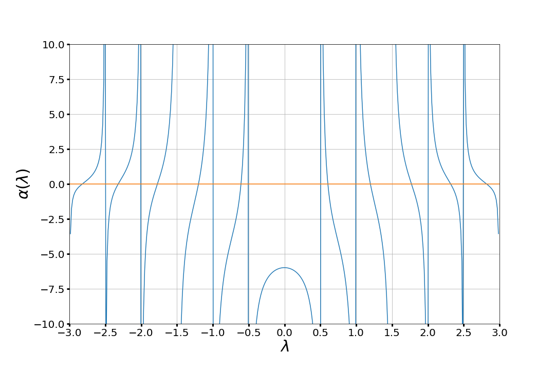
Figure 1: Secular function for $\omega_{c}=0.5$ and $n=1$

The plot in Figure 1 illustrates the properties of $\alpha$ (deduced from Lemma 5.5 and relation (8.4)), most notably that there is unique root (hence an eigenvalue for $\mathbf{H}$) in $(m\omega_{\rm c},(m+1)\omega_{\rm c})$ for $m\geq 1,$ and $((m-1)\omega_{\rm c},m\omega_{\rm c})$ for $m\leq-1$. With a standard numerical method (dichotomy or Newton), we can determine the roots of $\alpha$. For example, with $(n,m)=(1,2)$, we find $\lambda_{1,2}\approx 1.19928.$ This eigenvalue $\lambda_{1,2}$ will be used in all the following numerical tests.

8.2 Solving the linear magnetized Vlasov-Ampère system with a Semi-Lagrangian scheme with splitting

To approximate the linear system (2.17) or (5.1-5.2), we use a semi-Lagrangian scheme [9, 29], which is a classical method to approximate transport equations of the form $\partial_{t}f+E(x,t)\partial_{x}f=0$, coupled with a splitting procedure. A splitting procedure corresponds to approximating the solution of $\partial_{t}f+\mathcal{(A+B)}f=0$ by solving $\partial_{t}f+\mathcal{A}f=0$ and $\partial_{t}f+\mathcal{B}f=0$ one after the other.

Hence, the magnetized Vlasov-Ampère system is split so as to only solve transport equations with constant advection terms.

$$\partial_{t}\left(\begin{array}[]{c}u\\ F\end{array}\right)+\mathcal{(A+B+C+D)}\left(\begin{array}[]{c}u\\ F\end{array}\right)=0,$$

with

$$\mathcal{A}=\left(\begin{array}[]{c}v_{1}\partial_{x}\\ 0\end{array}\right), \ \ \mathcal{B}=\left(\begin{array}[]{c}Fv_{1}e^{-\frac{v_{1}^{2}+v_{2}^{2}}{4}}\\ 1^{*}\int ue^{-\frac{v_{1}^{2}+v_{2}^{2}}{4}}v_{1}dv_{1}dv_{2}\end{array}\right), \mathcal{C}=\left(\begin{array}[]{c}-\omega_{c}v_{2}\partial_{v_{1}}\\ 0\end{array}\right), \ \ \mathcal{D}=\left(\begin{array}[]{c}\omega_{c}v_{1}\partial_{v_{2}}\\ 0\end{array}\right).$$

The algorithm used to solve the linearized magnetized Vlasov-Ampère system can thus be summarized as follows

1. Initialization $\mathbf{U}_{ini}=\left(\begin{array}[]{c}w_{n,m}\\ F_{n}\end{array}\right)$ given in (8.1).

2. Going from $t_{n}$ to $t_{n+1}$

   Assume we know $\mathbf{U}_{n}$, the approximation of $\mathbf{U}=\begin{pmatrix}u\\ F\end{pmatrix}$ at time $t_{n}$.

   • We compute $\mathbf{U}^{*}$ by solving $\partial_{t}\mathbf{U}+\mathcal{A}\mathbf{U}=0$ with a semi-Lagrangian scheme during one time step $\Delta t$ with initial condition $\mathbf{U}^{n}$.

   • We compute $\hat{\mathbf{U}}$ by solving $\partial_{t}\mathbf{U}+\mathcal{B}\mathbf{U}=0$ with a Runge-Kutta 2 scheme during one time step $\Delta t$ with initial condition $\mathbf{U}^{*}$.

   • We compute $\mathbf{U}^{**}$ by solving $\partial_{t}\mathbf{U}+\mathcal{C}\mathbf{U}=0$ with a semi-Lagrangian scheme during one time step $\Delta t$ with initial condition $\hat{\mathbf{U}}$.

   • We compute $\mathbf{U}^{n+1}$ by solving $\partial_{t}\,\mathbf{U}+\mathcal{D}\mathbf{U}=0$ with a semi-Lagrangian scheme during one time step $\Delta t$ with initial condition $\mathbf{U}^{**}$.

8.3 Results for the magnetized Vlasov-Ampère system

The solution of the magnetized Vlasov-Ampère system initialized with an eigenfunctions $\mathbf{U}_{\rm ini}=\left(\begin{array}[]{c}w_{n,m}\\ F_{n}\end{array}\right)$ as in (8.1) is simply given by

$$\mathbf{U}(t)=e^{i\lambda_{n,m}t}\,\mathbf{U}_{\rm ini}.$$ (8.5)

Recall that (8.1) is an eigenfunction of $\mathbf{H}$ with eigenvalue $\lambda_{n,-m}=-\lambda_{n,m}.$ In the following results, we have taken $(n,m)=(1,2)$, $\omega_{c}=0.5$, $N_{x}=33$ (number of points of discretization in position), $N_{v_{1}}=N_{v_{2}}=63$ (number of points of discretization in both velocity variables), $L_{v_{1}}=L_{v_{2}}=10$ (numerical truncation in both velocity variables) and, most importantly, $T_{\rm f}=\frac{\pi}{\lambda_{1,2}}$. This means that $\mathbf{U}(T_{\rm f})=\exp\left(i\frac{\pi}{2}\right)\mathbf{U}_{\rm ini}=i\mathbf{U}_{\rm ini}$, and then, the solution of the system at $t=T_{\rm f}$ corresponds to the initial condition where the real and imaginary parts have been exchanged (up to a sign).

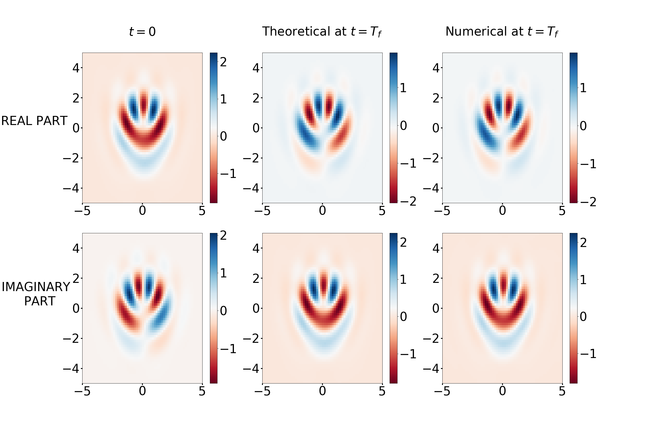
Figure 2: Real and imaginary parts of the first component of $\mathbf{U}(t)$ given by (8.5) in $v_{1}-v_{2}$ plane for $x=0$.

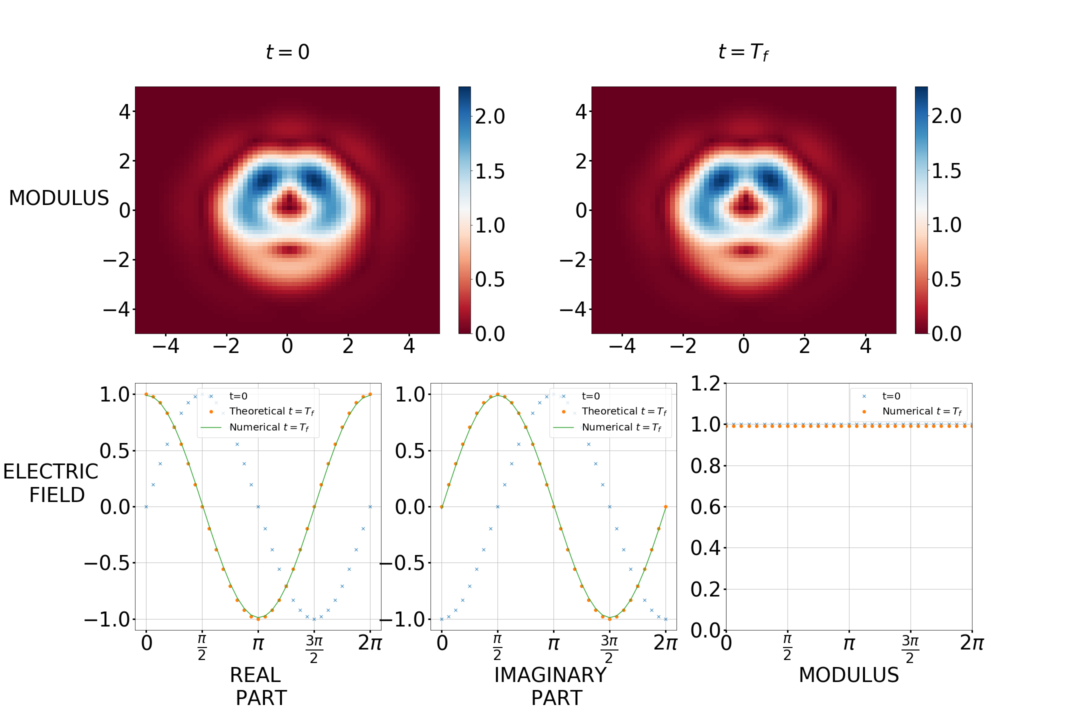
Figure 3: Modulus of the first component of $\mathbf{U}(t)$ given by (8.5) in $v_{1}-v_{2}$ plane for $x=0$, and real and imaginary parts of $F$.

The figures show that the solution of the system behaves according to the theory.

8.4 Results for the non-linear magnetized Vlasov-Poisson system

We now look at how the solution of the non-linear magnetized Vlasov-Poisson system (2.4) behaves when initialized with an eigenfunction of the Hamiltonian $\mathbf{H}$ of the magnetized Vlasov-Ampère system. The idea is that for a certain time, the solution for the non-linear magnetized Vlasov-Poisson system follows the same dynamics as the solution for the linearized magnetized Vlasov-Poisson system. We consider the magnetized Vlasov-Poisson system because it is more convenient for numerical purposes. Recall that the linearized magnetized Vlasov-Poisson and the magnetized Vlasov-Ampère systems are equivalent. Furthermore, the articles [6, 13, 32, 33] have studied the Bernstein-Landau paradox using the magnetized Vlasov-Poisson system. We use almost the same numerical scheme as in the previous subsection to approximate the solution of the system.

The Vlasov equation, namely the first equation in (2.4), in the non-linear magnetized Vlasov-Poisson system is split so as to only solve transport equations with constant advection terms,

$$\partial_{t}u+\mathcal{(A+B+C)}u=0,$$

with $\mathcal{A}=v_{1}\partial_{x}$, $\mathcal{B}=-\left(E+\omega_{c}v_{2}\right)\partial_{v_{1}}$ and $\mathcal{C}=\omega_{c}v_{1}\partial_{v_{2}}$. To update the electric field, the strategy adopted is the same as in [9] where the Poisson equation is solved at each time step. On this numerical computation we consider real valued solutions $f,E.$

Let us denote by $u$ the perturbation of the charge density function, $f,$ and by $F$ be the perturbation of the electric field, $E.$ The functions $u,F$ solve the linearized magnetized Vlasov-Poisson system (2.11). Recall that we proven in Section 5 that the linearized magnetized Vlason-Poisson and magnetized Vlasov-Ampère systems are equivalent. Then, we can use the real part of 8.5 to write the expression of $u,F$ when initializing with, $u_{\rm ini},F_{\rm ini},$ with $u_{\rm ini}=\operatorname{Re}(w_{n,m}),$ $F_{\rm ini}=\operatorname{Re}(F_{n}).$ Recall that $w_{n,m}$, and $F_{n}$ are defined in (8.2). Then, we have,

$$\begin{pmatrix}u(t)\\ F(t)\end{pmatrix}=\operatorname{Re}(\mathbf{U}(t))=\begin{pmatrix}\cos(\lambda_{m}t)\operatorname{Re}(w_{n,m})-\sin(\lambda_{m}t)\operatorname{Im}(w_{n,m})\\ \cos(\lambda_{m}t)\operatorname{Re}(F_{n})-\sin(\lambda_{m}t)\operatorname{Im}(F_{n})\end{pmatrix}$$ (8.6)

where $\mathbf{U}(t)$ is given by (8.5). The objective of this subsection is to show that we can approximate the solution of the non-linear system using (8.6), which means that the solutions of both linear and non-linear systems are close to each other for a certain time.

The algorithm used to solve the non-linear magnetized Vlasov-Poisson system can be summarized as follows:

1. Initialization $f_{ini}=f_{0}+\varepsilon\sqrt{f_{0}}\operatorname{Re}(w_{n,m})$ and $E_{\rm ini}=\varepsilon\operatorname{Re}(F_{n})$ are given, where $\varepsilon$ is a scalar which controls the amplitude of the perturbation. We take $\varepsilon=0.1$.

2. Going from $t_{n}$ to $t_{n+1}$

   Assume we know $f_{n}$ and $E_{n}$, the approximations of $f$ and $E$ at time $t_{n}$.

   • We compute $f^{*}$ by solving $\partial_{t}f+v_{1}\partial_{x}f=0$ with a semi-Lagrangian scheme during one time step $\Delta t$ with initial condition $f_{n}$.

   • We compute $E_{n+1}$ by solving the Poisson equation with $f^{*}$.

   • We compute $\hat{f}$ by solving $\partial_{t}f-(E_{n+1}+\omega_{c}v_{2})\partial_{v_{1}}f=0$ with a semi-Lagrangian scheme during one time step $\Delta t$ with initial condition $f^{*}$.

   • We compute $f^{n+1}$ by solving $\partial_{t}f+\omega_{c}v_{1}\partial_{v_{2}}f=0$ with a semi-Lagrangian scheme during one time step $\Delta t$ with initial condition $\hat{f}$.

As in Subsection  8.3 we take $(n,m)=(1,2)$, $\omega_{c}=0.5$, $N_{x}=33$ (number of points of discretization in position), $N_{v_{1}}=N_{v_{2}}=63$ (number of points of discretization in both velocity variables), $L_{v_{1}}=L_{v_{2}}=10$ (numerical truncation in both velocity variables) and, $T_{\rm f}=\frac{\pi}{\lambda_{1,2}}$. In the following figures, we are comparing respectively the theoretical perturbations, $u,F,$ that are given by (8.6), and the numerical perturbations,

$$u^{n}=\frac{f^{n}-f_{0}}{\varepsilon\sqrt{f_{0}}},\text{\rm and}\,F^{n}=\frac{E^{n}}{\varepsilon},$$

where $f^{n}$ and $E^{n}$ are given by the above algorithm.

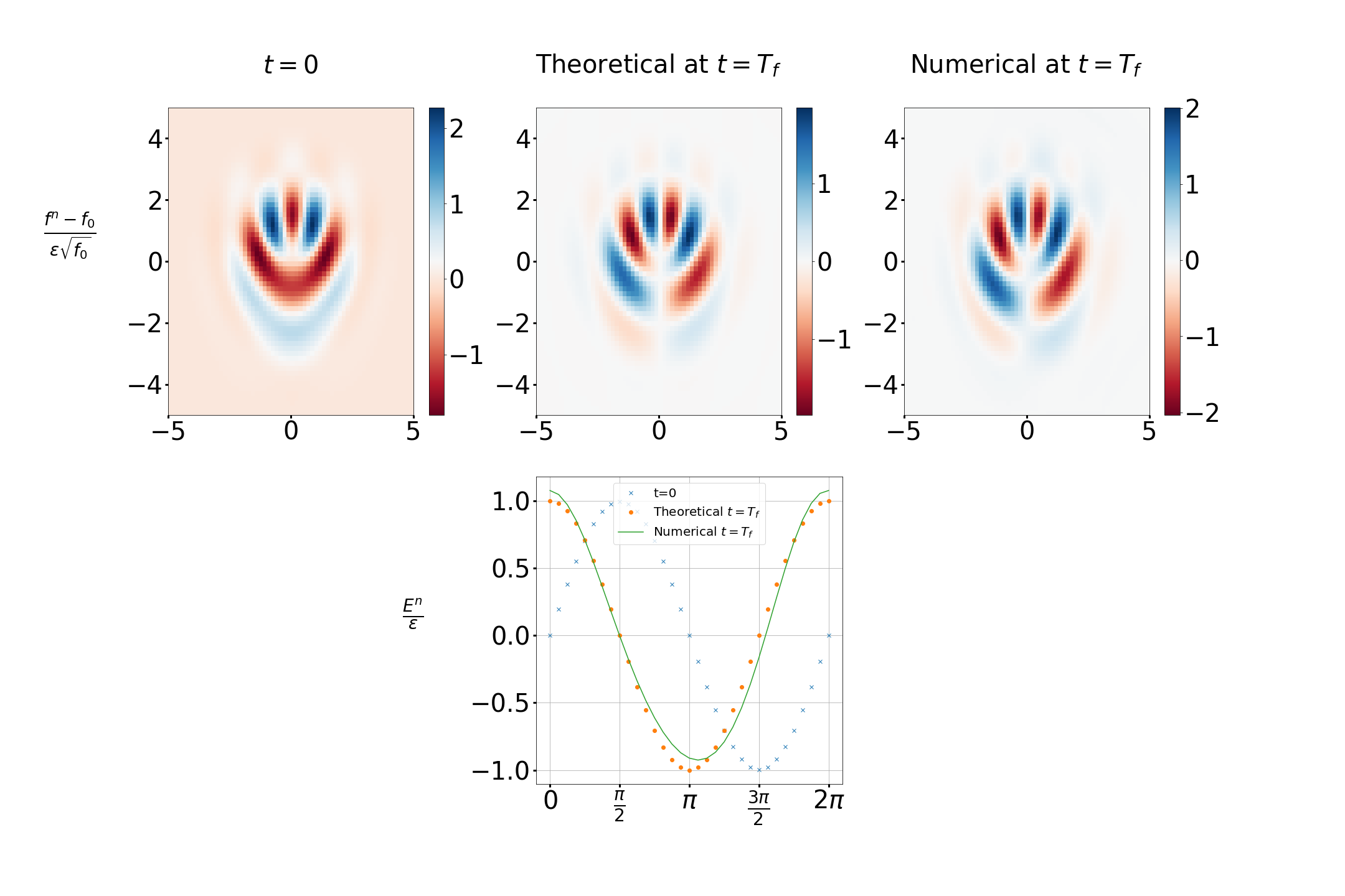
Figure 4: $u$ in $v_{1}-v_{2}$ plane for $x=0$ and electric field $F$.

The figures show that we can approximate the solution of the non-linear magnetized Vlasov-Poisson system using solutions of the linear magnetized Vlasov-Poisson system, initialized with the eigenfunctions of the Hamiltonian, $\mathbf{H}$ of the magnetized Vlasov-Ampère system.

8.5 The Bernstein-Landau paradox

In this subsection we numerically illustrate the Bernstein-Landau paradox, and we compare it with the Landau damping, using the above algorithm (similarly to [13]). In order to compare the numerical solutions to the non-linear Vlasov-Poisson system with the approximate analytical solution found in [28] in the case $\omega_{\rm c}=0,$ we take below the charge of the ions equal to one. With this convention the non-linear Vlasov-Poisson system is written as,

$$\left\{\begin{aligned} &\partial_{t}f+v_{1}\partial_{x}f-E\partial_{v_{1}}f+\omega_{c}\left(-v_{2}\partial_{v_{1}}+v_{1}\partial_{v_{2}}\right)f=0.\\ &\partial_{x}E(t,x)=1-\int_{\mathbb{R}^{2}}\,fdv.\end{aligned}\right.$$ (8.7)

Furthermore, also with the purpose of comparing with the approximate analytical solution of [28], we initialize with the density function $f_{LD}$ given by,

$$f_{LD}(x,v_{1},v_{2})=\frac{1}{2\pi}\left(1+\varepsilon\cos{kx}\right)\,\displaystyle e^{\frac{-v^{2}}{2}},\quad\varepsilon=0.001,k=0.4.$$ (8.8)

In this simulation the position interval is $[0,\frac{2\pi}{k}]$, since we keep periodic solutions. To introduce the approximate analytical solution of [28] let us consider the Vlasov-Poisson system (8.7) with $\omega_{\rm c}=0,$

$$\left\{\begin{aligned} &\partial_{t}f+v_{1}\partial_{x}f-E\partial_{v_{1}}f=0,\\ &\partial_{x}E(t,x)=1-\int_{\mathbb{R}^{2}}\,fdv,\end{aligned}\right.$$ (8.9)

and initialized with (8.8).

Let us look for a solution of the form,

$$f(t,x,v)=f_{1}(t,x,v_{1})\,\frac{1}{\sqrt{2\pi}}\,e^{\frac{-v_{2}^{2}}{2}}.$$ (8.10)

Then, $f(t,x,v)$ satisfies the (8.9) and it is initialized with (8.8) if and only if $f_{1}(t,x,v_{1})$ is a solution of the following Vlasov-Poisson system in one dimension in space and velocity,

$$\left\{\begin{aligned} &\partial_{t}f_{1}+v_{1}\partial_{x}f_{1}-E_{1}\partial_{v_{1}}f_{1}=0,\\ &\partial_{x}E_{1}(t,x)=1-\int_{\mathbb{R}}\,f_{1}dv_{1},\end{aligned}\right.$$ (8.11)

initialized with,

$$f_{1}(0,x,v_{1})=\frac{1}{\sqrt{2\pi}}\left(1+\varepsilon\cos{kx}\right)\displaystyle e^{\frac{-v_{1}^{2}}{2}},\quad\varepsilon=0.001,k=0.4.$$ (8.12)

Furthermore, note that

$$E(t,x)=E_{1}(t,x).$$ (8.13)

Then, we can compute an approximate $E(t,x)$ using the approximate solution to (8.11), (8.12) given in page 58 of [28]. Namely,

$$E(x,t)\approx 4\varepsilon\times 0,424666\exp(-0,0661t)\sin(0,4x)\cos(1,2850t-0,3357725).$$ (8.14)

We have taken the values given in the second line of the table in page 58 of [28]. This approximate solution is a good approximation to the exact solution for large times. Further, (8.14) is a classical test function to highlight Landau damping, more precisely the damping of the electric energy. In the figures below we report (8.14) in the black curves. Moreover, the figure below illustrates how when $\omega_{c}\neq 0$, the damping is replaced by a recurrence phenomenon of period $T_{c}=\frac{2\pi}{\omega_{c}}$, which follows the behaviour observed in [4, 32]. We take $\omega_{\rm c}=0.1,$ and as in Subsection  8.3, we use, $N_{x}=33$ (number of points of discretization in position), $N_{v_{1}}=N_{v_{2}}=63$ (number of points of discretization in both velocity variables), $L_{v_{1}}=L_{v_{2}}=10$ (numerical truncation in both velocity variables).

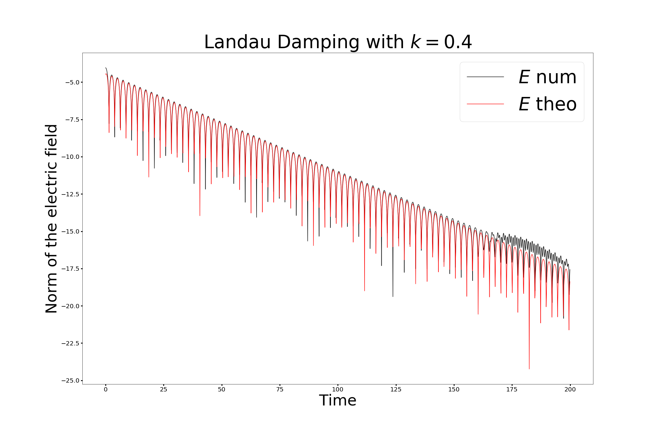
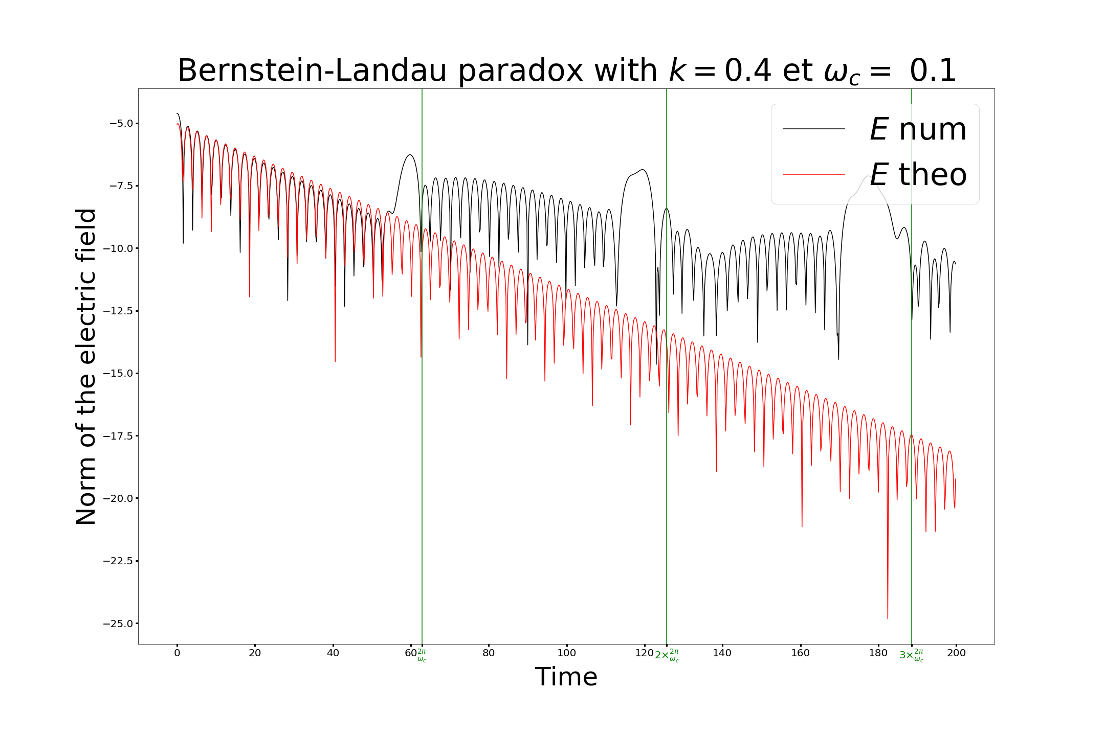
Figure 5: Damped and undamped electric field

The recurrence visible on the right-hand side figure, i.e. the Bernstein paradox, is a fully ”physical” phenomenon originating from the non-zero magnetic field and is to be distinguished from the recurrence in semi-Lagrangian schemes studied in [20], which deals with a purely numerical phenomenon. Let us show that this recurrence is a consequence of our series based on the eigenvectors expansion in the regime of non zero magnetic field. For this purpose, we take the charge of the ions equal to $2\pi,$ and solutions with period $2\pi,$ to be able to use our results of the previous sections. We consider the initial data.

$$\mathbf{G}_{0}:=\left(u_{0}(x,v),F_{0}(x)\right)=\left(e^{\frac{-v^{2}}{4}}\,\cos{lx},-\frac{2\pi}{l}\sin{lx}\right),l\in\mathcal{Z}^{\ast},$$ (8.15)

which satisfies the Gauss law. To compute the electric field with the expansion of the solution to the magnetic Vlasov-Ampère system given in (6.2), (6.4), (6.7) we only need to consider the eigenfunctions with non zero electric field, namely, $\mathbf{F}^{(0}_{n}$ and $\mathbf{Z}_{n,m}.$ Recalling that the electric field is the second component of (6.2) we obtain,

$$F(x,t) =\sum_{n\in\mathbb{Z}^{\ast}}\,\left(\mathbf{G}_{0},\mathbf{F}^{(0}_{n}\right)\,\mathbf{F}_{n}^{(0,2)}(x)+\sum_{n,m\in\mathbb{Z}^{\ast}}\,e^{-i\lambda_{n,m}t}\left(\mathbf{G}_{0},\mathbf{Z}_{n,m}\right)_{\mathcal{H}}\,\mathbf{Z}^{(2)}_{n,m}(x)=$$

$$\left(\mathbf{G}_{0},\mathbf{F}^{(0}_{l}\right)\,\mathbf{F}_{l}^{(0,2)}(x)+\sum_{m\in\mathbb{Z}^{\ast}}\,e^{-i\lambda_{l,m}t}\left(\mathbf{G}_{0},\mathbf{Z}_{l,m}\right)_{\mathcal{H}}\,\mathbf{Z}^{(2)}_{l,m}(x),$$ (8.16)

where we denote by $\mathbf{F}^{(0,2)}_{n},$ respectively, $\mathbf{Z}^{(2)}_{n,m}$ the second component of $\mathbf{F}^{(0)}_{n},$ and of $\mathbf{Z}_{n,m}.$ Then, using (2.10) with $E_{0}=0,$ and (8.5) we get the approximate formula for the electric field,

$$E(x,t)\approx\varepsilon\Re F(t)=\varepsilon\Re\left(\mathbf{G}_{0},\mathbf{F}^{(0}_{l}\right)\,\mathbf{F}_{l}^{(0,2)}(x)+\varepsilon\,\Re\sum_{m\in\mathbb{Z}^{\ast}}\,e^{-i\lambda_{l,m}t}\left(\mathbf{G}_{0},\mathbf{Z}_{l,m}\right)_{\mathcal{H}}\,\mathbf{Z}^{(2)}_{l,m}(x).$$ (8.17)

This approximate formula for the electric field shows the recurrence observed in the right-hand side of figure 5. For clarity, we indicate real part in (8.17), but note that since the initial data $\mathbf{G}_{0}$ in (8.15) is real valued , and the solution to the magnetic Vlasov-Ampére system(2.17) is unique, actually the electric field given by (8.5) is real valued.

Appendix A Technical formulas

In this Appendix we further study the properties of the secular equation (5.49, 5.45, 5.50). For later use we prepare the following result.

PROPOSITION A.1.

Let $a_{n,m},n\in\mathbb{Z}^{\ast},m=1,\dots,$ be the quantity defined in (5.45). Then, there is a constant, $C$, that depends on $n,$ such that,

$$a_{n,m}\leq C\,\frac{1}{\sqrt{m}}\,\left[\frac{en^{2}}{2\omega_{\text{\rm c}}^{2}m}\right]^{m},\qquad m=1,\dots,$$ (A.1)

where $e$ is Euler’s number. In particular, for any $p>0$ there is a constant $C,$ that depends on $n$ and $p,$ such that,

$$a_{n,m}\leq C\frac{1}{m^{p}}.$$ (A.2)

Proof.

By equation (10.22.67) in page 245 of [22]

$$a_{n,m}=e^{\frac{-n^{2}}{\omega_{\text{\rm c}}^{2}}}\,I_{m}\left(\frac{n^{2}}{\omega_{\text{\rm c}}^{2}}\right),$$ (A.3)

with $I_{n}(z)$ a modified Bessel function. Furthermore, by equation (10.41.1) in page 256 of [22],

$$I_{m}\left(\frac{n^{2}}{\omega_{\text{\rm c}}^{2}}\right)=\frac{1}{\sqrt{2\pi m}}\,\left(\frac{en^{2}}{2\omega_{\text{\rm c}}^{2}m}\right)^{m}(1+o(1)),\qquad m\to\infty.$$ (A.4)

Equation (A.1) follows from (A.3) and (A.4). Finally, (A.2) follows from (A.1). ∎

We continue the analysis of the secular equation Let $\lambda_{n,m},m\geq 2$ be the root given in Lemma  5.6. Recall that $\lambda_{n,m}\in(m\omega_{\rm{c}},(m+1)\omega_{\rm{c}}).$ Then, to isolate terms that can be large as $\lambda_{n,m}$ is close to $m\omega_{\rm{c}}$ or to ($m+1)\omega_{\rm{c}},$ we decompose $g(\lambda_{n,m})$ as follows,

$$g(\lambda_{n,m})=g^{(1)}(\lambda_{n,m})+g^{(2)}(\lambda_{n,m})+g^{(3)}(\lambda_{n,m})+g^{(4)}(\lambda_{n,m}),$$ (A.5)

where,

$$g^{(1)}(\lambda_{n,m}):=4\pi\,\sum_{1\leq q\leq m-1}\,\frac{q^{2}\,\omega^{2}_{\text{\rm c}}}{q^{2}\omega^{2}_{\text{\rm c}}-\lambda_{n,m}^{2}}a_{n,q},$$ (A.6)

$$g^{(2)}(\lambda_{n,m}):=4\pi\,\frac{m^{2}\,\omega^{2}_{\text{\rm c}}}{m^{2}\omega^{2}_{\text{\rm c}}-\lambda_{n,m}^{2}}a_{n,m},$$ (A.7)

$$g^{(3)}(\lambda_{n,m}):=4\pi\,\frac{(m+1)^{2}\,\omega^{2}_{\text{\rm c}}}{(m+1)^{2}\omega^{2}_{\text{\rm c}}-\lambda_{n,m}^{2}}a_{n,m+1},$$ (A.8)

$$g^{(4)}(\lambda_{n,m}):=4\pi\,\sum_{q\geq m+2}\,\frac{q^{2}\,\omega^{2}_{\text{\rm c}}}{q^{2}\omega^{2}_{\text{\rm c}}-\lambda_{n,m}}a_{n,q}.$$ (A.9)

LEMMA A.2.

Let $g^{(1)}(\lambda_{n,m})$ be the quantity defined in (A.6). Then, there is a constant $C_{n}$ such that,

$$\left|g^{(1)}(\lambda_{n,m})\right|\leq C_{n}\,\frac{1}{m^{2}},\qquad m\geq 2.$$ (A.10)

Proof.

First suppose that $m$ is even. Then, $m/2$ is an integer, and we can decompose $g^{(1)}(\lambda_{n,m})$ as follows,

$$g^{(1)}(\lambda_{n,m})=g^{(1,1)}(\lambda_{n,m})+g^{(1,2)}(\lambda_{n,m}),$$ (A.11)

where,

$$g^{(1,1)}(\lambda_{n,m}):=4\pi\,\sum_{1\leq q\leq m/2}\,\frac{q^{2}\,\omega^{2}_{\text{\rm c}}}{q^{2}\omega^{2}_{\text{\rm c}}-\lambda_{n,m}^{2}}a_{n,q},$$ (A.12)

and

$$g^{(1,2)}(\lambda_{n,m}):=4\pi\,\sum_{m/2<q\leq m-1}\,\frac{q^{2}\,\omega^{2}_{\text{\rm c}}}{q^{2}\omega^{2}_{\text{\rm c}}-\lambda_{n,m}^{2}}a_{n,q}.$$ (A.13)

Note that,

$$\left|\frac{1}{q^{2}\omega^{2}_{\text{\rm c}}-\lambda_{n,m}^{2}}\right|\leq\frac{2}{m^{2}\omega^{2}_{\text{\rm c}}},\qquad q=1,\dots,\frac{m}{2}.$$ (A.14)

Then, by (A.2), (A.12) and, (A.14)

$$\left|g^{(1,1)}(\lambda_{n,m})\right|\leq 4\pi\,\frac{2}{m^{2}\omega^{2}_{\text{\rm c}}}\sum_{1}^{m/2}\,q^{2}\,\omega^{2}_{\text{\rm c}}\,a_{n,q}\leq C\frac{1}{m^{2}}.$$ (A.15)

Furthermore, we have

$$\left|\frac{1}{q^{2}\omega^{2}_{\text{\rm c}}-\lambda_{n,m}^{2}}\right|\leq\frac{1}{\omega_{\text{\rm c}}}\,\frac{1}{m{\omega_{\text{\rm c}}}},\qquad q=\frac{m}{2},\dots,m-1.$$ (A.16)

Then, by (A.2), (A.13) and, (A.16),

$$\left|g^{(1,2)}(\lambda_{n,m})\right|\leq 4\pi\,\frac{1}{\omega_{\text{\rm c}}}\,\frac{1}{m\omega_{\text{\rm c}}}\,\sum_{m/2<q\leq m-1}\,q^{2}\,\omega^{2}_{\text{\rm c}}a_{n,q}\leq C_{p}\frac{1}{m^{p}},\,p=1,\dots.$$ (A.17)

Equation (A.10) follows from (A.11), (A.15) and, (A.17). In the case where $m$ is odd, $(m-1)/2$ is an integer, and we decompose $g^{(1)}(\lambda_{n,m})$ as in (A.11) with,

$$g^{(1,1)}(\lambda_{n,m}):=4\pi\,\sum_{1\leq q\leq(m-1)/2}\,\frac{q^{2}\,\omega^{2}_{\text{\rm c}}}{q^{2}\omega^{2}_{\text{\rm c}}-\lambda_{n,m}}a_{n,q},$$ (A.18)

and

$$g^{(1,2)}(\lambda_{n,m}):=4\pi\,\sum_{(m-1)/2<q\leq m-1}\,\frac{q^{2}\,\omega^{2}_{\text{\rm c}}}{q^{2}\omega^{2}_{\text{\rm c}}-\lambda_{n,m}^{2}}a_{n,q},$$ (A.19)

and we proceed as in the case of $m$ even. ∎

In the following lemma we estimate $g^{(4)}(\lambda_{n,m}).$

LEMMA A.3.

Let $g^{(4)}(\lambda_{n,m})$ be the quantity defined in (A.9). Then, for every $p>0$ there is a constant $C_{p}$ such that,

$$\left|g^{(4)}(\lambda_{n,m})\right|\leq C_{p}\,\frac{1}{m^{p}},\qquad m\geq 2.$$ (A.20)

Proof.

Note that,

$$\left|\frac{1}{q^{2}\omega^{2}_{\text{\rm c}}-\lambda_{n,m}^{2}}\right|\leq\frac{1}{\omega_{\text{\rm c}}}\,\frac{1}{(m+3){\omega_{\text{\rm c}}}},\qquad q\geq m+2.$$ (A.21)

Equation (A.20) follows from (A.2), (A.9) and, (A.21). ∎

In the following lemma we estimate how $\lambda_{n,m}$ approaches $m\omega_{\text{\rm c}}$ as $m\to\pm\infty.$

LEMMA A.4.

We have,

$$\lambda_{n,m}=m\omega_{\text{\rm c}}+2\pi m\,\omega_{\text{\rm c}}\,\frac{a_{n,|m|}}{n^{2}}+a_{n,|m|}\,O\left(\frac{1}{|m|}\right),\qquad m\to\pm\infty.$$ (A.22)

Proof.

Note that since $\lambda_{n,-m}=-\lambda_{n,m}$ it is enough to prove equation (A.22) when $m\to\infty.$

Using (A.10) and (A.20) we write (5.50) as follows

$$4\pi\,\frac{m^{2}\,\omega^{2}_{\text{\rm c}}}{\lambda_{n,m}^{2}-m^{2}\omega^{2}_{\text{\rm c}}}a_{n,m}=n^{2}+g^{(3)}(\lambda_{n,m})+O\left(\frac{1}{m^{2}}\right),\qquad m\to\infty.$$ (A.23)

Moreover, as $g^{(3)}(\lambda_{n,m})\geq 0,$ we get,

$$4\pi\,\frac{m^{2}\,\omega^{2}_{\text{\rm c}}}{\lambda_{n,m}^{2}-m^{2}\omega^{2}_{\text{\rm c}}}a_{n,m}\geq n^{2}+O\left(\frac{1}{m^{2}}\right),\qquad m\to\infty.$$

Then, there is an $m_{0}$ such that $4\pi\,\frac{m^{2}\,\omega^{2}_{\text{\rm c}}}{\lambda_{n,m}^{2}-m^{2}\omega^{2}_{\text{\rm c}}}a_{n,m}\geq\frac{\pi}{4}$, $m\geq m_{0}$, and then, $\lambda_{n,m}^{2}\leq m^{2}\omega^{2}_{\text{\rm c}}+16m^{2}\,\omega^{2}_{\text{\rm c}}\,a_{n,m}$, $m\geq m_{0}$, and taking the square root we obtain

$$m\omega_{\text{\rm c}}\leq\lambda_{n,m}\leq m\omega_{\text{\rm c}}\sqrt{1+16\,a_{n,m}},\qquad m\geq m_{0}.$$ (A.24)

This already shows that $\lambda_{n,m}$ is asymptotic to $\omega_{\text{\rm c}}$ for large $m.$ However, we can improve this estimate to obtain (A.22). By (A.2) and (A.24) for every $p>0,$

$$\left((m+1)\omega_{\text{\rm c}}-\lambda_{n,m}\right)^{-1}=\frac{1}{\omega_{\text{\rm c}}}\left(1+O\left(\frac{1}{m^{p}}\right)\right),\qquad m\to\infty.$$ (A.25)

Further, introducing (A.8) and (A.25) into (A.23), and using (A.2) we obtain,

$$4\pi\,\frac{m^{2}\,\omega^{2}_{\text{\rm c}}}{\lambda_{n,m}^{2}-m^{2}\omega^{2}_{\text{\rm c}}}a_{n,m}=n^{2}+O\left(\frac{1}{m^{2}}\right),\qquad m\to\infty.$$ (A.26)

We rearrange (A.26) as follows,

$$\lambda_{n,m}-m\omega_{\text{\rm c}}=\frac{4\pi}{n^{2}}\,\frac{m^{2}\,\omega^{2}_{\text{\rm c}}}{\lambda_{n,m}+m\omega_{\text{\rm c}}}a_{n,m}+\frac{1}{n^{2}}\,(\lambda_{n,m}-m\omega_{\text{\rm c}})\,O\left(\frac{1}{m^{2}}\right),\qquad m\to\infty.$$ (A.27)

By (A.24)

$$\lambda_{n,m}-m\omega_{\text{\rm c}}\leq m\omega_{\text{\rm c}}\,O\left(a_{n,m}\right),\qquad m\to\infty.$$ (A.28)

Further,

$$\left(\lambda_{n,m}+m\omega_{\text{\rm c}}\right)^{-1}=\left(2m\omega_{\text{\rm c}}+\lambda_{n,m}-m\omega_{\text{\rm c}}\right)^{-1}=\frac{1}{2m\omega_{\text{\rm c}}}\,(1+O\left(a_{n,m}\right)),\qquad m\to\infty.$$ (A.29)

Expansion (A.22) follows from (A.28) and, (A.29). ∎

Appendix B A family of stationary solutions

In this appendix we construct explicitly a family of time-independent solutions to the linearized magnetized Vlasov-Poisson system. We first construct the family in dimension 1+2 (one dimension in space, two dimensions in velocity), that is the situation that we consider in our work. Then, we generalize our family of solutions to the case dimension 3+3 (three dimensions in space, three dimensions in velocity) that is the case considered by Bedrossian and Wang [5].

B.1 Dimension 1+2

For the purpose of making the comparison with [5] more transparent we consider the Vlasov equation,

$$\partial_{t}f+v_{1}\partial_{x}f+\mathbf{F}\cdot\nabla_{v}f=0,$$ (B.1)

with the electromagnetic Lorenz force,

$$\mathbf{F}(t,x)=\frac{q}{m}\left(\mathbf{E}(t,x)+v\times\mathbf{B}_{0}(t,x)\right).$$ (B.2)

Taking $\mathbf{B}_{0}\neq 0$ the plasma is magnetized. The variable $x$ is in the periodic torus $x\in\mathcal{T}=[0,2\pi]_{\rm per}$. The velocity variables are $(v_{1},v_{2})\in\mathbb{R}^{2}$. We take the charge $q>0$ (Remark 2.1) the mass $m>0,$ and we assume, as before, that the magnetic field $\mathbf{B}(t,\mathbf{x})=\mathbf{B}_{0}$ is constant in space-time. We suppose again that the two-dimensional velocity $v$ is perpendicular to the constant magnetic field, i.e., $\mathbf{B}_{0}=(0,0,B_{0}),B_{0}>0.$ Moreover, we assume that the electric field is directed along the first coordinate axis, $\mathbf{E}(t,x)=(E(t,x),0,0),$ that it has mean zero,

$$\int_{\mathcal{T}}\,E(t,x)\,dx=0,$$

and that it satisfies the Gauss law,

$$\partial_{x}E(t,x)=\frac{1}{4\pi}\,\left(-1+q\int_{\mathbb{R}^{2}}\,fdv\right),$$ (B.3)

where as in [5] we introduced the factor $\frac{1}{4\pi}$ in the right-hand side of the Gauss law, and we have taken the charge of the heavy particles equal to minus one. See Remark 2.1.

We linearize the equations around a homogeneous Maxwellian equilibrium state $\tilde{f}_{0}(v),$ where,

$$\tilde{f}_{0}(v):=\frac{1}{2\pi}e^{\frac{-v^{2}}{2}}.$$

We take as equilibrium state $\tilde{f}_{0}(v):=\frac{1}{2\pi}e^{\frac{-v^{2}}{2}}$ to make the comparison with the results of [5] more transparent. This corresponds to the expansion,

$$f(t,x,v)=\tilde{f}_{0}(v)+\varepsilon h(t,x,v)+O(\varepsilon^{2}),$$ (B.4)

and

$$E(t,x)=E_{0}+\varepsilon F(t,x)+O(\varepsilon^{2}),$$ (B.5)

with a null reference electric field $E_{0}=0$. Inserting (B.4) and (B.5) into (B.1)-(B.3), and keeping the terms up to linear in $\varepsilon,$ we obtain the linearized magnetized Vlasov-Poisson system

$$\left\{\begin{aligned} &\partial_{t}h+v_{1}\partial_{x}h-\frac{q}{m}Fv_{1}{\tilde{f}_{0}}-\frac{q}{m}B_{0}\left(-v_{2}\partial_{v_{1}}+v_{1}\partial_{v_{2}}\right)h=0,\\ &\partial_{x}F=\frac{q}{4\pi}\,\int_{\mathbb{R}^{2}}h\,dv_{1}dv_{2},\int_{\mathcal{T}}\,F(t,x)\,dx=0.\end{aligned}\right.$$ (B.6)

As we look for time-independent solutions, we have to solve,

$$\left\{\begin{aligned} &v_{1}\partial_{x}h-\frac{q}{m}Fv_{1}{\tilde{f}_{0}}-\frac{q}{m}B_{0}\left(-v_{2}\partial_{v_{1}}+v_{1}\partial_{v_{2}}\right)h=0,\\ &\partial_{x}F=\frac{q}{4\pi}\int_{\mathbb{R}^{2}}h\,dv_{1}\,dv_{2},\qquad\int_{\mathcal{T}}\,F(t,x)\,dx=0.\end{aligned}\right.$$ (B.7)

Note that,

$$\left(-v_{2}\partial_{v_{1}}+v_{1}\partial_{v_{2}}\right)\tilde{f}_{0}(v_{1},v_{2})=0.$$ (B.8)

Our objective hereafter is to construct a family of non trivial smooth solutions to (B.7) that have fast decay in velocity.

LEMMA B.1.

There exists an explicit family of non trivial smooth solutions $(h,F)$ to the time-independent linearized magnetized Vlasov-Poisson system (B.7), where $F=-\varphi^{\prime}(x),$ with $\varphi\in C^{\infty}(\mathcal{T}),$ and where the function $h$ can be taken with $l$ continuous derivates with respect to $v,l=1,2,\dots,$ or infinitely differentiable with respect to $v.$ Moreover, for each fixed $x\in\mathcal{T},h\in L^{1}(\mathbb{R}^{2}).$ Further, the absolute value of $h$ and of all its derivatives can be taken bounded by Gaussian functions of $v,$ uniformly in $x\in\mathcal{T}.$ Moreover, $h+\frac{q}{m}\varphi f_{0}$ can be taken with compact support in $\mathbf{v}$, uniformly in $x\in\mathcal{T}.$

Proof.

We introduce an electric potential $\varphi\in C^{1}(\mathcal{T})$ as

$$F(x)=-\varphi^{\prime}(x),$$

with $\varphi(2\pi)=\varphi(0)$ and $\varphi^{\prime}(2\pi)=\varphi^{\prime}(0).$ Plugging in the first equation in (B.7), we obtain

$$v_{1}\partial_{x}\left[h(x,v_{1},v_{2})+\frac{q}{m}\varphi(x)\tilde{f}_{0}(v_{1},v_{2})\right]-\frac{q}{m}B_{0}\left(-v_{2}\partial_{v_{1}}+v_{1}\partial_{v_{2}}\right)h=0.$$

Let us define

$$G(x,v_{1},v_{2})=h(x,v_{1},v_{2})+\frac{q}{m}\varphi(x)\tilde{f}_{0}(v_{1},v_{2}).$$ (B.9)

Since we have (B.8), $G$ satisfies the equation

$$v_{1}\partial_{x}G(x,v_{1},v_{2})-\frac{q}{m}B_{0}\left(-v_{2}\partial_{v_{1}}+v_{1}\partial_{v_{2}}\right)G(x,v_{1},v_{2})=0.$$ (B.10)

Let us make another change of function which is valid since $B_{0}\neq 0,$

$$H(x,v_{1},v_{2})=G(x-\frac{m\,v_{2}}{\,qB_{0}},v_{1},v_{2})\Longleftrightarrow G(x,v_{1},v_{2})=H(x+\frac{m\,v_{2}}{q\,B_{0}},v_{1},v_{2}).$$ (B.11)

The equation (B.10) is rewritten as

$$\frac{q}{m}\omega_{c}\left(-v_{2}\partial_{v_{1}}+v_{1}\partial_{v_{2}}\right)H(x,v_{1},v_{2})=0.$$ (B.12)

Under this form, it is easy to find a general solution which writes

$$H(x,v_{1},v_{2})=K(x,v_{1}^{2}+v_{2}^{2})$$

where $K$ is an arbitrary smooth function which decreases sufficiently fast at infinity with respect to its second variable. For example, we can take,

$$K(x,v_{1}^{2}+v_{2}^{2})=e^{inx}g(v_{1}^{2}+v_{2}^{2}),\qquad n\in\mathcal{Z}\setminus\{0\},$$ (B.13)

where $g(v_{1}^{2}+v_{2}^{2})\in C^{l}(\mathbb{R}^{2}),l=1,2,\dots,$ or $g(v_{1}^{2}+v_{2}^{2})\in C^{\infty}(\mathbb{R}^{2}),$ and $g(v_{1}^{2}+v_{2}^{2})\in L^{1}(\mathbb{R}^{2}).$ For example, $g$ can be taken with compact support, or a Gaussian. Going back to the perturbation $h$, one obtains the representation formula

$$h(x,v_{1},v_{2})=-\frac{q}{m}\varphi(x)\tilde{f}_{0}(v_{1},v_{2})+K(x+\frac{m\,v_{2}}{q\,B_{0}},v_{1}^{2}+v_{2}^{2}),$$

where the electric potential $\varphi$ remains to be determined. All functions $h$ of this form satisfy the first equation of (B.7).
It remains to verify the Gauss law, that is the second equation of (B.7). The right-hand side of the Gauss law is

$$\frac{q}{4\pi}\int_{\mathbb{R}^{2}}h\,dv_{1}\,dv_{2}=\frac{q}{4\pi}\left(-\frac{q}{m}\,\varphi(x)+\int_{\mathbb{R}^{2}}\,K(x+\frac{m\,v_{2}}{q\,B_{0}},v_{1}^{2}+v_{2}^{2})\,dv_{1}\,dv_{2}\right).$$

So the Gauss law is rewritten as

$$-\varphi^{\prime\prime}(x)+\frac{q^{2}}{4\pi m}\,\varphi(x)=\frac{q}{4\pi}\,\int_{\mathbb{R}^{2}}K(x+\frac{m\,v_{2}}{q\,B_{0}},v_{1}^{2}+v_{2}^{2})\,dv_{1}\,dv_{2}.$$

Using (B.13), one gets

$$-\varphi^{\prime\prime}(x)+\frac{q^{2}}{4\pi m}\varphi(x)=\frac{q}{4\pi}e^{inx}\int_{\mathbb{R}^{2}}\displaystyle e^{in\frac{mv_{2}}{qB_{0}}}g(v_{1}^{2}+v_{2}^{2})\,dv_{1}\,dv_{2}.$$

This is an equation for the electric potential. The periodic solution is explicit,

$$\varphi(x)=\frac{1}{n^{2}+\frac{q^{2}}{4\pi m}}\,\frac{q}{4\pi}\,e^{inx}\,\int_{\mathbb{R}^{2}}\displaystyle e^{in\frac{mv_{2}}{qB_{0}}}g(v_{1}^{2}+v_{2}^{2})dv_{1}dv_{2}.$$ (B.14)

The remaining properties of the solution $(h,F)$ follow immediately from the explicit representation of $(h,F).$ ∎

Remark that the solutions given by Lemma B.1 satisfy,

$$\int_{\mathcal{T}}h(x,v_{1},v_{2})\,dx=0,$$

and in particular,

$$\int_{\mathcal{T}\times\mathbb{R}^{2}}\,h(x,v_{1},v_{2})\,dx\,dv_{1}\,dv_{2}=0.$$

The solutions given by Lemma B.1 are in agreement with (6.1), (6.2), (6.4), (6.7), and also with (6.14), (6.15), (6.16).

B.2 Dimension 3+3

We now consider solutions to the magnetized Vlasov-Poisson system in $\mathcal{T}^{3}\times\mathbb{R}^{3},$ where $\mathcal{T}^{3}$ is the three-dimensional torus, $\mathcal{T}^{3}:=[0,2\pi]_{\rm per}^{3}.$ We denote $\mathbf{x}:=(x,y,z)\in\mathcal{T}^{3},$ and $\mathbf{v}=(v_{1},v_{2},v_{3})\in\mathbb{R}^{3}.$ The Vlasov equation is given by,

$$\partial_{t}f(t,\mathbf{x},\mathbf{v})+\mathbf{v}\cdot\nabla_{\mathbf{x}}f(t,\mathbf{x},\mathbf{v})+\mathbf{F}(t,\mathbf{x})\cdot\nabla_{\mathbf{v}}f(t,\mathbf{x},\mathbf{v})=0,$$ (B.15)

with the electromagnetic Lorenz force,

$$\mathbf{F}(t,\mathbf{x})=\frac{q}{m}\left(\mathbf{E}(t,\mathbf{x})+\mathbf{v}\times\mathbf{B}_{0}(t,\mathbf{x})\right),$$ (B.16)

where $q>0,m>0,$ and we assume, as before, that the magnetic field $\mathbf{B}(t,\mathbf{x})=\mathbf{B}_{0}$ is constant in space-time, and that it is directed along the third coordinate, i.e., $\mathbf{B}_{0}=(0,0,B_{0}),B_{0}>0.$ Moreover, we assume that the electric field satisfies the Gauss law,

$$\nabla_{\mathbf{x}}\cdot\mathbf{E}(t,\mathbf{x})=\frac{1}{4\pi}\rho(t,\mathbf{x}),\qquad\rho(t,\mathbf{x}):=\,[-1+q\int_{\mathbb{R}^{3}}\,f(t,\mathbf{x},\mathbf{v})\,d^{3}\mathbf{v}].$$ (B.17)

Further, we assume that the electric field has mean zero,

$$\int_{\mathcal{T}^{3}}\,\mathbf{E}(t,\mathbf{x})\,d^{3}\mathbf{x}=0.$$ (B.18)

We linearize equations (B.15)-(B.18) around a homogeneous Maxwellian equilibrium state $f^{0}(\mathbf{v}),$ where,

$$f^{0}(\mathbf{v}):=\tilde{f}_{0}(v_{1},v_{2})\ \frac{1}{\sqrt{2\pi T_{\parallel}}}\,e^{\frac{-v^{2}_{3}}{2T_{\parallel}}},$$

where $T_{\parallel}>0$ is the temperature along the magnetic field. This amounts to take $\tilde{f}=0$ in (1.2). This corresponds to the expansion,

$$f(t,\mathbf{x},\mathbf{v})=f^{0}(\mathbf{v})+\varepsilon\mathcal{G}(t,\mathbf{x},\mathbf{v})+O(\varepsilon^{2}),$$ (B.19)

and

$$\mathbf{E}(t,\mathbf{x})=\mathbf{E}_{0}+\varepsilon\mathcal{F}(t,\mathbf{x})+O(\varepsilon^{2}),$$ (B.20)

with a null reference electric field $\mathbf{E}_{0}=0$. Inserting (B.19) and (B.20) into (B.15)-(B.17), and keeping the terms up to linear in $\varepsilon,$ we obtain the linearized magnetized Vlasov-Poisson system,

$$\left\{\begin{aligned} &\partial_{t}\mathcal{G}(t,\mathbf{x},\mathbf{v})+\mathbf{v}\cdot\nabla_{\mathbf{x}}\mathcal{G}(t,\mathbf{x},\mathbf{v})+\frac{q}{m}\mathcal{F}(t,\mathbf{x})\cdot\nabla_{\mathbf{v}}{f^{0}(\mathbf{v})}+\frac{q}{m}\mathbf{v}\times\mathbf{B}_{0}\cdot\nabla_{\mathbf{v}}\mathcal{G}(t,\mathbf{x},\mathbf{v})=0,\\ &\nabla_{\mathbf{x}}\cdot\mathcal{F}(t,\mathbf{x})=\,\frac{q}{4\pi}\,\rho(t,\mathbf{x}),\qquad\rho(t,\mathbf{x}):=\int_{\mathbb{R}^{3}}\,\mathcal{G}(t,\mathbf{x},\mathbf{v})\,d^{3}\mathbf{v},\qquad\int_{\mathcal{T}^{3}}\,\mathcal{F}(t,\mathbf{x})\,d^{3}\mathbf{x}=0.\end{aligned}\right.$$ (B.21)

We look for solutions to (B.21) that satisfy,

$$\int_{\mathcal{T}^{3}\times\mathbb{R}^{3}}\,\mathcal{G}(t,\mathbf{x},\mathbf{v})\,d^{3}\mathbf{x}\,d^{3}\mathbf{v}=0.$$ (B.22)

Under the condition (B.22) the Gauss law, that is the second equation in (B.21), is equivalent to the following equation,

$$\mathcal{F}(t,\mathbf{x})=-\nabla_{\mathbf{x}}\,\int_{\mathcal{T}^{3}}\,W(\mathbf{x}-\mathbf{y})\,\rho(t,\mathbf{y})\,d^{3}\mathbf{y},$$ (B.23)

where,

$$W(\mathbf{x}):=\frac{q}{4\pi}\,\frac{1}{(2\pi)^{3}}\,\sum_{\mathbf{k}\in\mathbb{Z}^{3}\setminus\{0\}}\,\frac{1}{|\mathbf{k}|^{2}}\,e^{ik\cdot\mathbf{x}}.$$

Since we are looking for time-independent solutions we have to solve,

$$\left\{\begin{aligned} &\mathbf{v}\cdot\nabla_{\mathbf{x}}\mathcal{G}(t,\mathbf{x},\mathbf{v})+\frac{q}{m}\mathcal{F}(t,\mathbf{x})\cdot\nabla_{\mathbf{v}}{f^{0}(\mathbf{v})}+\frac{q}{m}\mathbf{v}\times\mathbf{B}_{0}\cdot\nabla_{\mathbf{v}}\mathcal{G}(t,\mathbf{x},\mathbf{v})=0,\\ &\nabla_{\mathbf{x}}\cdot\mathcal{F}(t,\mathbf{x})=\frac{q}{4\pi}\,\rho(t,\mathbf{x}),\qquad\rho(t,\mathbf{x}):=\int_{\mathbb{R}^{3}}\,\mathcal{G}(t,\mathbf{x},\mathbf{v})\,d^{3}\mathbf{v},\qquad\int_{\mathcal{T}^{3}}\,\mathcal{F}(t,\mathbf{x})\,d^{3}\mathbf{x}=0.\end{aligned}\right.$$ (B.24)

Let $(h,F)$ be one of the solutions to (B.7) given by Lemma B.1. We define,

$$\mathcal{G}(\mathbf{x},\mathbf{v})=h(x,v_{1},v_{2})\,\frac{1}{\sqrt{2\pi T_{\parallel}}}\,e^{\frac{-v^{2}_{3}}{2T_{\parallel}}},\mbox{and }\mathcal{F}(\mathbf{x})=\left(\begin{array}[]{ccc}F(x)\\ 0\\ 0\end{array}\right).$$ (B.25)

LEMMA B.2.

Let $(h(x,v_{1},v_{2}),F(x))$ be one of the solutions to the time-independent linearized magnetized Vlasov-Poisson system (B.7) given by Lemma B.1. Then, the pair $(\mathcal{G}(\mathbf{x},\mathbf{v}),\mathcal{F}(\mathbf{x}))$ defined in (B.25) is a solution to the time-independent linearized magnetized Vlasov-Poisson system (B.24) in $\mathcal{T}^{3}\times\mathbb{R}^{3},$ with $\mathcal{F}\in C^{\infty}(\mathcal{T}^{3}),$ and where the function $h$ can taken with $l$ continuous derivates with respect to $\mathbf{v},l=1,2,\dots,$ or infinitely differentiable with respect to $\mathbf{v}.$ Moreover, for each fixed $x\in\mathcal{T}^{3},h\in L^{1}(\mathbb{R}^{3}).$ Further, the absolute value of $h$ and of all its derivatives can be taken bounded by Gaussian functions of $\mathbf{v},$ uniformly in $\mathbf{x}\in\mathcal{T}^{3}.$ Further, the solution $(\mathcal{G}(\mathbf{x},\mathbf{v}),\mathcal{F}(\mathbf{x}))$ satisfies (B.22).

Proof.

We detail the calculations for the convenience of the reader. One has

$$\begin{array}[]{lll}\mathbf{v}\cdot\nabla_{\mathbf{x}}\mathcal{G}(x,y,z,v_{1},v_{2},v_{3})=v_{1}\partial_{x}h(x,v_{1},v_{2})\ \frac{1}{\sqrt{2\pi T_{\parallel}}}\,e^{\frac{-v^{2}_{3}}{2T_{\parallel}}},\\ \\ \nabla_{\mathbf{v}}\mathcal{G}(x,y,z,v_{1},v_{2},v_{3})=\left(\begin{array}[]{ccc}\partial_{v_{1}}h(x,v_{1},v_{2})\ \frac{1}{\sqrt{2\pi T_{\parallel}}}\,e^{\frac{-v^{2}_{3}}{2T_{\parallel}}}\\ \\ \partial_{v_{2}}h(x,v_{1},v_{2})\ \frac{1}{\sqrt{2\pi T_{\parallel}}}\,e^{\frac{-v^{2}_{3}}{2T_{\parallel}}}\\ \\ h(x,v_{1},v_{2})\ \partial_{v_{3}}\frac{1}{\sqrt{2\pi T_{\parallel}}}\,e^{\frac{-v^{2}_{3}}{2T_{\parallel}}}\\ \end{array}\right),\\ \\ \mathcal{F}(x,y,z)\cdot\nabla_{\mathbf{v}}f^{0}=-F(x)\,v_{1}\,f^{0},\\ \mathbf{v}\times\mathbf{B}_{0}=\left(\begin{array}[]{ccc}B_{0}v_{2}\\ \\ -B_{0}v_{1}\\ \\ 0\end{array}\right),\\ \\ (\mathbf{v}\times\mathbf{B}_{0})\cdot\nabla_{\mathbf{v}}\mathcal{G}(x,y,z,v_{1},v_{2},v_{3})=B_{0}\left(v_{2}\partial_{v_{1}}-v_{1}\partial_{v_{2}}\right)h(x,v_{1},v_{2})\frac{1}{\sqrt{2\pi T_{\parallel}}}\,e^{\frac{-v^{2}_{3}}{2T_{\parallel}}}.\end{array}$$ (B.26)

Therefore, by (B.26) one gets the first equation in the linearized magnetized Vlasov-Poisson system (B.24),

$$\mathbf{v}\cdot\nabla_{\mathbf{x}}\mathcal{G}(t,\mathbf{x},\mathbf{v})+\frac{q}{m}\mathcal{F}(t,\mathbf{x})\cdot\nabla_{\mathbf{v}}{f^{0}(v)}+\frac{q}{m}\mathbf{v}\times\mathbf{B}_{0}\cdot\nabla_{\mathbf{v}}\mathcal{G}(t,\mathbf{x},\mathbf{v})=0.$$ (B.27)

Moreover, one has $\nabla_{\mathbf{x}}\cdot\mathcal{F}(\mathbf{x})=\partial_{x}F(x),$ and

$$\begin{array}[]{lll}\int_{\mathbb{R}^{3}}\mathcal{G}(\mathbf{x},\mathbf{v})\,d^{3}\mathbf{v}&=&\int_{\mathbb{R}^{2}}h(x,v_{1},v_{2})dv_{1}dv_{2}\times\int_{\mathbb{R}}\,\frac{1}{\sqrt{2\pi T_{\parallel}}}\,e^{\frac{-v^{2}_{3}}{2T_{\parallel}}}\,dv_{3}\\ &=&\int_{\mathbb{R}^{2}}h(x,v_{1},v_{2})dv_{1}dv_{2}.\end{array}$$

So one obtains immediately the Gauss law

$$\nabla_{\mathbf{x}}\cdot\mathcal{F}(\mathbf{x})=\frac{q}{4\pi}\,\rho(t,\mathbf{x}).$$ (B.28)

The fact that (B.22) holds, and the properties of the solution $(\mathcal{G},\mathcal{F})$ stated in the lemma hold, follow immediate from the definition of the pair $(h,F).$ ∎

The solutions $(\mathcal{G},\mathcal{F}),$ given by Lemma B.2, to the time-independent linearized magnetized Vlasov-Poisson system (B.24), and that fulfill (B.22), satisfy the assumption of Theorem 1 of Bedrossian and Wang, [5] (see Theorem 1.1 above). For example, we can take $g(v_{1}^{2}+v_{2}^{2})=e^{-v_{1}^{2}+v_{2}^{2}}.$ Moreover, the charge density fluctuation is independent of $y$ and $z,$ and is given by,

$$\rho(x)=e^{inx}\left[\frac{1}{n^{2}+\frac{q^{2}}{4\pi m}}\,\frac{-q^{2}}{4\pi m}+1\right]\int_{\mathbb{R}^{2}}\,e^{in\frac{m\,v_{2}}{q\,B_{0}}}\,g(v_{1}^{2}+v_{2}^{2})\,dv_{1}dv_{2}.$$ (B.29)

The Fourier coefficient $\hat{\rho}(n,0,0)$ is, in general, not zero, and it is given by,

$$\hat{\rho}(n,0,0)=(2\pi)^{3}\,\left[\frac{1}{n^{2}+\frac{q^{2}}{4\pi m}}\,\frac{-q^{2}}{4\pi m}+1\right]\int_{\mathbb{R}^{2}}\,e^{in\frac{m\,v_{2}}{q\,B_{0}}}\,g(v_{1}^{2}+v_{2}^{2})\,dv_{1}dv_{2}.$$ (B.30)

B.3 Limit $B_{0}\to 0$

An interesting question is passing to the limit $B_{0}\to 0$ in the right-hand side of (B.14). One has weak convergence to zero of the right-hand side under standard integrability conditions on $g$ since

$$\underset{B_{0}\to 0}{\lim}\int_{\mathbb{R}^{2}}e^{in\frac{mv_{2}}{qB_{0}}}g(v_{1}^{2}+v_{2}^{2})dv_{1}dv_{2}=0$$

because of the oscillating term $e^{in\frac{mv_{2}}{qB_{0}}}.$ Therefore, by (B.14) the solutions of (B.7) given by Lemma B.1. satisfy

$$\underset{B_{0}\to 0}{\varphi}=0.$$

The weak limit recovers the classical results in the non magnetized case.

Acknowledgement This paper was partially written while Ricardo Weder was visiting the Institut de Mathématique d’Orsay, Université Paris-Saclay. Ricardo Weder thanks Christian Gérard for his kind hospitality. Frédérique Charles, Bruno Després and Alexandre Rege acknowledge the support of the MUFFIN ANR project under contract number ANR-19-CE46-0004.

References

- [1] M. Abramovitz, and I.A. Stegun, Handbook of Mathematical Functions with Formulas Graphs and Mathematical Tables, National Bureau of Standards, USA, 1972,
- [2] R. A. Adams, and J. J. F. Fournier, Sobolev Spaces, Elsevier Science, Oxford, U.K., 2003.
- [3] A. V. Antonov, Remarks on the problem of stability in stellar dynamics, Soviet. Astr., A-J. 4 (5), 859-867, 1961.
- [4] D.E. Baldwin and G. Rowlands, Plasma Oscillations Perpendicular to a Weak Magnetic Field, The Physics of Fluids 9, 2444, 1966.
- [5] J. Bedrossian and F. Wang, The Linearized Vlasov and Vlasov-Fokker-Planck Equations in a Uniform Magnetic Field, J. Stat. Phys. 178, 552-594, 2020.
- [6] I. B. Bernstein, Waves in a plasma in a magnetic field, Phys. Rev., 109 (1), 10-21, 1958.
- [7] M. S. Birman, and M. Z. Solomjak, Spectral Theory of Self-Adjoint Operators in Hilbert Space, D. Reidel, Dordrecht, 1987.
- [8] F. Chen, Introduction to Plasma Physics and Controlled Fusion, Springer New-York 1984.
- [9] M. Z. Cheng, G. Knorr, The Integration of the Vlasov Equation in Configuration Space, Journal of Computational Physics Vol. 22, 1976.
- [10] P. Degond, Spectral theory of the linearized Vlasov-Poisson equation, Trans. Amer. Math. Soc., 294 (2), 435-453, 1986.
- [11] B. Després, Scattering structure and Landau damping for linearized Vlasov equations with inhomogeneous Boltzmannian states, Ann. Henri Poincaré 20 (8), 2767–2818, 2019.
- [12] B. Després, Trace class properties of the non homogeneous linear Vlasov-Poisson equation in dimension 1+1. Preprint, to appear in J. of Spectr. Theor.
- [13] B. Eliasson, Numerical simulations of the Fourier transformed Vlasov-Maxwell system in higher dimensions-Theory and applications, Transport Theory and Statistical Physics 39(5), 2010.
- [14] F. Golse and T. Paul, Empirical measures and quantum mechanics: applications to the mean-field limit, Communications in Mathematical Physics, 369 (3), 1021-1053, 2019.
- [15] T. Kato, Perturbation Theory of Linear Operators, Springer, Berlin, 1995.
- [16] Yu. L. Klimontovitch, The Statistical Theory of non Equilibrium Processes in Plasma, International Series of Monographs in Natural Philosophy, 9. Pergamon Press, Oxford 1967.
- [17] M.D. Kruskal and C.R. Oberman, On the stability of plasma in static equilibrium, Phys. Fluids, 1 (4), 275-280, 1958.
- [18] L. Landau, On the vibration of the electronic plasma. J. Phys. USSR 10 (25), 1946. English translation in JETP 16, 574. Reproduced inCollected papers of L.D. Landau, edited and with an introduction by D. ter Haar, Pergamon Press, Oxford, pp. 445-460, 1965; and in Men of Physics: L.D. Landau, Vol. 2, Thermodynamics, Plasma Physics and Quantum Mechanics, editor D. ter Haar, Pergamon P,ress, Oxford, 1969.
- [19] P. Lax and R. S. Phillips, Scattering Theory, Academic Press, New York, 1967.
- [20] M. Mehrenberger, L. Navoret, N. Pham, Recurrence phenomenon for Vlasov-Poisson simulations on regular finite element mesh, preprint, 2018.
- [21] C. Mouhot and C. Villani, On Landau damping, Acta Mathematica 207 (1), 29-201, 2011.
- [22] F. W. J. Olver, D.l W. Lozier, R. F. Boisvert, and C. W. Clarkr, NIST Handbook of Mathematical Functions, National Institute of Standards and Technology and Cambridge University Press, Cambridge, 2010.
- [23] M. Reed and B. Simon, Methods of Modern Mathematical Physics: I Functional Analysis Revised and Enlarged Edition, Academic Press, San Diego, 1980.
- [24] M. Reed, B. Simon, Methods of Modern Mathematical Physics: II Fourier Analysis Self-Adjointness, Academic Press, San Diego, 1975.
- [25] M. Reed and B. Simon, Methods of Modern Mathematical Physics: IV Analysis of Operators, Academic Press, San Diego, 1978.
- [26] M. Reed and B. Simon, Methods of Modern Mathematical Physics: III Scattering Theory, Academic Press, SanDiego, 1979.
- [27] D. Ryutov, Landau damping: half a century with the great discovery, Plasma physics and controlled fusion, 41(3A), A1, 1999.
- [28] E. Sonnendrücker, Modèles Cinétiques pour la Fusion, Notes du cours de M2. IRMA, Université L. Pasteur, Strasbourg, France, 2008.
- [29] E. Sonnendrücker, J. Roche, P. Bertrand, A.Ghizzo, The Semi-Lagrangian Method for the Numerical Resolution of Vlasov Equations, Rapport de recherche no3393, Inria Lorraine, 1998.
- [30] T. H. Stix, The theory of Plasma Waves, McGraw-Hill, New York, 1962.
- [31] D. G. Swanson,Plasma Waves, 2nd Edition, Institute of Physics publishing, Bristol, 2003.
- [32] A. I. Sukhorukov and P. Stubbe, On the Bernstein-Landau paradox, Physics of Plasmas 4, 2497, 1997.
- [33] F. Valentini, P. Veltri, A. Mangeney, Magnetic-field effects on nonlinear electrostatic-wave Landau damping, Physical review E 71, 016402 (2005).
- [34] R. Weder, Scattering Theory for Wave Propagation in Perturbed Stratified Media, Applied Mathematical Science. 87, Springer Verlag, New York, 1991.