PuzzleNet: Scene Text Detection by Segment Context Graph Learning

Abstract

Recently, a series of decomposition-based scene text detection methods has achieved impressive progress by decomposing challenging text regions into pieces and linking them in a bottom-up manner. However, most of them merely focus on linking independent text pieces while the context information is underestimated. In the puzzle game, the solver often put pieces together in a logical way according to the contextual information of each piece, in order to arrive at the correct solution. Inspired by it, we propose a novel decomposition-based method, termed Puzzle Networks (PuzzleNet), to address the challenging scene text detection task in this work. PuzzleNet consists of the Segment Proposal Network (SPN) that predicts the candidate text segments fitting arbitrary shape of text region, and the two-branch Multiple-Similarity Graph Convolutional Network (MSGCN) that models both appearance and geometry correlations between each segment to its contextual ones. By building segments as context graphs, MSGCN effectively employs segment context to predict combinations of segments. Final detections of polygon shape are produced by merging segments according to the predicted combinations. Evaluations on three benchmark datasets, ICDAR15, MSRA-TD500 and SCUT-CTW1500, have demonstrated that our method can achieve better or comparable performance than current state-of-the-arts, which is beneficial from the exploitation of segment context graph.

1 Introduction

Scene text detection aims to accurately localize text in natural images. To date, a few works [38, 10, 15, 4, 20, 21, 22, 16, 28, 30, 31, 1, 28, 37, 5, 32] have been proposed to address this task. However, scene text detection is still a complicated task due to three exclusive properties of scene text: First, scene text may appear in arbitrary irregular rotated shape, e.g. curved form and trapezoid, in the scene image. Second, the lengths of different text lines have significant variations. Third, scene text could be characters, words, or text lines, which may confuse detection algorithm when determining the boundaries.

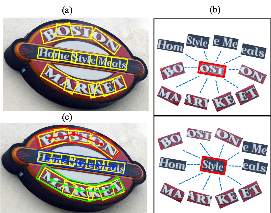
Figure 1: Illustration of the proposed framework, best viewed in color. Firstly, the oriented text segments (yellow rectangles in (a) ) are detected, some cases are skipped for better visualization. Then, each segment plays as an anchor (highlighted by red borders in (b)) to be extracted correlations (blue dotted lines in (b)) between itself and its contextual ones. Finally, the combinations between adjacent segment pairs are predicted (same-combination segments are connected by the same color solid lines in (c)). According to the predicted combinations, segments are merged into the final detection results (depicted in polygons of different colors in (c)).

Alternatively, one category of prevalent methods is decomposition-based methods [27, 10, 24, 1, 5, 32], which handle challenging texts by decomposing them into pieces and linking those belonging to the same text region in a bottom-up manner. However, most of these previous methods simply focus on linking individual text pieces while the context information of each text piece is not given sufficient attention. In real situations, people are likely to judge whether two text pieces belong to the same text region according to their context information (e.g., character layout or font), rather than the limited information carried by two individual pieces themselves. This is similar to puzzle game, in which the solver put pieces together according to the patterns and particular ordering of contextual pieces, in order to arrive at the correct solution.

Inspired by above observations, we propose a novel decomposition-based scene text detection architecture, named Puzzle Networks (PuzzleNet). The overview of the proposed framework is illustrated in Fig. 1. We decompose arbitrary-shape text region into a number of text pieces represented by segments. Here, a segment refers to an oriented rectangle (yellow rectangle in (a)) covering a part of the text region. Then each segment is regarded as an anchor (highlighted by red borders in (b)) to model the interior correlations (blue dotted lines in (b)) between it and contextual segments. Then segments are merged together to form the final detection results (polygons of different colors in (c)) according to the predicted combinations (same-combination segments are connected by the same color solid lines in (c)). Here, segments from the same text region are deemed in a correct combination.

The above text detection procedure involves two non-trivial problems: 1) predicting high-quality candidate text segments for the following context construction; 2) integrating correlations between each segment and contextual ones into combination prediction procedure.

Most of previous works [24, 10, 1, 5, 32] represent text pieces as orientated square boxes or character boxes. This type of representation has a main drawback that the covering region of each independent box is too limited to provide sufficient information for linking independent box pairs together. Moreover, we observe that the adjacent characters in a local region often have similar orientations, though different characters in curved shape text have different orientations. Take the curved-line text “BOSTON” in Fig. 1(a) for example, the region of “BO” has an approximately same orientation while the region of “OST” has another one. Therefore, in this work we propose to represent text piece by rectangular segment covering larger local text region with more effective information. Instead of greedily predicting orientated square box at every position of text region, a more effective way is to predict the fewer number of segments covering text regions with similar orientations. To achieve this goal, we propose the local orientation aware Segment Proposal Network (SPN) to detect segments.

The remaining question is how to make full use of segments and their context to predict their combinations. We propose to construct segments as context graphs, in which each node corresponds to a segment. Correlations between segments are represented by edges. In this way, each segment can be either an anchor or one of context to others simultaneously. Aiming at inferring combinations of each adjacent pairwise segments, we coin the innovative two-branch Graph Convolution Network (GCN) to perform reasoning on segment context graphs from both appearance and geometry perspectives. Furthermore, we extend GCN to the Multiple-Similarity GCN (MSGCN) by introducing multiple-similarity mechanism to better capture the appearance and geometry correlations between segments. In the end, corresponding segments belonging to the same combination are grouped into several clusters and merged to form the polygon shape of detection results.

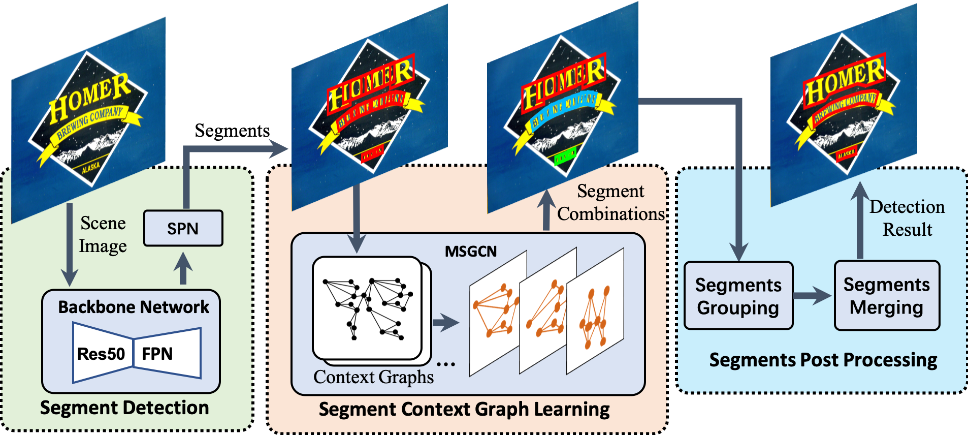
Figure 2: The overview of our proposed Puzzle Networks (PuzzleNet). Given a scene image, the network outputs text segments and segment combinations by segment detection and Multiple-Similarity Graph Convolutional Network (MSGCN). Finally, detection result is generated by grouping and merging segments. Best viewed in color.

Our contributions are in the following three folds: 1) A novel scene text detector named PuzzleNet is proposed, which is flexible for text instance with arbitrary shape, orientation and varying aspect ratio. 2) A local orientation aware SPN is designed to predict the segments with more effective representation of text regions. 3) To our best knowledge, we are the first to build segments as context graphs and learn their correlations considering context information for predicting their combinations. We evaluate our approach on three public benchmarks, ICDAR15, MSRA-TD500 and SCUT-CTW1500. Experimental results demonstrate that our method is able to achieve significantly better performance compared with state-of-the-arts.

2 Related Work

With the development of deep learning, scene text detection has recently advanced substantially on both performance and robustness. The deep learning-based scene detection methods can be roughly categorized into three groups: regression-based, segmentation-based and decomposition-based methods.

Regression-based methods [15, 38, 22, 16] aims to design the robust generation method of bounding box to improve the performance. TextBoxes [15] introduce long default boxes and convolutional filters to cope with the long aspect ratio text lines. In [22], the Rotation Region Proposal Networks (RRPN) are designed to generate inclined proposals with text orientation angle information. Besides, Liao et al.[16] propose to perform classification and regression on features of different characteristics with a two-branch model. However, these methods are still disturbed by the large aspect ratio variations and irregular shape of the text region.

Segmentaion-based methods [34, 4, 20, 28, 31, 37] regard all the pixels within text bounding boxes as positive regions and directly draw text bounding boxes from predicted segmentation map. Pixellink [4] predicts instance-segmentation map and linking pixels within the same instance together. However, this method is liable to failure when two text lines lie close to each other. Recent work [21] introduce position-sensitive segmentation to solve the problem. But it can only handle the rectangular shape text region. Textsnake [20], PSENet [28] , LOMO [37] and SPCNET [31] predict text center line map to separate different text instances, whose performance strongly affected by the robustness of segmentation results.

Decomposition-based methods [27, 10, 26, 24, 1, 5, 32] first decompose text region into pieces or characters, and then group them into final detection results. Our method belongs to this category which can essentially well handle the text cases with arbitrary shape, orientation and aspect ratio. Among the recent methods, CTPN [27] generates dense and compact text components. In character level, WordSup [10], Wetext [26] and CRAFT [1] propose to localize individual characters in the image and group them into a single instance. Although introducing weakly supervised learning, these methods still need strict character level annotations.

Particularly, different from SegLink [24] using the square shape segment, our method focuses on detecting the arbitrary-shape text and predicting rectangular segments which carry more effective information. Comparatively, SegLink can only detect the text in line shape by predicting square boxes. Besides, all above mentioned decomposition-based methods only exploit the information carried by individual text piece pairs themselves when predicting the relationship or affinity between them, in which context information of text pieces, such as character layout structure, is not fully utilized. Contrastively, our proposed PuzzleNet can capture and aggregate the context information of segments by building segment context graphs to facilitate the prediction of their combinations.

3 Proposed Puzzle Networks

The overview of the proposed Puzzle Networks (PuzzleNet) is shown in Fig. 2. It consists of three components, i.e., segment detection, segment context graph learning and segment post processing. First, segments are predicted based on the proposed local orientation aware Segment Proposal Network (SPN). After building them as context graphs, we perform reasoning on graphs via the newly proposed Multiple-Similarity Graph Convolutional Network (MSGCN) to predict segment combinations. Finally, the segments are grouped into several clusters according to the predicted combinations, and then the segments in the same cluster are merged as the final detection result.

3.1 Backbone Network

Our method adopts ResNet [7] of 50 layers with a Feature Pyramid Network (FPN) [17] as the backbone network (illustrated in green part of Fig. 2). For a single-scale input scene image, FPN utilizes a top-down architecture with lateral connections to build an feature pyramid from it. Features output by last residual blocks of conv2, conv3, conv4 and conv5 are denoted as {$C_{2}$, $C_{3}$, $C_{4}$, $C_{5}$}, which respectively have strides of {4, 8, 16, 32} pixels with respect to the input image. Correspondingly, a set of upsampled features output by FPN is called {$P_{2}$, $P_{3}$, $P_{4}$, $P_{5}$}. Note, slightly different from the vanilla ResNet50-FPN in [17], we insert non-local blocks proposed in [29] after $C_{2}$ and $C_{4}$ to capture long range dependencies, which can model interactions between any two pixels, regardless of their positional distance.

3.2 Segment Detection

As discussed, our method first detects a set of segments satisfying that local adjacent text regions with a similar orientation covered by a rectangular segment. To this end, we design the local orientation aware Segment Proposal Network (SPN) and generate the Ground Truth (GT) segment from GT polygon for training it. In our method, the segment is denoted as $\textit{S}=(x,y,w,h,\theta)$, where $(x,y)$ is the center point of segment while height $h$ and width $w$ correspond to its short side and long side respectively. $\theta$ represents the angle measured counter-clockwise from the positive x-axis.

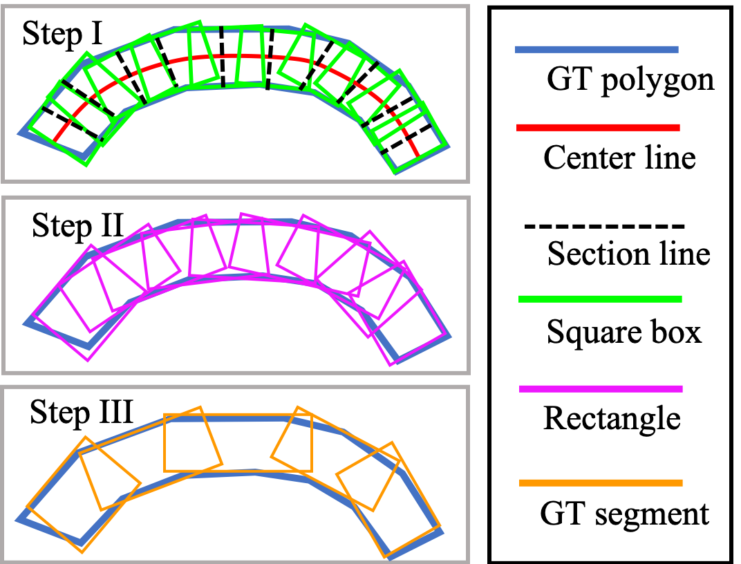
Figure 3: Illustration of ground truth (GT) segment generation. The procedure of generation includes three steps: I. Extracting text center line and generating square boxes covering GT polygon; II. Merging square boxes into rectangles; III. Merging rectangles with similar orientations into GT segments. Best viewed in color.

Ground Truth Segment Generation We first elaborate on how to generate Ground Truth (GT) segment from GT polygon as supervision. More concretely, we decompose the GT polygon into several GT segments in three steps, which is illustrated in Fig. 3. It is easy to directly decompose rectangular box into segments. However, decomposition on polygons of more than 4 sides is not easy with a general algebraic method. Therefore, we firstly adopt the method in [20] to generate the text center line (red solid line in Fig. 3) of polygon (depicted in dark blue in Fig. 3) . Then the center line is evenly sectioned into $n$ line segments by $n-1$ section points. We set $n$ to 50 in this paper. The interval $\tau$ is determined by the following equation:

$$\small\tau=\sigma\cdot\min(\{\|l^{cross}_{i}\|\}),i=1,2,...,n-1.$$ (1)

And $\|l^{cross}_{i}\|$ denotes the length of $i$-th cross section line (doted line in Fig. 3) at $i$-th sample point. $\sigma$ is the scale coefficient which is set to 0.5. Then, each cross section line plays as the axis to generate a square box (green box in Fig. 3) covering part of polygon. The side length of the square box equals to the length of corresponding cross section line. In the second step, each two neighbouring square boxes are merged into a rectangle (magenta boxes in Fig. 5) by calculating the enclosing rectangle of region covered by two square boxes. In the final step, those adjacent rectangles with angle difference smaller than $\pi/36$ are further merged into longer ones as GT segments (orange boxes in Fig. 3) if the aspect ratios of them suffice to smaller than 3. By this way, the GT segments with local similar orientations are generated.

Segment Proposal Network The detailed structure of Segment Proposal Network (SPN) is depicted in Fig. 4, which is derived from Rotation Region Proposal Network (RRPN) [22]. To expediently detect segment, in SPN we use 4 scale anchors of $\{32^{2},64^{2},128^{2},256^{2}\}$ with multiple orientations ${\{-\pi/6,0,\pi/6,\pi/3,\pi/2,2\pi/3\}}$ on {$P_{2}$, $P_{3}$, $P_{4}$, $P_{5}$} respectively. The aspect ratios are set to $\{1.5,2,2.5\}$. Further, we assign RRoIs of different sizes to different pyramid levels with different scales. The assign rule inherits from [17]. Besides, instead of using RRoI pooling [22], we apply RRoI Align [11] on different level RRoIs to avoid misaligned results. The features of $7\times 7\times d$ size output by RRoI Align are then sent to two Fully-Connected (FC) layers with 512 dimensions. The segment score and coordination regression are then performed via linear layers.

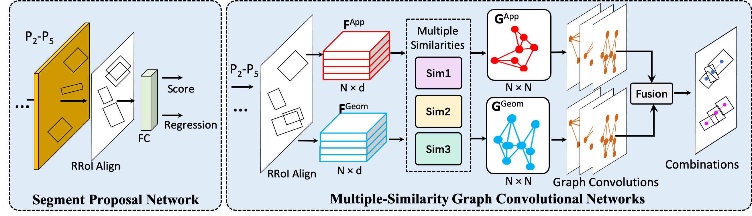
Figure 4: The detailed network of Segment Proposal network(SPN) and Multiple-Similarity Graph Convolutional Network (MSGCN). Best viewed in color.

3.3 Segment Context Graph Learning

In this section, we introduce the detailed structure of the proposed segment context graph as well as the Multiple-Similarity Graph Convolutional Network (MSGCN) to learn graph parameters. The details is illustrated in Fig. 4.

Multiple-Similarity Graph Convolutional Network Given a set of segments, the objective of MSGCN is to construct them as graphs to jointly take the segments and their context information into consideration, and judge whether segment pairs belong to the same combination.

We observe that segments belonging to the same combination often have similar appearance (e.g., character font) and their layouts have certain natural graph structures. Therefore, we construct segments as graphs from both appearance and geometry perspectives. In the constructed graphs, each segment can be either an anchor or one of context of others. In particular, we first extract their appearance feature and geometry feature as nodes to construct graphs.

To extract appearance feature, the RRoI Align is applied on corresponding pyramid level in the similar way with segment detection stage. Three convolutional layers with $3\times 3\times 512$ size of kernel are then applied. We denote the segment number as $N$. After passing a FC layer with $d$ dimensions, appearance features $\mathbf{F}^{\text{App}}=\left\{\mathbf{f}_{1},\mathbf{f}_{2},...,\mathbf{f}_{N}\right\}\in\mathbb{R}^{N\times d}$ are obtained, as depicted in red cubes in Fig. 4.

Basing on the segment denotion in Sec. 3.2, we derive the geometry feature of each segment as $\left({\frac{x}{W}},{\frac{y}{H}},{\frac{w}{W}},{\frac{h}{H}},\theta\right)^{\top}$, where $W$ and $H$ are the width and height of the scene image. Then a $d$-dimension FC is applied on above vectors to obtain the geometry features $\mathbf{F}^{\text{Geom}}=\left\{\mathbf{g}_{1},\mathbf{g}_{2},...,\mathbf{g}_{N}\right\}\in\mathbb{R}^{N\times d}$, which described in blue cubes in Fig. 4.

Then, two kinds of nodes are connected by two types of edges separately: appearance similarity and geometry similarity. With similarity relations, we can model the interplay of appearance and geometry between each segment and its contexts. The appearance similarity $\mathbf{G}^{\text{App}}$ (red graph in Fig. 4) and geometry similarity $\mathbf{G}^{\text{Geom}}$ (blue graph in Fig. 4) can be computed as

$$\mathbf{G}_{i,j}^{\text{App}}=K(\mathbf{f}_{i},\mathbf{f}_{j}),i,j\in\{1,2,...,N\},$$ (2)

$$\mathbf{G}_{i,j}^{\text{Geom}}=K(\mathbf{g}_{i},\mathbf{g}_{j}),i,j\in\{1,2,...,N\},$$ (3)

where $K$ is the similarity function. To better capture the correlations between segment pairs, we equip it with three types of similarities, which can be represented as

$$K=\beta_{1}K_{1}+\beta_{2}K_{2}+\beta_{3}K_{3},\text{s.t. }\beta_{1}+\beta_{2}+\beta_{3}=1,$$ (4)

$$K_{1}(\textbf{y}_{1},\textbf{y}_{2})=\frac{\textbf{y}_{1}\cdot\textbf{y}_{2}^{\top}}{(\left|\textbf{y}_{1}\right|\cdot\left|\textbf{y}_{2}\right|)},$$ (5)

$$K_{2}(\textbf{y}_{1},\textbf{y}_{2})=\exp(-\frac{\left\|\textbf{y}_{1}-\textbf{y}_{2}\right\|^{2}}{2\sigma^{2}}),$$ (6)

$$K_{3}(\textbf{y}_{1},\textbf{y}_{2})=\exp(-\frac{\textit{JSD}(\textbf{y}_{1},\textbf{y}_{2})}{2\sigma^{2}}),$$ (7)

$$\textbf{y}_{1}=\phi_{1}(\textbf{x}_{1})=\textbf{w}_{1}\textbf{x}_{1},\quad\textbf{y}_{2}=\phi_{1}(\textbf{x}_{2})=\textbf{w}_{2}\textbf{x}_{2}.$$ (8)

$K_{1}$, $K_{2}$ and $K_{3}$ are cosine similarity, Gaussian similarity and Jensen-Shannon similarity [2] respectively. JSD represents the Jensen-Shannon Divergence and $\sigma$ is the control parameter set to 5 in this work. $(\beta_{1},\beta_{2},\beta_{3})$ are similarity weight parameters which can be learned through back propagation. $\phi_{1}$ and $\phi_{2}$ represents two different transformations of the input features $\textbf{x}_{1}$ and $\textbf{x}_{2}$. The parameters $\textbf{w}_{1}$ and $\textbf{w}_{2}$ are both $d\times d$ dimensions weights which can be learned via back propagation. Note, $\mathbf{G}^{\text{App}}$ and $\mathbf{G}^{\text{Geom}}$ are produced by passing $\mathbf{F}^{\text{App}}$ and $\mathbf{F}^{\text{Geom}}$ through $K$ individually. By introducing multiple-similarity mechanism to our graph reasoning model, it enables more effective message passing between each node. It also provides significant boost to the performance of our scene text detection task which will be verified by analytic experiments in Sec. 5.3. Then the $\mathbf{G}^{\text{App}}$ and $\mathbf{G}^{\text{Geom}}$ are adopted as the adjacency matrix representing the similarity graphs in our work.

To perform reasoning on context graphs, the Graph Convolutional Network (GCN) [14] is applied. Formally, one basic layer of graph convolutions can be represented as $\mathbf{Y}=\mathbf{G}\mathbf{X}\mathbf{W}$, where $\mathbf{G}\in\mathbb{R}^{N\times N}$ is the adjacency matrix we have introduced above ($\mathbf{G}^{\text{App}}$ or $\mathbf{G}^{\text{Geom}}$), $\mathbf{X}\in\mathbb{R}^{N\times d}$ is the input features, $\mathbf{W}$ represents the $d\times d$-dimension weight matrix while $\mathbf{Y}\in\mathbb{R}^{N\times d}$ denotes the output features. To make the information flow unimpeded, we equip every layer of GCN with a residual connection in our method. Then the graph convolutional layer can be extended as $\mathbf{Y}=\mathbf{G}\mathbf{X}\mathbf{W}+\mathbf{X}.$

Then, the Layer Normalization and ReLu layers are applied on the output of each layer. In this work, we apply two branches of 3-layer GCN on $\mathbf{G}^{\text{App}}$ and $\mathbf{G}^{\text{Geom}}$ individually, as illustrated in the Fig. 4. After that, the outputs of two branches are fused by concatenating them into the feature in $N\times 2d$ dimensions. To predict final combination scores of each pairwise nodes, we apply two $N$-dimension FC layers and a convolutional layer with $1\times 1\times 2$ kernel size on the fused feature to obtain the feature map in $N\times N\times 2$ dimensions. In the end, the position-wise softmax function is performed on it to get the final combination score map $\mathbf{C}$. The score $s_{i,j}\in\mathbf{C}$ indicates the probability of $i$-th segment and $j$-th segment belonging to the same combination.

3.4 Segment Post Processing

After segments and corresponding combination score maps obtained, two steps of post processing should be performed to output the final detection results, as shown in Fig. 2.

Segment Grouping The first step is grouping candidate segments into different clusters according to the combination score maps. Our model infers the combinations of the adjacent segment pairs. To construct pairs, we exploit k-Nearest Neighbors with Radius (kNNR) [35] algorithm for each segment. For $m$-th segment $S_{m}$, its adjacent pair segments $S_{n}\in\mathbf{S}^{\text{adj}}$ should subject to the following two rules: (1) $S_{n}$ are in the set of k-Nearest Neighbors, which are determined by the Euclidean distance of their centers $D_{m,n}=\sqrt{(x_{m}-x_{n})^{2}+(y_{m}-y_{n})^{2}}$; (2) $D_{m,n}<R$, where $R$ is the radius computed as $R=\alpha\sqrt{w_{m}^{2}+h_{m}^{2}}$. In this work, $k$ and $\alpha$ are set to 5 and 2.5 respectively. Then, for each segment $S_{m}$, its matchable segment $\hat{S}$ (linked by the same color lines in Fig. 1) should satisfy that $\hat{s}=max(\mathbf{C}^{\text{adj}})$ and $\hat{s}>0.5$, where $\hat{s}$ is the combination score of $\hat{S}$. Through this way, all segments can be grouped into several clusters. As is shown in Fig.2, three clusters of segments are represented in red, blue and green respectively.

Segment Merging In each cluster, we firstly generate segment bisection line (black dotted line in Fig. 5) of each segment along short side direction, then the angle between two neighbouring center lines are evenly divided by a bisection line (red dotted line in Fig. 5). After that, the vertices on the closest short sides of two segments are extracted, denoted as $\{{v^{(e)}_{f}}\},e,f\in\{1,2\}$, where $e$ stands for the $e$-th segment and $f$ is the $f$-th vertex. Correspondingly, we project the vertices on the angle bisection line and two projected points with max distance are kept. Their corresponding vertices are regarded as contour points(red points in Fig. 5). Note, if two segments have the same angle, the center line of any one of them is deemed as bisection line. Finally, the contour points are connected along the direction of segment long side. To make the boundary curve of final detection more smooth, a thin plate spline (TPS) [3] method is applied.

4 Training Strategy

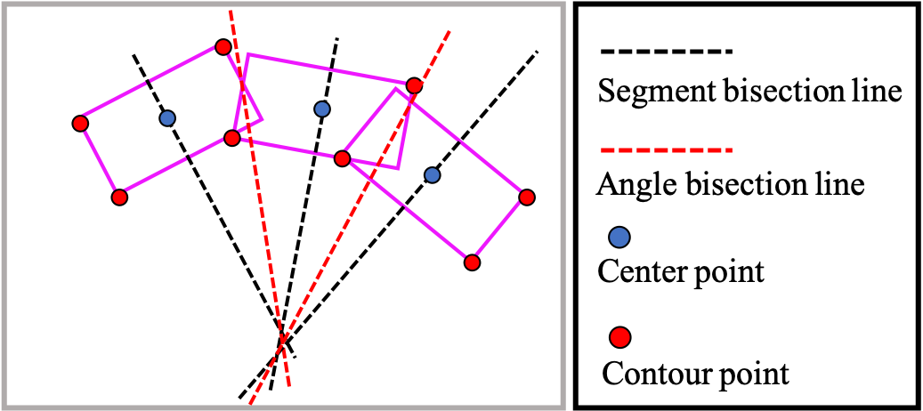
Figure 5: Illustration of segment merging procedure. Best viewed in color.

We train our proposed PuzzleNet in an end-to-end way. And the multi-task loss function is defined as

$$\small L=L_{reg}+\lambda_{1}L_{score}+\lambda_{2}L_{comb},$$ (9)

where $L_{reg}$ and $L_{score}$ are the loss functions of SPN while $L_{comb}$ is the “combination” loss of combination prediction in MSGCN. $\lambda_{1}$ and $\lambda_{2}$ are the weights constants to control the trade-off of three terms. In default, we set the $\lambda_{1}$ and $\lambda_{2}$ to 1 and 5. We regress the predicted tuple of text label $\mathbf{v}=(v_{x},v_{y},v_{w},v_{h},v_{\theta})$ to the GT segment (introduced in Sec. 3.2) $\mathbf{\hat{v}}=(\hat{v}_{x},\hat{v}_{y},\hat{v}_{w},\hat{v}_{h},\hat{v}_{\theta})$:

$$\small L_{reg}=SmoothedL1(\mathbf{\hat{v}},\mathbf{v}).$$ (10)

Besides, Cross Entropy loss is adopted as $L_{score}$ to train the classifier of SPN in segment detection stage.

Given $N$ segments, we generate the position-wise combination label map $\mathbf{U}$ of $N\times N$ size for “combination” loss. The combination score for position $(p,q)$ can be defined as

$$\small U_{p,q}=\begin{cases}\textbf{1},\text{if }P=Q\text{ and }S^{(Q)}_{q}\in\textit{kNNR}(S^{(P)}_{p})\\ \textbf{0},\text{otherwise},\\ \end{cases}$$ (11)

where $S^{(P)}$ and $S^{(Q)}$ represent segments belong to $P$-th and $Q$-th GT polygons. Specifically, if $area(Segment\cap Polygon)/area(Segment)>0.8$, the segment is deemed belong to the GT polygon. $\textit{kNNR}(S^{(P)}_{p})$ denotes a set of adjacent segment pairs to the segment $S^{(P)}_{p}$ after kNNR applied. Taking $\mathbf{U}$ as supervision, the position-wise softmax loss is adopted to compute “combination” loss $L_{comb}$ between $\mathbf{U}$ and the output feature of last layer of MSGCN. Note, the combination loss at position $(p,q)$ would be ignored if $p$ = $q$ because the relationship between segment and itself is deterministic.

5 Experiments

5.1 Datasets

SynthText  [6] is a large scale dataset containing round 800,000 synthetic images. This dataset is utilized to pre-train our model.

MSRA-TD500 [33] is a dataset collected for detecting long text lines of arbitrary orientations with text line level annotations. It contains 300 images for training and the remaining 200 images constitute the test set.

ICDAR2015 is a dataset proposed as the Challenge 4 of the 2015 Robust Reading Competition [12] for incidental scene text detection. It consists of 1,000 training images and 500 test images with word level annotations of the quadrangle.

SCUT-CTW1500 [36] is a challenging dataset collect for detecting curved text. It consists of 1,000 images for training and 500 images for testing, which are labelled by a polygon with 14 points.

5.2 Implementation Details

Our method is implemented in Pytorch [23]. The network is pre-trained on SynthText for one epoch and fine-tuned on other datasets. Adam [13] optimizer is adopted for our method, and the learning rate is set to $1e-4$. We use the OHEM proposed in [25] in training stage to balance training samples and set the ratio of positives to negatives to 1:2. Considering computation cost would be huge if MSGCN takes all segments as input nodes, we apply the Skew-NMS[22] after segment detection in both training and inference stage. The threshold of Skew-IoU and angle difference are set to 0.7 and $\pi/36$ respectively. For data augmentation, we randomly rotate the input images in a certain angle ranging from $-\pi/12$ to $\pi/12$. Other augmentation tricks, e.g., randomly modifying hue , brightness and contrast, are also adopted. All the experiments are conducted on a regular platform with 8 Nvidia P40 GPUs and 64GB memory. We train our network in batch size of 2 and set it to 1 when evaluating.

5.3 Ablation Study

Table 1: Results of ablation study on SCUT-CTW1500. “w/o App”, “w/o Geom” and “w/o Graph” are short for “without appearance”, “without geometry” and“without graph”, respectively.

Method	Precision	Recall	F-measure
PuzzleNet w/o App	73.4	78.0	75.7
PuzzleNet w/o Geom	69.2	72.5	70.8
PuzzleNet w/o Graph	65.7	69.0	67.3
PuzzleNet-SSim	80.3	83.8	82.0
PuzzleNet-Square	73.4	78.0	75.7
PuzzleNet-MS	83.3	86.5	84.9
PuzzleNet	84.1	84.7	84.4

In this subsection, we perform several analytic experiments on SCUT-CTW1500 benchmark to verify the effectiveness of our proposed PuzzleNet architecture. We analyze and investigate the effect of several factors upon the performance, which mainly include context graph mechanism, segment type and multi-scale input. In total we have six variants by training the model based on different combinations of the above factors. In all the experiments using single-scale image as input, the long side of input image is set to 800. And fine-tuning on stops at about 100 epochs. The details and corresponding results are shown in Tab. 1.

Effect of Context Graph In the method “PuzzleNet w/o App”, we remove the “appearance” branch. Now, the module can only capture and exploit the geometry information of segment context to predict their combinations. We observe the F-measure score drops 8.7%. Comparatively, if we remove the “geometry” branch in “PuzzleNet w/o Geom” method, we find this setting would be more detrimental to the performance. In method named “PuzzleNet w/o Graph”, we completely remove the MSGCN and use three $d$-dimension FC layers instead. For combination prediction, we concatenate appearance and geometry features and compute their Euclidean distance. Under this condition, the graph-based correlation reasoning mechanism is completely removed, we find that simply using appearance and geometry features can not achieve satisfactory results. By comparing the results between “PuzzleNet” and “PuzzleNet-SSim” which only adopts single cosine similarity function to build graphs, we observe that the “PuzzleNet” achieves higher performance due to its ability of ensemble multiple source information from different similarity spaces. From the result “PuzzleNet” overtaking above four degraded PuzzleNets by a large margin for all three evaluation protocols, we come to the conclusion that the segment context graph learning mechanism is beneficial to scene text detection performance.

In Fig. 6, for an image from SCUT-CTW1500, we visualize the results output by appearance and geometry similarity modules formulated by Eqn. (2) and Eqn. (3), which indicate the appearance and geometry contributions of context in combination prediction. For a certain anchor segment (green), its three contextual samples with largest appearance similarities which larger than 0.5 are highlighted in red in Fig. 6(b). We observe that they have similar appearance, such as font or background. As to the contextual samples (blue ones in Fig. 6(c))with largest geometry similarities which larger than 0.5, we find they locate near the anchor segment, which is reasonable. The above phenomena further demonstrate that our method can extract and aggregate effective context information by a graph model for text detection task. In addition, the generated contour points introduced in Sec. 3.4 and linked polygons are also visualized in Fig. 6(d).

Table 2: Results on ICDAR2015.

Method	Precision	Recall	F-measure
SegLink [24]	73.1	76.8	75.0
PixelLink [4]	85.5	82.0	83.7
Lyu et al.[21]	89.5	79.7	84.3
EAST [38]	83.3	78.3	80.7
SSTD [8]	80.0	73.0	77.0
He et al. [9]	82.0	80.0	81.0
TextSnake [20]	84.9	80.4	82.6
SPCNET [31]	88.7	85.8	87.2
Wang et al. [30]	89.2	86.0	87.6
CRAFT [1]	89.8	84.3	86.9
PSENet [28]	86.9	84.5	85.7
FOTS [18]	88.8	82.0	85.3
CharNet [32]	90.2	81.4	85.6
TextDragon [5]	84.8	81.8	83.1
LOMO [37]	91.3	83.5	87.2
LOMO MS [37]	87.8	87.6	87.7
PuzzleNet	89.1	86.9	88.0
PuzzleNet-MS	88.9	88.1	88.5

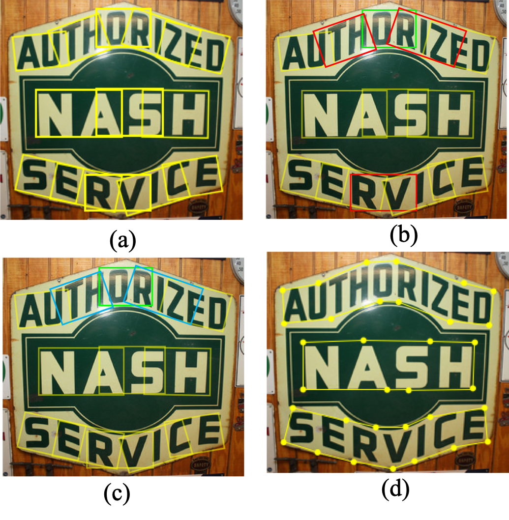
Figure 6: (a) showing the segments predicted by SPN. (b) and (c) respectively showing the contextual samples (red) with largest appearance similarities and the contextual samples (blue) with largest geometry similarity to the anchor segment (green). Transparent purple segments are the other ones. (d) showing the generated contour points (yellow points) and the linked polygons.

Effect of Segment Type In the method “PuzzleNet-Square”, we replace the segment representation with the square box used in SegLink [24]. The comparison results between it and “PuzzleNet” verify the local orientation aware rectangular segments can provide more effective information for constructing context graph and achieving higher performance.

Effect of Multi-scale input By using multi-scale images as input, our PuzzleNet can achieve better recall rate and F-measure, as shown by “PuzzleNet-MS”. In the multi-scale setting, the long side of images is resize to $\{400,600,800,1000\}$. It demonstrates that multi-scale input could produce more effective segments and our method is capable to combine them in the correct way.

5.4 Comparison with State-of-the-Art Methods

Results on ICDAR2015 We fine-tune our network on ICDAR2015 in 400 epochs. In single-scale testing, we resize the longer side of input image to 1536. And the longer sides in multi-scale testing are set to $\{1024,1536,2048\}$. The comparison of our method’s performance with different state-of-the-arts on ICDAR 2015 are shown in Tab. 2. With only single-scale testing, our method outperforms most previous methods by a large margin. Specifically, our PuzzleNet can achieve the F-measure of 88.0%, which surpasses the LOMO MS [37] with multi-scale input. This demonstrates that our proposed PuzzleNet is capable to effectively detect multi-oriented text in complex scenarios.

Table 3: Results on MSRA-TD500.

Method	Precision	Recall	F-measure
SegLink [24]	86.0	70.0	77.0
Lyu et al. [21]	87.6	76.2	81.5
EAST [38]	87.3	67.4	76.1
He et al. [9]	77.0	70.0	74.0
TextSnake [20]	83.2	73.9	78.3
PixelLink [4]	83.0	73.2	77.8
Wang et al. [30]	85.2	82.1	83.6
CRAFT [1]	88.2	78.2	82.9
PuzzleNet	88.2	83.5	85.8
PuzzleNet-MS	86.0	86.2	86.1

Results on MSRA-TD500 To further evaluate the performance of our method for detecting long oriented text lines with multi languages, we conduct experiments on MSRA-TD500. After pre-trained on SynthText, our model is fine-tuned in 300 epochs. In testing, all images are resized to $1280\times 768$. The quantitative results are shown in Tab. 3. Our method surpasses all the other methods by a large margin and achieves 2.2% gain for F-measure protocol. The results suggest that our method can be readily applied to long text lines with arbitrary orientations in natural images.

Results on SCUT-CTW1500 As shown in Tab. 4, “PuzzleNet” using single-scale input image can achieve 84.4% of the best F-measure compared to other methods. Although LOMO [37] can achieve the best precision, our method overtakes it by 15.1% for recall protocol. “PuzzleNet-MS” adopting multi-scale image can further boost the recall to 86.5%. The superior performance verifies our method can handle well curved scene text.

Table 4: Results on SCUT-CTW1500.

Method	Precision	Recall	F-measure
SegLink [24]	42.3	40.0	40.8
EAST [38]	78.7	49.1	60.4
TextSnake [20]	67.9	85.3	75.6
CTD [36]	74.3	65.2	69.5
CTD+TLOC [36]	77.4	69.8	73.4
CTPN [27]	60.4	53.8	56.9
DMPNet [19]	69.9	56.0	62.2
Wang et al. [30]	80.1	80.1	80.2
CRAFT [1]	86.0	81.1	83.5
PSENet [28]	84.8	79.7	82.2
TextDragon [5]	84.5	82.8	83.6
LOMO [37]	89.2	69.6	78.4
LOMO MS [37]	85.7	76.5	80.8
PuzzleNet	84.1	84.7	84.4
PuzzleNet-MS	83.3	86.5	84.9

5.5 Detected Examples on Benchmark Datasets

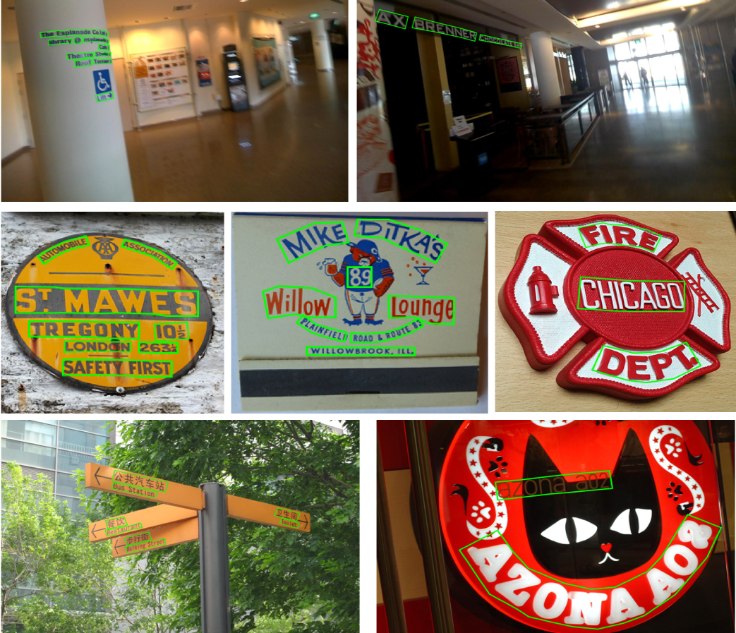
Figure 7: Examples of detection results. From top to bottom in rows: ICDAR2015, SCUT-CTW1500, MSRA-TD500

In Fig. 7, we also visualize detection results produced by our PuzzleNet for testing samples from ICDAR2015, SCUT-CTW1500 and MSRA-TD500 dataset. The first row is from ICDAR2015, while the second and third rows are from SCUT-CTW1500 and MSRA-TD500 respectively. We observe that our detection model can predict precise description of the shape and course of text instances with arbitrary orientations and shapes. We attribute such ability to the segment context graph learning mechanism.

6 Conclusions

We present a novel decomposition-based method solves scene text detection through learning segment context graph. Extensive experiments on three public benchmarks demonstrate its superiority over state-of-the-art methods in most cases in scene text detection.

References

- [1] Youngmin Baek, Bado Lee, Dongyoon Han, Sangdoo Yun, and Hwalsuk Lee. Character region awareness for text detection. In IEEE CVPR, 2019.
- [2] Lu Bai and Edwin R Hancock. Graph kernels from the jensen-shannon divergence. Journal of mathematical imaging and vision, 47(1-2):60–69, 2013.
- [3] Fred L. Bookstein. Principal warps: Thin-plate splines and the decomposition of deformations. 11(6):567–585, 1989.
- [4] Dan Deng, Haifeng Liu, Xuelong Li, and Deng Cai. Pixellink: Detecting scene text via instance segmentation. In AAAI, 2018.
- [5] Wei Feng, Wenhao He, Fei Yin, Xu-Yao Zhang, and Cheng-Lin Liu. Textdragon: An end-to-end framework for arbitrary shaped text spotting. In The IEEE International Conference on Computer Vision (ICCV), October 2019.
- [6] Ankush Gupta, Andrea Vedaldi, and Andrew Zisserman. Synthetic data for text localisation in natural images. In IEEE CVPR, 2016.
- [7] Kaiming He, Xiangyu Zhang, Shaoqing Ren, and Jian Sun. Deep residual learning for image recognition. In IEEE CVPR, pages 770–778, 2016.
- [8] Pan He, Weilin Huang, Tong He, Qile Zhu, Yu Qiao, and Xiaolin Li. Single shot text detector with regional attention. In IEEE ICCV, pages 3047–3055, 2017.
- [9] Wenhao He, Xu-Yao Zhang, Fei Yin, and Cheng-Lin Liu. Deep direct regression for multi-oriented scene text detection. In IEEE ICCV, pages 745–753, 2017.
- [10] Han Hu, Chengquan Zhang, Yuxuan Luo, Yuzhuo Wang, Junyu Han, and Errui Ding. Wordsup: Exploiting word annotations for character based text detection. In IEEE ICCV, pages 4940–4949, 2017.
- [11] Jing Huang, Viswanath Sivakumar, Mher Mnatsakanyan, and Guan Pang. Improving rotated text detection with rotation region proposal networks. arXiv preprint arXiv:1811.07031, 2018.
- [12] Dimosthenis Karatzas, Lluis Gomez-Bigorda, Anguelos Nicolaou, Suman Ghosh, Andrew Bagdanov, Masakazu Iwamura, Jiri Matas, Lukas Neumann, Vijay Ramaseshan Chandrasekhar, Shijian Lu, et al. Icdar 2015 competition on robust reading. In ICDAR, pages 1156–1160, 2015.
- [13] Diederik P Kingma and Jimmy Ba. Adam: A method for stochastic optimization. arXiv preprint arXiv:1412.6980, 2014.
- [14] Thomas N Kipf and Max Welling. Semi-supervised classification with graph convolutional networks. arXiv preprint arXiv:1609.02907, 2016.
- [15] Minghui Liao, Baoguang Shi, Xiang Bai, Xinggang Wang, and Wenyu Liu. Textboxes: A fast text detector with a single deep neural network. In AAAI, 2017.
- [16] Minghui Liao, Zhen Zhu, Baoguang Shi, Gui-song Xia, and Xiang Bai. Rotation-sensitive regression for oriented scene text detection. In IEEE CVPR, pages 5909–5918, 2018.
- [17] Tsung-Yi Lin, Piotr Dollár, Ross Girshick, Kaiming He, Bharath Hariharan, and Serge Belongie. Feature pyramid networks for object detection. In IEEE CVPR, pages 2117–2125, 2017.
- [18] Xuebo Liu, Ding Liang, Shi Yan, Dagui Chen, Yu Qiao, and Junjie Yan. Fots: Fast oriented text spotting with a unified network. In IEEE CVPR, pages 5676–5685, 2018.
- [19] Yuliang Liu and Lianwen Jin. Deep matching prior network: Toward tighter multi-oriented text detection. In IEEE CVPR, pages 1962–1969, 2017.
- [20] Shangbang Long, Jiaqiang Ruan, Wenjie Zhang, Xin He, Wenhao Wu, and Cong Yao. Textsnake: A flexible representation for detecting text of arbitrary shapes. In ECCV, pages 20–36, 2018.
- [21] Pengyuan Lyu, Cong Yao, Wenhao Wu, Shuicheng Yan, and Xiang Bai. Multi-oriented scene text detection via corner localization and region segmentation. In IEEE CVPR, pages 7553–7563, 2018.
- [22] Jianqi Ma, Weiyuan Shao, Hao Ye, Li Wang, Hong Wang, Yingbin Zheng, and Xiangyang Xue. Arbitrary-oriented scene text detection via rotation proposals. IEEE TMM, 20(11):3111–3122, 2018.
- [23] Adam Paszke, Sam Gross, Soumith Chintala, Gregory Chanan, Edward Yang, Zachary DeVito, Zeming Lin, Alban Desmaison, Luca Antiga, and Adam Lerer. Automatic differentiation in pytorch. 2017.
- [24] Baoguang Shi, Xiang Bai, and Serge Belongie. Detecting oriented text in natural images by linking segments. In IEEE CVPR, pages 2550–2558, 2017.
- [25] Abhinav Shrivastava, Abhinav Gupta, and Ross Girshick. Training region-based object detectors with online hard example mining. In IEEE CVPR, pages 761–769, 2016.
- [26] Shangxuan Tian, Shijian Lu, and Chongshou Li. Wetext: Scene text detection under weak supervision. In IEEE ICCV, pages 1492–1500, 2017.
- [27] Zhi Tian, Weilin Huang, Tong He, Pan He, and Yu Qiao. Detecting text in natural image with connectionist text proposal network. In ECCV, pages 56–72. Springer, 2016.
- [28] Wenhai Wang, Enze Xie, Xiang Li, Wenbo Hou, Tong Lu, Gang Yu, and Shuai Shao. Shape robust text detection with progressive scale expansion network. In IEEE CVPR, pages 9336–9345, 2019.
- [29] Xiaolong Wang, Ross Girshick, Abhinav Gupta, and Kaiming He. Non-local neural networks. In IEEE CVPR, pages 7794–7803, 2018.
- [30] Xiaobing Wang, Yingying Jiang, Zhenbo Luo, Cheng-Lin Liu, Hyunsoo Choi, and Sungjin Kim. Arbitrary shape scene text detection with adaptive text region representation. In IEEE CVPR, pages 6449–6458, 2019.
- [31] Enze Xie, Yuhang Zang, Shuai Shao, Gang Yu, Cong Yao, and Guangyao Li. Scene text detection with supervised pyramid context network. In AAAI, volume 33, pages 9038–9045, 2019.
- [32] Linjie Xing, Zhi Tian, Weilin Huang, and Matthew R. Scott. Convolutional character networks. In The IEEE International Conference on Computer Vision (ICCV), October 2019.
- [33] Cong Yao, Xiang Bai, Wenyu Liu, Yi Ma, and Zhuowen Tu. Detecting texts of arbitrary orientations in natural images. In IEEE CVPR, pages 1083–1090, 2012.
- [34] Cong Yao, Xiang Bai, Nong Sang, Xinyu Zhou, Shuchang Zhou, and Zhimin Cao. Scene text detection via holistic, multi-channel prediction. arXiv preprint arXiv:1606.09002, 2016.
- [35] Cui Yu, Rui Zhang, Yaochun Huang, and Hui Xiong. High-dimensional knn joins with incremental updates. Geoinformatica, 14(1):55, 2010.
- [36] Liu Yuliang, Jin Lianwen, Zhang Shuaitao, and Zhang Sheng. Detecting curve text in the wild: New dataset and new solution. arXiv preprint arXiv:1712.02170, 2017.
- [37] Chengquan Zhang, Borong Liang, Zuming Huang, Mengyi En, Junyu Han, Errui Ding, and Xinghao Ding. Look more than once: An accurate detector for text of arbitrary shapes. arXiv preprint arXiv:1904.06535, 2019.
- [38] Xinyu Zhou, Cong Yao, He Wen, Yuzhi Wang, Shuchang Zhou, Weiran He, and Jiajun Liang. East: an efficient and accurate scene text detector. In IEEE CVPR, pages 5551–5560, 2017.