Abstract

We propose a federated learning framework to handle heterogeneous client devices which do not conform to the population data distribution. The approach hinges upon a parameterized superquantile-based objective, where the parameter ranges over levels of conformity. We present an optimization algorithm and establish its convergence to a stationary point. We show how to practically implement it using secure aggregation by interleaving iterations of the usual federated averaging method with device filtering. We conclude with numerical experiments on neural networks as well as linear models on tasks from computer vision and natural language processing.

1 Introduction

The proliferation of mobile phones, wearables and edge devices has led to an unprecedented growth in the generation of user interaction data. Systems which tap into the power of this rich data while respecting the privacy of users are geared to lead the next generation of intelligent applications and devices. The leading distributed learning framework in this setting is federated learning [30].

In federated learning, a number of client devices with privacy-sensitive data collaboratively learn a machine learning model under the orchestration of a central server, while keeping their data decentralized. This is achieved by pushing the actual computation to the devices while the server coordinates with the devices for aggregation of model updates. Secure aggregation ensures that no individual device’s updates are known to either the server or other devices [7]. Federated learning has found myriad applications ranging from smartphone apps [46] to healthcare [20].

A key feature of federated learning is statistical heterogeneity, i.e., client data distributions are not identically distributed. Each user has unique characteristics which are reflected in the data they generate. These characteristics are influenced by personal, cultural, regional and geographical factors. For instance, the varied use of language contributes to data heterogeneity in a next word prediction task.

Vanilla federated learning and its de facto standard algorithm, FedAvg [30], aim to fit a model to the population distribution of the devices available for training. While this approach works for users who conform to the population (e.g., trend followers), it is liable to fail on individuals who do not conform to the population, leading to poor user experience. The goal of this work is to present a framework to improve the experience of these diversely non-conforming users without sacrificing the good experience of conforming users.

Diversity of users leads to heterogeneity in the loss functions of the users, which in turn manifests itself as heavy tails in the loss distribution over users. Therefore, a natural approach to handling user heterogeneity consists in building an objective based on upper quantiles, in order to focus on the tail distribution. In particular, we use the superquantile [38] of the loss distribution (i.e., the expectation over its upper tail).

Training with a superquantile-based objective is not straightforward because of its inherent non-smoothness. It is worth emphasizing that any optimization issue can be exacerbated in the federated setting because of the constraints imposed by communication costs and privacy-preserving requirements. Here, we present an algorithm to optimize a superquantile-based objective which overcomes these challenges. It enjoys a time and space complexity which is a constant multiple of the complexity of FedAvg.

Figure 1: Schematic summary of the $\Delta$-FL framework.  Left: The server maintains multiple models $w_{\theta_{j}}$, one for each level of conformity $\theta_{j}$. Right-top: In each iteration of the training process, the selected devices participate in training each model $w_{\theta_{j}}$. The updates proposed by individual devices are the combined with the use of secure aggregation to update the model parameters at the server. Right-bottom: At test time, each test device is provided with a tuning knob which lets the user select their level of conformity $\theta$, and they are served the corresponding model $w_{\theta}$. Note that the conformity level cannot directly be measured due to data privacy restrictions. For simplicity, this schematic omits the device filtering step, which is explained further in Figure 2.

Contributions.

We make the following contributions.

1. The $\Delta$-FL Framework: We introduce the $\Delta$-FL framework, summarized in Figure 1, to handle heterogeneity of client data distributions. The framework relies on a superquantile-based objective parameterized by the conformity level, which is a scalar summary of how closely a device conforms to the population.

2. Optimization Algorithm: We present an algorithm to optimize the $\Delta$-FL objective and establish its almost sure convergence to a stationary point. We show how to implement a practical variant of the algorithm with the use of secure aggregation such that it has the same per-iteration communication cost as FedAvg. See Figure 2 for a schematic summary of the algorithm.

3. Numerical Simulations: We demonstrate the breadth of our framework with numerical simulations using neural networks and linear models, on tasks including image classification, language modeling and sentiment analysis based on public datasets. The simulations demonstrate superior performance of $\Delta$-FL on the upper quantiles of the error on test devices, while being competitive with vanilla federated learning on the mean error. We have released a Python package with scripts to reproduce all simulations [1].

Outline.

Section 2 describes the setting and precisely defines conformity. Section 3 describes the $\Delta$-FL framework and the training objective. Section 4 describes a provably convergent algorithm to optimize the $\Delta$-FL objective, and presents a practical variant of the algorithm. Section 5 presents numerical simulations of the proposed method. Section 6 surveys related work. The supplement contains a rigorous presentation of the material with proofs.

(a) $\Delta$-FL.

(b) FedAvg.

Figure 2: Key steps of each round of the optimization algorithm (Algo. 2) of the $\Delta$-FL framework for a fixed level $\theta$ of conformity, contrasted with FedAvg. Both algorithms consist of the following steps (note difference in step 1’). Step 1: Server selects $m$ client devices and broadcasts the global model to each selected device. Step 1’ ($\Delta$-FL only): Each selected device computes the loss (a scalar) incurred by the global model on its local data and sends it to the server. Based on these losses, the server computes a threshold loss. It only keeps devices whose losses are larger than this threshold, and un-selects the other devices. Step 2: Each selected device computes an update to the server model based on its local data. Step 3: Updates from selected devices are securely aggregated to update the server model.

2 Problem Setting

Federated learning consists of a number of heterogeneous client devices which collaboratively train a machine learning model. The model is then deployed on all client devices, including those not seen during training. We first review the training setup, followed by test devices.

Concretely, suppose that we have $N$ client devices available for training. We characterize each training device by a probability distribution $q_{k}$ over some data space $\mathcal{Z}$ and a weight $\alpha_{k}>0$. We assume that the data on device $k$ are distributed i.i.d. according to $q_{k}$ and $\sum_{k=1}^{N}\alpha_{k}=1$ w.l.o.g.

We measure the loss incurred by a model $w\in\mathbb{R}^{d}$ on a device with data distribution $q$ by

$$F(w;q):=\mathbb{E}_{\xi\sim q}[f(w;\xi)]\,,$$

where $f:\mathbb{R}^{d}\times\mathcal{Z}\to\mathbb{R}$ is given. We use $F_{k}(w):=F(w;q_{k})$ to denote the loss on training device $k$.

We are interested in supervised machine learning, where $\xi\in\mathcal{Z}$ is an input-output pair $\xi=(x,y)$. The function $f$ is of the form $\ell(y,\varphi(x;w))$, where $\varphi(x;w)$ makes a prediction on input $x$ under model $w$ using, e.g., a neural network, and $\ell$ is a loss function such as the logistic loss. The weight $\alpha_{k}$ is set proportional to the amount of data on device $k$.

Test Devices and Conformity.

In this work, we consider “test” devices, unseen during training, whose distribution can be written as a mixture of the training distributions. We define a mixture $p_{\pi}$ with weight $\pi\in\Delta^{N-1}$ as

$$p_{\pi}:=\sum_{k=1}^{N}\pi_{k}q_{k}\,,$$

where $\Delta^{N-1}$ is the probability simplex in $\mathbb{R}^{N}$. Under this notation, the training distribution is $p_{\alpha}$. We now define conformity of a mixture to the training distribution.

Definition 1.

The conformity $\mathrm{conf}(p_{\pi})$ of a mixture distribution $p_{\pi}$ with weight $\pi$ to the training distribution $p_{\alpha}$ is defined as $\min_{k\in[N]}\alpha_{k}/\pi_{k}$. The conformity of a client device refers to the conformity of its data distribution.

For every mixture $p_{\pi}$, we have that $0<\mathrm{conf}(p_{\pi})\leq 1$. A mixture distribution $p_{\pi}$ with $\mathrm{conf}(p_{\pi})=\theta$ must satisfy $\pi_{k}\leq\alpha_{k}/\theta$ for each $k$. Since $\sum_{k}\pi_{k}=1$, we also get that $\pi_{k}\geq\max\{0,\alpha_{k}-(1-\theta)\}$. We do not directly impose a lower bound on $\pi_{k}$ because it is not realistic to assume that the distribution on a test device must necessarily contain a component of every training distribution $q_{k}$.

Interpretation.

Assuming that the training devices are a representative sample of the population, every device’s distribution can be well-approximated by a mixture $p_{\pi}$ for some $\pi\in\Delta^{N-1}$. Then, the conformity of a device is a scalar summary of how close it is to the population. A test device with conformity $\theta\approx 1$ closely conforms to the population. Then, a model trained on the population $p_{\alpha}$ can be expected to have a high predictive power, and the user experience on such a device is likely good. In contrast, a test device with conformity $\theta\approx 0$ would be vastly different from the population $p_{\alpha}$. Here, the predictive power of a model trained on $p_{\alpha}$ could be arbitrarily poor.

There is a trade-off between the fitting to the population distribution and supporting non-conforming test devices, i.e., those with distribution $p_{\pi}$ for small $\mathrm{conf}(p_{\pi})$. The conformity level $\theta$ presents a natural way to encapsulate this tradeoff in a scalar parameter. That is, given a conformity $\theta\in(0,1)$, we choose to only support test devices with distribution $p_{\pi}$ satisfying $\mathrm{conf}(p_{\pi})\geq\theta$.

Quantile and Superquantile.

Before proceeding, we recall that the $(1-\theta)$-superquantile [38] of a real-valued random variable $X$ is defined as

$$S_{X}(\theta):=\inf_{\eta\in\mathbb{R}}\left\{\eta+\frac{1}{\theta}\,\mathbb{E}(X-\eta)_{+}\right\}\,,$$

where $(\rho)_{+}:=\max\{0,\rho\}$. The right hand side is minimized by the corresponding quantile $\eta^{\star}=Q_{X}(\theta)$,

$$Q_{X}(\theta):=\inf\left\{x\in\mathbb{R}\,:\,\mathbb{P}(X>x)\leq\theta\right\}\,.$$

When $X$ is continuous, the superquantile has the alternate representation $S_{X}(\theta)=\mathbb{E}\big{[}X\,\big{|}\,X>Q_{X}(\theta)\big{]}$, as the average of $X$ above its $(1-\theta)$-quantile. The superquantile is, therefore, a measure of the upper tail of $X$.

3 The $\Delta$-FL Framework

We now present the $\Delta$-FL framework to (a) maintain good predictive power on high-conformity devices, and, (b) improve the predictive power on low-conformity devices.

The $\Delta$-FL framework supplies each test device with a model appropriate to its conformity. In particular, given a discretization $\{\theta_{1},\ldots,\theta_{r}\}$ of $(0,1]$, $\Delta$-FL maintains $r$ models, one for each level $\theta_{j}$ of conformity. Owing to privacy restrictions, the local data is not allowed to leave a device, and hence, the conformity of a test device cannot be measured. Instead, we allow each test device to tune their conformity.

In order to train a model for a given level $\theta$ of conformity, we aim to do well on all mixtures $p_{\pi}$ with $\mathrm{conf}(p_{\pi})\geq\theta$. Therefore, we consider the optimization problem

$$\min_{w\in\mathbb{R}^{d}}\left[F_{\theta}(w):=\max_{\pi\in\mathcal{P}_{\theta}}F(w;p_{\pi})\right]\,,$$ (1)

where $\mathcal{P}_{\theta}:=\{\pi\,:\,\mathrm{conf}(p_{\pi})\geq\theta\}$. Equivalently, we have,

$$\mathcal{P}_{\theta}=\left\{\pi\in\Delta^{N-1}\,:\,\pi_{k}\leq\frac{\alpha_{k}}{\theta}\,\,\forall\,k\in[N]\right\}\,.$$

First, we formalize the duality of $F_{\theta}$ as a superquantile.

Property 2.

We have $F_{\theta}(w)=\min_{\eta\in\mathbb{R}}\overline{F}_{\theta}(w,\eta)$, for any $\theta\in(0,1)$, where $\overline{F}_{\theta}:\mathbb{R}^{d}\times\mathbb{R}\to\mathbb{R}$ is given by

$$\overline{F}_{\theta}(w,\eta):=\eta+\frac{1}{\theta}\sum_{k=1}^{N}\alpha_{k}\big{(}F_{k}(w)-\eta\big{)}_{+}\,.$$ (2)

The optimal $\eta$ above is the $(1-\theta)$-weighted quantile of $F_{k}(w)$ with weight $\alpha_{k}$ for $k=1,\ldots,N$. The next property shows that the superquantile preserves convexity.

Property 3.

If each $F_{k}$ is convex, then for any $\theta\in(0,1)$, (a) $\overline{F}_{\theta}$ is convex on $\mathbb{R}^{d}\times\mathbb{R}$, and, (b) $F_{\theta}$ is convex on $\mathbb{R}^{d}$.

Motivated by these observations, we consider in lieu of (1):

$$\min_{w\in\mathbb{R}^{d},\eta\in\mathbb{R}}\overline{F}_{\theta}(w,\eta)\,.$$ (3)

Figure 3: Illustration of $\Delta$-FL with a uniform mixture of Gaussians. Left: Positions in $\mathbb{R}^{2}$ of the means $\mu_{1},\mu_{2},\mu_{3}$ of Gaussians $q_{1},q_{2},q_{3}$ resp., the vanilla federated learning model $w_{1}$, and the $\Delta$-FL model $w_{2/3}$ at conformity $\theta=2/3$. Middle: Comparison of the loss $F(\cdot\,;p_{\pi})$ for each possible mixture $p_{\pi}$ with weights $\pi=(\pi_{1},\pi_{2},\pi_{3})$. Right: Histogram of losses $F(\cdot;p_{\pi})$ for $p_{\pi}$ drawn uniformly from the set of all mixtures of $q_{1},q_{2},q_{3}$ with conformity at least $\theta=2/3$.

Illustration.

We now illustrate the objective on a simple example of a mixture of Gaussians. Consider a mixture of $N=3$ Gaussian distributions in $\mathbb{R}^{2}$, with uniform weights ($\alpha_{k}=1/N$), identity covariance and respective means $\mu_{1},\mu_{2},\mu_{3}$ which form a scalene triangle – see Figure 3. We assume that each distribution represents a training device.

Consider the task of mean estimation where $f(w;\xi)=\|\xi-w\|^{2}$ so that $F(w;p)$ is minimized by the mean of $p$. Suppose in our toy federated learning scenario that a model $w$ trained on the 3 available training devices and is deployed on a test device with distribution $p_{\pi}$.

Vanilla federated learning, which is a special case of the $\Delta$-FL framework with conformity $\theta=1$, aims to minimize $F(\cdot\,;p_{\alpha})$ over the training distribution $p_{\alpha}$. The minimizer $w_{1}$ of the loss $F(\cdot\,;p_{\alpha})$ on the training distribution is simply the mean $w_{1}:=(\mu_{1}+\mu_{2}+\mu_{3})/3$.

Now consider a conformity level of $\theta=2/3$. In this case, a simple calculation shows that the $\Delta$-FL objective is a piecewise quadratic, which is minimized at the midpoint of the longest side of the triangle formed by $\mu_{1},\mu_{2},\mu_{3}$. In the example of Figure 3, this is $w_{2/3}=(\mu_{1}+\mu_{3})/2$.

Next, consider the set $\mathcal{P}_{2/3}$ of all mixture weights $\pi$ such that $\mathrm{conf}(p_{\pi})\geq 2/3$. We see from Figure 3 (middle) that there are mixtures for which $w_{2/3}$ is better than $w_{1}$ and vice-versa. However, from the histogram of losses in Figure 3, we see that the worst loss $F(\cdot\,;p_{\pi})$ over all such mixtures is lower for the $\Delta$-FL model $w_{2/3}$. In practical terms, $\Delta$-FL presents an improvement on devices with the worst user experience. Moreover, by optimizing the superquantile, $\Delta$-FL aims for good performance on all test devices with a given conformity, irrespective of their distribution. Note that while we use a uniform distribution in the illustration of Figure 3 (right), this distribution is unknown in practice.

4 Algorithms and Convergence

We consider optimization algorithms to solve Problem (3) for a fixed conformity level $\theta$. We start with a meta-algorithm based on the technique of alternating minimization and then present a concrete implementation of it adapted to the engineering constraints of the federated setting.

Algorithm 1 Alternating Minimization Meta-Algorithm

1:Function $\overline{F}:\mathbb{R}^{d}\times\mathbb{R}\to\mathbb{R}$, initial iterate $w_{0}\in\mathbb{R}^{d}$, positive inexactness sequence $(\varepsilon_{t})_{t=0}^{\infty}$

2:for $t=0,1,2,\cdots$ do

3:     $\eta_{t}\in\operatorname*{arg\,min}_{\eta\in\mathbb{R}}\overline{F}(w_{t},\eta)$

4:     $w_{t+1}\approx\operatorname*{arg\,min}_{w\in\mathbb{R}^{d}}\overline{F}(w,\eta_{t})$ such that (4) holds

Meta-Algorithm.

We start by assuming that all devices participate at all times. An inexact alternating minimization meta-algorithm is given in Algorithm 1. It alternates updates of $w$ and $\eta$, where the $\eta$-step can be performed in closed form. For the $w$-step, we consider for some $\varepsilon_{t}>0$ the inexactness criterion

$$\mathbb{E}\left[\overline{F}(w_{t+1},\eta_{t})|\sigma(w_{t})\right]-\min_{w}\overline{F}(w,\eta_{t})\leq\varepsilon_{t}\,.$$ (4)

The template in Algorithm 1 can be concretely instantiated with a stochastic optimization algorithm such as SGD to satisfy the inexactness bound.

Note that $\overline{F}_{\theta}$ is not smooth owing to the non-smoothness of $(\rho)_{+}$. To show convergence, we consider a smooth surrogate $\overline{F}_{\theta,\nu}$ of $\overline{F}_{\theta}$ defined for $\nu>0$ as

$$\overline{F}_{\theta,\nu}(w,\eta) :=\eta+\frac{1}{\theta}\sum_{k=1}^{N}\alpha_{k}g_{\nu}\big{(}F_{k}(w)-\eta\big{)}\,,\text{where,}$$ (5)

$$g_{\nu}(\rho) :=\begin{cases}\nu/2\,,&\text{ if }\rho\leq 0\,,\\ \rho^{2}/(2\nu)+\nu/2\,,&\text{ if }0<\rho\leq\nu\,,\\ \rho\,,&\text{ if }\rho>\nu\,.\end{cases}$$ (6)

i.e., $g_{\nu}(\rho)$ is a smoothing of $(\rho)_{+}$. It is known that $\overline{F}_{\theta,\nu}$ uniformly approximates $\overline{F}_{\theta}$ to $\nu/(2\theta)$ and enjoys the same convexity properties as $\overline{F}_{\theta}$. Analogous to $F_{\theta}$, we define

$$F_{\theta,\nu}(w):=\min_{\eta\in\mathbb{R}}\overline{F}_{\theta,\nu}(w,\eta)\,,$$ (7)

where the minimization over $\eta$ can be performed in closed form again. The next proposition shows the convergence of Algorithm 1 provided the inexactness in the $w$-step satisfies $\varepsilon_{t}=o(t^{-1})$. Note that the stationary point guarantee does not require convexity.

Proposition 4.

Fix $\theta\in(0,1)$ and $\nu=2\delta\theta$ for some $\delta>0$. Suppose each $F_{k}$ is $B$-Lipshitz and $L$-smooth. Consider Algorithm 1 with inputs $\overline{F}_{\theta,\nu}$ and a positive sequence $(\varepsilon_{t})$ such that $\sum_{t=0}^{\infty}\varepsilon_{t}<\infty$. Then, the iterates $(w_{t},\eta_{t})$ generated by Algorithm 1 almost surely satisfy^,:

1. $\nabla_{w,\eta}\overline{F}_{\theta,\nu}(w_{t},\eta_{t})\to 0$,  and,

2. $\operatorname*{dist}(0,\partial F_{\theta,\nu}(w_{t}))\to 0$.

Furthermore, if each $F_{k}$ is convex, then almost surely,

1. $F_{\theta,\nu}(w_{t})\to\min F_{\theta,\nu}$,  and,

2. $\limsup_{t\to\infty}F_{\theta}(w_{t})\leq\min F_{\theta}+\delta$.

The proof is given in Appendix B. The proofs of parts (a), (c) and (d) are elementary, while part (b) is more technical.

Algorithm 2 The $\Delta$-FL algorithm

1:$N$ devices $\{(q_{k},\alpha_{k})\}_{k\in[N]}$, number of local updates $n_{\mathrm{local}}$, learning rate sequence $(\gamma_{t})$, devices per round $m$, initial iterate $w_{0}$, conformity level $\theta\in(0,1)$

2:Server executes:

3:for $t=1,2,\cdots$ do

4:     Sample devices $S_{t}\sim\mathrm{Unif}([N])^{m}$

5:     Broadcast $w_{t}$ to each device $k\in S_{t}$

6:     Each $k\in S_{t}$ computes $F_{k}(w_{t})$ and sends to server

7:     $\eta_{t}\leftarrow\textit{Quantile}\left(1-\theta,\big{(}F_{k}(w_{t}),\alpha_{k})\big{)}_{k\in S_{t}}\right)$

8:     Filter out $S_{t}^{\prime}=\{k\in S_{t}\,:\,F_{k}(w_{t})\geq\eta_{t}\}$

9:     for each device $k\in S_{t}^{\prime}$ in parallel do

10:         $w_{k,t}\leftarrow$ LocalUpdate($k,w_{t}$)      

11:     $w_{t}\leftarrow\textit{SecureAggregate}\left(\{(w_{k,t},\alpha_{k})\}_{k\in S_{t}^{\prime}}\right)$

12:

13:function LocalUpdate($k,w,\eta$) $\triangleright$ Run on device $k$

14:     for $i=1,\cdots,n_{\mathrm{local}}$ do

15:         Update $w\leftarrow w-\gamma_{t}\nabla f(w;\xi_{i})$ using $\xi_{i}\sim q_{k}$      return $w$

Practical Implementation.

To obtain a practical algorithm, we modify, without proof, Algorithm 1 to respect system-level constraints of federated learning at scale.

Firstly, we estimate the $\eta$-step of Algorithm 1 from a sample of devices. This is because devices are unavailable when offline, and device availability typically follows a diurnal pattern. Difficulties caused by the bias of quantile estimators makes the analysis of this scheme beyond this work.

Secondly, we execute the $w$-step as a single round of FedAvg. Communication is often the bottleneck in the federated setting, while local computation is relatively cheap. This heuristic allows us to make more progress at a lower communication cost than strictly following Proposition 4, i.e, solving the $w$-step with decreasing suboptimality.

Lastly, we perform the $\eta$-step and the $w$-step using the same sample of devices. With these modifications in place, the resulting algorithm is given in Algorithm 2. As illustrated in Figure 2, Algorithm 2 may be viewed as an augmentation of FedAvg with an additional step of filtering devices (Line 8). In particular, the aggregation of model parameters can be performed using secure aggregation.

As secure aggregation dominates the running time in the federated setting due to its expensive communication, Algorithm 2 has the same per-iteration complexity as FedAvg.

Privacy.

Algorithm 2 reveals neither the data nor the model parameters of the client devices, the latter via the use of secure aggregation. However, the algorithm, as it is currently stated, requires each selected client devices to reveal its loss (a scalar) on the current model to the server. Appendix B.1 presents a variant of Algorithm 2 which ensures the same privacy-preservation of FedAvg at the cost of extra communication. This is achieved by implementing the quantile calculation using multiple secure aggregation calls.

5 Numerical Simulations

Table 1: Dataset description and statistics.

Dataset Task #Classes #Train #Test #Points per train device Devices Devices Median Min Max EMNIST Image Classification 62 865 865 179 101 447 Sent140 Sentiment Analysis 2 438 439 69 51 549 Shakespeare Character-level Language Modeling 53 544 545 1288 101 66963

We now experimentally compare the performance of $\Delta$-FL with FedAvg. The simulations were implemented in Python using automatic differentiation provided by PyTorch, while the data was preprocessed using LEAF [8]. Full details of the simulations are given in Appendix C. A software package implementing the proposed algorithm and scripts to reproduce experimental results can be found in [1].

Datasets, Tasks and Models.

We consider three tasks, whose datasets and numbers of train and test devices are described in Table 1. We weigh training device $k$ by the number of datapoints on the device. All models were trained with the (multinomial, if applicable) logistic loss and evaluated with the misclassification error.

1. Character Recognition: We use the EMNIST dataset [11], where the input $x$ is a $28\times 28$ grayscale image of a handwritten character and the output $y$ is its identification (0-9, a-z, A-Z). Each device is a writer of the character $x$. We use a linear model and a convolutional neural network (ConvNet).

2. Sentiment Analysis: We learn a binary classifier over the Sent140 dataset [16] where the input $x$ is a Twitter post and the output $y=\pm 1$ is its sentiment. Each device corresponds to a distinct Twitter user. The linear model is built on the average of the GloVe embeddings [34] of the words of the post, while the non-convex model is a Long Short Term Memory model [19] built on the GloVe embeddings. We refer to the latter as “RNN”.

3. Character-Level Language Modeling: We learn a character-level language model over the Complete Works of Shakespeare [43], formulated as a multiclass classification problem, where the input $x$ is a window of 20 characters, the output $y$ is the next (i.e., 21st) character. Each device is a role from a play (e.g., Brutus from The Tragedy of Julius Caesar). The model is a Gated Recurrent Unit [9], which we refer to as “RNN”.

Hyperparameters and Evaluation Metrics.

Hyperparameters of FedAvg were chosen similar to the defaults of [30]. We fixed an iteration budget for each dataset and tuned a learning rate schedule using grid search to find the best terminal loss averaged over training devices for FedAvg. The same values were used on all $\Delta$-FL runs without further tuning. In addition, the linear models also use a $\ell_{2}^{2}$ regularization, which was tuned separately for FedAvg and each value of $\theta$ for $\Delta$-FL. The regularization parameter was selected to minimize the $90$^th percentile of the misclassification error on a held-out subset of training devices. Each $\Delta$-FL experiment was repeated for conformity levels $\theta=0.8,0.5,0.1$. Recall that we cannot actually measure the conformity of a test device due to privacy restrictions.

We track the loss $F(\cdot\,;q_{k})$ incurred on each training device and the misclassification error on each test device. We summarize these distributions with their mean and the $90$^th percentile. We use the latter to gauge performance on devices with low conformity. Other percentiles of these distributions, and more simulation results are presented in Appendix C. We report each metric averaged over 5 different random seeds.

Table 2: $90$^th percentile of the distribution of misclassification error (in $\%$) on the test devices.

Dataset Model FedAvg $\Delta$-FL, $\theta=0.8$ $\Delta$-FL, $\theta=0.5$ $\Delta$-FL, $\theta=0.1$ EMNIST Linear $49.66\pm 0.67$ $49.10\pm 0.24$ $\mathbf{48.44}\pm 0.38$ $50.34\pm 0.95$ ConvNet $28.46\pm 1.07$ $26.23\pm 1.15$ $\mathbf{23.69}\pm 0.94$ $25.46\pm 2.77$ Sent140 Linear $46.83\pm 0.54$ $\mathbf{46.44}\pm 0.38$ $46.64\pm 0.41$ $51.39\pm 1.07$ RNN $49.67\pm 3.95$ $\mathbf{46.46}\pm 4.39$ $50.48\pm 8.24$ $86.45\pm 10.95$ Shakespeare RNN $\mathbf{46.45}\pm 0.11$ $\mathbf{46.33}\pm 0.10$ $\mathbf{46.32}\pm 0.13$ $47.17\pm 0.14$

Table 3: Mean of the distribution of misclassification error (in $\%$) on the test devices.

Dataset Model FedAvg $\Delta$-FL, $\theta=0.8$ $\Delta$-FL, $\theta=0.5$ $\Delta$-FL, $\theta=0.1$ EMNIST Linear $\mathbf{34.38}\pm 0.38$ $34.49\pm 0.26$ $35.02\pm 0.20$ $38.33\pm 0.48$ ConvNet $16.64\pm 0.50$ $16.08\pm 0.40$ $\mathbf{15.49}\pm 0.30$ $16.37\pm 1.03$ Sent140 Linear $34.75\pm 0.31$ $\mathbf{34.41}\pm 0.22$ $35.29\pm 0.25$ $37.79\pm 0.89$ RNN $\mathbf{30.16}\pm 0.44$ $30.31\pm 0.33$ $33.59\pm 2.44$ $51.98\pm 11.81$ Shakespeare RNN $\mathbf{42.90}\pm 0.04$ $\mathbf{42.93}\pm 0.05$ $43.13\pm 0.05$ $44.18\pm 0.12$

Experimental Results.

Table 2 lists the $90$^th percentile of the misclassification error on the test devices on the final model at the end of our iteration budget. We observe that for all datasets, the $90$^th percentile of the test error is smaller for $\Delta$-FL than for FedAvg at some value of $\theta$, and often at multiple values of $\theta$. This highlights the benefit of the $\Delta$-FL framework in dealing with heterogeneous device distributions. Table 3 records the mean of the distribution of test errors. We see that $\Delta$-FL is on par with FedAvg on the mean of the misclassification errors on the test devices, and sometimes even better.

Performance Across Devices.

We now visualize the misclassification error across all test devices in a histogram in Figure 4. We note that $\Delta$-FL exhibits thinner upper tails on the error, which shows an improved performance on devices which do not conform with the population.

Next, Figure 5 shows a scatter plot of the loss (resp. error) and the number of datapoints on a training (resp. testing) device. Observe, firstly, that $\Delta$-FL reduces the variance of of the loss on the train devices. Secondly, note that amongst test devices with a small number of data points (e.g., $<200$ for EMNIST or $<100$ for Sent140), $\Delta$-FL reduces the variance of the misclassification error. Both effects are more pronounced on the neural network models.

Both these plots are indicative of an improved user experience of $\Delta$-FL on devices which do not conform as well as devices with little data.

Performance Across Iterations.

Figure 6 compares the convergence of Algorithm 2 with FedAvg, measured in terms of the number of secure aggregation calls. We see that $\Delta$-FL is competitive with FedAvg in convergence rate, despite using the same hyperparameters which were tuned for FedAvg.

Figure 4: Histogram of misclassification error on test devices.

Figure 5: Scatter plots of loss on training devices and misclassification error on test devices against the number of local data points on a device.

Figure 6: Performance across iterations of loss on training devices and misclassification error of test devices.

6 Related Work

Federated learning was introduced by McMahan et al. [30] as a distributed learning approach to handle on-device machine learning, with several recent extensions [24, 7, 44, 41, 42, 36] – see [23] for a survey. We address non-conformity of heterogeneous client devices, which is broadly applicable in these settings.

The classical field of distributed optimization [6] has seen a recent surge of interest with frameworks suited to synchronous centralized [45, 29], decentralized [17] and asynchronous settings [26]. Past works [12, 14] have considered model plurality (i.e., an ensemble of global models) in the context of distributed learning.

Robust optimization [5], which espouses hedging against uncertainty by taking a worst-case approach, has become popular in machine learning [27, 13, 25]. This approach is closely related to the risk measure approach studied in economics and finance [2, 38, 4] . The work we present here considers a novel use of the superquantile, a popular risk measure, in handling device heterogeneity in federated learning with a focus on engineering plausibility.

Past works which considered the use of superquantiles in a centralized setting often used linear programming or convex programming approaches including interior point algorithms [40, 37]. In this work, we present a convergent inexact alternate minimization algorithm and show how to practically implement in the case of federated learning.

The paper [31] gave generalization bounds on test distributions which can be expressed as a mixture of training distributions. The technical tools used to address fairness in federated learning in [31, 28] bear a resemblance to ones used here, albeit to address different problems. This connection could however potentially be leveraged to obtain statistical results for our approach. We focus in this paper on the practical optimization aspects of our approach. The orthogonal question of personalization of federated learning models [e.g. 22] is also an interesting avenue for future work.

7 Conclusions

We present a federated learning framework to train models better suited to heterogeneity of client data distributions in general, and non-conforming users in particular. This is achieved by minimizing a parameterized superquantile-based objective with the parameter ranging over conformity levels of the clients. We study an optimization algorithm to minimize this objective and present a practical variant adapted to the engineering constraints of federated learning. We present compelling numerical evidence in support of the proposed framework on linear models and neural networks for various real-world tasks.

Acknowledgements

The authors would like to thank Zachary Garrett, Peter Kairouz, Jakub Konečný, Brendan McMahan, Krzysztof Ostrowski and Keith Rush for fruitful discussions. This work was first presented at the Workshop on Federated Learning and Analytics in June 2019. This work was supported by NSF CCF-1740551, NSF DMS-1839371, the Washington Research Foundation for innovation in Data-intensive Discovery, the program “Learning in Machines and Brains”, and faculty research awards.

Device Heterogeneity in Federated Learning: A Superquantile Approach
Appendices

Table of Contents

[sections] [sections]l1

Appendix A Problem Setup and Framework

Suppose we have $N$ client devices which aim to collaboratively train a machine learning model. We assume that each device $k$ is equipped with a probability distribution $q_{k}$ over some measurable space $\mathcal{Z}$ (called “data space”) such that the data on device $k$ are distributed i.i.d. according to $q_{k}$. Since devices are heterogeneous, we impose no restriction on the similarity of $q_{k}$ and $q_{k^{\prime}}$ for $k\neq k^{\prime}$. Further, we assume that each training device $k$ is assigned a weight $\alpha_{k}>0$, where $\sum_{k=1}^{N}\alpha_{k}=1$ without loss of generality.

We measure the loss of a model $w\in\mathbb{R}^{d}$ on a device with data distribution $q$ by

$$F(w;q)=\mathbb{E}_{\xi\sim q}[f(w;\xi)]\,,$$

where $f:\mathbb{R}^{d}\times\mathcal{Z}\to\mathbb{R}$ is given. The expectation above is assumed to be well-defined and finite. For a given distribution $q$, smaller values of $F(\cdot;q)$ denote a better fit of the model to the data. We use shorthand $F_{k}(w):=F(w;q_{k})$. We assume throughout that each $F_{k}$ is bounded from below.

Example.

In the supervised machine learning setting, each $\xi\in\mathcal{Z}$ is an input-output pair $\xi=(x,y)$. The function $f$ is of the form $\ell(y,\varphi(x;w))$, where $\varphi(x;w)$ makes a prediction on input $x$ under model $w$ using, for example, a neural network, and $\ell$ is a loss function such as the square loss $\ell(y,y^{\prime})=(y-y^{\prime})^{2}/2$.

Test Devices.

At evaluation time, we get a novel device whose data distribution $p^{\prime}$ is, owing to heterogeneity of devices, distinct from the training distribution $p_{\alpha}$, which we can write as

$$p_{\alpha}=\sum_{k=1}^{N}\alpha_{k}\,q_{k}\,.$$

In this work, we investigate methods which perform well not only on average, but also on all devices whose data distribution $p^{\prime}$ is close to the training distribution $p_{\alpha}$. We shall make this precise in the sequel.

It is known that the standard machine learning technique of minimizing $F(\cdot\,;p_{\alpha})$ can lead to bad performance on the test device, even when $p^{\prime}$ is a small perturbation of the training distribution $p_{\alpha}$.

Approach.

In this work, we focus on test devices whose distribution can be written as a convex combination of the distributions from training devices with weights close to the true training weights $\alpha_{k}$. Concretely, given a conformity level $0<\theta<1$, we define the set $\mathcal{P}_{\theta}$ of permissible weights as

$$\mathcal{P}_{\theta}=\left\{\pi\in\Delta^{N-1}\,:\,\pi_{k}\leq\frac{\alpha_{k}}{\theta}\,\forall\,k\in[N]\right\}\,.$$

We now consider distributions of the form

$$p_{\pi}=\sum_{k=1}^{N}\pi_{k}q_{k}\,,$$

where $\pi\in\mathcal{P}_{\theta}$. Note that $\alpha=(\alpha_{1},\cdots,\alpha_{N})\in\mathcal{P}_{\theta}$ for every $\theta\in(0,1)$.

The training approach pursued here consists in minimizing

$$F_{\theta}(w):=\max_{\pi\in\mathcal{P}_{\theta}}F(w;p_{\pi})\,.$$ (8)

There is a trade-off between the size of $\mathcal{P}_{\theta}$ and the performance $\min_{w}F(w;p_{\alpha})$ on the training distribution $p_{\alpha}$. A small conformity $\theta$ implies that we take a more conservative approach where we would like to be able to make guarantees on test distributions $p_{\pi}$ which do not conform much with the training distribution $p_{\alpha}$. However, this may come at the cost of fitting the training distribution $p_{\alpha}$.

Duality.

The objective $F_{\theta}$ defined above admits the following dual representation.

Property 5.

For any $\theta\in(0,1)$, we have that $F_{\theta}(w)=\min_{\eta\in\mathbb{R}}\overline{F}_{\theta}(w,\eta)$, where $\overline{F}_{\theta}:\mathbb{R}^{d}\times\mathbb{R}\to\mathbb{R}$ is given by

$$\overline{F}_{\theta}(w,\eta):=\eta+\frac{1}{\theta}\sum_{k=1}^{N}\alpha_{k}\big{(}F_{k}(w)-\eta\big{)}_{+}\,,$$

Proof.

We reproduce the elementary proof for completeness. Consider the linear program

$$\max_{\pi\in\mathcal{P}_{\theta}}\,\sum_{k=1}^{N}\pi_{k}x_{k}\,,$$

where $x\in\mathbb{R}^{N}$ and $0<\theta<1$ are fixed. Below, we use $\pi\geq 0$ to denote the the element-wise inequality $\pi_{k}\geq 0$ for each $k\in[N]$. Since the constraint set $\mathcal{P}_{\theta}$ is compact, the objective is bounded, and strong duality holds. The maximum of the linear program above thus equals $\min_{\eta\in\mathbb{R},\mu\in\mathbb{R}^{N}_{+}}D(\eta,\mu)$, where,

$$D(\eta,\mu) =\sup_{\pi\geq 0}\left\{\sum_{k=1}^{N}\pi_{k}x_{k}+\eta\left(1-\sum_{k=1}^{N}\pi_{k}\right)+\sum_{k=1}^{N}\mu_{k}\left(\frac{\alpha_{k}}{\theta}-\pi_{k}\right)\right\}$$

$$=\sup_{\pi\geq 0}\left\{\sum_{k=1}^{N}\pi_{k}(x_{k}-\eta-\mu_{k})\right\}+\eta+\frac{1}{\theta}\sum_{k=1}^{N}\mu_{k}\alpha_{k}$$

We must have $x_{k}-\eta-\mu_{k}\leq 0$ for each $k\in[N]$ in which case the supremum is zero, else the supremum over $\pi_{k}$ is $+\infty$. Therefore, the dual problem can be equivalently written as

$$\min\left\{\eta+\frac{1}{\theta}\sum_{k=1}^{N}\mu_{k}\alpha_{k}\,:\,\eta\in\mathbb{R},\mu\in\mathbb{R}^{N}_{+},\mu_{k}\geq x_{k}-\eta\text{ for }k\in[N]\right\}\,.$$

To complete the proof, note that we can eliminate $\mu$ using $\mu_{k}=\max\{x_{k}-\eta,0\}$. ∎

Note that $\overline{F}_{\theta,\nu}$ is bounded from below since each $F_{k}$ is bounded from below. This alternate representation is useful because (a) $\overline{F}_{\theta}$ is jointly convex in its arguments whenever $f$ is convex in $w$, and (b) $F_{\theta}$ can be recovered from $\overline{F}_{\theta}$ by finding a (weighted) quantile of $\{F_{k}(w)\}_{k=1}^{N}$.

Property 6.

The function $\overline{F}_{\theta}$ is jointly convex over $\mathbb{R}^{d}\times\mathbb{R}$ for each $\theta\in(0,1)$ whenever each $F_{k}$ is convex (this being true when $f(\cdot,\xi)$ is convex for all $\xi\in\mathcal{Z}$).

Proof.

The proof follows from the fact that $(w,\eta)\mapsto\max\{0,F_{k}(w)-\eta\}$ is, as the maximum of convex functions, jointly convex in $(w,\eta)$ for each $k\in[N]$. ∎

Property 7.

Denote by $\sigma_{w}$ a permutation of $[N]$ satisfying $F_{\sigma_{w}(1)}(w)\leq\cdots\leq F_{\sigma_{w}(N)}(w)$. Define $\eta^{\star}(w)=F_{j^{*}_{w}}(w)$, where

$$j^{\star}_{w}=\sigma_{w}^{-1}\bigg{(}\min\big{\{}j\,:\,\sum_{k=1}^{j}\alpha_{\sigma_{w}(j)}\geq 1-\theta\big{\}}\bigg{)}\,.$$

Then, we have that $F_{\theta}(w)=\overline{F}_{\theta}\big{(}w,\eta^{\star}(w)\big{)}$.

Proof.

Consider some $x\in\mathbb{R}^{N}$ such that $x_{1}<\cdots<x_{N}$ (we will handle ties later). We start by noting that the function

$$h(\eta):=\eta+\frac{1}{\theta}\sum_{k=1}^{N}\alpha_{k}(x_{k}-\eta)_{+}$$

is minimized at $\eta^{\star}=x_{j^{\star}}$ where $j^{\star}=\min\{j\,:\,\sum_{k=1}^{j}\alpha_{k}\geq 1-\theta\}$. Indeed, we can write $h(\eta)$ as

$$h(\eta)=\begin{cases}-\frac{1-\theta}{\theta}\eta+\frac{1}{\theta}\sum_{k=1}^{N}\alpha_{k}x_{k}\,,&\text{ if }\eta<x_{1}\\ \frac{\eta}{\theta}\left(\sum_{k=1}^{j}\alpha_{k}-(1-\theta)\right)\sum_{k=j+1}^{N}\frac{\alpha_{k}x_{k}}{\theta}\,,&\text{ if }x_{j}\leq\eta<x_{j+1}\,;\,j\in[N-1]\\ \eta\,,&\text{ if }\eta\geq x_{N}\,.\end{cases}$$

Observe that $h$ is strictly decreasing on $(-\infty,x_{j^{\star}})$ and non-decreasing on $[x_{j^{\star}},\infty)$. Therefore, $x_{j^{\star}}$ is a minimizer. Finally, ties can be handled by recursively reducing the instance $\alpha,x$ with $x_{k}=x_{k+1}$ to $(\alpha_{1},\cdots,\alpha_{k-1},\alpha_{k}+\alpha_{k+1},\alpha_{k+2},\cdots,\alpha_{N}),(x_{1},\cdots,x_{k},x_{k+2},\cdots,x_{N})$, an instance with no ties. Then, $h(\eta)$ and $\eta^{\star}$ as defined above are identical on both instances, and the result continues to hold. ∎

Note that $\eta^{\star}(w)$ above is simply the weighted quantile of the collection of $F_{k}(w)$ weighted by $\alpha_{k}$. Throughout this work, we assume that $\overline{F}_{\theta,\nu}$ attains its minimum at some $(w^{\star},\eta^{\star})$.

A.1 Smoothing

The function $\overline{F}_{\theta}$ is not smooth owing to the non-smoothness of $(\rho)_{+}$. To show convergence, we consider the smoothing $\overline{F}_{\theta,\nu}:\mathbb{R}^{d}\times\mathbb{R}\to\mathbb{R}$ of $\overline{F}_{\theta}$ defined for $\nu>0$ as

$$\overline{F}_{\theta,\nu}(w,\eta):=\eta+\frac{1}{\theta}\sum_{k=1}^{N}\alpha_{k}g_{\nu}\big{(}F_{k}(w)-\eta\big{)}\,,$$ (9)

where $g_{\nu}:\mathbb{R}\to\mathbb{R}$ is a smoothing of $(\rho)_{+}=\max_{\gamma\in[0,1]}\{\rho\gamma\}$ defined as

$$g_{\nu}(\rho):=\max_{\gamma\in[0,1]}\left\{\rho\gamma-\frac{\nu\gamma^{2}}{2}\right\}+\frac{\nu}{2}=\begin{cases}\nu/2\,,&\text{ if }\rho\leq 0\,,\\ \rho^{2}/(2\nu)+\nu/2\,,&\text{ if }0<\rho\leq\nu\,,\\ \rho\,,&\text{ if }\rho>\nu\,.\end{cases}$$ (10)

It is known (see, e.g., Section D.2) that $g_{\nu}$ is $1$-Lipschitz, $(1/\nu)$-smooth and that is uniformly approximates $g$ to $\nu/2$, i.e.,

$$0\leq g_{\nu}(\rho)-(\rho)_{+}\leq\nu/2\quad\forall\rho\in\mathbb{R}\,.$$

Analogously to $F_{\theta}$, we define $F_{\theta,\nu}:\mathbb{R}^{d}\to\mathbb{R}$ as

$$F_{\theta,\nu}(w):=\min_{\eta\in\mathbb{R}}\overline{F}_{\theta,\nu}(w,\eta)\,.$$ (11)

We have the following smoothness and convexity properties of $\overline{F}_{\theta,\nu}$.

Property 8.

Fix $0<\theta<1$ and $\nu>0$. We have that $0\leq\overline{F}_{\theta,\nu}(w,\eta)-\overline{F}_{\theta}(w,\eta)\leq\nu/(2\theta)$ for all $(w,\eta)\in\mathbb{R}^{d}\times\mathbb{R}$. Suppose each $F_{k}$ is $B$-Lipschitz and $L$-smooth, this being true if $f(\cdot,\xi)$ is $B$-Lipschitz and $L$-smooth for each $\xi\in\mathcal{Z}$. Then, we have that

• $w\mapsto\nabla_{w}\overline{F}_{\theta,\eta}(w,\eta)$ is $L_{w}$-Lipschitz for all $\eta\in\mathbb{R}$ where $L_{w}:=(L+B^{2}/\nu)/\theta$, and,

• $\eta\mapsto\frac{\partial}{\partial\eta}\overline{F}_{\theta,\nu}(w,\eta)$ is $L_{\eta}$-Lipschitz for all $w\in\mathbb{R}^{d}$ where $L_{\eta}:=(\nu\theta)^{-1}$.

On the other hand, if each $F_{k}$ is convex (this being true if $f(\cdot,\xi)$ is convex for each $\xi\in\mathcal{Z}$), then $\overline{F}_{\theta,\nu}$ is jointly convex in $(w,\eta)$ over $\mathbb{R}^{d}\times\mathbb{R}$.

Proof.

Note under the hypotheses that $\|\nabla F_{k}(w\|\leq B$. Fix a $k\in[N]$ and $\eta\in\mathbb{R}$ and define $h(w):=g_{\nu}(F_{k}(w)-\eta)$. Starting with the chain rule, we get,

$$\|\nabla h(w)-\nabla h(w^{\prime})\| =\|g_{\nu}^{\prime}(F_{k}(w)-\eta)\nabla F_{k}(w)-g_{\nu}^{\prime}(F_{k}(w^{\prime})-\eta)\nabla F_{k}(w^{\prime})\|$$

$$=\|g_{\nu}^{\prime}(F_{k}(w)-\eta)(\nabla F_{k}(w)-\nabla F_{k}(w^{\prime}))+\nabla F_{k}(w^{\prime})\big{(}g_{\nu}^{\prime}(F_{k}(w)-\eta)-g_{\nu}^{\prime}(F_{k}(w^{\prime})-\eta)\big{)}\|$$

$$\leq|g_{\nu}^{\prime}(F_{k}(w)-\eta)|\|\nabla F_{k}(w^{\prime})-\nabla F_{k}(w^{\prime})\|+\|\nabla F_{k}(w)\|\big{|}g_{\nu}^{\prime}(F_{k}(w)-\eta)-g_{\nu}^{\prime}(F_{k}(w^{\prime})-\eta)\big{|}$$

$$\leq L\|w-w^{\prime}\|+B\cdot\frac{1}{\nu}|F_{k}(w)-F_{k}(w^{\prime})|$$

$$\leq\left(L+\frac{B^{2}}{\nu}\right)\|w-z\|\,,$$

where we used that $|g_{\nu}^{\prime}|\leq 1$. To show the smoothness of $\overline{F}_{\theta,\nu}$ w.r.t. the first argument, it remains to use the triangle inequality and $\sum_{k}\alpha_{k}=1$. The proof of the second argument follows directly from the smoothness of $g_{\nu}$.

When each $F_{k}$ is convex, note that $(w,\eta)\mapsto F_{k}(w)-\eta$ is convex. It follows that $(w,\eta)\mapsto g_{\nu}(F_{k}(w)-\eta)$ is, as the maximum of a family of convex functions, also convex. Therefore, $\overline{F}_{\theta,\nu}$ is convex since it is the sum of convex functions. ∎

Next, we note that minimization over $\eta\in\mathbb{R}$ in (11) can be performed exactly in closed form.

Property 9.

Let $\{\alpha_{k}\}_{k\in[N]}$ be strictly positive and sum to $1$, $\nu>0$,and $x\in\mathbb{R}^{N}$ be given. Then, the minimizers of the function

$$h(\eta):=\eta+\frac{1}{\theta}\sum_{k=1}^{N}\alpha_{k}g_{\nu}(x_{k}-\eta)\,,$$

constitute a closed interval $[\eta_{-}^{\star},\eta_{+}^{\star}]$, which is computable by evaluating $h^{\prime}$ at the points $x_{k}$ and $x_{k}-\nu$ for $k\in[N]$. In particular, if $x_{1}<\cdots<x_{N}$ and $0<\nu<\min_{k\in[N-1]}\{x_{k+1}-x_{k}\}$, then $h$ is minimized at $\eta^{\star}$ defined using $j^{\star}=\min\big{\{}j\,:\,\sum_{k=1}^{j}\alpha_{k}\geq 1-\theta\big{\}}$ as

$$\eta^{\star}=x_{j^{\star}}-\frac{\nu}{\alpha_{j^{\star}}}\left(\sum_{k=1}^{j^{\star}}\alpha_{k}-(1-\theta)\right)\,.$$

Proof.

Given the definition of $g_{\nu}$, the function $h$ is differentiable with:

$$h^{\prime}(\eta)=1-\frac{1}{\theta}\sum_{k=1}^{N}\alpha_{k}\left(\mathbbm{1}_{\eta\leq x_{k}-\nu}+\frac{x_{k}-\eta}{\nu}\mathbbm{1}_{\eta\in(x_{k}-\nu,x_{k})}\right)\,.$$

The function $h^{\prime}$ is thus non-decreasing, piecewise linear and continuous. Since the $\alpha_{k}$’s sum to $1$, it satisfies $h^{\prime}(\eta)\xrightarrow{\eta\rightarrow-\infty}1-{1}/{\theta}<0$ and $h^{\prime}(\eta)\xrightarrow{\eta\rightarrow+\infty}1$. Hence by the intermediate value theorem, the solution of the equation $h^{\prime}(\eta)=0$ is a closed interval that we will denote $[\eta_{-}^{\star},\eta_{+}^{\star}]$.

Now, we define sets $S,A,B$ as

$$S =\{x_{k}\,:\,k\in[N]\}\cup\{x_{k}-\nu\,:\,k\in[N]\}\,,$$

$$A =\{\eta\in S\,:\,h^{\prime}(\eta)\geq 0\}\,,\quad\text{and}\,,$$

$$B =\{\eta\in S\,:\,h^{\prime}(\eta)\leq 0\}\,.$$

We note that $A$ and $B$ are not empty since $\max S\in A$ and $\min S\in B$.

Further, define $a,b$ as $a:=\min A$, $b:=\max B$. We note by continuity and piecewise linearity of $h^{\prime}$ that the left derivative of $h^{\prime}$ at $a$ is non-negative. It follows now for any $\eta<a$ that $h^{\prime}(\eta)<h^{\prime}(a)$. By symmetry, we also have $h^{\prime}(\eta)>h^{\prime}(b)$ for any $\eta>b$. We have then two possible cases:

• If $h^{\prime}(a)>0$, then it necessarily holds that $a\neq b$ and $h^{\prime}(b)<0$ and,

  $$\eta_{-}^{\star}=\eta_{+}^{\star}=b+\frac{-h^{\prime}(b)(a-b)}{h^{\prime}(a)-h^{\prime}(b)}$$

• If $h^{\prime}(a)=0$, then $h^{\prime}(b)=0$ and by the fact that $h^{\prime}$ is increasing in the left neighborhood of $a$, we necessarily have $a=\eta_{-}^{\star}$. By symmetry, we get $b=\eta_{+}^{\star}$.

By definition of $a$, it is clear that $a\geq\eta_{-}^{\star}$. Thus, the set of minimizers of $h$ can be computed by evaluating $h^{\prime}$ on the set $S$.

For the second part, suppose that $x_{k+1}>x_{k}+\nu$ for each $k\in[N-1]$. Note that the term $g_{\nu}(x_{k}-\eta)$ is a quadratic for any $\eta\in\mathbb{R}$ for at most one $k\in[N]$. A direct calculation shows that (letting $\overline{\theta}:=1-\theta)$

$$h(\eta)=\begin{cases}-\frac{1-\theta}{\theta}\eta+\frac{1}{\theta}\sum_{k=1}^{N}\alpha_{k}x_{k}\,,&\text{ if }\eta<x_{1}-\nu\\ \frac{\eta}{\theta}\left(\sum_{k=1}^{j}\alpha_{k}-\overline{\theta}\right)+\frac{\alpha_{j}}{2\nu}(x_{j}-\eta)^{2}+\sum_{k=1}^{j}\frac{\alpha_{k}\nu}{2\theta}+\sum_{k=j+1}^{N}\frac{\alpha_{k}x_{k}}{\theta}\,,&\text{ if }x_{j}-\nu\leq\eta<x_{j}\,;\,j\in[N]\\ \frac{\eta}{\theta}\left(\sum_{k=1}^{j}\alpha_{k}-\overline{\theta}\right)+\sum_{k=1}^{j}\frac{\alpha_{k}\nu}{2\theta}+\sum_{k=j+1}^{N}\frac{\alpha_{k}x_{k}}{\theta}\,,&\text{ if }x_{j}\leq\eta<x_{j+1}-\nu\,;\,j\in[N-1]\\ \eta+\frac{\nu}{2\theta}\,,&\text{ if }\eta\geq x_{N}\,.\end{cases}$$

Let $j^{\star}$ be as defined above. We separate two cases.

• Suppose that $\sum_{k=1}^{j^{\star}}\alpha_{k}>1-\theta$. In this case, $h$ is strictly decreasing on $(-\infty,x_{j^{\star}}-\nu)$ and strictly increasing on $[x_{j^{\star}},\infty)$. In the interval $[x_{j^{\star}}-\nu,x_{j^{\star}})$, $h$ is a quadratic which is minimized uniquely at $\eta^{\star}\in(x_{j^{\star}}-\nu,x_{j^{\star}})$ as defined in the statement above. Thus, $\eta^{\star}$ is the unique minimizer of $h$ in this case.

• Instead, suppose that $\sum_{k=1}^{j^{\star}}\alpha_{k}=1-\theta$. Then, $j^{\star}\leq N-1$. Notice that $h$ is a strictly decreasing function on $(-\infty,x_{j^{\star}})$, and $h$ is non-decreasing on $[x_{j^{\star}},\infty)$ (in particular, it is constant on $[x_{j^{\star}},x_{j^{\star}+1}-\eta)$). Therefore, $\eta^{\star}=x_{j^{\star}}$ is a minimizer of $h$.

∎

Finally, we state the following technical lemma, which establishes the property of uniform level-boundedness (defined in the statement of the lemma; see also [39, Definition 1.16]). This will be needed for the proof of Corollary 14.

Lemma 10.

Fix $\theta\in(0,1)$ and $\nu>0$. Consider $\overline{F}_{\theta,\nu}$ defined in (9), where each $F_{k}$ is continuous. Then, the function $\overline{F}_{\theta,\nu}$ is level-bounded in $\eta$ locally uniformly in $w$. That is, for every $\widehat{w}\in\mathbb{R}^{d}$ and $\lambda\in\mathbb{R}$, there exists some $\rho>0$ such that the set

$$S_{\widehat{w},\lambda}:=\left\{(w,\eta)\in\mathbb{R}^{d}\times\mathbb{R}\,:\,\|w-\widehat{w}\|\leq\rho\,,\,\overline{F}_{\theta,\nu}(w,\eta)\leq\lambda\right\}$$

is bounded.

Proof.

1. Fix a $\widehat{w}\in\mathbb{R}^{d},\lambda>0$. Also, fix a $\delta>0$ and let $\rho>0$ be such that

   $$\max_{k\in[N]}|F_{k}(w)-F_{k}(\widehat{w})|\leq\delta$$

   for all $w\in B_{\rho}:=\{w\,:\,\|w-\widehat{w}\|\leq\rho\}$, the ball of radius $\rho$ around $\widehat{w}$. This follows from the continuity of $F_{k}$’s.

2. Let $\widehat{\eta}_{w}\in\operatorname*{arg\,min}_{\eta}\overline{F}_{\theta,\nu}(w,\eta)$. We now show that there exist $-\infty<\eta^{\star}_{-}<\eta^{\star}_{+}<\infty$ such that $\widehat{\eta}_{w}\in[\eta^{\star}_{-},\eta^{\star}_{+}]$ for all $w\in B_{\rho}$. It follows from Property 9 that

   $$\min_{k}F_{k}(w)-\nu\leq\widehat{\eta}_{w}\leq\max_{k}F_{k}(w)\,,$$

   and therefore, using that $|F_{k}(w)-F_{k}(\widehat{w})|\leq\delta$, we get,

   $$\min_{k}F_{k}(\widehat{w})-\delta-\nu\leq\widehat{\eta}_{w}\leq\max_{k}F_{k}(\widehat{w})+\delta\,.$$

   Let $\eta^{\star}_{-}:=\min_{k}F_{k}(\widehat{w})-\delta-\nu$ and $\eta^{\star}_{+}:=\max_{k}F_{k}(\widehat{w})+\delta$. Clearly, $-\infty<\eta^{\star}_{-}<\eta^{\star}_{+}<\infty$.

3. Next, for any fixed $w\in B_{\rho}$, we show that $\{\eta\,:\,\overline{F}_{\theta,\nu}(w,\eta)\leq\lambda\}$, is uniformly bounded, by looking at the behaviour of $\overline{F}_{\theta,\nu}(w,\eta)$ outside of the segment $[\eta^{\star}_{-},\eta^{\star}_{+}]$. We have from the proof of Property 9 that for $\eta<\eta^{\star}_{-}$,

   $$\overline{F}_{\theta,\nu}(w,\eta)=-\frac{1-\theta}{\theta}\eta+\frac{1}{\theta}\sum_{k=1}^{N}\alpha_{k}F_{k}(w)\geq-\frac{1-\theta}{\theta}\eta+\frac{1}{\theta}\sum_{k=1}^{N}\alpha_{k}F_{k}(\widehat{w})-\frac{\delta}{\theta}\,,$$

   and for $\eta>\eta^{\star}_{+}$

   $$\overline{F}_{\theta,\nu}(w,\eta)=\eta+\frac{\nu}{2\theta}\,.$$

   The preceding two expressions tell us that $\overline{F}_{\theta,\nu}(w,\eta)$ grows linearly outside $[\eta^{\star}_{-},\eta^{\star}_{+}]$ with a slope which is independent of $w$. If follows that $\{\eta\,:\,\overline{F}_{\theta,\nu}(w,\eta)\leq\lambda\}$ is uniformly bounded for all $w\in B_{\rho}$. We can conclude that $S_{\widehat{w},\lambda}$ is bounded.

∎

Appendix B Algorithm: Convergence Proofs and Full Details

Here, we give the convergence proofs of the results stated in the main text. The proof of Proposition 4 is given as follows: Part (a) in Proposition 11, Part (b) in Corollary 14 and, Parts (c)-(d) in Corollary 12. The proofs of Proposition 11 and Corollary 12 are elementary while the proof of Corollary 14 requires some technical lemmas.

Setup.

We first recall the setup. Following Properties 5 and 6, consider the following minimization problem in place of (8):

$$\min_{(w,\eta)\in\mathbb{R}^{d}\times\mathbb{R}}\overline{F}_{\theta}(w,\eta)\,.$$ (12)

Since this problem is nonsmooth, we fix some $\nu>0$, and consider the following smooth surrogate

$$\min_{(w,\eta)\in\mathbb{R}^{d}\times\mathbb{R}}\overline{F}_{\theta,\nu}(w,\eta)\,.$$ (13)

Algorithm.

Recall that the template alternating minimization procedure (from Algorithm 1) to solve Problem (13) is to start with some $w_{0}\in\mathbb{R}^{d}$ and iterate as

$$\begin{aligned} \eta_{t}&\in\operatorname*{arg\,min}_{\eta\in\mathbb{R}}\overline{F}_{\theta,\nu}(w_{t},\eta)\\ w_{t+1}&\approx\operatorname*{arg\,min}_{w\in\mathbb{R}^{d}}\overline{F}_{\theta,\nu}(w,\eta_{t})\,.\end{aligned}$$ (14)

Due to Property 9, the $\eta$-step can be computed exactly in closed form by simply sorting $\{F_{k}(w_{t})\}_{k\in[N]}$ obtained from each of the devices. For the inexact $w$-step, we assume that the random variable $w_{t+1}$ satisfies

$$\mathbb{E}\left[\overline{F}_{\theta,\nu}(w_{t+1},\eta_{t})|\mathcal{F}_{t}\right]-\min_{w}\overline{F}_{\theta,\nu}(w,\eta_{t})\leq\varepsilon_{t}\,,$$ (15)

where $\mathcal{F}_{t}:=\sigma(w_{t})$ is the sigma field generated by $w_{t}$ and $(\varepsilon_{t})_{t=0}^{\infty}$ is a given positive sequence.

Convergence Results.

Then, we can show almost sure convergence of (14) to a stationary point of $\overline{F}_{\theta,\nu}$ provided that the inexactness $\varepsilon_{t}=o(t^{-1})$, e.g., $\varepsilon_{t}=t^{-(1+\delta)}$ for some $\delta>0$. Note that this proof does not require convexity.

Proposition 11.

Fix $0<\theta<1$ and $\nu>0$ and suppose that $F_{k}$ is $B$-Lipschitz and $L$-smooth for each $k\in[N]$. Consider the sequence $\big{(}(w_{t},\eta_{t})\big{)}_{t=0}^{\infty}$ produced by the iteration (14) using the inexactness criterion in (15) with a positive sequence $(\varepsilon_{t})_{t=0}^{\infty}$ which satisfies $\sum_{t=0}^{\infty}\varepsilon_{t}<\infty$. Then, we have that $\|\nabla_{w,\eta}\overline{F}_{\theta,\nu}(w_{t},\eta_{t})\|\to 0$ almost surely.

Proof.

First note that

$$F_{\theta,\nu}(w_{t+1})=\overline{F}_{\theta,\nu}(w_{t+1},\eta_{t+1})\leq\overline{F}_{\theta,\nu}(w_{t+1},\eta_{t})\,.$$ (16)

Fix an iteration $t$ and denote $h(w):=\overline{F}_{\theta,\nu}(w,\eta_{t})$. From Property 8, we have that $h$ is $L_{w}$-smooth. Let $\widetilde{w}_{t}=w_{t}-\nabla h(w_{t})/L_{w}$ denote the point obtained by one step of gradient descent on $h$ from $w_{t}$ with step-size $1/L_{w}$. Then, we have that [see e.g., 33, Thm. 2.1.5]

$$h(w_{t})-h(\widetilde{w}_{t})\geq\frac{1}{2L_{w}}\|\nabla h(w_{t})\|^{2}\,.$$

Therefore, we deduce that

$$\mathbb{E}[h(w_{t+1})|\mathcal{F}_{t}] \leq\min h+\varepsilon_{t}~{}\leq~{}h(\widetilde{w}_{t})+\varepsilon_{t}$$

$$\leq h(w_{t})-\frac{1}{2L_{w}}\|\nabla h(w_{t})\|^{2}+\varepsilon_{t}\,.$$

Combining this with (16) and using $h(w_{t})=F_{\theta,\nu}(w_{t})$, we get,

$$\mathbb{E}[F_{\theta,\nu}(w_{t+1})|\mathcal{F}_{t}]-F_{\theta,\nu}(w_{t})\leq-\frac{1}{2L_{w}}\|\nabla_{w}\overline{F}_{\theta,\nu}(w_{t},\eta_{t})\|^{2}+\varepsilon_{t}\,.$$

Next, we take another expectation over $\mathcal{F}_{t}$ to get

$$\mathbb{E}[F_{\theta,\nu}(w_{t+1})]-\mathbb{E}[F_{\theta,\nu}(w_{t})]\leq-\frac{1}{2L_{w}}\mathbb{E}\|\nabla_{w}\overline{F}_{\theta,\nu}(w_{t},\eta_{t})\|^{2}+\varepsilon_{t}\,.$$

Summing this over $\tau=0$ to $t-1$, and using $F_{\theta,\nu}(w_{t})\geq\min_{w}F_{\theta,\nu}(w)=:F_{\theta,\nu}^{\star}$, we get,

$$\sum_{\tau=0}^{t-1}\mathbb{E}\|\nabla_{w}\overline{F}_{\theta,\nu}(w_{\tau},\eta_{\tau})\|^{2}\leq 2L_{w}(F_{\theta,\nu}(w_{0})-F_{\theta,\nu}^{\star})+2L_{w}\sum_{\tau=0}^{t-1}\varepsilon_{\tau}.$$

Since $(\varepsilon_{t})$ is summable, there exists a constant $C<\infty$ such that, letting $t\to\infty$, we get

$$\mathbb{E}\left[\sum_{\tau=0}^{\infty}\|\nabla_{w}\overline{F}_{\theta,\nu}(w_{\tau},\eta_{\tau})\|^{2}\right]=\sum_{\tau=0}^{\infty}\mathbb{E}\|\nabla_{w}\overline{F}_{\theta,\nu}(w_{\tau},\eta_{\tau})\|^{2}\leq C\,.$$

This yields that the probability of having a finite sum is total, i.e.,

$$1=\mathbb{P}\left(\sum_{\tau=0}^{\infty}\|\nabla_{w}\overline{F}_{\theta,\nu}(w_{\tau},\eta_{\tau})\|^{2}<\infty\right)\leq\mathbb{P}\Big{(}\|\nabla_{w}\overline{F}_{\theta,\nu}(w_{\tau},\eta_{\tau})\|^{2}\to 0\Big{)}\,,$$

which exactly means that $\|\nabla_{w}\overline{F}_{\theta,\nu}(w_{t},\eta_{t})\|^{2}\to 0$ almost surely.

To complete the proof, note from the first-order optimality conditions of the $\eta$-step, we have for for each $t$ that

$$\frac{\partial}{\partial\eta}\overline{F}_{\theta,\nu}(w_{t},\eta_{t})=0\,.$$

∎

Next, we sharpen the convergence result in the presence of convexity.

Corollary 12.

Consider the setting of Proposition 11. Suppose, in addition, that each $F_{k}$ is convex (which is true if $f(\cdot,\xi)$ is convex for each $\xi\in\mathcal{Z}$). Then, we have almost surely that $\overline{F}_{\theta,\nu}(w_{t},\eta_{t})\to\min\overline{F}_{\theta,\nu}$, or equivalently, that $F_{\theta,\nu}(w_{t})\to\min F_{\theta,\nu}$. Furthermore, we have almost surely that

$$\limsup_{t\to\infty}F_{\theta}(w_{t})\leq\min F_{\theta}+\frac{\nu}{2\theta}\,.$$

Proof.

Let $\overline{w}_{t}\in\mathbb{R}^{d+1}$ denote the pair $(w_{t},\eta_{t})$. With abuse of notation, we write $\overline{F}_{\theta,\nu}(\overline{w}_{t})$ to denote $\overline{F}_{\theta,\nu}(w_{t},\eta_{t})$. Let $\overline{w}^{\star}$ denote a global minimizer of $\overline{F}_{\theta,\nu}$. Since $\overline{F}_{\theta,\nu}$ is convex (Property 8) and differentiable, we get that

$$0\leq\overline{F}_{\theta,\nu}(\overline{w}_{t})-\overline{F}_{\theta,\nu}(\overline{w}^{\star}) \leq\nabla_{\overline{w}}\overline{F}_{\theta,\nu}(\overline{w}_{t})^{\top}(\overline{w}-\overline{w}^{\star})$$

$$\leq\|\nabla_{\overline{w}}\overline{F}_{\theta,\nu}(\overline{w}_{t})\|\|\overline{w}-\overline{w}^{\star}\|\stackrel{{\scriptstyle\mathrm{a.s.}}}{{\to}}0\,,$$

from Proposition 11. The claim about convergence on $F_{\theta,\nu}$ follows because $F_{\theta,\nu}(w_{t})=\overline{F}_{\theta,\nu}(w_{t},\eta_{t})$ from (14), and $\min F_{\theta,\nu}=\min\overline{F}_{\theta,\nu}$ due to convexity.

The claim about convergence on $F_{\theta}$ follows because (a) $0\leq\overline{F}_{\theta,\nu}(\overline{w})-\overline{F}_{\theta}(\overline{w})\leq\nu/(2\theta)$ for all $\overline{w}\in\mathbb{R}^{d+1}$ (Property 8), (b) $\min\overline{F}_{\theta,\nu}\leq\min\overline{F}_{\theta}+{\nu}/({2\theta})$ (consequence of (a)), and, (c) $\min\overline{F}_{\theta}=\min F_{\theta}$ (due to convexity) as

$$F_{\theta}(w_{t}) \leq\overline{F}_{\theta}(w_{t},\eta_{t})\stackrel{{\scriptstyle(a)}}{{\leq}}\overline{F}_{\theta,\nu}(w_{t},\eta_{t})\to\min\overline{F}_{\theta,\nu}\stackrel{{\scriptstyle(b)}}{{\leq}}\min\overline{F}_{\theta}+\frac{\nu}{2\theta}\stackrel{{\scriptstyle(c)}}{{=}}\min F_{\theta}+\frac{\nu}{2\theta}\,.$$

∎

In order to show the result on the subdifferential, we first need the following technical lemma. The notation $\partial$ refers to the Clarke subdifferential — see Appendix D.1 for details.

Lemma 13.

Consider the setting of Proposition 11. The function $F_{\theta,\nu}$ is locally Lipschitz and differentiable almost everywhere. Furthermore, $F_{\theta,\nu}$ is differentiable at $w$ precisely when

$$Y_{\theta,\nu}(w):=\left\{\nabla_{w}\overline{F}_{\theta,\nu}(w,\eta)\text{ for all }\eta\in\operatorname*{arg\,min}_{\eta^{\prime}\in\mathbb{R}}\overline{F}(w,\eta^{\prime})\right\}$$

is reduced to a singleton. In this case, we have $Y_{\theta,\nu}(w)=\{\nabla F_{\theta,\nu}(w)\}$. In general, we have ${\partial}F_{\theta,\nu}(w)=\operatorname*{conv}Y_{\theta,\nu}(w)$.

Proof.

Recall from the setting of Proposition 11 that each $F_{k}$ is continuously differentiable. The result is essentially a consequence of [39, Theorem 10.58], but we need to invoke several other results of [39], as follows. Proposition 9.10 gives that $F_{\theta,\nu}$ is locally Lipschitz (or strictly continuous in the terminology of the book). Theorems 8.49 and 9.13(b) then give that the Clarke subdifferential is the convex hull of the limiting subdifferential (which is closed and bounded). Finally, with the help of Lemma 10, we can apply Theorem 10.58, to get the expressions of the limiting subdifferential with $Y_{\theta,\nu}(w)$, and the characterization of differentiability. Thus, we get the expressions of the statement and the proof is complete. Note that in the convex case, we retrieve the result of [18, Corollary 4.5.3]. ∎

This property gives the following subdifferential result as a corollary of Proposition 11.

Corollary 14.

Consider the setting of Proposition 11. We have convergence to stationarity: the distance of the subdifferential to $0$, denoted $\operatorname*{dist}(0,\partial F_{\theta,\nu}(w_{t}))$, vanishes almost surely.

Proof.

We can bound the distance of the subdifferential to $0$ from the expressions of of Lemma 13, as follows:

$$\operatorname*{dist}(0,\partial F_{\theta,\nu}(w_{t})) =\operatorname*{dist}(0,\operatorname*{conv}Y_{\theta,\nu}(w_{t}))\leq\operatorname*{dist}(0,Y_{\theta,\nu}(w_{t}))$$

$$=\min_{\eta\text{ optimal}}\|\nabla_{w}\overline{F}_{\theta,\nu}(w_{t},\eta)\|\leq\|\nabla_{w}\overline{F}_{\theta,\nu}(w_{t},\eta_{t})\|\,.$$

The asymptotic stationarity is thus a direct consequence of Proposition 11. ∎

B.1 Quantile Computation with Secure Aggregation

Recall from the Section 4 that Algorithm 2, as stated, requires each selected client device to send its loss to the server for the client filtering step. We now present a way to perform this step without any reduction in privacy from directly sending client losses to the server. This can be achieved by implementing the quantile computation using secure aggregation. This section is based on [36], who show how to compute the geometric median using secure aggregation.

Setup.

Suppose we wish to find the $\tau$-quantile of $x_{1},\cdots,x_{m}\in\mathbb{R}$ with respective weights $\alpha_{1},\cdots,\alpha_{m}>0$. Recall that $\mu_{\tau}$ is the $\tau$ quantile if

$$\sum_{k\,:\,x_{k}\leq\mu_{\tau}}\alpha_{k}\geq\tau\,,\quad\text{and,}\quad\sum_{k\,:\,x_{k}\geq\mu_{\tau}}\alpha_{k}\geq 1-\tau\,.$$

It is known [e.g., 15, Chap. 1, Exercise 3] that $\mu_{\tau}$ is a $\tau$-quantile iff it it minimizes $H_{\tau}:\mathbb{R}\to\mathbb{R}$ defined as

$$H_{\tau}(\mu):=\sum_{k=1}^{m}\alpha_{k}h_{\tau}(x_{k}-\mu)\,,\quad\text{where},\quad h_{\tau}(\rho):=\begin{cases}\tau\rho\,,&\text{ if }\rho\geq 0\,,\\ -(1-\tau)\rho\,,&\text{ if }\rho<0\,.\end{cases}$$

Algorithm.

Recall that secure aggregation can find a weighted mean of vectors (and hence, scalars) distributed across $m$ devices without revealing each device’s vector to other devices or the server. We now show how to compute a quantile as an iterative weighted mean, making it amenable to implementation via secure aggregation. We note that this might not be the most efficient way of implementing quantile computation in a privacy-preserving manner. This is because secure aggregation was designed for high-dimensional vectors and it might be possible to do much better in the case of scalars. Nevertheless, we present the algorithm as a proof-of-concept. The underlying algorithm, based on the principle of majorization-minimization was used, e.g.,in [21].

For any $\widetilde{\mu}\notin\{x_{1},\cdots,x_{m}\}$ , define

$$\widetilde{H}_{\tau}(\mu;\widetilde{\mu}):=\frac{1}{4}\sum_{k=1}^{m}\alpha_{k}\left[\frac{\|x_{k}-\mu\|^{2}}{\|x_{k}-\widetilde{\mu}\|}+(4\tau-2)(x_{k}-\mu)+\|x_{k}-\widetilde{\mu}\|\right]\,,$$

as a majorizing surrogate for $H_{\tau}$ at $\widetilde{\mu}$, i.e., $\widetilde{H}_{\tau}(\cdot\,;\widetilde{\mu})\geq H_{\tau}$ and $\widetilde{H}_{\tau}(\widetilde{\mu};\widetilde{\mu})=H_{\tau}(\widetilde{\mu})$. Note that $\widetilde{H}_{\tau}(\mu;\widetilde{\mu})$ is an isotropic quadratic in $\mu$.

A majorization-minimization algorithm to minimize $H$ and hence find the $\tau$-quantile can thus be given as

$$\mu_{t+1} =\begin{cases}\operatorname*{arg\,min}_{\mu}\widetilde{H}_{\tau}(\mu;\mu_{t})\,,&\text{ if }\mu_{t}\notin\{x_{1},\cdots,x_{m}\}\\ x_{k}\,,&\text{ if }\mu_{t}=x_{k}\text{ for some }k\in[m]\end{cases}$$

$$=\begin{cases}\big{(}\sum_{k=1}^{m}\beta_{k,t}x_{k}+(2q-1)\big{)}/{\sum_{k=1}^{m}\beta_{k,t}}\,,&\text{ if }\mu_{t}\notin\{x_{1},\cdots,x_{m}\}\\ x_{k}\,,&\text{ if }\mu_{t}=x_{k}\text{ for some }k\in[m]\,,\end{cases}$$ (17)

where

$$\beta_{k,t}=\frac{\alpha_{k}}{\|x_{k}-\mu_{t}\|}\,.$$

Modifying $\Delta$-FL.

We now modify Algorithm 2 to perform the quantile computation in a privacy-preserving manner. However, the server can no longer perform the client filtering step. For this, we pass $\eta$ to the clients and let them filter themselves in the run of LocalUpdate. The overall algorithm in given in Algorithm 3.

Algorithm 3 The $\Delta$-FL algorithm: Modified Version

1:Function $F$ distributed over $N$ devices, number of local updates $n_{\mathrm{local}}$, learning rate sequence $(\gamma_{t})$, devices per round $m$, initial iterate $w_{0}$, conformity level $0<\theta<1$

2:Server executes:

3:for $t=1,2,\cdots$ do

4:    Sample devices $S_{t}\sim\mathrm{Unif}([N])^{m}$

5:    Broadcast $w_{t}$ to each device $k\in S_{t}$

6:    Device $k$ computes $F_{k}(w_{t})$

7:    $\eta_{t}\leftarrow\text{Quantile}\left(1-\theta,\big{(}F_{k}(w_{t}),\alpha_{k})\big{)}_{k\in S_{t}}\right)$ using Secure Aggregation via (17)

8:    for each device $k\in S_{t}$ in parallel do

9:         $(w_{k,t},\alpha_{k,t})\leftarrow$ LocalUpdate($k,w_{t},\eta_{t}$)     

10:    $w_{t}\leftarrow\textit{SecureAggregate}\left(\{(w_{k,t},\alpha_{k,t})\}_{k\in S_{t}^{\prime}}\right)$

11:

12:function LocalUpdate($k,w,\eta$) $\triangleright$ Run on device $k$

13:    if $F_{k}(w)\geq\eta$ then $\triangleright$ Device $k$ has passed the filter

14:         for $i=1,\cdots,n_{\mathrm{local}}$ do

15:             Update $w\leftarrow w-\gamma_{t}\nabla f(w;\xi_{i})$ using $\xi_{i}\sim q_{k}$          

16:         return $(w,\alpha_{k})$

17:    else  $\triangleright$ Device $k$ has failed the filter

18:         return $(w,0)$     

Appendix C Experimental Results: Complete Details

We conduct our experiments on three datasets from computer vision and natural language processing. These datasets contain a natural, non-iid split of data which is reflective of data heterogeneity encountered in federated learning. In this section, we describe in details the experimental setup and the results. Section C.1 described the datasets and tasks. Section C.2 gives a detailed description of the hyperparameters used and the evaluation methodology. Lastly, Section C.3 gives the experimental results.

Since each device has a finite number of datapoints in the examples below, we let its probability distribution $q_{k}$ to be the empirical distribution over the available examples, and the weight $\alpha_{k}$ to be proportional to the number of datapoints available on the device.

C.1 Datasets and Tasks

We use the three following datasets, described in detail below. The data was preprocessed using the LEAF framework [8].

C.1.1 EMNIST for handwritten-letter recognition

Dataset.

EMNIST [11] is a character recognition dataset. This dataset contains images of handwritten digits or letters, labeled with their identification (a-z,A-Z, 0-9). The images are grey-scaled pictures of $28\times 28=784$ pixels.

Train and Test Devices.

Each image is also annotated with the “writer” of the image, i.e., the human subject who hand-wrote the digit/letter during the data collection process. From this set of devices, we discard all devices containing less than 100 images and randomly subsampled half of the remaining devices resulting in $1730$ total devices. We performed the subsampling for computational tractability. We finally split these $1730$ devices into a training set of devices and a testing set of devices of equal sizes.

Model.

We consider the following models for this task.

• Linear Model: We use a linear softmax regression model. In this case each $F_{k}$ is convex. We train parameters $w\in\mathbb{R}^{62\times 784}$. Given an input image $x\in\mathbb{R}^{784}$, the score of each class $c\in[62]$ is the dot product $\langle w_{c},x\rangle$. The probability $p_{c}$ assigned to each class is then computed as a softmax: $p_{c}=\exp{\langle w_{c},x\rangle}/\sum_{c^{\prime}}\exp{\langle w_{c^{\prime}},x\rangle}$. The prediction for a given image is then the class with the highest probability.

• ConvNet: We also consider a convolutional neural network. Its architecture satisfies the following scheme:

  $$\parbox{30.0pt}{\centering Input \\ \small{784}\@add@centering}\longrightarrow \parbox{70.0pt}{\centering Conv 2D \\ \small{filter = 32} \\ \small{kernel = $5\times 5$}\@add@centering}\longrightarrow\;\;\;\;\parbox{30.0pt}{ReLU}\;\;\longrightarrow\parbox{76.0pt}{\centering Max Pool \\ \small{kernel = $2\times 2$} \\ \small{stride = $2$}\@add@centering}\longrightarrow\parbox{76.0pt}{\centering Conv 2D \\ \small{filter = 64} \\ \small{kernel = $5\times 5$}\@add@centering}$$

  $$\longrightarrow\;\;\parbox{30.0pt}{ReLU}\!\!\!\longrightarrow\!\!\!\parbox{76.0pt}{\centering Max Pool \\ \small{kernel = $2\times 2$} \\ \small{stride = $2$}\@add@centering}\longrightarrow\!\!\!\!\!\!\!\!\!\parbox{76.0pt}{\centering F.C. \\ \small{units = $62$}\@add@centering}\longrightarrow\text{score}$$

  In other words, it contains two convolutional layers with max-pooling and one fully connected layer (F.C) of which outputs a vector in $\mathbb{R}^{62}$. The outputs of the ConvNet are scores with respect to each class. They are also used with a softmax operation to compute probabilities.

The loss used to train both models is the multinomial logistic loss $L(p,y)=-\log p_{y}$ where $p$ denotes the vector of probabilities computed by the model and $p_{y}$ denotes its $y$^th component. In the convex case we add a quadratic regularization term of the form $({\lambda}/{2})\|w\|_{2}^{2}$.

C.1.2 Sent140 for Sentiment Analysis

Dataset.

Sent140 [16] is a text dataset of 1,600,498 tweets produced by 660,120 Twitter accounts. Each tweet is represented by a character string with emojis redacted. Each tweet is labeled with a binary sentiment reaction (i.e., positive or negative), which is inferred based on the emojis in the original tweet.

Train and Test Devices.

Each device represents a twitter account and contains only tweets published by this account. From this set of devices we discarded all devices containing less that 50 tweets, and split the 877 remaining devices rest of devices into a train set and a test set of sizes $438$ and $439$ respectively. This split was held fixed for all experiments. Each word in the tweet is encoded by its $50$-dimensional GloVe embedding [34].

Model.

We consider the following models.

• Linear Model: We consider a $l_{2}$-regularized linear logistic regression model where the parameter vector $w$ is of dimension $50$. In this case, each $F_{k}$ is convex. We summarize each tweet by the average of the GloVe embeddings of the words of the tweet.

• RNN: The nonconvex model is a Long Short Term Memory (LSTM) model [19] built on the GloVe embeddings of the words of the tweet. The hidden dimension of the LSTM is same as the embedding dimension, i.e., $50$. We refer to it as “RNN”.

The loss function is the binary logistic loss.

C.1.3 Shakespeare for Language Modeling

Dataset.

The dataset consists of text from the Complete Works of William Shakespeare as raw text. We formulate the task as a multi-class classification problem with 53 classes (a-z, A-Z, other) as follows. At each point, we consider the previous $H=20$ characters, and build $x\in\{0,1\}^{H\times 53}$ as a one-hot encoding of these $H$ characters. The goal is then to predict the next character, which can belong to 53 classes.

Train and Test Devices.

Each device corresponds to a role in a given play (e.g., Brutus from The Tragedy of Julius Caesar). All devices with less than 100 total examples are discarded, and the remaining devices are split into $544$ training and $545$ testing devices.

Models.

We use a Gated Recurrent Unit (GRU) model [9] with $128$ hidden units for this purpose. We refer to it as “RNN” in the plots. This is followed by a fully connected layer with 53 outputs, the output of which is used as the score for each character. As in the case of image recognition, probabilities are obtained using the softmax operation. We use the multinomial logistic loss.

C.2 Algorithms, Hyperparameters and Evaluation strategy

C.2.1 Algorithms

We compare FedAvg [30] with the proposed algorithm, given in Algorithm 2 on the datasets presented in Section C.1. We run Algorithm 2 with different conformity levels $\theta$ for $\theta\in\{0.8,0.5,0.1\}$.

C.2.2 Hyperparameters

Rounds.

We measure the progress of each algorithm by the number of calls to secure aggregation, i.e., the number of communication rounds. Both FedAvg and Algorithm 2 require one call to secure aggregation per iteration, hence the number of communication rounds is also equivalently the number of iterations of each algorithm.

For the experiments, we choose the number of communication rounds depending on the convergence of the optimization and a budget on wall-clock time. For the EMNIST dataset, we run the algorithm for $3000$ communication rounds with the linear model and $1000$ for the ConvNet. For the Sent140 dataset, we run the $1000$ communication rounds for the linear model and $600$ for the RNN. For the Shakespeare dataset, we run $600$ communication rounds.

Devices per Round.

We chose the number of devices per round similar to the baselines of [30]. All devices are assumed to be available and selections are made uniformly at random. In particular, we select $100$ devices per round for all experiments with the exception of Sent140 RNN for which we used $50$ devices per round.

LocalUpdate and Minibatch Size.

Each selected device (which is not un-selected, in case of Algorithm 2) locally runs $1$ epoch of mini-batch stochastic gradient descent in the LocalUpdate method. We used the default mini-batch of $10$ for all experiments [30], except for $16$ for EMNIST ConvNet and Shakespeare. This is because the latter experiments were run using on a GPU, as we describe in the section on the hardware.

Learning rate scheme.

We now describe the learning rate $\gamma_{t}$ used during LocalUpdate. For the linear model we used a constant fixed learning rate $\gamma_{t}\equiv\gamma_{0}$, while for the neural network models, we using a step decay scheme of the learning rate $\gamma_{t}=\gamma_{0}c^{-\lfloor t/t_{0}\rfloor}$ for some where $\gamma_{0}$ and $0<c\leq 1$ are tuned. We tuned the learning rates only for the baseline FedAvg and used the same learning rate for $\Delta$-FL at all values of $\theta$.

For the neural network models, we fixed $t_{0}$ so that the learning rate was decayed once or twice during the fixed time horizon $T$. In particular, we used $t_{0}=400$ for EMNIST ConvNet (where $T=1000$), $t_{0}=200$ for Sent140 RNN (where $T=600$) and $t_{0}=200$ for Shakespeare (where $T=600$). We tuned $c$ from the set $\{2^{-3},2^{-2},2^{-1},1\}$, while the choice of the range of $\gamma_{0}$ depended on the dataset-model pair. The tuning criterion we used was the mean of the loss distribution over the training devices (with device $k$ weighted by $\alpha_{k}$) at the end of the time horizon. That is, we chose the $\gamma_{0},c$ which gave the best terminal training loss.

Tuning of the regularization parameter.

The regularization parameter $\lambda$ for linear models was tuned with cross validation from the set $\{10^{-k}\,:\,k\in\{3,\cdots,8\}\}$. This was performed as described below.

For each dataset, we held out half the training devices as validation devices. Then, for different values of the regularization parameter, we trained a model with the (smaller subset of) training devices and evaluate its performance on the validation devices. We selected the value of the regularization parameter as the one which gave the smallest $10$^th percentile of the misclassification error on the validation devices.

C.2.3 Evaluation Strategy and Other Details

Evaluation metrics.

We record the loss of each training device and the misclassification error of each testing device, as measured on its local data.

The evaluation metrics noted in Section C.3 are the following : the weighted mean of the loss distribution over the training devices, the (unweighted) mean misclassification error over the testing devices, the weighted $\tau$-percentile of the loss over the training device and the (unweighted) $\tau$-percentile of the misclassification error over the testing devices for values of $\tau$ among $\{20,50,60,80,90,95\}$. The weight used for training device $k$ is $\alpha_{k}$, which was set proportional to the number of datapoints on the device.

Evaluation times.

We evaluate the model during training process for once every $l$ rounds. The value of $l$ used was $l=50$ for EMNIST linear model, $l=10$ for EMNIST ConvNet and Shakespeare, $l=20$ for Sent140 linear model and $l=25$ for Sent140 RNN.

Hardware.

We run each experiment as a simulation as a single process. The linear models were trained on m5.8xlarge AWS instances, each with an Intel Xeon Platinum 8000 series processor with $128$ GB of memory running at most $3.1$ GHz. The neural network experiments were trained on workstation with an Intel i9 processor with $128$ GB of memory at $1.2$ GHz, and two Nvidia Titan Xp GPUs. The Sent140 RNN experiments were run on a CPU while the other neural network experiments were run using GPUs.

Software Packages.

Our implementation is based on NumPy using the Python language. In the neural network experiments, we use PyTorch to implement the LocalUpdate procedure, i.e., the model itself and the automatic differentiation routines provided by PyTorch to make SGD updates.

Randomness.

Since several sampling routines appear in the procedures such as the selection of devices or the local stochastic gradient, we carry our experiments with five different seeds and plot the average metric value over these seeds. Each simulation is run on a single process. Where appropriate, we report one standard deviation from the mean.

C.3 Experimental Results

We now present the experimental results of the paper.

• We study the performance of each algorithm over the course of the optimization.

• We plot the histograms the distribution of train losses and test misclassification error over the devices at the end of the training process.

• We present in the form of scatter plots the training loss and test misclassification error across devices achieved at the end of training, versus the number of local data points on the device.

• We present the number of devices selected at each communication round for $\Delta$-FL (after device filtering).

• We study the effect of implementing the $w$-step as multiple iteration of FedAvg (recall that Algorithm 2 uses one round of FedAvg for the $w$-step of the alternating minimization meta-algorithm of Algorithm 1).

Performance Across Iterations.

We group plots by models and datasets. The $x$ axis of the plots below represents the number of communication rounds along the simulation. The $y$-axis represents either the training loss or the testing accuracy (either the mean or some percentile). Table 4 lists the figure numbers with the corresponding plots.

Table 4: Figure numbers for performance across iterations for different datasets and different models.

Dataset	Model	Figure
EMNIST	Linear Model	Figure 7
EMNIST	ConvNet	Figure 8
Sent140	Linear Model	Figure 9
Sent140	RNN	Figure 10
Shakespeare	RNN	Figure 11

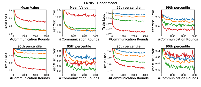
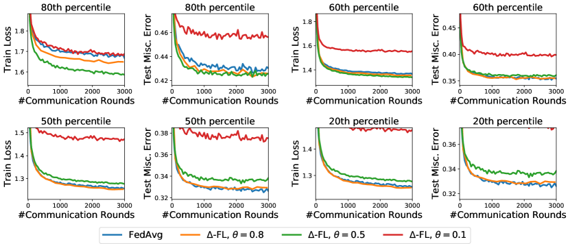
Figure 7: Performance across iterations of EMNIST linear model.

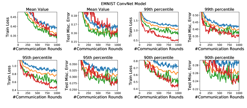
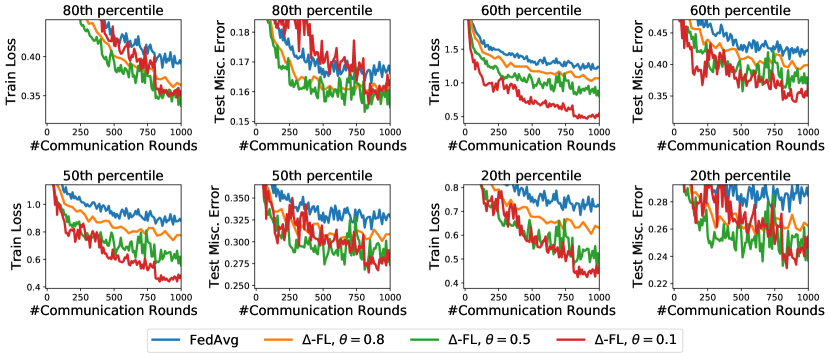
Figure 8: Performance across iterations of EMNIST ConvNet model.

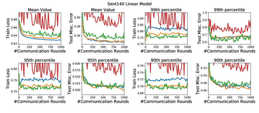
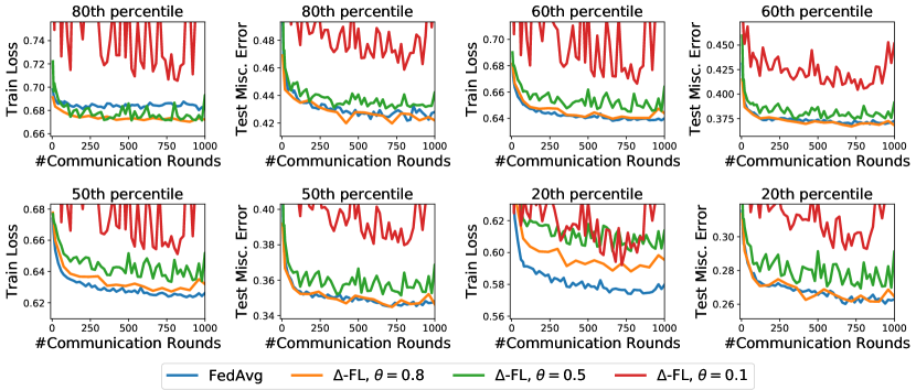
Figure 9: Performance across iterations of Sent140 linear model.

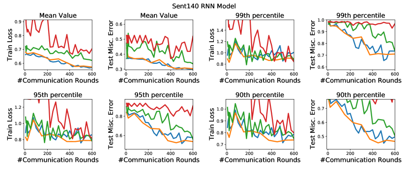
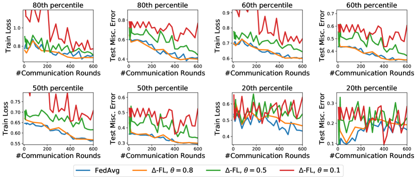
Figure 10: Performance across iterations of Sent140 RNN model.

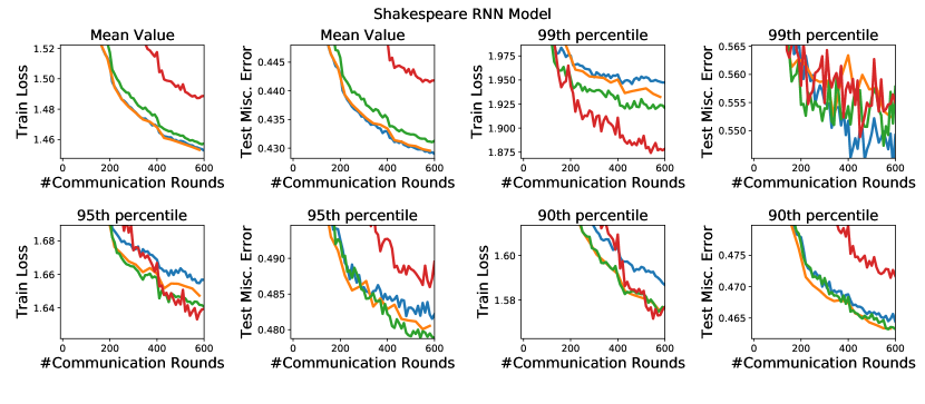
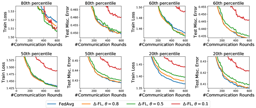
Figure 11: Performance across iterations on the Shakespeare dataset.

Histograms of Loss and Test Misc. Error over Devices.

Here, we plot the histograms of the loss distribution over training devices and the misclassification error distribution over testing devices. We report the losses and errors obtained at the end of the training process. Each metric is averaged per device over 5 runs of the random seed.

Figure 12 shows the histograms for EMNIST, while Figure 13 shows the histograms for Sent140 and Shakespeare.

We note that $\Delta$-FL tends to exhibit thinner upper tails at some values of $\theta$ and often at multiple values of $\theta$. This shows the benefit of using $\Delta$-FL over vanilla FedAvg.

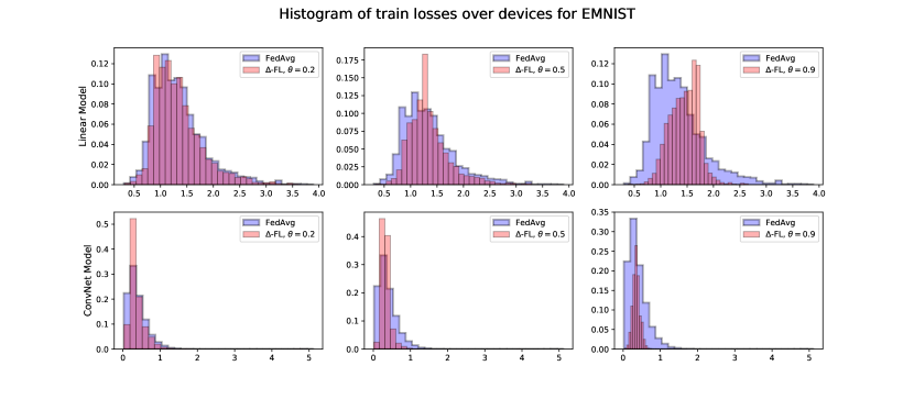
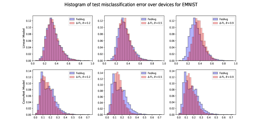
Figure 12: Histogram of loss distribution over training devices and misclassification error distribution over testing devices for EMNIST. The identification of the model (linear or ConvNet) is given on the $y$-axis of the histograms.

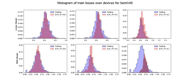
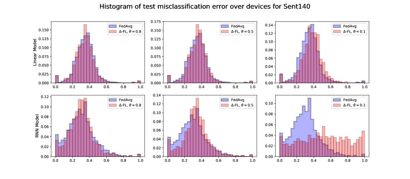
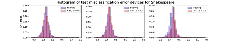
Figure 13: Histogram of loss distribution over training devices and misclassification error distribution over testing devices for Sent140 and Shakespeare. The identification of the model (linear or RNN) is given on the $y$-axis of the histograms.

Performance compared to local data size.

Next, we plot the loss on training devices versus the amount of local data on the device and the misclassification error on the test devices versus the amount of local data on the device. See Figure 14 for EMNIST and Figure 15 for Sent140 and Shakespeare.

Observe, firstly, that $\Delta$-FL reduces the variance of of the loss on the train devices. Secondly, note that amongst test devices with a small number of data points (e.g., $<200$ for EMNIST or $<100$ for Sent140), $\Delta$-FL reduces the variance of the misclassification error. Both effects are more pronounced on the neural network models.

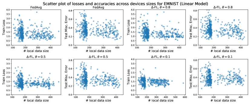
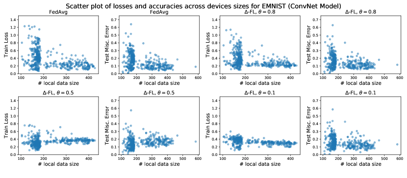
Figure 14: Scatter plot of (a) loss on training device vs. amount of local data, and (b) misclassification error on testing device vs. amount of local data for EMNIST.

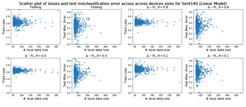
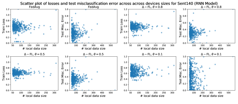
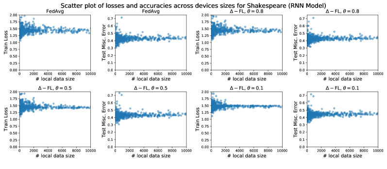
Figure 15: Scatter plot of (a) loss on training device vs. amount of local data, and (b) misclassification error on testing device vs. amount of local data for Sent140 and Shakespeare.

Number of Devices Selected per Communication Rounds.

Next, we plot the number of devices selected per round (after device filtering, if applicable). The shaded area denotes the maximum and minimum over 5 random runs. We see from Figure 16 that device-filtering is stable in the number of devices filtered out.

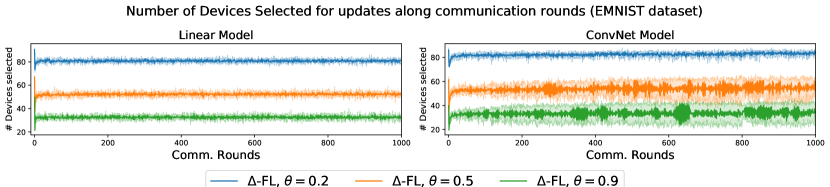
Figure 16: Number of devices selected per round (after device filtering, if applicable) for the EMNIST dataset. The shaded region denotes the maximum and minimum over 5 random runs.

Effect of the Period of Update of $\eta$.

Here, we compare with the experiments to update $\eta$ every $T_{\eta}$ rounds. Equivalently, this amounts to running the $w$-step of the alternation minimization meta-algorithm for $T_{\eta}$ steps. See Figure 17 for EMNIST linear model and Figure 18 for Sent140 linear model. We see that on the Sent140 linear model, the choice of $T_{\eta}$ does not make any difference, while for EMNIST, larger $T_{\eta}$ appears to help. Note that Algorithm 2 corresponds to $T_{\eta}=1$.

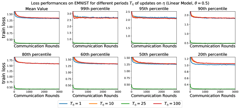
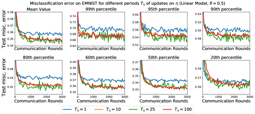
Figure 17: Effect of different choices of $T_{\eta}$ on EMNIST linear model.

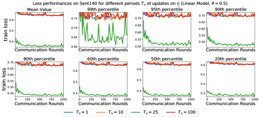
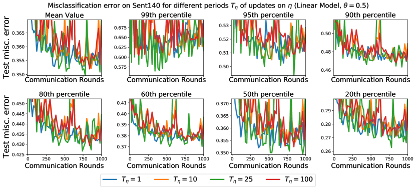
Figure 18: Effect of different choices of $T_{\eta}$ on Sent140 linear model.

Appendix D Properties of Subdifferentials and Smoothing

D.1 Subdifferentials of Non-convex Functions

We briefly recall the standard notions of subgradients for nonsmooth functions. We follow the terminology of standard textbooks [10, 39]. For a function $\varphi\colon\mathbb{R}^{d}\rightarrow\mathbb{R}\cup\{+\infty\}$, we define the regular (or Fréchet) subdifferential of $\varphi$ at $\bar{x}$ as

$$\partial^{R}\varphi(\bar{x})=\{z\in\mathbb{R}^{n}:~{}\varphi(x)\geq\varphi(\bar{x})+{z}^{\top}(x-\bar{x})+o(\|x-\bar{x}\|)\},$$

which corresponds to the set of gradients of smooth functions that are below $\varphi$ and coincide with it at $x$. We then introduce the limiting subdifferential as the set of all limits produced by regular subgradients

$$\partial^{L}\varphi(\bar{x})=\limsup_{x\rightarrow\bar{x},\varphi(x)\rightarrow\varphi(\bar{x})}\partial^{R}\varphi(x).$$

We also consider the (Clarke) subdifferential which can be defined, when $\varphi$ is locally Lipschitz, by the convex hull of the limiting subdifferential:

$$\partial\varphi(\bar{x})=\text{conv}\ \partial^{L}\varphi(\bar{x}).$$

These notions generalize (sub)gradients of both smooth functions and convex functions: for these functions indeed, the three subdifferentials coincide, and they reduce to $\{\nabla\varphi(\bar{x})\}$ when $\varphi$ is smooth and to the standard subdifferential from convex analysis when $\varphi$ is convex.

D.2 Infimal Convolution Smoothing

A convex, non-smooth function $h$ can be smoothed by infimal convolution with a smooth function [32, 3]. We use its dual representation, recalled below.

Definition 15.

For a given convex function $h:\mathbb{R}^{m}\to\mathbb{R}$, a smoothing function $\omega:\operatorname*{dom}h^{*}\to\mathbb{R}$ which is 1-strongly convex with respect to $\|\cdot\|$, and a parameter $\nu>0$, define

$$h_{\nu\omega}(z):=\max_{u\in\operatorname*{dom}h^{*}}\left\{\langle u,z\rangle-h^{*}(u)-\nu\omega(u)\right\}\,.$$

as the smoothing of $h$ by $\nu\omega$.

We now state a classical result showing how the parameter $\nu$ controls both the approximation error and the level of the smoothing. For a proof, see [35, Proposition 39], which is an extension of [3, Theorem 4.1, Lemma 4.2].

Theorem 16.

Consider the setting of Def. 15. The smoothing $h_{\nu\omega}$ is continuously differentiable and its gradient, given by

$$\nabla h_{\nu\omega}(z)=\operatorname*{arg\,max}_{u\in\operatorname*{dom}h^{*}}\left\{\langle u,z\rangle-h^{*}(u)-\nu\omega(u)\right\}$$

is $1/\nu$-Lipschitz with respect to $\|{\cdot}\|^{*}$, the dual norm to $\|\cdot\|$. Moreover, letting $h_{\nu\omega}\equiv h$ for $\nu=0$, the smoothing satisfies, for all $\nu_{1}\geq\nu_{2}\geq 0$,

$$(\nu_{1}-\nu_{2})\inf_{u\in\operatorname*{dom}h^{*}}\omega(u)\leq h_{\nu_{2}\omega}(z)-h_{\nu_{1}\omega}(z)\leq(\nu_{1}-\nu_{2})\sup_{u\in\operatorname*{dom}h^{*}}\omega(u)\,.$$

References

- sim [2020] https://github.com/krishnap25/simplicial-fl, 2020.
- Artzner et al. [1999] P. Artzner, F. Delbaen, J.-M. Eber, and D. Heath. Coherent Measures of Risk. Mathematical finance, 9(3):203–228, 1999.
- Beck and Teboulle [2012] A. Beck and M. Teboulle. Smoothing and First Order Methods: A Unified Framework. SIAM Journal on Optimization, 22(2):557–580, 2012.
- Ben-Tal and Teboulle [2007] A. Ben-Tal and M. Teboulle. An Old-New Concept of Convex Risk Measures: The Optimized Certainty Equivalent. Mathematical Finance, 17(3):449–476, 2007.
- Ben-Tal et al. [2009] A. Ben-Tal, L. El Ghaoui, and A. Nemirovski. Robust Optimization, volume 28. Princeton University Press, 2009.
- Bertsekas and Tsitsiklis [1989] D. P. Bertsekas and J. N. Tsitsiklis. Parallel and Distributed Computation: Numerical Methods, volume 23. Prentice hall Englewood Cliffs, NJ, 1989.
- Bonawitz et al. [2017] K. Bonawitz, V. Ivanov, B. Kreuter, A. Marcedone, H. B. McMahan, S. Patel, D. Ramage, A. Segal, and K. Seth. Practical Secure Aggregation for Privacy-Preserving Machine Learning. In ACM SIGSAC Conference on Computer and Communications Security, pages 1175–1191, 2017.
- Caldas et al. [2018] S. Caldas, P. Wu, T. Li, J. Konečný, H. B. McMahan, V. Smith, and A. Talwalkar. LEAF: A benchmark for federated settings. arXiv Preprint, 2018.
- Cho et al. [2014] K. Cho, B. Van Merriënboer, C. Gulcehre, D. Bahdanau, F. Bougares, H. Schwenk, and Y. Bengio. Learning Phrase Representations using RNN Encoder-Decoder for Statistical Machine Translation. arXiv Preprint, 2014.
- Clarke [1990] F. H. Clarke. Optimization and nonsmooth analysis, volume 5. Siam, 1990.
- Cohen et al. [2017] G. Cohen, S. Afshar, J. Tapson, and A. van Schaik. EMNIST: an extension of MNIST to handwritten letters. arXiv Preprint, 2017.
- Dick et al. [2017] T. Dick, M. Li, V. K. Pillutla, C. White, N. Balcan, and A. Smola. Data Driven Resource Allocation for Distributed Learning. In Artificial Intelligence and Statistics, pages 662–671, 2017.
- Duchi and Namkoong [2019] J. C. Duchi and H. Namkoong. Variance-based Regularization with Convex Objectives. Journal of Machine Learning Research, 20(68):1–55, 2019.
- Eichner et al. [2019] H. Eichner, T. Koren, B. Mcmahan, N. Srebro, and K. Talwar. Semi-Cyclic Stochastic Gradient Descent. In International Conference on Machine Learning, pages 1764–1773, 2019.
- Ferguson [1967] T. S. Ferguson. Mathematical Statistics: A Decision Theoretic Approach. Academic press, 1967.
- Go et al. [2009] A. Go, R. Bhayani, and L. Huang. Twitter Sentiment Classification using Distant Supervision. CS224N Project Report, Stanford, page 2009, 2009.
- He et al. [2018] L. He, A. Bian, and M. Jaggi. COLA: Decentralized Linear Learning. In Advances in Neural Information Processing Systems 31, pages 4541–4551, 2018.
- Hiriart-Urruty and Lemaréchal [1996] J.-B. Hiriart-Urruty and C. Lemaréchal. Convex Analysis and Minimization Algorithms I: Fundamentals. Grundlehren der mathematischen Wissenschaften. Springer Berlin Heidelberg, 1996. ISBN 9783540568506.
- Hochreiter and Schmidhuber [1997] S. Hochreiter and J. Schmidhuber. Long Short-Term Memory. Neural computation, 9(8):1735–1780, 1997.
- Huang et al. [2019] L. Huang, A. L. Shea, H. Qian, A. Masurkar, H. Deng, and D. Liu. Patient Clustering Improves Efficiency of Federated Machine Learning to Predict Mortality and Hospital stay time using Distributed Electronic Medical Records. Journal of Biomedical Informatics, 99:103291, 2019.
- Hunter and Lange [2000] D. R. Hunter and K. Lange. Quantile Regression via an MM Algorithm. Journal of Computational and Graphical Statistics, 9(1):60–77, 2000.
- Jiang et al. [2019] Y. Jiang, J. Konečný, K. Rush, and S. Kannan. Improving Federated Learning Personalization via Model Agnostic Meta Learning. arXiv preprint, 2019.
- Kairouz et al. [2019] P. Kairouz, H. B. McMahan, B. Avent, A. Bellet, M. Bennis, A. N. Bhagoji, K. Bonawitz, Z. Charles, G. Cormode, R. Cummings, R. G. D’Oliveira, S. E. Rouayheb, D. Evans, J. Gardner, Z. Garrett, A. Gasc/’on, B. Ghazi, P. B. Gibbons, M. Gruteser, Z. Harchaoui, C. He, L. He, Z. Huo, B. Hutchinson, J. Hsu, M. Jaggi, T. Javidi, G. Joshi, M. Khodak, J. Konečný, A. Korolova, F. Koushanfar, S. Koyejo, T. Lepoint, Y. Liu, P. Mittal, M. Mohri, R. Nock, A. Özgür, R. Pagh, M. Raykova, H. Qi, D. Ramage, R. Raskar, D. Song, W. Song, S. U. Stich, Z. Sun, A. T. Suresh, F. Tramèr, P. Vepakomma, J. Wang, L. Xiong, Z. Xu, Q. Yang, F. X. Yu, H. Yu, and S. Zhao. Advances and open problems in federated learning. arXiv Preprint, 2019.
- Konečný et al. [2016] J. Konečný, H. B. McMahan, F. X. Yu, P. Richtárik, A. T. Suresh, and D. Bacon. Federated Learning: Strategies for Improving Communication Efficiency. arXiv Preprint, 2016.
- Kuhn et al. [2019] D. Kuhn, P. M. Esfahani, V. A. Nguyen, and S. Shafieezadeh-Abadeh. Wasserstein Distributionally Robust Optimization: Theory and Applications in Machine Learning. In Operations Research & Management Science in the Age of Analytics, pages 130–166. 2019.
- Leblond et al. [2018] R. Leblond, F. Pedregosa, and S. Lacoste-Julien. Improved Asynchronous Parallel Optimization Analysis for Stochastic Incremental Methods. Journal of Machine Learning Research, 19, 2018.
- Lee and Raginsky [2018] J. Lee and M. Raginsky. Minimax statistical learning with Wasserstein distances. In Advances in Neural Information Processing Systems, pages 2687–2696, 2018.
- Li et al. [2020] T. Li, M. Sanjabi, and V. Smith. Fair Resource Allocation in Federated Learning. In International Conference on Learning Representations, 2020.
- Ma et al. [2017] C. Ma, J. Konečný, M. Jaggi, V. Smith, M. I. Jordan, P. Richtárik, and M. Takác. Distributed optimization with arbitrary local solvers. Optimization Methods and Software, 32(4):813–848, 2017.
- McMahan et al. [2017] B. McMahan, E. Moore, D. Ramage, S. Hampson, and B. A. y Arcas. Communication-Efficient Learning of Deep Networks from Decentralized Data. In Artificial Intelligence and Statistics, pages 1273–1282, 2017.
- Mohri et al. [2019] M. Mohri, G. Sivek, and A. T. Suresh. Agnostic Federated Learning. In International Conference on Machine Learning, 2019.
- Nesterov [2005] Y. Nesterov. Smooth minimization of non-smooth functions. Mathematical programming, 103(1):127–152, 2005.
- Nesterov [2013] Y. Nesterov. Introductory Lectures on Convex Optimization Vol. I: Basic course, volume 87. Springer Science & Business Media, 2013.
- Pennington et al. [2014] J. Pennington, R. Socher, and C. D. Manning. GloVe: Global Vectors for Word Representation. In Empirical Methods in Natural Language Processing, pages 1532–1543, 2014.
- Pillutla et al. [2018] K. Pillutla, V. Roulet, S. M. Kakade, and Z. Harchaoui. A Smoother Way to Train Structured Prediction Models. In Advances in Neural Information Processing Systems, pages 4766–4778, 2018. URL https://arxiv.org/pdf/1902.03228.pdf.
- Pillutla et al. [2019] K. Pillutla, S. M. Kakade, and Z. Harchaoui. Robust Aggregation for Federated Learning. arXiv preprint, 2019.
- Rockafellar and Royset [2018] R. T. Rockafellar and J. O. Royset. Superquantile/CVaR Risk Measures: Second-Order Theory. Annals of Operations Research, 262(1):3–28, 2018.
- Rockafellar and Uryasev [2000] R. T. Rockafellar and S. Uryasev. Optimization of Conditional Value-at-Risk. Journal of Risk, 2:21–42, 2000.
- Rockafellar and Wets [2009] R. T. Rockafellar and R. J.-B. Wets. Variational analysis, volume 317. Springer Science & Business Media, 2009.
- Rockafellar et al. [2014] R. T. Rockafellar, J. O. Royset, and S. I. Miranda. Superquantile regression with applications to buffered reliability, uncertainty quantification, and conditional value-at-risk. European Journal of Operational Research, 234(1):140–154, 2014.
- Sahu et al. [2018] A. K. Sahu, T. Li, M. Sanjabi, M. Zaheer, A. Talwalkar, and V. Smith. On the Convergence of Federated Optimization in Heterogeneous Networks. arXiv Preprint, 2018.
- Sattler et al. [2019] F. Sattler, S. Wiedemann, K.-R. Müller, and W. Samek. Robust and Communication-Efficient Federated Learning from Non-IID Data. IEEE Transactions on Neural Networks and Learning Systems, 2019.
- [43] W. Shakespeare. The Complete Works of William Shakespeare. URL https://www.gutenberg.org/ebooks/100.
- Smith et al. [2017] V. Smith, C.-K. Chiang, M. Sanjabi, and A. S. Talwalkar. Federated multi-task learning. In Advances in Neural Information Processing Systems 30, pages 4424–4434, 2017.
- Smith et al. [2018] V. Smith, S. Forte, M. Chenxin, M. Takáč, M. I. Jordan, and M. Jaggi. COCOA: A General Framework for Communication-Efficient Distributed Optimization. Journal of Machine Learning Research, 18:230, 2018.
- Yang et al. [2018] T. Yang, G. Andrew, H. Eichner, H. Sun, W. Li, N. Kong, D. Ramage, and F. Beaufays. Applied Federated Learning: Improving Google Keyboard Query Suggestions. arXiv preprint arXiv:1812.02903, 2018.