Optical Spectroscopy of nearby type1-LINERs
Abstract
We present the highlights from our recent study of 22 local (z 0.025) type-1 LINERs from the Palomar Survey, on the basis of optical long-slit spectroscopic observations taken with TWIN/CAHA, ALFOSC/NOT and HST/STIS. Our goals were threefold: (a) explore the AGN-nature of these LINERs by studying the broad (BLR-originated) H6563 component; (b) derive a reliable interpretation for the multiple narrow components of emission lines by studying their kinematics and ionisation mechanism (via standard BPTs); (c) probe the neutral gas in the nuclei of these LINERs for the first time. Hence, kinematics and fluxes of a set of emission lines, from H4861 to [SII]6716,6731, and the NaD5890,5896 doublet in absorption have been modelled and measured, after the subtraction of the underlying light from the stellar component.
keywords:
galaxies: active, galaxies: kinematics and dynamics, techniques: spectroscopic.P. Shastri, S. B. Tessema S. H. Negu, eds.
1 Introduction
Low ionisation nuclear emission-line regions (LINERs) are a class of low-luminosity AGNs showing strong low-ionisation and faint high-ionisation emission lines ([Heckman (1980), Heckman 1980]). LINERs are interesting objects since they are the most numerous local AGN population bridging the gap between normal and active galaxies ([Ho (2008), Ho 2008]).
Over the past 20 years, the ionising source in LINERs has been studied through a multi-wavelength approach via different tracers ([Ho (2008), Ho 2008]). Nevertheless, a long standing issue is the origin and excitation mechanism of the ionised gas studied via optical emission lines. In addition to the AGN scenario, two more alternatives, such as pAGBs stars and shocks, have been proposed to explain the optical properties of LINERs (e.g. [Singh et al. (2013), Singh et al. 2013]).
In LINERs, outflows are common as suggested by their H nuclear morphology ([Masegosa et al. (2011), Masegosa et al. 2011]). To open a new window to explore the AGN-nature and the excitation mechanism in LINERs, we propose to infer the role of outflows (identified as relatively broad component) in the broadening of emission lines. This broadening effect may limit the spectroscopic classification, as the contribution of outflows may overcome the determination of an eventually faint and broad H component from the BLR.
Ionised gas outflows are observed in starbursts and AGNs via long slit (e.g. [Harrison2012, Harrison et al. 2012]) and integral field spectroscopy (e.g. [Maiolinoet al. (2017), Maiolino et al. 2017]) of emission lines. The neutral gas in outflows have been studied in detail only in starbursts and luminous and ultra-luminous infrared galaxies (U/LIRGs) via the NaD absorption (e.g. [Cazzoli et al. (2016), Cazzoli et al. 2016]).
In [Cazzoli et al. (2018), Cazzoli et al. 2018], hereafter C18, our goals were to investigate the AGN nature of type-1 LINERs and to characterize all the components by studying their kinematics and ionisation mechanisms. We also aimed to probe and study the neutral gas properties.
For type-2 LINERs, see the contribution by L. Hermosa-Muñoz in this volume.
2 Sample, Data and Methods
The sample contains nearby (z 0.025) 22 type-1 LINERs (L1) selected from the Palomar Survey (see [Ho et al. (1997), Ho et al. 1997]). Spectroscopic data were gathered with the TWIN Spectrograph mounted on the 3.5m telescope of the Calar Alto Observatory (CAHA) and with ALFOSC attached to the 2.6m North Optical Telescope (NOT). We also analyzed archival spectra (red bandpass) for 12 LINERs (see [Balmaverde et al. (2014), Balmaverde et al. 2014] for details) obtained with the Space Telescope Imaging Spectrograph (STIS) on board the Hubble Space Telescope (HST). The data analysis is organised in three main steps:
Stellar Subtraction
We applied the penalized PiXel fitting (pPXF; [Cappellari (2017), Cappellari 2017]) and the starlight methods ([Cid Fernandes et al. (2009), Cid Fernandes et al. 2009]) for modeling the stellar continuum. The stellar model is then subtracted to the observed to one obtain a interstellar medium spectrum.
Emission Lines
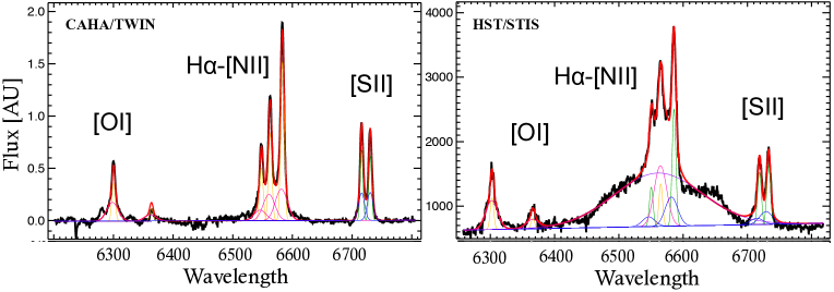
The fit was performed simultaneously for emission lines from [OI]6300,6363 to [SII], with single or multiple Gaussian kinematic components (up two for forbidden lines and narrow H). For the modeling of the H-[NII]6548,6584 blend, we tested three distinct models. Specifically, we considered either [SII] or [OI] (S- and O- models) or both (‘mixed’ M-model) as reference for tying central wavelengths and line widths (see example in Fig. 1). The latter model takes into account possible stratification density in the narrow line region. Then, a broad H component is added if needed to reduce significantly the residual. Finally, the best fitting (i.e. model, components, velocity shift and line widths) has been constraint to be the same for [OIII]4959,5007 and H lines. Intensity ratios for [NII], [OI] and [OIII] lines were imposed following [Osterbrock et al. (2006), Osterbrock 2006].
Absorption Lines
The NaD absorption doublet (8 detections) was modelled with one (i.e. two Gaussian profiles) or two components as in [Cazzoli et al. (2014), Cazzoli et al. 2014]. The ratio of the equivalent widths of the two lines was allowed to vary from 1 to 2 (i.e. optically thick/thin limits, [Spitzer (1978), Spitzer 1978]).
3 Main Results
NGC 4203 represents an extreme case as three line components are not sufficient to reproduce well the H profile, therefore, we excluded this L1 from the analysis.
For ground-based data, the S- and O- models reproduce well the line profiles in six of the cases each, while a larger fraction of cases (i.e. 9/21) require M-models for a satisfactory fit. Of the four possible combinations of the three components, as single narrow Gaussian per forbidden line is adequate in 6 out of 21 cases. A broad H component is required in the remaining four cases. In most cases (15/21), two Gaussians per forbidden line are required for a satisfactory modelling. Among these 15 cases, only in three cases a broad H component is required to reproduce well the observed profiles.
Velocities of the narrow components are close to rest frame varying within 110 km s-1. The average velocity dispersion value for the narrow components is = 157 km s-1. For the second components the velocity range is large, from -350 km s-1 to 100 km s-1. The velocity dispersion varies between 150 and 800 km s-1 being generally broader (on average = 429 km s-1) than for narrow components. A broad H component is required only in 7 out of the 21 LINERs, with FWHMs from 1277 km s-1 to 3158 km s-1.
For none of the 11 HST/STIS spectra, the adopted best fit is obtained using the O-model, finding a slightly large prevalence of best fits with M-models. In four cases, one Gaussian per forbidden line and narrow H is adequate. In the remaining cases, two Gaussians are required for a good fit.
Narrow components have velocities between -100 and 200 km s-1; the velocity dispersions vary between 120 and 270 km s-1 (176 km s-1, on average). Similarly, the velocities of second component range from -200 to 150 km s-1. These second components are however broader, with velocity dispersion values between 300 and 750 km s-1 (433 km s-1, on average). The broad component in is ubiquitous. The FWHM of the broad H components in HST spectra range from 2152 km s-1 to 7359 km s-1 (3270 km s-1, on average).
For the NaD absorption, in 7 out of 8 targets, a single kinematic component gives a good fit. Velocities of the neutral gas narrow components vary between -165 and 165 km s-1; velocity dispersions values are in the range 104-335 km s-1 (220 km s-1, on average).
4 Discussion
Probing the BLR in L1
The analysis of Palomar spectra by [Ho et al. (1997), Ho et al. (1997)] indicated that all the LINERs in our selected sample show a broad H component resulting in their classification as L1. Nevertheless, for ground-based data our detection rate for the broad component is only 33 , questioning the classification as L1 by [Ho et al. (1997), Ho et al. (1997)]. For space-based data the broad component is ubiquitous in agreement with [Balmaverde et al. (2014), Balmaverde et al. 2014]. By comparing our strategy and measurements with those by previous works (Sect. 5.1 in C18), we conclude that the detectability of the BLR-component is sensitive to the starlight decontamination and the choice of the template for the H-[NII] blend. Moreover, a single Gaussian fit for the forbidden lines is an oversimplification in many cases.
Kinematic classification of the components
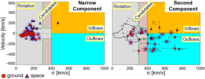
The distribution of the velocity for narrow and second components as a function of their velocity dispersion is presented in Fig. 3. We identified four areas corresponding to different kinematical explanations: rotation, candidate for non-rotational motions and non-rotational-motions (with broad blue/redshifted lines produced by outflows/inflows). For both ground- and space-based data, the kinematics of the narrow component can be explained with rotation in all cases (Fig. 2 left) whereas that of the second components encompass all possibilities (Fig. 2, right). From our ground-based data, we identified 6 out of 15 (40 ) cases that may be interpreted as outflows. Outflow-components have velocities varying from -15 km s-1 to -340 km s-1, and velocity dispersions in the range of 450-770 km s-1 (on average, 575 km s-1). We did not interpreted as outflows any case in HST/STIS data. These results partially disagree with studies of the H morphology in LINERs which indicate that outflows are frequent in LINERs. A possible explanation is that the extended nature of outflows is not fully captured by the HST/STIS spectra.
Ionisation mechanisms from standard ‘BPT (Baldwin, Phillips & Terlevich)-diagrams’
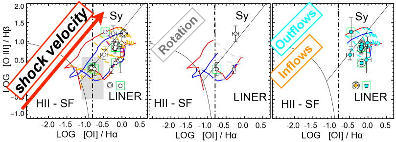
The line ratios for the narrow component are generally consistent with those observed in AGNs (either Seyfert or LINERs), excluding the star-formation or pAGBs as the dominant ionization mechanism (see Fig. 9 in C18). For the second component, we reproduced the observed line ratios with the shock-models by [Groves et al. (2004), Groves et al. 2004]. We combined the data points and models for the [O I]/H BPT diagram ([Baldwin et al. (1981), Baldwin et al. 1981]), the most reliable for studying shocks ([Allenet al. (2008), Allen et al. 2008]) shown in Fig. 3, with the kinematical classification shown in Fig. 3.
Models at low velocities ( 300 km s-1) indicate the presence of mild-shocks associated to perturbations of rotation (Fig. 3 center). At higher velocities ( 400 km s-1) shocks are produced by non-rotational motions (Fig. 3 right).
A lack of neutral outflows?
According to the adopted kinematic classification all the neutral gas kinematic components (except one) could be interpreted as rotation. The possible explanation of the lack of neutral gas non-rotational motions, such as outflows, is twofold. First, the neutral component in outflows is possibly less significant in AGNs than in starbursts galaxies and U/LIRGs. Secondly, such a null detection rate might be a consequence of the conservative limits we assumed, as ionised and neutral gas correspond to different phases of the outflows, and hence these may have a different kinematics (e.g. [Cazzoli et al. (2016), Cazzoli et al. 2016]).
5 Conclusions
The AGN nature of L1. The detection of the BLR-component is sensitive to the starlight subtraction, the template for the H-[NII] blend and the assumption of a single Gaussian fit (often an oversimplification); NLR stratification might be often present in L1.
Kinematics of emission lines and their classification. The kinematics of the narrow component can be explained with rotation in all cases whereas that of the second components encompass all possibilities. From our ground-based data, the detection rate of outflows is 40 . We did not interpreted as outflows any case in HST/STIS data.
Ionisation mechanisms. Our results favor the AGN photoionisation as the dominant mechanism of ionisation for the narrow component. Shocks models (at the observed velocities) are able to reproduce the observed line ratios of the second component.
Neutral gas in L1. The neutral gas is found to be in rotation. Neutral gas outflows are possibly less significant in AGNs or the limits we assumed are too conservative.
Acknowledgements
We thank the financial support by the Spanish MCIU and MEC, grants SEV-2017-0709 and AYA 2016-76682-C3. SC thanks the IAU for the travel grant.
References
- [Allenet al. (2008)] Allen M. G., Groves B. A., Dopita M. A. et al. 2008, ApJS, 178, 20
- [Balmaverde et al. (2014)] Balmaverde & Capetti 2014, A&A, 563, A119
- [Baldwin et al. (1981)] Baldwin, Phillips & Terlevich 1981, PASP, 93, 5
- [Binette et al. (1994)] Binette L., Magris C. G., Stasinska G., Bruzual A. G 1994, A&A, 292, 13
- [Cazzoli et al. (2018)] Cazzoli S., Marquez I., Masegosa J. et al. 2018, MNRAS, 480, 1106
- [Cazzoli et al. (2016)] Cazzoli S., Arribas S., Maiolino R. & Colina L. 2016, A&A, 590, A125
- [Cazzoli et al. (2014)] Cazzoli S., Arribas S., Colina L., et al. 2014, A&A, 569, A14
- [Cappellari (2017)] Cappellari M. 2017, MNRAS, 466, 798
- [Cid Fernandes et al. (2009)] Cid Fernandes R., Stasinska G., Schlickmann M. et al. 2009, Rev. Mex. Astron. Astrofis., 35, 127
- [Filippenko Terlevich] Filippenko A. V. Terlevich R. 1992, ApJ, 397, L79
- [Groves et al. (2004)] Groves B. A., Dopita M. A. Sutherland R. S. 2004, ApJS, 153, 75
- [Heckman (1980)] Heckman 1980, A&A, 87, 152
- [Ho et al. (1997)] Ho L. C., Filippenko A. V., Sargent W. L. W. 1997, ApJS, 112, 315
- [Ho (2008)] Ho L. C. 2008, ARA&A, 46, 475
- [Kewley et al. (2006)] Kewley L. J., Groves B., Kauffmann G. Heckman T. 2006, MNRAS, 372, 961
- [Kauffmann et al. (2003)] Kauffmann G., Heckman, T., Tremonti, C. et al. 2003, MNRAS, 346, 1055
- [Maiolinoet al. (2017)] Maiolino R., Russel H., Fabian A. et al. 2017, Nature, 544, 202
- [Masegosa et al. (2011)] Masegosa J., Marquez I., Ramirez A. et al. 2011, A&A, 527, A23
- [Osterbrock et al. (2006)] Osterbrock D. E., et al. 2006, Astrophysics of Gaseous Nebulae and Active Galactic Nuclei
- [Singh et al. (2013)] R. Singh G., van de Ven K., Jahnke, M. et al. 2013, A&A, 558, A43
- [Spitzer (1978)] Spitzer L. 1978, Physical Processes in the Interstellar Medium. Wiley-Interscience, New York