Golrezaei et al.

Dynamic Incentive-Aware Learning: Robust Pricing in Contextual Auctions

Dynamic Incentive-aware Learning: Robust Pricing in Contextual Auctions

Negin Golrezaei Sloan School of Management, Massachusetts Institute of Technology, Cambridge, MA, golrezae@mit.edu Adel Javanmard Data Sciences and Operations Department, University of Southern California, Los Angeles, CA, ajavanma@usc.edu Vahab Mirrokni Google Research, New York, NY, mirrokni@google.com

Motivated by pricing in ad exchange markets, we consider the problem of robust learning of reserve prices against strategic buyers in repeated contextual second-price auctions. Buyers’ valuations for an item depend on the context that describes the item. However, the seller is not aware of the relationship between the context and buyers’ valuations, i.e., buyers’ preferences. The seller’s goal is to design a learning policy to set reserve prices via observing the past sales data, and her objective is to minimize her regret for revenue, where the regret is computed against a clairvoyant policy that knows buyers’ heterogeneous preferences. Given the seller’s goal, utility-maximizing buyers have the incentive to bid untruthfully in order to manipulate the seller’s learning policy. We propose learning policies that are robust to such strategic behavior. These policies use the outcomes of the auctions, rather than the submitted bids, to estimate the preferences while controlling the long-term effect of the outcome of each auction on the future reserve prices. When the market noise distribution is known to the seller, we propose a policy called Contextual Robust Pricing (CORP) that achieves a T-period regret of $O(d\log(Td)\log(T))$, where $d$ is the dimension of the contextual information. When the market noise distribution is unknown to the seller, we propose two policies whose regrets are sublinear in $T$. pricing, robust learning, strategic buyers repeated second-price auctions, online advertising

1 Introduction

In many online marketplaces, both sides of the market have access to rich dynamic contextual information about the products that are being sold over time. On the buying side, such information can influence the willingness-to-pay of the buyers for the products, potentially in a heterogeneous way. On the selling side, the information can help the seller differentiate the products and set contextual and possibly personalized prices. To do so, the seller needs to learn the impact of this information on buyers’ willingness-to-pay. Such contextual learning can be challenging for the seller when there are repeated interactions between the buying and the selling sides. With repeated interactions, the utility-maximizing buyers may have the incentive to act strategically and trick the learning policy of the seller into lowering their prices. Motivated by this, our key research question is as follows: How can the seller dynamically optimize (personalized) prices in a robust manner, taking into account the strategic behavior of the buyers?

One of the online marketplaces that faces this problem is the online advertising market. In this market, a prevalent approach to sell ads is via running real-time second-price auctions in which advertisers can use an abundance of detailed contextual information before deciding what to bid. In this practice, advertisers can target Internet users based on their (heterogeneous) preferences and targeting criteria. Targeting can create a thin and uncompetitive market in which few advertisers show interest in each auction. In such a thin market, it is crucial for the ad exchanges to effectively optimize the reserve prices in order to boost their revenue. However, learning the optimal reserve prices is rather difficult due to frequent interactions between advertisers and ad exchanges.

Inspired by this environment, we study a model in which a seller runs repeated (lazy) second-price auctions with reserve over time. In the lazy auction, an item is being sold to the buyer with the highest submitted bid as long his bid exceeds his reserve. The valuation (willingness-to-pay) of each buyer for the item in period $t$, which is his private information, depends on an observable $d$-dimensional contextual information in that period and his preference vector. We focus on an important special case of this contextual-based valuation model in which the buyer’s value is a linear function of his preference vector and contextual information, plus some random noise term, where the noise models the impact of contexts that are not measured/observed by the seller. The preference vector, which is unknown to the seller and fixed throughout the time horizon, varies across buyers. Thus, the preference vectors capture heterogeneity in buyers’ valuation.

The seller’s goal is to design a policy that dynamically learns/optimizes personalized reserve prices. The buyers are fully aware of the learning policy used by the seller and act strategically in order to maximize their (time-discounted) cumulative utility. Dealing with such a strategic population of buyers, the seller aims at extracting as much revenue as the clairvoyant policy that is cognizant of the preference vectors a priori. These vectors determine the relationship between the valuation of the buyers and contextual information. Put differently, the seller would like to minimize her regret where the regret is defined as the difference between the seller’s revenue and that under the clairvoyant policy. Note that the clairvoyant policy provides a strong benchmark because the policy posts the optimal personalized reserve prices based on the observed contexts.

As stated earlier, the main hurdles in designing a low-regret learning policy in this setting are the frequent interactions between the seller and the buyers. Due to such interactions, the strategic buyers might have the incentive to bid untruthfully. This way, they may sacrifice their short-term utility in order to deceive the seller, to post them lower future reserve prices. Thus, while a single shot second-price auction is a truthful mechanism, repeated second-price auctions in which the seller aims at dynamically learning optimal reserve prices of strategic and utility-maximizing buyers may not be truthful. The untruthful bidding behavior of the buyers makes it hard for the seller to learn the optimal reserve prices, and this, in turn, can lead to her revenue loss. This highlights the necessity to design a robust learning policy that reduces buyers’ incentive to follow untruthful strategy. Beside this hurdle, the availability of the dynamic contextual information requires the seller to change the reserve prices dynamically over time, based on the contextual information. To do so, the seller needs to learn how buyers react to such information and based on the reactions, posts (dynamic) personalized reserve prices. The need to have a personalized reserve price is caused by heterogeneity in buyers’ preferences.

We consider setting where the seller (firm) is more patient than the buyer. We formalize it by considering time-discounted utility for the buyers. This is motivated by various applications. For example, in online advertisement markets, the advertisers (buyers) who retarget Internet users prefer showing their ads to the users who visited their website sooner rather than later.

In this paper, we propose three learning policies. The first policy, which we call Contextual Robust Pricing (CORP), is tailored to a setting where the distribution of the noise term in buyers’ valuation is known to the seller. We will refer to this noise as market or valuation noise. By studying this setting, we can characterize the seller’s revenue loss due to her lack of knowledge about the buyers’ (heterogeneous) response to contextual information. The second policy, that we call CORP-II, is a variant of the first policy. This policy lends itself to a setting where the unknown market noise distribution is fixed throughout the time horizon and belongs to a location–scale family. The third policy, which is called Stable CORP (SCORP), is designed to the setting where the market noise distribution varies over time and as a result, the seller does not have the intention of learning the market noise distribution. She instead would like to design a learning policy that is robust to the uncertainty in the noise distribution.

In the remaining part of the introduction, we briefly discuss the salient characteristics of each policy separately and defer the formal description to Sections 4 and 5.

• CORP Policy: When the market noise distribution is known to the seller, under a log-concavity assumption on the noise distribution, our CORP policy gets the cumulative T-period regret of order $O\left(Nd\left(\log(Td)\log(T)+\frac{\log^{2}(T)}{\log^{2}(1/\gamma)}\right)\right)$, where the regret is computed against the clairvoyant policy that knows the preference vectors as well as the market noise distribution. Here, $N$ is the number of buyers, $\gamma$ is the buyers’ discount factor, and $O\left(Nd\frac{\log^{2}(T)}{\log^{2}(1/\gamma)}\right)$ is the extra regret due to the strategic behavior of the buyers. The policy works in an episodic manner where the length of episodes doubles each time. Some of the periods in each episode are randomly assigned to exploration, and the rest of the periods are dedicated to exploitation. At the beginning of each episode, CORP updates its estimates of the preference vectors by running a maximum Likelihood estimator using only the auction outcomes from the previous episode and then adheres to those estimates throughout the episode. During the exploitation periods, CORP sets the reserves based on its estimates of the preference vectors and its knowledge of the noise distribution. As time progresses, the policy becomes more confident about its estimates and consequently uses those estimate over a longer episode.

  We now highlight two important aspects of CORP. As explained earlier, the CORP policy has an episodic structure and updates its estimate of preference vectors only at the beginning of each episode. Such design makes the policy robust by restricting the future effect of the submitted bids. Specifically, bids in an episode are not used in choosing the reserve prices until the beginning of the next episode. Therefore, there is always a delay until a buyer observes the effect of a bid on reserves. Then, considering the fact that buyers are impatient and discount the future, they are more incentivized to bid truthfully.

  There is another important aspect of the policy that ensures its robustness: its estimation method. Rather than using the submitted bids to estimate the preference vectors, the policy simply uses the outcome of the auctions. Because of this feature of the policy, bidding untruthfully does not always result in lower reserve prices; instead, it can impact the future reserve prices of a buyer when it leads to changing the outcome of an auction, i.e., when a buyer loses an auction due to underbidding or a buyer wins an auction due to overbidding. As it becomes more clear later, the CORP-II and SCORP policies are also designed in a way to enjoy the aforementioned robustness properties.

• CORP-II Policy: We design this policy for the setting where market noise distribution, which is fixed throughout time horizon, is unknown and belongs to a location–scale family. This policy obtains a regret in the order of $O\left(Nd\log(Td)\sqrt{T}+N^{2}d\Big{(}1+\frac{1}{\log^{2}(1/\gamma)}\Big{)}\log^{3}(T)\right)$ against a clairvoyant policy that knows the preference vectors and market noise distribution. Similar to the CORP policy, CORP-II estimates the preference vectors and parameters of the market noise distribution using a maximum Likelihood estimator. It also enjoys an episodic structure. However, due to uncertainty in the market noise distribution, the length of the episodes grows at a slower rate, compared with that in CORP.

• SCORP Policy: Our SCORP policy is designed for a setting where the time-varying market noise distribution is unknown to the seller and belongs to an ambiguity set. Then, under the log-concavity assumption on the noise distribution, our policy that knows the ambiguity set, obtains the T-period regret of order $O\left(N\sqrt{d\log(Td)}\;T^{2/3}+{{\color[rgb]{0,0,0}{\frac{N}{\log(1/\gamma)}\log(T)\;T^{1/3}}}}\right)$. Here, the regret is computed against a benchmark called robust; see Definition 5.1. The robust benchmark bears some resemblance to the benchmark used in the regret analysis of CORP; it knows the true preference vectors and the ambiguity set and based on this knowledge chooses the reserve prices that work well against the worst distribution in the ambiguity set. In contrast to the benchmark used in CORP-II, the benchmark here does not intend to learn the noise distribution, as the distribution of the noise can be time-varying. It instead posts “robust” reserve prices.

  The increase in the regret, compared to CORP-II, is due to the fact that the noise distribution is time-varying and as a result, the seller cannot hope to learn it. Because of this, the policy spends more time on exploration compared to CORP-II, which leads to its higher regret. SCORP uses the same episodic structure as CORP-II but dedicates the beginning portion of each episode to pure exploration. Concretely, in episode $k$, with length $\ell_{k}$, pure exploration phase consists of $\lceil\ell_{k}^{2/3}\rceil$ periods. Spending more time on exploration is not the sole difference between CORP-II and SCORP. Given that the noise distribution is time-varying, SCORP uses a least-square estimator to update the estimates of preference vectors, while CORP-II employs the maximum Likelihood estimator, taking advantage of the fact the market noise distribution is fixed and belongs to a location–scale family.

The rest of the paper is organized in the following manner. In Section 2, we review the literature related to our work. Section 3 formally defines our model. We present the CORP in Section 4 and present CORP-II and SCORP policies in Section 5. Finally, we conclude in Section 6.

This paper has an electronic companion. Appendix 7 reviews lower bounds on regret in different pricing settings. In Appendix 8, we provide a discussion on (i) extending our policies to a setting with some non-linear valuation models, and (ii) learning how to price when data is perishable. Appendices 9, 10, and 11 provide the proof of the regret bound of CORP, CORP-II, and SCORP, respectively.

2 Related Work

In this section, we briefly discuss the literature related to our work.

Dynamic Pricing with Learning: Our work is related to the growing body of research on dynamic pricing with learning; see (den Boer 2015) for a survey. (Rothschild 1974, Araman and Caldentey 2009, Farias and Van Roy 2010, Harrison et al. 2012, Cesa-Bianchi et al. 2015, Ferreira et al. 2016, Cheung et al. 2017) studied dynamic pricing with demand uncertainty in the non-contextual and Bayesian settings. In contrast, (Broder and Rusmevichientong 2012, den Boer and Zwart 2013, Besbes and Zeevi 2009) studied this type of problems in the frequentist settings. In these settings, the parameters of the model, which are unknown (but fixed), are estimated using the maximum Likelihood (ML) method or other estimation techniques. We note that there are two important aspects that distinguish our work from this line of literature: the presence of the contextual information and strategic behavior of the buyers. In the following, we elaborate on these aspects by reviewing the related work.

Contextual Dynamic Pricing with Learning in Non-strategic Environment: Recently, several works considered the problem of dynamic pricing in a non-strategic setting when the unknown demand function depends on the customers’ characteristics (aka contextual information). In such settings, customers are not strategic in a sense that they do not consider the impact of their current actions on the future prices they will see. Chen et al. (2015) studied this problem when the demand function follows the logit model and proposed an ML-based learning algorithm. Leme and Schneider (2018), Cohen et al. (2016), and Lobel et al. (2016) proposed a learning algorithm based on the binary search method when the demand function is linear and deterministic. In their models, buyers have homogenous preference vectors and are non-strategic. Hence, the problem reduces to a single buyer setting, where the buyer acts myopically, i.e., the buyer does not consider the impact of the current actions on the future prices. In our setting, however, the seller interacts with a heterogeneous set of buyers in repeated second-price auctions, rather than the posted-price mechanism. Thus, the seller should estimate a preference vector per buyer and use these estimates to set personalized contextual-based reserve prices. There is also a new line of literature that studied dynamic pricing with demand learning when the contextual information is high dimensional (but sparse); see Javanmard and Nazerzadeh (2019), Ban and Keskin (2017). Similar problems have been investigated in Bastani and Bayati (2015), Javanmard (2017).

As mentioned earlier, in our setting, the seller repeatedly interacts with a small number of strategic and heterogeneous buyers. We note that Edelman and Ostrovsky (2007) presented empirical evidence that showed buyers in online advertising markets act strategically. There is also a large body of literature that studied dynamic pricing in a setting where buyers are strategic and the demand function is known a priori; see, for example, Borgs et al. (2014), Besbes and Lobel (2015), Golrezaei et al. (2017b). This literature highlights the importance of considering the strategic behavior of buyers in updating prices over time.

Pricing with Strategic Buyers and Demand Learning: Amin et al. (2013), Medina and Mohri (2014), and Kanoria and Nazerzadeh (2017) examined the problem of dynamic pricing with strategic buyers in a non-contextual environment. In Amin et al. (2013) and Medina and Mohri (2014), the seller repeatedly interacts with a single strategic buyer via a posted-price mechanism. Similar to our setting, the seller is more patient than the buyer in a sense that the buyer discounts his future utility. Amin et al. (2013) showed that no learning algorithm can obtain a sub-linear regret when the buyer is as patient as the seller. In addition, via designing learning policies, they demonstrated that the seller can get a sub-linear regret bound when the buyer is less patient.

Kanoria and Nazerzadeh (2017) studied dynamic pricing when a group of strategic buyers competes with each other in repeated non-contextual second-price auctions. A main difference with our setting is that in their model, buyers are as patient as the firm and hence there is no time-discount factor for buyers’ utilities. They designed a near-optimal elegant pricing policy in which the reserve price of each buyer is computed using the submitted bids of other buyers. Specifically, for any $\epsilon>0$, their policy can be designed to achieve $(1-\epsilon)$ of the expected revenue obtained under the static Myerson optimal auction for the valuation distribution. Note that this corresponds to a linear regret bound in our terms. Indeed in the setting that buyers do not discount their future utilities and buyers are utility-maximizer, it is impossible to get a sub-linear regret (Amin et al. 2013). Further, in (Kanoria and Nazerzadeh 2017) it is assumed that products to be sold are ex-ante identical, and that buyers are homogenous and their valuations are all drawn from a single distribution, which is unknown to the seller.

With respect to the homogeneity assumption, we point out that there exists empirical evidence that buyers are indeed heterogeneous (Guimaraes and Sheedy 2011, Johnson and Myatt 2003, Golrezaei et al. 2017a). It is not surprising that the heterogeneity in the markets makes the design of selling mechanisms more difficult. In addition, such difficulties get more severe when the seller needs to design dynamic selling mechanisms for a group of strategic buyers that compete with each other repeatedly.

Recently, Mahdian et al. (2017) studied a similar problem in a static non-contextual setting where the seller has access to $m$ (strategic) data points and using these data points, she would like to design a mechanism that can incentivize the buyers to be truthful in the first place. They show that when the market power of each buyer is negligible, designing such a mechanism is feasible. To achieve this result, they apply the technique of differential privacy (McSherry and Talwar 2007).

Closer to the spirit of this paper, Amin et al. (2014) studies the problem of pricing inventory in a repeated posted-price auction. The authors propose a pricing algorithm whose regret is in the order of $O(\sqrt{\log T}\,T^{2/3})$ in a contextual setting, against a strategic buyer. We point out that our regret result improves upon Amin et al. (2014) in the following directions:

• We allow for market noise in our model, whereas Amin et al. (2014) considers noiseless setting which posits that buyer’s valuation is given as a linear function of features. Due to this difference, their algorithm and regret bound obtained for noiseless setting in Amin et al. (2014) cannot be applied to our noisy setting and vice versa. Nonetheless, by adding the noise component, we make the model richer. When the noise distribution is known, our CORP policy obtains a T-period regret of $O(d\log(Td)\log(T))$. In addition, when the noise distribution is unknown, our SCORP policy, which is doubly robust against strategic buyers and the uncertainty in the noise distribution, obtains a T-period regret of $O(d\sqrt{\log(Td)}\;T^{2/3})$.

• We consider a market of strategic buyers who participate in a second-price auction at each round, while Amin et al. (2014), motivated by targeting in online advertising, considers a single buyer case. Note that in case of a single buyer, there is no notion of bid, as the buyer only needs to decide if he is willing to purchase the item at the posted price. By contrast, in a market of buyers, each submitted bid of a buyer can potentially affect the utility of that buyer (instant and long-term utility), other buyers’ utilities and the seller’s revenue. We note that Section 5 in Amin et al. (2014) considers an extension to the multiple buyers case but assumes that the highest valuation in each period $t$ can be written as $\langle x_{t},\beta\rangle$ for a fixed parameter vector $\beta$, and product feature (context) $x_{t}$, which we find to be a strong assumption.

Behavior-based Pricing: Our work is also related to the literature on behavior-based pricing where the seller uses the past behavior of the buyers to update the prices (Hart and Tirole 1988, Schmidt 1993, Fudenberg and Villas-Boas 2006, Acquisti and Varian 2005, Esteves et al. 2009, Bikhchandani and McCardle 2012). In this literature, it is mostly assumed that the buyer’s valuation, which is drawn from a publicly known distribution, is fixed throughout the time horizon. Thus, the seller does not need to learn the valuation distribution; instead, the seller aims at learning the realized valuation of the buyer. Note that considering a static valuation for a buyer in the online advertising market is not reasonable, as in this market, buyer’s valuation can depend on the rich contextual information, which varies over time. We also note that in the behavior-based pricing literature, the seller and buyer usually get engaged in repeated games, where each of the player responds to other player’s strategy to form a perfect Bayesian Nash equilibrium.

3 Model

Before we describe the model, we adopt some notation that will be used throughout the paper. For an integer $a$, we write $[a]=\{1,2,\dotsc,a\}$. In addition, for a vector $v\in{\mathbb{R}}^{d}$, we denote its $j^{\text{th}}$ coordinates by $v_{j}$, for $j\in[d]$, and indicate its $\ell_{2}$ norm by $\|v\|$. For two vectors $v,u\in{\mathbb{R}}^{d}$, $\langle u,v\rangle=\sum_{j=1}^{d}u_{j}v_{j}$ represents their inner product. Finally, ${\mathbb{I}}(\cdot)$ denotes the indicator function: ${\mathbb{I}}(A)=1$ when event $A$ happens, and is zero otherwise.

We consider a firm who runs repeated second-price auctions with personalized reserve over a finite time horizon with length $T$. In each period $t\geq 1$, the firm would like to sell an item to one of $N$ buyers. The item in period $t$ is represented by an observable feature (context) vector denoted by $x_{t}\in{\mathbb{R}}^{d}$. We assume that the features are drawn independently from a fixed distribution ${\cal D}$, with a bounded support ${\cal{X}}\subseteq{\mathbb{R}}^{d}$. Note that the length of the time horizon $T$ and distribution ${\cal D}$ are unknown to the firm. For the sake of normalization and without loss of generality, we assume that $\|x_{t}\|\leq 1$, and hence take ${\cal{X}}=\{x\in{\mathbb{R}}^{d}:\,\|x\|\leq 1\}$. We let $\Sigma_{x}={\mathbb{E}}[x_{t}x_{t}^{\sf T}]$ be the second moment matrix of distribution ${\cal D}$, and assume that $\Sigma_{x}$ is a positive definite matrix, where $\Sigma_{x}$ is unknown to the firm.

For buyers’ valuations, we consider a feature-based model that captures heterogeneity among the buyers. In the following, we discuss the specifics of the valuation model. Valuation of buyer $i\in[N]$ for an item in period $t\geq 1$ depends on the feature vector $x_{t}$ and period $t$ and is denoted by $v_{it}(x_{t})$. We assume that $v_{it}(x_{t})$ is a linear function of a preference vector $\beta_{i}$ and the feature vector $x_{t}$. (We relax this assumption in Appendix 8.) That is,

$$v_{it}(x_{t})=\langle x_{t},\beta_{i}\rangle+z_{it}~{}~{}~{}~{}~{}i\in[N],~{}t\geq 1\,.$$ (1)

Whenever it is clear from the context, we may remove the dependency of valuation $v_{it}(x_{t})$ on the feature vector $x_{t}$ and denote it by $v_{it}$. Here, $\beta_{i}\in\mathbb{R}^{d}$ represents the buyer $i$’s preference vector, and for the sake of normalization, we assume that $\|\beta_{i}\|\leq B_{p}$, $i\in[N]$, where $B_{p}$ is a constant. The terms $z_{it}$’s, $i\in[N]$, $t\geq 1$, which are independent of the feature vector $x_{t}$, are idiosyncratic shocks and are referred to as noise. The noise terms are drawn independently and identically from a mean zero distribution $F:[-B_{n},B_{n}]\rightarrow[0,1]$ with continuous density $f:[-B_{n},B_{n}]\rightarrow\mathbb{R}^{+}$, where $B_{n}$ is a constant. We assume that the firm knows the distribution of the noise $F$. We relax this assumption later in Section 5. Note that the valuation of buyer $i$, $v_{it}$, is not known to the firm, as the preference vector $\beta_{i}$ and realization of the noise $z_{it}$ are not observable to her. In addition, by our normalization, $v_{it}(x_{t})\leq B$, with $B=B_{p}+B_{n}$.

We make the following assumption on distribution of the noise $F$.

[Log-concavity] $F(z)$ and $1-F(z)$ are log-concave in $z\in[-B_{n},B_{n}]$.

Assumption 3, which is prevalent in the economics literature (Bagnoli and Bergstrom 2005), holds by several common probability distributions including uniform, and (truncated) Laplace, exponential, and logistic distributions. A few remarks are in order regarding Assumption 1. If distribution $F$ is log-concave and its density $f$ is symmetric, i.e., $f(z)=f(-z)$, then $1-F(z)=F(-z)$ is also log-concave. Moreover, if density $f$ is log-concave, the cumulative distribution function $F$ and the reliability function $1-F$ are also log-concave (Bagnoli and Bergstrom 2005). This implies that Assumption 3 is satisfied when the density $f$ is log-concave. We also point out that if a density has a monotone hazard rate (MHR), i.e., $\dfrac{f(z)}{1-F(z)}$ is increasing in $z$, then $1-F(z)$ is log-concave. This point, in turn, shows that all MHR and symmetric densities satisfy Assumption 3.

We next describe the repeated second-price auctions and discuss the firm’s problem. The goal of the firm is to maximize the cumulative expected revenue in repeated second-price auctions. The firm tries to achieve this by choosing reserves in a dynamic and personalized manner.

3.1 Second-price Auctions with Dynamic Personalized Reserves

Before defining a second-price auction, we need to establish some notation. For buyer $i\in[N]$ and period $t\geq 1$, we let $p_{it}$ be the payment from buyer $i$ in period $t$. Further, let $q_{it}$ be the allocation variable: $q_{it}=1$ if the item in period $t$ is allocated to buyer $i$ and is zero otherwise. We also let $b_{it}$ be the bid submitted by buyer $i$ and $r_{it}$ be the reserve price posted by the firm for buyer $i$ in period $t$. We define $\mathbf{b}_{t}=(b_{1t},\dotsc,b_{Nt})$ and $\mathbf{r}=(r_{1t},\dotsc,r_{Nt})$ as the vectors of bids and reserves in period $t$, respectively. Moreover, we denote by $H_{\tau}$ the history set observed by the firm up to period $\tau$. This set includes buyers’ bids and reserve prices for all $t<\tau$:

$$H_{\tau}=\{(x_{1},\mathbf{r}_{1},\mathbf{b}_{1}),\dotsc,(x_{\tau-1},\mathbf{r}_{\tau-1},\mathbf{b}_{\tau-1})\}\,.$$ (2)

Below, we explain the details of the second-price auction with reserve. In period $t\geq 1$,

• The firm observes the feature vector $x_{t}\sim{\cal D}$. In addition, each buyer $i\in[N]$ learns his valuation $v_{it}$, defined in Equation (1).

• For each buyer, the firm computes reserve price $r_{it}$, as a function of history set $H_{t}$ and the feature vector $x_{t}$.

• Each buyer $i\in[N]$ submits a bid of $b_{it}$.

• Let $i^{\star}=\arg\max_{i\in[N]}\{b_{it}\}$. If $b_{{i^{\star}}t}\geq r_{{i^{\star}}t}$, then the item is allocated to buyer ${i^{\star}}$, and we have $q_{{i^{\star}}t}=1$. In case of a tie, the item is allocated uniformly at random to one of the buyers among those with the highest bid. For all buyers who do not get the item, we have $q_{it}=0$.

• For each buyer $i$, if he gets the item $(q_{it}=1)$, then he pays $p_{it}=\max\left\{r_{it},\max_{j\neq i}\{b_{jt}\}\right\}$. Otherwise, $p_{it}=0$.

To lighten the notation, we henceforth use the following shorthands. For each period $t$, we let $b^{+}_{t}$ and $b^{-}_{t}$ respectively denote the highest and second highest bids. Likewise, we define $v^{+}_{t}$ and $v^{-}_{t}$ as the highest and second highest valuations in period $t$. We also let $r^{+}_{t}$ be the reserve price of the buyer with the highest bid. Therefore, $b_{{i^{\star}}t}=b^{+}_{t}$, $r_{{i^{\star}}t}=r^{+}_{t}$, and the firm receives a payment of $\max\{r^{+}_{t},b^{-}_{t}\}$ if the item gets allocated and zero otherwise. We assume that for all periods $t$, $b_{t}^{+}\leq M$ for some constant $M>0$. In words, buyers submit bounded bids.

This version of the second-price auctions is called Lazy auctions (Paes Leme et al. 2016). Here, the item is allocated to a buyer with the highest submitted bid, as long as the buyer clears his reserve. In other words, the item will not be allocated to any buyer when the buyer with the highest submitted bid does not clear his reserve price. As stated in the introduction, there is another version of second-price auctions called Eager auctions. In Eager auctions, all the buyers that do not clear their reserve prices are eliminated first, and then the item is allocated to one of the remaining buyers that has the highest submitted bid. Paes Leme et al. (2016) showed that these two versions do not dominate each other in terms of their yield revenue. Thus, here we focus on the Lazy auctions, as reserve prices in these auctions can be optimized effectively; see Proposition 3.1. We further note that Kanoria and Nazerzadeh (2017) argued that even when buyers are homogeneous, designing a learning algorithm for eager second-price auctions that can incentivize the buyers to bid truthfully is very challenging.

The firm’s decision in any period $t\geq 1$ is to find optimal reserve price $r_{it}$, $i\in[N]$, and her objective is to maximize her (cumulative) expected revenue. Note that revenue of the firm is the total payment she collects from the buyers over the length of the time horizon. Let

$${\sf{rev}}_{t}~{}=~{}{\mathbb{E}}\Big{[}{\sum_{i\in[N]}}p_{it}q_{it}\Big{]}~{}=~{}{\mathbb{E}}\left[\max\{b^{-}_{t},r^{+}_{t}\}{\mathbb{I}}(b^{+}_{t}\geq r^{+}_{t})\right]\,$$ (3)

be the expected revenue of the firm in period $t\geq 1$, where the expectation is w.r.t. to the noise distribution $F$, feature distribution ${\cal D}$, and any randomness in the bidding strategy of buyers and learning policy used by the firm. Then, the total revenue of the firm is given by $\sum_{t=1}^{T}{\sf{rev}}_{t}$.

Maximizing the firm’s revenue is equivalent to minimizing her regret where the regret is defined as the difference between the firms’ revenue and the maximum expected revenue that the firm could earn if she knew the preference vectors $\{\beta_{i}\}_{i\in[N]}$. In the next section, we will formally define the firm’s regret.

3.2 Benchmark and Firm’s Regret

As stated earlier, the firm’s objective is to minimize her regret, which is the maximum expected revenue loss relative to a benchmark policy that knows the preference vectors $\{\beta_{i}\}_{i\in[N]}$ in hindsight. When the preference vectors and noise distribution $F$ are known, to set the optimal reserves $r_{it}$, the benchmark policy does not need any knowledge from the history set $H_{t}$. Thus, with the knowledge of the preference vectors, all buyers are incentivized to bid truthfully against the benchmark policy. This is the case because single-shot second-price auctions are strategy proof (Myerson 1981).

We next characterize the benchmark policy. Let $r^{\star}_{it}$ be the reserve of buyer $i$ in period $t$ posted by the benchmark policy and following our convention, we denote by $r^{\star+}_{t}$ the reserve price of the buyer with the highest bid.

Proposition 3.1 (Benchmark)

If the firm knows the preference vectors $\{\beta_{i}\}_{i\in[N]}$ and (fixed) noise distribution $F$, then the optimal reserve price of buyer $i\in[N]$ for a feature vector $x\in{\cal{X}}$ is given by

$$r_{i}^{\star}(x)~{}=~{}\arg\max_{y}\big{\{}y\big{(}1-F(y-{{\color[rgb]{0,0,0}{\langle x,\beta_{i}\rangle}}})\big{)}\big{\}}~{}~{}i\in[N],~{}x\in{\cal{X}}\,,$$ (4)

and hence $r^{\star}_{it}=r^{\star}_{i}(x_{t})$. In addition, in any period $t\geq 1$, the benchmark expected revenue is given by

$${{\color[rgb]{0,0,0}{{\sf{rev}}^{\star}_{t}}}}~{}=~{}{\mathbb{E}}\big{[}\max\{v^{-}_{t},r^{\star+}_{t}\}{\mathbb{I}}(v^{+}_{t}\geq r^{\star+}_{t})\big{]}\,,$$ (5)

where expectation is w.r.t. to the noise distribution $F$ and the feature distribution ${\cal D}$.

We refer to Appendix 12 for the proof of Proposition 3.1. We remark that the benchmark revenue ${\sf{rev}}^{\star}_{t}$ is measured against truthful buyers, while the firm’s revenue under our policy is measured against strategic buyers who may not necessarily follow the truthful strategy.

Observe that the optimal reserve price of buyer $i$ in period $t$, denoted by $r^{\star}_{it}$, solves the following optimization problem

$$r^{\star}_{it}~{}=~{}\arg\max_{y}~{}\{y\cdot\mathbb{P}\left(v_{it}(x_{t})\geq y\right)\}~{}=~{}\arg\max_{y}\big{\{}y\cdot\mathbb{P}\left({{\color[rgb]{0,0,0}{\langle x_{t},\beta_{i}\rangle}}}+z_{it}\geq y\right)\big{\}}\,.$$

This shows that the optimal reserve price of buyer $i$ does not depend on the number of buyers participating in the auction or their preference vectors. In other words, in (lazy) second-price auctions, when the preference vectors are known to the firm and the noise distribution is log-concave, the problem of optimizing reserve prices can be decoupled. Because of this, the benchmark, defined in Proposition 3.1, has a simple structure: For any feature vector $x\in{\cal{X}}$, the optimal reserve price of buyer $i$, $r_{i}^{\star}(x)$, only depends on $\beta_{i}$ and feature $x$, and is independent of $\beta_{j}$, $j\neq i$.

In fact, the benchmark policy offers the best mapping from the features to reserve prices, where this mapping does not change with time. This is due to the fact the noise distribution $F$ and the feature distribution ${\cal D}$ remain unaltered across time and ${\sf{rev}}^{\star}_{t}$ is the expected revenue of the firm in period $t$, with the expectation taken w.r.t. the context vector $x_{t}$ and valuation noise.

Note that in non-contextual settings, the regret is measured against a policy that posts a single fixed optimal vector of reserve prices. In our contextual setting, by contrast, we would like to compare our learning policy with the best mapping from the feature (context) vectors to the vector of reserve prices. In addition, the benchmark’s optimal mapping depends on the buyer’s preference vector $\{\beta_{i}\}_{i\in[N]}$; that is, the benchmark offers personalized reserve prices. Competing with such a strong benchmark that takes into account the impact of contexts as well as the heterogeneity among buyers is one of the challenges faced by the firm.

Having defined the benchmark, we are now ready to formally define the regret of a firm’s policy $\pi$. Recall that the firm’s decision is to optimize reserve prices. To set the reserve prices optimally, the firm needs to learn the preference vectors $\{\beta_{i}\}_{i\in[N]}$. To do so, the firm faces the trade-off between exploration and exploitation. Such a trade-off is not the only hurdle that the firm is facing: the buyers can act strategically and interfere with the learning process of the firm by bidding untruthfully. Let us stress that the buyers’ behavior not only affects the outcome of the current auction but also can impact the future outcomes. The reason is that the firm can use the history set in posting reserves. Therefore, in general, each buyer’s bid may have a perpetual effect on the firm’s revenue. In Section 3.3, we further elaborate on the buyers’ bidding behavior. Thus, the firm’s goal is to deploy a robust learning policy that limits the long-run effect of each bid and tries to incentivize the buyers to be truthful.

Consider a policy $\pi$ that posts a vector of reserve prices $\mathbf{r}^{\pi}_{t}=(r^{\pi}_{1t},\ldots,r^{\pi}_{Nt})$, as a function of history set $H_{t}$ observed by the firm. Suppose that the buyers submit bids of $\mathbf{b}_{t}=(b_{1t},\ldots,b_{Nt})$, $t\geq 1$, where $\mathbf{b}_{t}$ may not be equal to the vector of valuations $\mathbf{v}_{t}=(v_{1t},\dotsc,v_{Nt})$. The submitted bid of buyer $i$, $b_{it}$, can depend on the learning policy used by the firm, context $x_{t}$, his valuation $v_{it}$, and history $H_{it}$, where

$$H_{it}=\{(v_{i1},b_{i1},q_{i1},p_{i1}),\ldots,(v_{i(t-1)},b_{i(t-1)},q_{i(t-1)},p_{i(t-1)})\}.$$

Recalling our notation, we write $r^{\pi+}_{t}$ to denote the reserve price, set by policy $\pi$, of the buyer with the highest bid in period $t$. Then, the expected revenue of the firm under policy $\pi$ in period $t$ reads as

$${\sf{rev}}^{\pi}_{t}~{}=~{}{\mathbb{E}}\big{[}\max\{b^{-}_{t},r^{\pi+}_{t}\}{\mathbb{I}}(b^{+}_{t}\geq r^{\pi+}_{t})\big{]}\,,$$ (6)

where expectation is w.r.t. to the noise distribution $F$, feature distribution ${\cal D}$, and any randomness in bidding strategy of the buyers.

Then, the worst-case cumulative regret of policy $\pi$ is defined by

$${\sf Reg}^{\pi}(T)=\max\Big{\{}\sum_{t=1}^{T}({\sf{rev}}^{\star}_{t}-{\sf{rev}}^{\pi}_{t}):\,\|\beta_{i}\|\leq B_{p},\text{ for }i\in[N],\,{\rm supp}({\cal D})\subseteq{\cal{X}}\Big{\}}\,.$$ (7)

Note that the regret of the policy $\pi$ is not a function of the feature distribution ${\cal D}$ and the feature vectors $\{\beta_{i}\}_{i\in[N]}$. That is, we compute the regret of the policy $\pi$ against the worst feature distribution ${\cal D}$ and preference vectors $\{\beta_{i}\}_{i\in[N]}$.

In the next section, we discuss buyers’ bidding behavior.

3.3 Utility-maximizing Buyers

We assume that each buyer $i\in[N]$ is risk neutral and aims at maximizing his (time-discounted) cumulative expected utility. The utility of buyer $i$ in period $t\geq 1$ with valuation $v_{it}$ is given by

$$u_{it}~{}=~{}\gamma^{t}(v_{it}q_{it}-p_{it})\,,$$

where $\gamma\in(0,1)$ is a discount factor. The discount factor highlights the fact that the firm is more patient than the buyers. For instance, in online advertising markets, advertisers are willing to show their ads to the users who just visited their websites. As another example, in cloud computing markets, the consumers would like to access enough capacity whenever they need it (Borgs et al. 2014). Note that through the allocation variables $q_{it}$, utility $u_{it}$, depends on the submitted bids of all the buyers, $\mathbf{b}_{t}$, and their reserve price $\mathbf{r}_{t}$ used by the firm.

In any period $t$, each buyer $i$ would like to maximize his time-discounted cumulative utility that he will earn in any period $\tau\geq t$, which is defined as

$$U_{it}~{}=~{}\sum_{\tau=t}^{\infty}{\mathbb{E}}[u_{i\tau}]\,.$$

We note that Amin et al. (2013) showed that it is impossible to get a sub-linear regret when buyers are utility-maximizer and do not discount their future utilities. We further remark that the firm does not need to know $\gamma$ as our policies are oblivious to $\gamma$. However, as we show later, our regret bounds depend on $\gamma$.

All buyers fully know the learning policy that the firm is using to set the reserves. More precisely, if the policy involves randomization, the buyers know in advance the policy and not the realization of the policy. Armed with this knowledge, buyers can potentially increase their future utility they earn via bidding untruthfully. Particularly, a buyer can underbid (shade) his bid by submitting bid $b_{it}<v_{it}$, or he can overbid by submitting bid $b_{it}>v_{it}$. Both shading and overbidding can potentially impact the firms’ estimate of preference vectors of the buyers and this, in turn, can hurt the firms’ revenue. However, shading can lead to a utility loss in the current period, as by shading, the buyer may lose an auction that he would have won by bidding truthfully. Similarly, overbidding can result in a utility loss in the current period, as by overbidding the buyer might end up paying more than his valuation.

We next present our robust policy, named CORP, for learning preference vectors $\{\beta_{i}\}_{i\in[N]}$ through interaction with utility-maximizing buyers in repeated second-price auctions with reserve.

4 CORP: A Contextual Robust Pricing Policy

In this section, we present our learning policy. The description of the policy is provided in Table 1. For reader’s convenience, we also provide a schematic representation of CORP in Figure 1. The policy works in an episodic manner. It tries to learn the preference vectors by using Maximum Likelihood Estimation (MLE) and meanwhile sets the reserve prices based on its current estimates of the preference vectors. Episodes are indexed by $k=1,2,\ldots$, where the length of each episode, denoted by $\ell_{k}$, is given by $2^{k-1}$. Thus, episode $k$ starts in period $\ell_{k}=2^{k-1}$ and ends in period $\ell_{k+1}-1=2^{k}-1$. Note that the length of episodes increases exponentially with $k$. Throughout, we use notation $E_{k}$ to refer to periods in episode $k$, i.e., $E_{k}\equiv\{\ell_{k},\dotsc,\ell_{k+1}-1\}$.

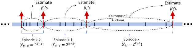
Figure 1: Schematic representation of the CORP policy. CORP has an episodic structure and updates its estimates of buyers’ preference vectors at the beginning of each episode. The estimates are computed via the maximum log-likelihood method using outcomes of auctions. The dark blue rectangles show the random exploration periods.

At the beginning of each episode $k$, we estimate the preference vectors of the buyers using the outcome of the auctions ($q_{it}$’s) in the previous episode, i.e., episode $k-1$, and we do not change our estimates during episode $k$. Let $\widehat{\beta}_{ik}$ be the estimated preference vector of buyer $i$ at the beginning of episode $k$. Then, $\widehat{\beta}_{ik}$ solves the following optimization problem:

$${\widehat{\beta}_{ik}}~{}=~{}\underset{\|\beta\|\leq B_{p}}{\arg\min\;}{{\cal L}_{ik}(\beta)},~{}~{}i\in[N]\,,$$ (8)

where

$${\cal L}_{ik}(\beta)~{}=~{}-\frac{1}{\ell_{k-1}}\sum_{t\in E_{k-1}}\Big{\{} q_{it}\log\big{(}(1-F(\max\{{b_{-it}^{+}},r_{it}\}-\langle x_{t},\beta\rangle))\big{)}$$

$$+(1-q_{it})\log\big{(}F(\max\{{b_{-it}^{+}},r_{it}\}-\langle x_{t},\beta\rangle)\big{)}\Big{\}}$$ (9)

is the negative of the log-likelihood function. Here, $b_{-it}^{+}$ refers to the maximum bids of buyers other than buyer $i$, in period $t$; that is, $b_{-it}^{+}=\max_{j\neq i}b_{jt}$. Then, buyer $i$ wins the auction in period $t$ if and only if $b_{it}>\max\{b_{-it}^{+},r_{it}\}$. Throughout the manuscript, to avoid ties, we make a simplifying assumption that the submitted bids are distinct. Similarly, we define $v_{-it}^{+}=\max_{j\neq i}v_{jt}$. Note that $F(\max\{{b_{-it}^{+}},r_{it}\}-\langle x_{t},\beta\rangle)$ is the probability of event $\langle x_{t},\beta\rangle+z_{it}\leq\max\{{b_{-it}^{+}},r_{it}\}$, which is the probability that buyer $i$ does not win the item at time $t$, upon bidding truthfully. The log-likelihood function ${\cal L}_{ik}(\beta)$ is computed after running the auctions in all the periods of episode $E_{k-1}$. Therefore, the firm has access to the required knowledge to compute the log-likelihood function ${\cal L}_{ik}(\beta)$. Specifically, by the time the firm computes ${\cal L}_{ik}(\beta)$, she has access to the submitted bids of the buyers in periods $t\in E_{k-1}$ as well as the reserve prices used in these periods.

Now, one may wonder why CORP does not use a simple mean square error estimator for which the estimate of preference vector $\beta_{i}$ at the beginning of episode $k$ is given by $\underset{\|\beta\|\leq B_{p}}{\arg\min\;}\sum_{t\in E_{k-1}}(b_{it}-\langle x_{t},\beta\rangle)^{2}$. This quadratic estimator, unlike the maximum Likelihood estimator used in CORP, uses the submitted bids of buyers directly and as a result, it is rather vulnerable to the strategic behavior of the buyers. This is so because the mean square error estimators are sensitive to outliers and this undesirable property would be an advantage to strategic buyers to manipulate the seller’s pricing policy. In light of this observation, to estimate the preference vector of any buyer $i$, CORP applies a maximum Likelihood estimator that only uses the outcome of the auctions $q_{it}$, that we refer to as “censored bids”, and submitted bids of other buyers expect buyer $i$; see the definition of the log-likelihood function in Equation (9). This makes the estimation procedure of the policy robust to untruthful bidding behavior of the buyers, as untruthful bidding may not necessarily lead to a different outcome. In addition, due to this feature of the learning policy, the buyers are incentivized to bid truthfully unless they are interested in changing the outcome of the auction at the expense of losing their current utility. Later when we outline the proof of the regret bound of CORP, we further elaborate on this.

After estimating the preference vectors at the beginning of each episode $k$, the policy proceeds to use its estimation to set reserve prices. In particular, the reserve price in period $t\in E_{k}$, $r_{it}$, solves

$$r_{it}~{}=~{}\underset{y}{\arg\max\;}\big{\{}y\big{(}1-F(y-{{\color[rgb]{0,0,0}{\langle x_{t},\widehat{\beta}_{ik}\rangle}}})\big{)}\big{\}}\,.$$ (10)

Note that by Proposition 3.1, if $\widehat{\beta}_{ik}=\beta_{i}$, then $r_{it}=r_{it}^{\star}$ where $r_{it}^{\star}$ is the optimal reserve price of buyer $i$ in period $t$.

CORP: A Contextual Robust Pricing Initialization: For any $k\in\mathbbm{Z}^{+}$, let $\ell_{k}=2^{k-1}$ and $E_{k}=\{\ell_{k},\dotsc,\ell_{k+1}-1\}$. Moreover, we let $r_{i1}=0$ and $\widehat{\beta}_{i1}=0$ for any $i\in[N]$. Updating Preference Vectors: At the start of each episode $k=1,2,\ldots$, i.e, at the beginning of period $t=\ell_{k}$, estimate the preference vectors, denoted by $\{\widehat{\beta}_{ik}\}_{i\in[N]}$, as follows $\displaystyle\widehat{\beta}_{ik}=\underset{\|\beta\|\leq B_{p}}{\arg\min\;}{\cal L}_{ik}(\beta),~{}~{}i\in[N]\,,$ (11) where ${\cal L}_{ik}(\beta)$ is defined in Equation (9). Setting Reserves: In each episode $k=1,2,\ldots$, and for any period $t$ in this episode, i.e., $t\in E_{k}$, - Exploration Phase: With probability $\frac{1}{\ell_{k}}$, choose one of the $N$ buyers uniformly at random and offer him the item at price of $r\sim\text{\sf uniform}(0,B)$, where $\text{\sf uniform}(0,B)$ is the uniform distribution in the range $[0,B]$. For other buyers, set their reserve prices to $\infty$. - Exploitation Phase: With probability $1-\frac{1}{\ell_{k}}$, observe the feature vector $x_{t}$ and set the reserve of each buyer $i\in[N]$ to $$r_{it}=\arg\max_{y}\big{\{}y\big{(}1-F(y-{{\color[rgb]{0,0,0}{\langle x_{t},\widehat{\beta}_{ik}\rangle}}})\big{)}\big{\}}\,.$$

Table 1 CORP Policy

We now discuss some of the important features of our policy.

• In each episode $k$, every period $t$ is assigned to exploitation with probability $1-{1}/{\ell_{k}}$, and is assigned to exploration with probability $1/\ell_{k}$. In the exploration periods, the firm chooses one of the buyers at random and allocates the item to him if his submitted bid is above a reserve price $r\sim\text{\sf uniform}(0,B)$ where $\text{\sf uniform}(0,B)$ is the uniform distribution in the range $[0,B]$. In exploitation periods, the firm exploits her current estimate of the preference vectors to set the reserve prices where the estimates are obtained by applying the MLE method to the outcomes of auctions in episode $k-1$.

  As stated earlier, in the exploration periods, we randomly choose prices. However, the firm does not crucially use this randomness to identify the best reserve prices. Recall that to set the reserve prices, the firm uses all the data points in the previous episode, not only the data points in the exploration periods. The main purpose of setting reserve prices randomly in the exploration periods is to motivate the buyers to be truthful. Note that the buyer does not know if in a given period $t$, the prices are set randomly. Thus, if he underbids in such a period, with a positive probability, he loses the opportunity to obtain a positive utility. Considering this and the fact that the buyers discount the future utilities, the randomized reserve prices incentivize the buyers to bid truthfully.

• Another important factors that makes the CORP policy robust is its episodic structure and impatience of buyers. In the CORP policy, submitted bids in episode $k$ are not used in setting reserve prices until the beginning of the episode $(k+1)$. Therefore, there is always a delay until buyers observe the effect of a bid on their reserves. Then, since buyers are impatient and maximize their discounted cumulative utility, they have less incentive to bid untruthfully. This is a salient property of the CORP policy that bounds the perpetual effect of each bid and, as we will see in the analysis, leads to robustness of the learning policy to the strategic behavior of buyers.

4.1 Regret Bound of the CORP Policy

We now state our main result on the regret of the CORP policy.

Theorem 4.1 (Regret Bound: Known Noise Distribution)

Suppose that Assumption 3 holds and the firm knows the market noise distribution $F$. Then, the T-period worst-case regret of the CORP policy is at most $O\left(Nd\left(\log(Td)\log(T)+\frac{\log^{2}(T)}{\log^{2}(1/\gamma)}\right)\right)$, where the regret is computed against the benchmark, defined in Proposition 3.1.

The regret bound of CORP presented in Theorem 4.1 consists of two terms $O(Nd\log(Td)\log(T)$ and $O\left(Nd\frac{\log^{2}(T)}{\log^{2}(1/\gamma)}\right)$. The first term of the regret bound is due to the estimation error in preference vectors; that is, this term exists even if buyers were not strategic. The second term is due to the strategic behavior of the buyers. Observe that the second term decreases as buyers get less patient; i.e., $\gamma$ gets smaller.

The proof of Theorem 4.1 is proved in Appendix 9. To bound the regret of our policy, we note that untruthful bidding has two undesirable effects for the firm. First of all, both overbidding and shading increase the estimation errors of the preference vectors and thus, consequently, introduce errors in the reserve prices set by the firm. Second of all, bidding untruthfully can lower the second highest submitted bid as well as the reserve price of the winner, and this reduces the firm’s revenue. By this observation, we divide the policy’s regret into two parts, where each part captures the negative consequences of one of the aforementioned effects.

To bound the regret associated with the first effect, in Proposition 9.1, we determine to which extent buyers’ “lies” impact the estimation errors of the preference vectors and the reserve prices. We say a buyer lies when his untruthful bid changes the outcome of the auction, $q_{it}$, for this buyer relative to the truthful bidding. That is, we say buyer $i$ lies in period $t$ if ${\mathbb{I}}(v_{it}>\max\{{b_{-it}^{+}},r_{it}\})\neq{\mathbb{I}}(b_{it}>\max\{{b_{-it}^{+}},r_{it}\})$ holds. Our notion of lies is inspired by our maximum Likelihood estimator used in CORP. To estimate the preference vector of any buyer $i$, the maximum Likelihood estimator, defined in (9), only uses the outcome of the auctions and submitted bids of other buyers expect buyer $i$. Thus, untruthful bidding can change our estimate of preference vector of buyer $i$ and consequently his reserve price only when he “lies”.

Having established the impact of lies, we then show that the number of times that a buyer lies in each episode is logarithmic in the length of the episode; see Proposition 9.2. This bound is derived using the property of our estimation method. As stated earlier, to influence the estimation of the preference vectors and reserve prices, buyers need to change the outcome of the auctions where such a change is costly for them as it can lead to utility loss. We then make use of the fact that buyers are utility-maximizer and discount the future to bound the number of lies. Precisely, to get this bound, we compare the long-term excess utility obtained from a lie with the instant utility loss that it causes. In particular, we derive a lower bound on the utility loss of the buyers in episode $k$ by focusing on the random exploration periods. Note that buyers are not aware whether a period is an exploration period. Thus, with a positive probability, any untruthful bid leads to a utility loss. We further derive an upper bound on the (future) utility gain of the untruthful bidding in episode $k$. Our upper bound is the total discounted utility that any buyer can hope to achieve in the next episodes. Thus, the bound includes potential future utility gains that a buyer can enjoy by manipulating other buyers’ strategy and their reserve prices. Then, by arguing that for any utility-maximizer buyer, the upper bound on the utility gain should be greater than or equal to the lower bound on the utility loss, we bound the number of lies of the buyer. By characterizing the impact of lies in Proposition 9.1 and bounding the number of lies in Proposition 9.2, we are able to bound the regret associated with the first effect, namely the gap between the posted reserves and the optimal ones.

To bound the regret associated with the second effect, we quantify the impact of bidding untruthfully on the second highest bids and reserve of the winner; see Lemma 9.3. When buyers bid untruthfully, the second highest bid may decrease. Further, the winner of the auction can change and this, in turn, can lower the reserve price of the winner. Any of these events will hurt the firm’s revenue. To quantify this impact, we upper bound the amount of underbidding and overbidding from each buyer using the fact that the buyer is utility-maximizer; see Proposition 9.2. To do so, we employ a similar argument that we used to bound the number of lies.

After characterizing the regret due to both effects, we bound the total regret during each episode, and show that the total regret is logarithmic in the length of the episode. The proof is completed by noting that there are $O(\log T)$ episodes up to time $T$, as the length of episodes doubles each time.

5 Knowledge of Market Noise Distribution

In the CORP policy, we assumed that the market noise distribution is known to the seller or can be estimated sufficiently well from side data. However, we do not always have this commodity in practice. Ideally, we prefer a pricing policy that uses such knowledge minimally, if at all. To relax this assumption, we consider setting where the market noise distribution is not fully known, but is believed to belong to a known ensemble of distributions:

• Unknown (Fixed) Distribution from a Known Location-scale Ensemble: Suppose that the unknown market noise distribution belongs to a known location-scale family of log-concave distributions. To recall, a log-scale family of distribution is a one that for a variable $Y$ belonging to this family, the distribution function of random variable $aY+b$ also belongs to this family. Some examples include Normal, Uniform, Exponential, Logistic, and Extreme value distribution, to name a few. We propose a policy that achieves a regret of $O\left(Nd\log(Td)\sqrt{T}+N^{2}d\Big{(}1+\frac{1}{\log^{2}(1/\gamma)}\Big{)}\log^{3}(T)\right)$. (In Appendix 7, we further show that even when buyers are not strategic, no other policy can have a regret better than $\Omega(\sqrt{T})$.) To design CORP-II, we adopt the MLE estimator in CORP to also estimate the parameters of the noise distribution as well as the preference vectors, and in this sense, we follow the path pursued in (Javanmard and Nazerzadeh 2019) for the case of the single, non-strategic buyer. We refer to Section 5.1 for the details.

• Unknown (Time-varying) Distribution from a Given Ambiguity Set: This is a more general setting where the noise distribution is unknown and time-varying, but belongs to a given ambiguity set of the log-concave distribution. In Section 5.2, we propose the so-called SCORP policy whose regret is of order $O\Big{(}N\sqrt{d\log(Td)}\;T^{2/3}+{{\color[rgb]{0,0,0}{\frac{N}{\log(1/\gamma)}\log(T)\;T^{1/3}}}}\Big{)}$.

5.1 Unknown Distribution from a Known Location-Scale Ensemble

Consider a location-scale class of distributions ${\cal F}$:

$${\cal F}\equiv\Big{\{}F_{m,\sigma}:\,m\in{\mathbb{R}},\,\sigma\in[\underline{\sigma},\bar{\sigma}],\,\underline{\sigma}>0,\,F_{m,\sigma}(x)=F((x-m)/\sigma)\Big{\}}\,,$$ (12)

where $F$ is a known log-concave distribution with mean zero and variance one. We assume that the noise distribution is $F_{m,\sigma}\in{\cal F}$, with unknown parameters $m$, $\sigma$, where $m$ and $\sigma^{2}$ respectively corresponds to the mean and the variance of the noise distribution. Without loss of generality, we can assume that $m=0$; otherwise, the mean of the noise term can be absorbed in the features as an intercept term. As an example, the set ${\cal F}$ can be class of uniform distribution with the support of $[-a,a]$ where $a\in[\underline{a},\bar{a}]$ is unknown and $\underline{a},\bar{a}>0$. As another example, the set ${\cal F}$ can be a class of (truncated) normal distributions with unknown standard deviation from an interval.

We let $\alpha_{0}\equiv 1/\sigma$ and in the model (1), we multiply both sides with $\alpha_{0}$. This leads to

$$\tilde{v}_{it}=\langle x_{t},\theta_{i}\rangle+\tilde{z}_{it},\quad i\in[N],\;\;t\geq 1\,,$$ (13)

where $\tilde{v}_{it}=\alpha_{0}v_{it}$, $\theta_{i}=\alpha_{0}\beta_{i}$ and $\tilde{z}_{it}=\alpha_{0}z_{it}$. Notably, distribution of $\tilde{z}_{it}$ is $F$. The valuation model (13) is similar to our previous model where the market noises were drawn from a known distribution $F$. For this setting, we propose a pricing policy, named CORP-II which is very similar to the CORP policy: It has an episodic structure, where the length of episodes grows exponentially, namely episode $k$ is of length $\ell_{k}=2^{k-1}$. The first $\lceil\sqrt{\ell_{k}}\rceil$ periods of episode $k$ are the pure exploration periods. In each of these period, a buyer is chosen in a round robin fashion (call him $i^{\circ}_{t}$) and offer him the item at price of $r_{t}\sim{{\sf uniform}}(0,B)$. For other buyers, we set their reserves to $\infty$. In the remaining periods of the episode, we set the reserve prices based on the current estimates of the preference vectors and the scale parameter $\alpha_{0}$. Specifically, we let $I_{k}$ be the set of pure exploration periods in episode $k$ (so $|I_{k}|=\lceil\sqrt{\ell_{k}}\rceil$) and form the negative log-likelihood function to estimate both $\beta_{i}$ and $\alpha_{0}$ using the outcomes of auctions in $I_{k}$:

$$\tilde{{\cal L}}_{ik}(\theta,\alpha)~{}=~{}-\Big{\lceil}\frac{N}{|I_{k}|}\Big{\rceil}\sum_{{\{t\in I_{k},i^{\circ}_{t}=i\}}}\Big{\{} q_{it}\log\left(1-F(\alpha r_{t}-\langle x_{t},\theta\rangle)\right)$$

$$+(1-q_{it})\log\left(F(\alpha r_{t}-\langle x_{t},\theta\rangle)\right)\Big{\}}\,.$$ (14)

The function $\tilde{\cal L}_{ik}$ is indeed the negative log-likelihood for allocation variables $q_{it}$ for $t\in I_{k}$, conditional on the feature vectors $x_{t}$, and the events $i^{\circ}_{t}=i$, $r_{it}=r_{t}$, assuming that buyer $i$ is truthful. The term $\lceil N/|I_{k}|\rceil$ comes from the fact that the buyer $i^{\circ}_{t}$ is chosen in a round robin fashion and so for a fixed $i$, there are $1/N$ fraction of the periods in $I_{k}$ contributing to the log-likelihood function $\tilde{\cal L}_{ik}$.

Let $(\widehat{\theta}_{ik},\widehat{\alpha}_{0k})$ solves the following optimization problem:

$$(\widehat{\theta}_{ik},\widehat{\alpha}_{0k})~{}=~{}\underset{\|(\theta,\alpha)\|\leq\tilde{B}_{p}}{\arg\min\;}{\tilde{{\cal L}}_{ik}(\theta,\alpha)},~{}~{}i\in[N]\,,$$ (15)

with $\tilde{B}_{p}=B_{p}+1/\underline{\sigma}$.

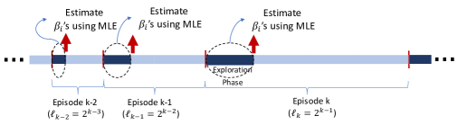
Figure 2: Schematic representation of the CORP-II policy. CORP-II has an episodic structure and updates its estimates of buyers’ preference vectors at the beginning of each episode. Each episode $k$ starts with a pure exploration phase $I_{k}$ of length $\lceil\ell_{k}^{1/2}\rceil$. CORP-II estimates preference vectors $\beta_{i}$ using MLE applied to the outcomes of auctions run in the previous pure exploration phase.

In the exploitation phase, the reserve of each buyer $i\in[N]$ is set to

$$r_{it}=\arg\max_{y}\,\{y(1-F(\widehat{\alpha}_{0k}y-\langle x_{t},\widehat{\theta}_{ik}\rangle)\}\,.$$ (16)

The formal description of CORP-II policy is given in Table 2. We also provide a schematic representation of CORP-II in Figure 2. CORP-II has a very similar structure to CORP. The main difference is that unlike CORP, we have some forced (pure) exploration periods at the beginning of each episode at which we experiment with random prices to learn both the preference vectors and the parameters of the noise distribution. The force exploration periods are required because in the current setting the market noise distribution is not fully known; see lower bound on regret in Appendix 7. By comparison, in CORP, the market noise distribution $F$ is fully known to the seller and we have much fewer of exploration periods (recall that in CORP, in each period of episode $k$, we do exploration with probability $1/\ell_{k}$ and so in expectation, we have only one exploration period in each episode).

CORP-II: A Contextual Robust Pricing Initialization: For any $k\in\mathbbm{Z}^{+}$, let $\ell_{k}=2^{k-1}$, $E_{k}=\{\ell_{k},\dotsc,\ell_{k+1}-1\}$, and $I_{k}=\{\ell_{k},\dotsc,\ell_{k}+\lceil\sqrt{\ell_{k}}\rceil\}$. Moreover, we let $r_{i1}=0$ and $\widehat{\beta}_{i1}=0$ for any $i\in[N]$. For $k=1,2,\dotsc$, do the following steps: Pure Exploration Phase: For $t\in I_{k}$, a buyer is chosen in a round robin fashion (call him $i^{\circ}_{t}$) and offer him the item at price of $r_{t}\sim{{\sf uniform}}(0,B)$. For other buyers, we set their reserves to $\infty$. Updating Estimates: At the end of the exploration phase, update the estimate of the preference vectors by applying MLE to the previous pure exploration phase: $\displaystyle(\widehat{\theta}_{ik},\widehat{\alpha}_{0k})=\underset{\|(\theta,\alpha)\|\leq\tilde{B}_{p}}{\arg\min\;}{\tilde{\cal L}}_{ik}(\theta,\alpha),~{}~{}i\in[N]\,,$ (17) where $\tilde{\cal L}_{ik}(\theta,\alpha)$ is given by Equation (14). Exploitation Phase: For other $t\in E_{k}$, observe the feature vector $x_{t}$ and set the reserve of each buyer $i\in[N]$ to $\displaystyle r_{it}=\underset{y}{\arg\max}\,\left\{y\big{(}1-F(\widehat{\alpha}_{0k}y-\langle x_{t},\widehat{\theta}_{ik}\rangle)\big{)}\right\}\,.$ (18)

Table 2 CORP-II Policy

Note that by the decoupling property (as stated in Proposition 3.1), the benchmark policy can focus on each buyer separately. This leads to the following optimal reserve, which optimizes the revenue obtained from buyer $i$:

$$r^{\star}_{i}(x)=\arg\max_{y}\,\{y(1-F(\alpha_{0}y-\langle x,\theta_{0}\rangle))\}\,.$$

Our next theorem characterizes the regret bound of CORP-II policy against a benchmark that knows the buyers’ preference vectors $\beta_{i}$ and the true market noise distribution.

Theorem 5.1 (Regret Bound: Unknown Noise Distribution from a Location-Scale Ensemble)

Consider the valuation model (1) where the market noise $z_{it}$’s are generated from a distribution belonging to ${\cal F}$, defined in (12). Suppose that $F$ in the definition of ${\cal F}$ satisfies Assumption 3. Then, the T-regret worst-case regret of CORP-II policy is at most

$$O\left(Nd\log(Td)\sqrt{T}+N^{2}d\Big{(}1+\frac{1}{\log^{2}(1/\gamma)}\Big{)}\log^{3}(T)\right)\,,$$

where the regret is computed against the clairvoyant that knows the buyers’ preference vectors $\beta_{i}$ and the noise distribution.

We refer to Appendix 10 for the proof of Theorem 5.1. Note that the extra regret due of the strategic behavior of the buyer is in the order of $O\left(\frac{dN^{2}\log^{3}(T)}{\log^{2}(1/\gamma)}\right)$. Interestingly, the extra regret scales only poly-logarithmically in $T$.

5.2 Unknown Distribution from a Given Ambiguity Set

The CORP policy presented in this paper is assumed to know the market noise distribution $F$. This knowledge is used in forming the log-likelihood estimator to learn preference vectors $\beta_{i}$’s and also in setting the reserves for buyers as in (10). Furthermore, we relaxed this assumption in the previous section by assuming that $F$ is unknown and fixed and belongs to a location–scale family, and for this setting, we presented CORP-II policy. Nevertheless, in practice, it may very well be the case that distribution $F$ is unknown and time-varying and as a result, it cannot be well approximated. To address this problem, we propose a variant of the CORP policy, called Stable Contextual Robust Pricing (SCORP), which is robust against the lack of knowledge of $F$. Specifically, we consider an ambiguity set ${\cal F}$ of possible probability distributions for the market noise and propose a policy that works well for every probability distribution in the ambiguity set.

We make the following assumption on the ambiguity set ${\cal F}$. This assumption is analogous to Assumption 3.

[Log-concavity of the Ambiguity Set ${\cal F}$] All functions $F\in{\cal F}$ are log-concave.

To be fair, in this case, we compare the regret of our policy against a benchmark policy, called robust, that knows the true preference vectors $\beta_{i}$ and the ambiguity set ${\cal F}$ that includes $F$, but is oblivious to distribution $F$ itself. The robust benchmark is defined as follows:

Definition 5.1 (Robust Benchmark)

In the robust benchmark, the reserve price of buyer $i\in[N]$ for a feature vector $x\in{\cal{X}}$ is given by

$$r^{\star}_{i}(x)=\underset{y}{\arg\max}\,~{}\underset{F\in{\cal F}}{\min}\,\left\{y\left(1-F(y-{{\color[rgb]{0,0,0}{\langle x,\beta_{i}\rangle}}})\right)\right\}\,,\quad i\in{[N]},\quad x\in{\cal{X}}\,,$$ (19)

and thus $r^{\star}_{it}=r^{\star}_{i}(x_{t})$ in this case.

The robust benchmark is motivated by our previous benchmark presented in Proposition 3.1. In our previous benchmark, we show that given a distribution $F$ and context $x$, the revenue-maximizing reserve price for buyer $i$ solves $r^{\star}_{i}(x)={\arg\max}_{y}\,\left\{y\left(1-F(y-{{\color[rgb]{0,0,0}{\langle x,\beta_{i}\rangle}}})\right)\right\}$. In the robust benchmark, the posted reserve prices have a similar form. However, the reserve prices which solves the optimization problem (19), are chosen in a robust way so that the benchmark performs well despite the uncertainty in the market noise distribution. We will discuss the complexity of optimization problem (19) in Section 5.2.1.

We note from the robust benchmark, as well as our learning policy, that we will present shortly do not aim at learning the distribution of market noise, as this distribution can vary across periods. For instance, in online advertising, the distribution of the noise can depend on many different factors including the time of the day and demographic information of the Internet users. Thus, instead of trying to learn the market noise distribution, we would like to use reserve prices that are robust to the uncertainty in the noise distribution.

We are now ready to present our SCORP policy. This policy is a modified version of the CORP-II policy. For reader’s convenience, we also provide a schematic representation of SCORP in Figure 3. Similar to the CORP-II policy, SCORP has an episodic theme, with the length of episodes growing exponentially. As before, we denote the set of periods in episode $k$ by $E_{k}$, i.e., $E_{k}=\{\ell_{k},\dotsc,\ell_{k+1}-1\}$, with $\ell_{k}=2^{k-1}$. Each episode $k$ starts with a pure exploration phase of length ${\lceil\ell_{k}^{2/3}\rceil}$. As before, we use notation $I_{k}$ to refer to periods in the pure exploration phase of episode $k$, i.e., $I_{k}=\{\ell_{k},\dotsc,\ell_{k}+{\lceil\ell_{k}^{2/3}\rceil}\}$. During each period in $I_{k}$, we choose one of the $N$ buyers uniformly at random and offer him the item at price of $r\sim{\sf uniform}(0,B)$. For other buyers, we set their reserve prices to $\infty$. Observe that in SCORP, because distribution $F$ is time-varying, we dedicate more periods to pure exploration than CORP-II. In the remaining periods of the episode (i.e., $E_{k}\backslash I_{k}$), we offer the reserve prices based on the current estimates of the preference vectors which are obtained by applying the least-square estimator to the outcomes of auctions in the pure exploration phase, $I_{k}$; see Equations (20) and (22). This is the exploitation phase as we set reserves based on our best guess of the preference vectors.

We note that the SCORP policy follows a similar structure to the LEAP policy proposed in Amin et al. (2014). Assuming that the time horizon $T$ is known, the LEAP policy designates the first $O(T^{2/3})$ periods to pure exploration and the remaining periods to exploitation. Using the doubling trick, the LEAP policy is extended to the setting with an unknown time horizon, which then admits a similar structure to SCORP. In comparison between SCORP and LEAP, it is worth highlighting a few points: 1) SCORP generalizes LEAP to the case of multi-buyers. 2) LEAP considers a setting with noiseless valuations while SCORP allows for noise component in the valuation function. As a consequence, the pricing functions differ in the two policies. SCORP uses (22), which involves a min-max optimization over the ambiguity set ${\cal F}$ while in LEAP, the prices in the exploitation periods are set as $p_{t}=\langle x,{\widehat{\theta}}\rangle-{\varepsilon}_{t}$, for an appropriate choice of ${\varepsilon}_{t}$. 3) More on the technical part, SCORP updates its estimate on the preference vectors only at the end of each exploration phase while LEAP update its estimate at each period by taking a gradient step on the prediction loss.

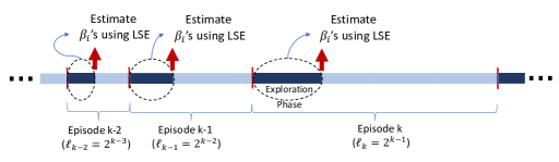
Figure 3: Schematic representation of the SCORP policy. SCORP has an episodic structure and updates its estimates of buyers’ preference vectors at the beginning of each episode. Each episode $k$ starts with a pure exploration phase $I_{k}$ of length $\lceil\ell_{k}^{2/3}\rceil$. SCORP estimates preference vectors $\beta_{i}$ using LSE applied to the outcomes of auctions run in the previous pure exploration phase.

The formal description of SCORP is given in Table 3.

SCORP: Stable Contextual Robust Pricing Policy Initialization: For any $k\in\mathbbm{Z}^{+}$, let $\ell_{k}=2^{k-1}$, $E_{k}=\{\ell_{k},\dotsc,\ell_{k+1}-1\}$, and $I_{k}=\{\ell_{k},\dotsc,\ell_{k}+{\lceil\ell_{k}^{2/3}\rceil}\}$. Moreover, we let $r_{i1}=0$ and ${{\color[rgb]{0,0,0}{\widehat{\beta}_{i1}}}}=0$ for any $i\in[N]$. For $k=1,2,\dotsc$, do the following steps: Pure Exploration Phase: For $t\in I_{k}$, choose one of the $N$ buyers uniformly at random and offer him the item at price of $r\sim\text{\sf uniform}(0,B)$. For other buyers, set their reserve prices to $\infty$. Updating Estimates: At the end of the exploration phase, update the estimate of the preference vectors by applying the least-square estimator to the previous pure exploration phase: $\displaystyle\widehat{\beta}_{ik}~{}=~{}\arg\min_{\|\beta\|\leq B_{p}}\tilde{\cal L}_{ik}(\beta),~{}~{}i\in[N]\,,$ (20) where $\tilde{\cal L}_{ik}(\beta)$ is given by $\displaystyle\tilde{\mathcal{L}}_{ik}(\beta)~{}=~{}\frac{1}{|I_{k}|}\sum_{t\in I_{k}}(BNq_{it}-\langle x_{t},\beta\rangle)^{2}\,.$ (21) Exploitation Phase: For $t\in E_{k}\backslash I_{k}$, observe the feature vector $x_{t}$ and set the reserve of each buyer $i\in[N]$ to $\displaystyle r_{it}=\underset{y}{\arg\max}\,~{}\underset{F\in{\cal F}}{\min}\,\left\{y\big{(}1-F(y-{{\color[rgb]{0,0,0}{\langle x_{t},\widehat{\beta}_{ik}\rangle}}})\big{)}\right\}\,.$ (22)

Table 3 SCORP Policy

Having presented our policy, we now highlight few important remarks about the estimation process of the policy. (i) Since the noise distribution is unknown and time-varying, SCORP  employs the least-square estimator (LSE) rather than the maximum Likelihood method, used in CORP and CORP-II; compare Equations (9) and (14) with (21). To apply the least-square estimator, similar to the CORP and CORP-II policies, SCORP uses the outcome of the auctions, not the submitted bids. In particular, SCORP minimizes the loss function $\tilde{\cal L}_{ik}(\beta)$ where the loss function is designed in a way to provide an unbiased estimator of the preference vectors under the truthful bidding strategy. To see why note that to estimate the preference vectors, we only use the outcome of the auctions, $q_{it}$, in the exploration periods $I_{k}$ where in exploration periods, the prices are chosen uniformly at random in $[0,B]$. Then, when buyers are truthful, the expectation of $BNq_{it}$ w.r.t. the randomness in prices and the noise in the valuations is ${\mathbb{E}}[BN\frac{1}{N}\Pr[v_{t}\geq r_{it}]|v_{t}]={\mathbb{E}}[v_{t}]=\langle x_{t},\beta\rangle$. This implies that under the truthful bidding strategy, the expectation of $BNq_{it}-\langle x_{t},\beta\rangle$ for any exploration period $t\in I_{k}$ is zero. Put differently, even under truthful bidding, the expectation of $BNq_{it}-\langle x_{t},\beta\rangle$ for exploitation periods $t\notin I_{k}$ is not zero and as a result, we only use the data in the exploration periods to estimate the preference vectors, and this, in turn, enforces the SCORP policy to dedicated $O(T^{2/3})$ periods to exploration. This makes SCORP robust to the strategic behavior of the buyers. (ii) Due to uncertainty in the noise distribution, for estimation, SCORP only utilizes the auction outcomes in the exploration phase where it does price experimentation. This is in contrast to CORP policy where all the auction outcomes in the previous episode are used to estimate the preference vectors. It is worth noting that in our analysis of the regret, we give up on the revenue collected during pure exploration phases and only use the outcomes of auctions in these phases to bound the estimation error of the preference vectors. (iii) So far, we argued SCORP is designed in a way to ensure robustness against strategic buyers. Importantly, we also note that the choice of reserve prices in the exploitation phase of SCORP makes this policy robust against the uncertainty in the noise distribution. Thus, SCORP  is indeed doubly robust.

Our next result upper bounds the regret of the SCORP  policy.

Theorem 0 (Regret Bound: Unknown Noise Distribution from an Ambiguity Set )

Suppose that Assumption 5.2 holds, and that the market noise distribution is unknown and belongs to uncertainty set ${\cal F}$. Then, the T-period worst-case regret of the SCORP  policy is at most

$$O\left(N\sqrt{d\log(Td)}\;T^{2/3}+{{\color[rgb]{0,0,0}{\frac{N}{\log(1/\gamma)}\log(T)\;T^{1/3}}}}\right)=O(N\sqrt{d\log(Td)}\;T^{2/3})\,,$$

where the regret is computed against the robust benchmark.

Observe that due to the strategic behavior of the buyers, the firm suffers from an extra regret of $O\left({{\color[rgb]{0,0,0}{\frac{N}{\log(1/\gamma)}\log(T)\;T^{1/3}}}}\right)$, where this regret shrinks as $\gamma$ decreases. We note that while the regret of the CORP-II policy is in the order of $O(d\log(Td)\sqrt{T})$, the regret of SCORP is $O(\sqrt{d\log(Td)}\,T^{2/3})$. The higher regret of SCORP is mostly due to the fact that distribution $F$ is time-varying, and because of this, SCORP cannot make use of the exploratory effect of the noise. Considering this, the SCORP policy dedicates more periods to exploration This implies that the SCORP policy learns preference vectors at a slower rate than CORP-II policy. The slower learning rate is the main reason behind the higher regret of SCORP.

The proof of Theorem 5.2 is provided in Appendix 11.

Remark 5.2

SCORP policy provides a very general machinery to design low-regret doubly robust learning policies, against different benchmarks. To make it clear, assume that firm uses a benchmark that posts reserve price of $r_{i}^{*}(x)=\rho(\langle x,\beta_{i}\rangle,{\cal F})$ for buyer $i$, under context vector $x\in{\cal{X}}$. Here, $\rho(\langle x,\beta_{i}\rangle,{\cal F})=\arg\max_{y}\min_{F\in{\cal F}}G(y,\langle x,\beta_{i}\rangle,F)$, where $G:{\mathbb{R}}\times{\mathbb{R}}\times{\cal F}\rightarrow\mathbb{R}$. Then, as long as $\rho(\langle x,\beta_{i}\rangle,{\cal F})$ is Lipschitz in its first argument, we can design a low-regret doubly robust learning policies against this benchmark by only changing the exploitation phase of the SCORP policy. Particularly, in a period $t$ in the exploitation phase of episode $k$, we set $r_{it}=\rho(\langle x,{\widehat{\beta}_{ik}}\rangle,{\cal F})$; see Equation (22) for comparison.

5.2.1 Complexity of SCORP

In SCORP, in each exploitation period, the optimization problem (22) needs to be solved to set reserve prices. Here, we discuss several cases where this optimization problem is rather easy to solve. We start by presenting an example in which the ambiguity set consists of uniform distributions. For this example, we provide a simple closed form solution for problem (22). We then discuss the uniform distributions are not exceptions in the sense that for many classes of distributions, the optimization problem of SCORP is indeed easy to solve.

Example 5.3 (Uniform Distributions)

Assume that the ambiguity set $\mathcal{F}$ includes all the uniform distributions with support of form $[-a,a]$ where $a\in[\underline{a},\bar{a}]$. The following theorem presents the optimal solution of problem (22) for the described $\mathcal{F}$. Before stating the theorem, let us stress again that in the setting of SCORP, the distribution $F\in{\cal F}$ can change over time. So, for this example it means that at step $t$, the market noises are drawn from a uniform distribution $F$, with support $[-a_{t},a_{t}]$, where $a_{t}\in[\underline{a},\bar{a}]$, is unknown and time varying.

Theorem 0

Suppose that $\mathcal{F}$ includes all the uniform distributions with the support of $[-a,a]$ where $a\in[\underline{a},\bar{a}]$. Then, for any $w$, we have

$$\underset{y}{\arg\max}\,~{}\underset{F\in{\cal F}}{\min}\,\left\{y\big{(}1-F(y-w)\big{)}\right\}=\left\{\begin{array}[]{ll}\frac{w+\underline{a}}{2}&~{}~{}\mbox{if $w\leq\underline{a}$};\\ w&~{}~{}\mbox{if $w\in(\underline{a},\bar{a})$};\\ \frac{w+\bar{a}}{2}&\mbox{if $w\geq\bar{a}$}.\end{array}\right.$$

The proof of the theorem is deferred to the appendix.

In Example 5.3, we observe that under uniform distributions, the robust optimization problem in (22) has a simple and easy-to-compute solution. This stems from the fact that the uniform distributions enjoy a single-crossing property; see Figure 4. To make it clear, let $F_{a}(\cdot)$ be the distribution of the uniform distribution in the range of $[-a,a]$ where $a>0$. Then, (i) for any $a$, $F_{a}(0)=\frac{1}{2}$, (ii) for any $y>0$ and $a>a^{\prime}$, $F_{a}(y)<F_{a^{\prime}}(y)$, and (iii) for any $y<0$ and $a>a^{\prime}$, $F_{a}(y)>F_{a^{\prime}}(y)$. That is, for any $a,a^{\prime}$, $F_{a}(\cdot)$ and $F_{a^{\prime}}(\cdot)$ cross each other once at $(0,1/2)$. Having this single-crossing property, the inner optimization problem in (22) is easy to solve and as a result, problem (22) has a closed form solution. We highlight that uniform distributions are not the only distributions that enjoy such a property. Consider normal distributions with mean zero and variance $\sigma^{2}$, denoted by $F_{\sigma}(\cdot)$. Then, for any $\sigma,\sigma^{\prime}$, $F_{\sigma}(\cdot)$ and $F_{\sigma^{\prime}}(\cdot)$ cross each other once at $(0,1/2)$. In general, the location-scale families (with fixed location parameter) considered in Section 5.1, namely ${\cal F}\equiv\{F_{\sigma}:\;\sigma\in[\underline{\sigma},\bar{\sigma}],\;\;\underline{\sigma}>0,\;F_{\sigma}=F(x/\sigma)\}$, satisfy the single-crossing property if $F$ is strictly increasing.

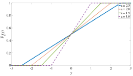
Figure 4: Single-crossing property for the uniform distributions.

6 Conclusion

Motivated by online marketplaces with highly differentiated products, we formulated a dynamic pricing problem in the contextual setting. In this problem, a firm runs repeated second-price auctions with reserve and the item to be sold in each period is described by a context (feature) vector. In our model, contextual information of an item influences buyers’ valuations of that item in a heterogeneous way, via buyers’ preference vectors. Due to the repeated interaction of buyers with the firm, buyers have the incentive to game the firm’s policy by bidding untruthfully. We proposed three pricing policies to set the reserve prices of buyers. These policies aim at learning the preference vectors of buyers in a robust way against the strategic behavior of buyers and meanwhile maximize the firm’s collected revenue.

The main insight behind the robustness property of our approach is that by an episodic design, we limit the long-term effect of each bid on the firm’s estimates of the preference vectors. Further, instead of using the bids (data) we use only the outcomes of auctions (censored data) in estimating preference vectors. Interestingly, we show that using this censored data does not hamper the learning rate while bringing in robustness property. As the granularity of real-time data increases at an unprecedented rate, we believe the ideas of this work can serve as a starting point for other complex dynamic contextual learning and decision making problems.

Authors’ Biographies

Negin Golrezaei. Negin Golrezaei is an Assistant Professor of Operations Management at the MIT Sloan School of Management. Her current research interests are in the area of machine learning, statistical learning theory, mechanism design, and optimization algorithms with applications to revenue management, pricing, and online markets. Before joining MIT, Negin spent a year as a postdoctoral fellow at Google Research in New York where she worked with the Market Algorithm team to develop, design, and test new mechanisms and algorithms for online marketplaces. She is the recipient of several awards including the 2018 Google Faculty Research Award; 2017 George B. Dantzig Dissertation Award; the INFORMS Revenue Management and Pricing Section Dissertation Prize; University of Southern California (USC) Ph.D. Achievement Award (2017), and USC Provost’s Ph.D. Fellowship (2011). Negin received her BSc (2007) and MSc (2009) degrees in electrical engineering from the Sharif University of Technology, Iran, and a Ph.D. (2017) in operations research from USC.

Adel Javanmard. Adel Javanmard is an Assistant Professor in the department of Data Sciences and Operations, Marshall School of Business at the University of Southern California. He also holds a courtesy appointment in the Computer Science Department within the USC Viterbi School of Engineering. Prior to joining USC in 2015, he obtained his Ph.D. in Electrical Engineering from Stanford University, followed by a postdoc at UC Berkeley and Stanford, supported by a fellowship from the NSF Center for Science of Information. Before that, he received BSc degrees in Electrical Engineering and Pure Math from Sharif University of Technology in 2009. His research interests are broadly in the area of high-dimensional statistical inference, machine learning and optimization. Adel is the recipient of several awards and fellowships, including the NSF CAREER award (2019), the Outlier Research in Business Award (2018), Dr. Douglas Basil Award for Junior Business Faculty (2018), the Zumberge Faculty Research and Innovation Fund (2017), Google Faculty Research Award (2016), the Thomas Cover dissertation award from the IEEE Society (2015), the CSoI Postdoctoral Fellowship (2015), the Caroline and Fabian Pease Stanford Graduate Fellowship (2010-2012).

Vahab Mirrokni. Vahab Mirrokni is a distinguished scientist, heading the New York and Zurich algorithms research groups at Google Research. The group consists of three main sub-teams: market algorithms, large-scale graph mining, and large-scale optimization. He received his Ph.D. from MIT in 2005 and his B.Sc. from the Sharif University of Technology in 2001. He joined Google Research in 2008, after spending a couple of years at Microsoft Research, MIT and Amazon.com. He is the co-winner of paper awards at KDD’15, ACM EC’08, and SODA’05. His research areas include algorithms, distributed and stochastic optimization, and computational economics. Recently he has been working on various algorithmic problems in machine learning, online optimization and dynamic mechanism design, and distributed algorithms for large-scale graph mining.

Regret Lower Bounds, Discussion, and Proof of Statements

7 Regret Lower Bounds

So far, we proposed three pricing policies (CORP, CORP-II, SCORP) for different settings of the problem (depending on how much information about the market noise distribution $F$ is available a priori to the seller). Here, we discuss various lower bounds for the regret of any pricing policy under different settings. This will shed light on the optimality gap of the proposed policies. In doing that, we focus on the simpler case of non-strategic (truthful) buyers. Nevertheless, we expect the same lower bounds carry over to the setting with strategic (utility maximizing) buyers because in such a setting, it would be even more challenging to the seller to design a low regret pricing policy.

7.1 Dependency on Time Horizon $T$

$\bullet$ Unknown $F$: Kleinberg and Leighton (2003) studied a single buyer non-contextual setting where the buyer’s valuation is drawn from an unknown random distribution $F$, and showed $\Omega(T^{2/3})$ lower bound. To show the lower bound, they focus on a family of distributions $\mathcal{F}=\{F_{j}^{T},j\in[K]\}$, where $K+1$ is the number of potential valuations and distribution $F_{j}^{T}$, $j\in[K]$, which depends on $T$, is obtained from perturbing the base distribution. Under the base distribution, posting any price leads to the same expected revenue while under distribution $F_{j}^{T}$, posting $(j+1)^{th}$ highest valuation as a price is optimal. In any period, buyer’s valuation is drawn from distribution $F_{j}^{T}$, $j\in[K]$, with probability $1/K$; that is, $F=F_{j}^{T}$ with probability $1/K$. For this setting, $\Omega({T^{2/3}})$ lower bound for the worst-case regret of any pricing policy is established, where the regret is computed against a clairvoyant policy that knows the realized valuation distribution in any period. We note that the lower bound obtained by Kleinberg and Leighton (2003) does not exactly fit into our framework. The reason is that Kleinberg and Leighton considered a benchmark that knows the valuation distributions while we consider a robust benchmark that hopes to do well for any distribution in the ambiguity set $\mathcal{F}$. That being said, we believe that this lower bound highlights the challenges in learning how to set optimal prices where market noise distribution is time varying, which is the setting we considered for the SCORP policy.

$\bullet$ Unknown $F$ from a Known Parametric Family: Broder and Rusmevichientong (2012) consider a single buyer setting, with a general parametric choice model and established $\Omega(\sqrt{T})$ lower bound for the worst-case regret of any pricing policy. The main idea is to construct specific problem class with a so-called “uninformative price”. Concretely, an uninformative price is a price such that all the demand curves (across the model parameters) intersect at that price. Such price impedes the demand learning because it does not reveal any information about the model parameter. Now, if the optimal price corresponding to a specific choice of model parameter is uninformative, then balancing the trade-off between exploration and exploitation results in the $\Omega(\sqrt{T})$ lower bound. When the optimal price can be uninformative, the policy can try to learn the model parameters fast by choosing prices that are sufficiently far from the uninformative price, but in doing that a large regret incurs because the policy is posting prices far from the optimal (an uninformative) price.

A similar trade-off is also used by Kleinberg and Leighton (2003) to establish lower bound for a single buyer non-contextual setting where the buyer’s valuation is drawn from an unknown distribution $F$. When the revenue function, i.e., $\text{Rev}(y)=y(1-F(y))$, has a unique global maximum, they established $\Omega(\sqrt{T})$ lower bound for the worst-case regret of any pricing policy. We note that when $F$ and $1-F$ are log-concave, the revenue function has a unique global maximum. The same property holds when $F$ is regular. To establish the lower bound, they consider a family of distributions parametrized by a single parameter such that no single price obtains a low regret with respect to all the distributions within the considered family. Similar to the setting when uninformative price exists, they show that to obtain a lower bound of $\Omega(\sqrt{T})$, the policy should post a price that is far from the optimal price, as by doing so, the learning rate increases.

In the following, we show that when the market noise distribution is known only up to a location–scale family (similar to the setting in Section 5.1), the uninformative prices do exist, even for settings with a single buyer, and hence following the same argument of Broder and Rusmevichientong (2012), we have $\Omega(\sqrt{T})$ lower bound for the regret of any pricing policy. To see this, consider $N=1$ and suppose that the feature vectors $x_{t}$ are drawn i.i.d. from a distribution that always takes the value of one on the first entry ($x_{t,1}=1$ for all $t$, denoting the intercept of the model). Let ${\cal F}$ be the known location-scale class of distributions given by (12), with $m=0$, namely

$${\cal F}\equiv\Big{\{}F_{\sigma}:\;\sigma\in[\underline{\sigma},\bar{\sigma}],\;\;\underline{\sigma}>0,\;F_{\sigma}=F(x/\sigma)\Big{\}}\,.$$

Fix an arbitrary $\eta$ such that $f(\eta)\neq 0$ and define $b_{0}$ and $b_{1}$ as

$$b_{0}=\frac{1-F(\eta)}{f(\eta)}\,,\quad\quad b_{1}=\frac{1-F(\eta)}{f(\eta)}-\eta\,.$$

Note that $b_{0}$ and $b_{1}$ are fixed. We consider preference vector $\beta=(b,0)\in{\mathbb{R}}^{d}$, with varying coefficient $b\in{\mathbb{R}}$. Further, consider the scaling parameter $\sigma=(b_{0}-b_{1}+b)^{-1}$ (see definition of family of distributions ${\cal F}$). Looking at the probability of purchase $1-F(\tfrac{r}{\sigma}-\langle x_{t},\beta\rangle)=1-F(\tfrac{r}{\sigma}-b)$, we see that $r=1$ is an uninformative price because the demand curves ${{\rm d}}(r,b):=1-F(\tfrac{r}{\sigma}-b)$ intersect at $1-F(b_{0}-b_{1})$ at price $r=1$ and hence this price does not give any information about the value of model coefficient $b$. On the other side, it is straightforward to see that $r=1$ is the optimal price when $b=b_{1}$ (i.e, the derivative of the revenue $r\times{{\rm d}}(r,b_{1})$ vanishes at $r=1$). This shows that under this setting, we have uninformative prices that are indeed optimal for a specific choice of model parameters.

Comparing the regret of CORP-II with the $\Omega(\sqrt{T})$ lower bound indicates optimality of its regret (in terms of $T$), up to a logarithmic factor.

$\bullet$ Known Distribution $F$: In constructing the uninformative prices in the previous case, we used the fact that the scaling parameter $a$ of the distribution was unknown. (Recall that $a$ depended on the unknown coefficient $b$.) When the market noise distribution is fully known to the firm, then as we saw in the design of CORP, the firm can harness the randomness of the noise and use it to get free exploration of the demand parameters (by forming the log likelihood function), without having to actively randomize the prices. In such a setting, one can prove a lower bound of $\Omega(d\log T)$ by using the Van Trees inequality. (This approach is classic and we spare the details. We refer the interested reader to  Broder and Rusmevichientong (2012) or Goldenshluger and Zeevi (2013) for further details on this approach.) At a high level, the idea is to first lower bound the regret in period $t$ in terms of the mismatch between the posted price $r_{it}$ by the policy, and the optimal price $r^{\star}_{it}$, namely $(r_{it}-r^{\star}_{it})^{2}$. Then, treating $r^{\star}_{it}$ as a function of $\langle x_{t},\beta\rangle$, i.e., $r^{\star}_{it}=g(\langle x_{t},\beta_{i}\rangle)$ with $g(y)\equiv\arg\max_{y}y(1-F(y-\langle x_{t},\beta\rangle))$, one can apply the Van Trees inequality to establish a lower bound of $d/t$ for $(r_{it}-r^{\star}_{it})^{2}$, which results in a lower bound of $\Omega(d\log T)$ for the total regret incurred on horizon $T$. This approach has been followed in Broder and Rusmevichientong (2012) for a low-dimensional model (with single scalar parameter) to prove $\Omega(\log T)$ lower bound. However, this approach can be extended to feature-based models using a multi-dimensional version of Van Trees inequality (Gill et al. 1995) to get $\Omega(d\log T)$ lower bound.

Another approach to achieve the same lower bound of $\Omega(d\log T)$ is to relate the regret in each period to the minimax $\ell_{2}$ risk of estimating preference vectors, and then by following the Le Cam’s method (Tsybakov 2008), relate it to the error in a multi-way hypothesis problem defined over a packing set of the parameter space. This error, in turn, can be lower bounded using the Fano’s inequality from information theory. This type of argument to derive lower bound for minimax risks is quite standard in statistics; see, for example, Raskutti et al. (2011), Zhang et al. (2010), and Loh (2017). In (Javanmard and Nazerzadeh 2019, Theorem 5), the authors pursued this path for the setting of a single truthful buyer with sparse preference vector and established a lower bound of $\Omega(s_{0}\log(T/s_{0}))$, where $s_{0}$ denotes the number of nonzero entries for the preference vector. Setting $s_{0}=d$, this yields the $\Omega(d\log(T/d))$ lower bound for a general (non-sparse) preference vector.

Recall that our proposed CORP policy achieves a regret of $O(d\log(Td)\log(T))$. Comparing this with the above lower bound implies that CORP is optimal up to a logarithmic factor.

7.2 Dependency on Feature Dimension $d$

When talking about the dependency of the regret on the feature dimension $d$, we should also consider its dependency on $T$. For example, a naive policy that always posts random reserves, will get a regret of $O(T)$, without any dependency on the dimension $d$. The regret bounds we proved for CORP and CORP-II scale as $O(d\log d)$ in terms of the feature dimension $d$ and the regret of SCORP scales as $O(\sqrt{d\log d})$. Note that a linear dependency on $d$ is inevitable when the regret scales logarithmically in $T$. Indeed, as discussed in Section 7.1, we have a lower bound $\Omega(d\log T)$ for the case of single truthful buyer and assuming that the market noise distribution $F$ is fully known to the firm. Somewhat related, Lobel et al. (2016) studied a pricing problem in a single buyer setting with a contextual and noise-less valuation model, where contexts are chosen by an adversary. They show a lower bound of $\Omega(d\log(1/\epsilon\sqrt{d}))$ to obtain prices that are $\epsilon$ away from the optimal prices.

8 Discussion

In Section 8.1, we discuss how our polices can be extended to a setting with some of the nonlinear valuation models. We then discuss pricing with perishable data in Section 8.2.

8.1 Beyond the Linear Valuation Model

In this paper, we focused on linear valuation model (1), where a buyer’s valuation of a product is a linear function of the product feature with an additive noise. The linear feature-based model is already rich enough to capture interesting interplay between the buyers and the firm and the main components of the dynamic pricing problem. That said, it is quite straightforward to generalize our analysis to some of the nonlinear valuation models. Concretely, consider the following model

$$v_{it}(x_{t})=\psi(\langle\phi(x_{t}),\beta_{i}\rangle+z_{it})~{}~{}~{}~{}~{}i\in[N],~{}t\geq 1\,.$$ (23)

where $\phi:{\mathbb{R}}^{d}\mapsto{\mathbb{R}}^{d}$ is a feature mapping and $\psi:{\mathbb{R}}\mapsto{\mathbb{R}}$ is a general strictly increasing function. Some examples of such models are: (i) Log-log model ($\psi(x)=e^{x},\phi(x)=\ln(x)$); (ii) Semi-log model $(\psi(x)=e^{x},\phi(x)=x)$; (iii) Logistic model $(\psi(x)=e^{x}/(1+e^{x})$, $\phi(x)=x)$.

Note that we can treat $\tilde{x}_{t}\equiv\phi(x_{t})$ as new features. Moreover, by the change of variable $\tilde{v}_{it}=\psi^{-1}(v_{it})$, we arrive at the valuation model $\tilde{v}_{it}=\langle\tilde{x}_{t},\beta_{i}\rangle+z_{it}$, which is the same as the linear model (1) studied in this work. Letting $\tilde{b}_{it}=\psi^{-1}(b_{it})$ and $\tilde{r}_{it}=\psi^{-1}(r_{it})$, the negative log-likelihood function for the preference vector $\beta$ given the outcome of the auctions $q_{it}$ reads as

$${\cal L}_{ik}(\beta)~{}=~{}-\frac{1}{\ell_{k-1}}\sum_{t\in E_{k-1}}\Big{\{} q_{it}\log\big{(}(1-F(\max\{\tilde{b}^{+}_{-it},\tilde{r}_{it}\}-\langle\tilde{x}_{t},\beta\rangle))\big{)}$$

$$+(1-q_{it})\log\big{(}F(\max\{\tilde{b}^{+}_{-it},\tilde{r}_{it}\}-\langle\tilde{x}_{t},\beta\rangle)\big{)}\Big{\}}\,,$$ (24)

with $\tilde{b}^{+}_{-it}=\max_{j\neq i}\tilde{b}_{jt}$.

Hence, in adopting the CORP policy to the nonlinear setting, we estimate preference vectors $\beta_{i}$ as

$${\widehat{\beta}_{ik}}~{}=~{}\underset{\|\beta\|\leq B_{p}}{\arg\min\;}{{\cal L}_{ik}(\beta)},~{}~{}i\in[N]\,,$$ (25)

with ${{\cal L}_{ik}(\beta)}$ given by (24).

To understand the benchmark reserves, note that similar to Proposition 3.1, the decoupling principle applies and $r^{\star}_{it}$ solves the following optimization problem

$$r^{\star}_{it} =\arg\max_{y}\{y\cdot$$

$$=\arg\max_{y}\{y\cdot$$

Therefore, the exploitation phase of the CORP policy should be modified as follows. Given the estimated preference vector $\widehat{\beta}_{ik}$, the reserve price of each buyer $i\in[N]$ is set as

$$r_{it}=\arg\max_{y}\;\;y(1-F(\psi^{-1}(y)-\langle\tilde{x}_{t},\beta_{i}\rangle))\,.$$

With these modifications, our analysis of CORP policy for linear valuation model carries over to the nonlinear model (23), establishing the $T$-period worst-case regret of $O\left(Nd\left(\log(Td)\log(T)+\frac{\log^{2}(T)}{\log^{2}(1/\gamma)}\right)\right)$.

8.2 Perishability of Data and Varying Coefficient Valuation Model

As discussed in CORP, CORP-II, and SCORP policies, the estimated preference vectors are updated in an episodic manner with the lengths of episodes growing over time. The rationale is that as the policy proceeds, the estimates get more accurate and hence they will be used over a longer episode.

In practice, however, due to the temporal behavior of buyers, their preference vectors may vary over time and hence the historical sale data is perished after a while to be used for estimating buyer’s valuation model. In such applications, it is not wise to stay with an estimated preference vector for a long time because the true preference vector may change significantly over this time frame. Time-varying demand environments have also been studied recently in the literature; see e.g. Keskin and Zeevi (2016) and Javanmard (2017), where they are modeled via varying-coefficient demand models. For example, Keskin and Zeevi (2016) considers the setting where a firm is selling one type of product to customers arriving over time. Following a price $p_{t}$, the firm observes demand $D_{t}=\alpha_{t}+\beta_{t}p_{t}+z_{t}$, where $\alpha_{t}$, $\beta_{t}\in{\mathbb{R}}$ are unknown model parameters and $z_{t}$ is the unobserved demand noise. The authors consider both smooth and bursty changes in a demand environment. For the case of smooth changes, they propose a weighted least squares estimation procedure that discounts older observations at an (asymptotically) optimal rate, whereas for the case of bursty changes, they develop a joint pricing and detection policy that continuously test if there has been a significant change in the environment.

Closer to the spirit of our work, Javanmard (2017) considers a feature-based valuation model with varying coefficient model for the case of a single non-strategic buyer. This work proposes a pricing policy based on projected gradient descent that update its estimate of the model parameters at every step as the information accrues to keep up with the possible volatility in the model parameters. The regret of the policy is characterized against a clairvoyant policy that knows the sequence of the model parameters in advance, and in terms of the time, feature dimension, as well as the temporal variability of the model parameters.

Extending our setting to the case of time-varying valuation model requires substantially different algorithms that update the estimates of the model parameters frequently. This is beyond the scope of the current work and is indeed the subject of a future work.

9 Proof of Theorem 4.1

The regret of the CORP policy is the sum of its regret across all episodes. Thus, in the following, we compute the regret incurred during an episode $k>1$. (The regret of episode $1$ that has a length of $1$ is a constant.)

We start with a definition. Let

$${{l_{F}}=\inf_{|x|\leq B_{n}}\left\{\min\left\{-\log^{\prime\prime}F(x),-\log^{\prime\prime}(1-F(x))\right\}\right\}\,,}$$ (26)

where $\log^{\prime\prime}F(x)=\frac{d^{2}}{dx^{2}}(\log(F(x)))$ and $\log^{\prime\prime}(1-F(x))=\frac{d^{2}}{dx^{2}}(\log(1-F(x)))$. Note that ${l_{F}}$ is a measure of “flatness” of function $\log F$. Because of log-concavity of $F$ and $1-F$ (cf. Assumption 3), we have ${l_{F}}>0$.

Recall that in the CORP policy, at the beginning of each episode $k>1$, the preference vectors $\beta_{i}$ are estimated via optimizing the log-likelihood function corresponding to the outcomes of auctions in the previous episode; see Equation (8). Now, consider buyer $i$ that bids untruthfully in period $t\in E_{k-1}$. Assume for the moment that bids of other buyers in this period are fixed. Then, the untruthful bid of buyer $i$ in period $t\in E_{k-1}$ may influence the estimation of his preference vector in episode $k$ only when his untruthful bid changes the allocation of the item in this period, i.e., ${\mathbb{I}}(v_{it}>\max\{{b_{-it}^{+}},r_{it}\})\neq{\mathbb{I}}(b_{it}>\max\{{b_{-it}^{+}},r_{it}\})$. This is the case because the preference vectors are estimated using the outcome of the auctions and not the submitted bids. When ${\mathbb{I}}(v_{it}>\max\{{b_{-it}^{+}},r_{it}\})\neq{\mathbb{I}}(b_{it}>\max\{{b_{-it}^{+}},r_{it}\})$ holds, we say buyer $i$ “lies” in period $t$. For each buyer $i\in[N]$, we further define the set of “lies” in episode $k-1$, indicated by ${\sf L}_{ik}$, as follows:

$${\sf L}_{ik}=\Big{\{}t:~{}t\in E_{k-1},\,{\mathbb{I}}(v_{it}>\max\{b_{-it}^{+},r_{it}\})\neq{\mathbb{I}}(b_{it}>\max\{b_{-it}^{+},r_{it}\})\Big{\}}\,.$$ (27)

In other words, ${\sf L}_{ik}$ consists of all the periods in episode $k-1$ in which buyer $i$ lies. We note that the set of lies in episode $k-1$, ${\sf L}_{ik}$, depends on the reserve prices $r_{it}$, $t\in E_{k-1}$, where the reserve prices are (mostly) set using the outcome of the auctions in episode $k-2$. Because of this dependency, ${\sf L}_{ik}$ may also depend on all the submitted bids in episodes $1,2,\ldots,k-1$. However, we will show that regardless of the values of $r_{it}$’s, the size of ${\sf L}_{ik}$ is logarithmic in the length of episode $k-1$; see Proposition 9.2.

Next, we quantify the adverse effect of lies on the firm’s estimates of the preference vectors. In particular, the next proposition provides an upper bound on the estimation error of $\widehat{\beta}_{ik}$ in terms of the number of samples used in the log-likelihood function ($\ell_{k-1}$), the dimension of the feature vector $(d)$, and the number of lies $(|L_{ik}|)$. Proof of Proposition 9.1 is deferred to Section 13.

Proposition 9.1 (Impact of Lies on Estimated Preference Vectors)

Let $\widehat{\beta}_{ik}$ be the solution of the optimization problem (8). Then, under Assumption 3, there exist constants $c_{0}$, $c_{1}$, and $c_{2}$ such that for $\ell_{k-1}\geq c_{0}d$, with probability at least $1-d^{-0.5}\ell_{k-1}^{-1.5}-2e^{-{c_{2}}\ell_{k-1}}$, we have

$$\|\widehat{\beta}_{ik}-\beta_{i}\|^{2}\leq\frac{c_{1}{{\color[rgb]{0,0,0}{d^{2}}}}}{{l_{F}}^{2}}\left(\left(\frac{|{\sf L}_{ik}|}{\ell_{k-1}}\right)^{2}+\frac{\log(\ell_{k-1}d)}{\ell_{k-1}}\right)\quad i\in[N]\,,$$ (28)

where ${l_{F}}$ is defined in Equation (26).

We note that the estimation error of $\widehat{\beta}_{ik}$’s affects the firm’s regret, as reserve prices are set based on these estimates. By Proposition 9.1, to keep our estimation errors small, the buyers should not have the incentive to lie in too many periods. In the next proposition, we show that for each episode $k$, the number of lies from a buyer is at most logarithmic in the length of the episode.

There is another way that bidding untruthfully can impact the firm’s regret. Recall that in each period $t$, the firm collects the revenue of $\max\{b_{t}^{-},r_{t}^{+}\}$ if the highest buyer clears his reserve. Then, by bidding untruthfully, the second highest bid $b_{t}^{-}$ may go down. Further, the winner can change, and this, in turn, can lower reserve price of the winner, $r_{t}^{+}$. To bound this impact of untruthful bidding, in the following proposition we bound the amount of underbidding from buyers who do not win an auction and the amount of overbidding from buyers who win an auction. Precisely, we show that the total amount of underbidding from each buyer $i$, in all periods $t\in E_{k}$ that he does not win the auction, is at most logarithmic in the length of that episode. We further show that the total amount of overbidding from each buyer $i$, in all periods $t\in E_{k}$ that he wins the auction, is at most logarithmic in the length of that episode.

Proposition 9.2 (Bounding the Number of Lies)

Denote by $s_{it}$ and $o_{it}$ the amount of shading and overbidding from buyer $i\in[N]$ in period $t$, i.e., $s_{it}=(v_{it}-b_{it})_{+}$, and $o_{it}=(b_{it}-v_{it})_{+}$, where $(y)_{+}$ is $y$ when $y\geq 0$ and zero otherwise. Then, there exist constants $c_{3},c_{4},\ldots,c_{9}$, such that for any fixed $0\leq\delta\leq 1$, with probability at least $1-(\delta+1)/\ell_{k-1}$, the following holds:

$$|{\sf L}_{ik}|~{}\leq~{}c_{3}\log(\ell_{k-1}/\delta)+{{\color[rgb]{0,0,0}{c_{4}\frac{\log(\ell_{k-1})}{\log(1/\gamma)}+c_{5}\frac{\log(N)}{\log(1/\gamma)}}}}\quad i\in[N]\,.$$ (29)

Further, we have that with probability at least $1-1/\ell_{k-1}$,

$$\sum_{{t\in E_{k-1}}}s_{it}(1-q_{it})~{} \leq~{}{{\color[rgb]{0,0,0}{c_{6}\frac{\log(\ell_{k-1})}{\log(1/\gamma)}+c_{7}\frac{\log(N)}{\log(1/\gamma)}}}}\quad{i\in[N]}\,,$$ (30)

$$\sum_{{t\in E_{k-1}}}o_{it}q_{it}~{} \leq~{}{{\color[rgb]{0,0,0}{c_{8}\frac{\log(\ell_{k-1})}{\log(1/\gamma)}+c_{9}\frac{\log(N)}{\log(1/\gamma)}}}}\quad{i\in[N]}\,.$$ (31)

Proof of Proposition 9.2 is given in Section 14. The main idea of the proof is to compute the excess utility that a strategic buyer can earn in the next episodes by bidding untruthfully in the current episode, and compare it with the utility loss that he suffers in the current episode because of his strategic behavior. The result then follows by using the fact that for a utility-maximizing buyer, the net excess utility should be nonnegative.

Up to here, we have established the impact of lies on our estimation, bounded the number of lies and the amount of underbidding from buyers. Next, using these results, we present a lower bound on the expected revenue of our policy in any period $t\in E_{k}$. We drop the superscript $\pi$ in our notation as it is clear from the context.

For each period $t$, we define a random variable $\xi_{t}$ that takes values in $\{0,1\}$, with $\xi_{t}=1$ if the firm is in the exploitation phase and $\xi_{t}=0$ otherwise. From the description of our policy, for any period $t$ in episode $k$, ($t\in E_{k}$), we have . We first lower bound the firm’s expected revenue in an exploitation period $t\in E_{k}$. Recall that in an exploitation period, the firm runs a second-price auction with reserve. Thus, we have

$${\sf{rev}}_{t}~{}\geq~{}$$ (32)

where the expectation is w.r.t. the randomness in the submitted bids. Since in each period $t$, at most one of the buyers gets the item, we can rewrite (32) as follows:

$${\sf{rev}}_{t} ~{}\geq~{}$$

$$~{}=~{}{\big{(}1-\frac{1}{\ell_{k}}\big{)}}\sum_{i=1}^{N}{\mathbb{E}}\left[\max\{b_{t}^{-},r_{it}\}{\mathbb{I}}(b_{it}>\max\{b_{t}^{-},r_{it}\})\right]\,.$$

Next, we compare ${\sf{rev}}_{t}$ with the expected revenue of the benchmark in period $t$, ${\sf{rev}}^{\star}_{t}$. Recalling (5), we have

$${\sf{rev}}^{\star}_{t}~{}=~{}\sum_{i=1}^{N}{\mathbb{E}}\left[\max\{v_{t}^{-},r^{\star}_{it}\}{\mathbb{I}}(v_{it}>\max\{v_{t}^{-},r^{\star}_{it}\})\right]\,.$$ (33)

Therefore, the regret of the policy in period $t$ can be upper bounded as

$${\sf{rev}}^{\star}_{t}-{\sf{rev}}_{t}~{}\leq~{}{\big{(}\frac{1}{\ell_{k}}\big{)}}{\sf{rev}}^{\star}_{t}$$

$$+{{\big{(}1-\frac{1}{\ell_{k}}\big{)}}}\sum_{i=1}^{N}{\mathbb{E}}\bigg{[}\max\{v_{t}^{-},r^{\star}_{it}\}{\mathbb{I}}(v_{it}>\max\{v_{t}^{-},r^{\star}_{it}\})-\max\{b_{t}^{-},r_{it}\}{\mathbb{I}}(b_{it}>\max\{b_{t}^{-},r_{it}\})\bigg{]}$$

$$~{}\leq~{}{\big{(}\frac{B}{\ell_{k}}\big{)}}+{{\big{(}1-\frac{1}{\ell_{k}}\big{)}}}\sum_{i=1}^{N}{\mathbb{E}}\bigg{[}\max\{v_{t}^{-},r^{\star}_{it}\}{\mathbb{I}}(v_{it}>\max\{v_{t}^{-},r^{\star}_{it}\})-\max\{b_{t}^{-},r_{it}\}{\mathbb{I}}(b_{it}>\max\{b_{t}^{-},r_{it}\})\bigg{]}\,,$$ (34)

where in the last equation, we used the fact that ${\sf{rev}}^{\star}_{t}\leq B$. We break down the second expression in  (34) into two terms:

$$\Delta_{1,t} = \sum_{i=1}^{N}\bigg{[}\max\{v_{t}^{-},r^{\star}_{it}\}{\mathbb{I}}(v_{it}>\max\{v_{t}^{-},r^{\star}_{it}\})-\max\{v_{t}^{-},r_{it}\}{\mathbb{I}}(v_{it}>\max\{v_{t}^{-},r_{it}\})\bigg{]}\,,$$ (35)

$$\Delta_{2,t} = \sum_{i=1}^{N}\bigg{[}\max\{v_{t}^{-},r_{it}\}{\mathbb{I}}(v_{it}>\max\{v_{t}^{-},r_{it}\})-\max\{b_{t}^{-},r_{it}\}{\mathbb{I}}(b_{it}>\max\{b_{t}^{-},r_{it}\})\bigg{]}\,.\;$$ (36)

Using our notation, Equation (34) can be rewritten as:

$${\sf{rev}}^{\star}_{t}-{\sf{rev}}_{t}\leq{\frac{B}{\ell_{k}}}+{{\big{(}1-\frac{1}{\ell_{k}}\big{)}}}{\mathbb{E}}[\Delta_{1,t}+\Delta_{2,t}]\,.$$ (37)

In the sequel, we will bound each term $\Delta_{1,t}$ and $\Delta_{2,t}$ separately. But before proceeding, let us pause to explain these terms and the intuition behind their definition. The regret of the firm’s policy is due to two factors:

1. Mismatch between $\boldsymbol{\beta}_{i}$ and $\boldsymbol{\widehat{\beta}}_{ik}$: The mismatch between the true preference vectors $\beta_{i}$ and the estimation $\widehat{\beta}_{ik}$ leads to a difference between the benchmark reserves ($r^{\star}_{it}$) and the posted reserves by the firm ($r_{it}$). The term $\Delta_{1,t}$ captures this factor and its effect on the regret. We will use Proposition 9.1 along with our first result in Proposition 9.2 to bound $\Delta_{1,t}$.

2. Mismatch between $\boldsymbol{v}_{t}^{-}$ and $\boldsymbol{b}_{t}^{-}$ and change of the winner: Note that the benchmark revenue ${\sf{rev}}^{\star}_{t}$ is measured against truthful buyers, while the firm’s revenue under our policy is measured against strategic buyers. The strategic behavior of buyers not only affects the quality of estimates $\widehat{\beta}_{ik}$ (and therefore the reserves $r_{it}$) but it may also affect the firm’s revenue via another quite subtle factor. Indeed, due to the strategic behavior of buyers, the second highest bid might go down or the winner of the auction might change from the case of truthful buyers and this may decrease the reserve of the winner. The decrease in the second highest bid or the reserve price of the winner can hurt the firm’s revenue. The term $\Delta_{2,t}$ captures these effects. We will use our second result in Proposition 9.2 to bound $\Delta_{2,t}$.

Bounding $\boldsymbol{\Delta_{1,t}}$: We now move to bounding $\Delta_{1,t}$. Recall that

$${\mathbb{E}}[\Delta_{1,t}]~{}= \sum_{i=1}^{N}{\mathbb{E}}\bigg{[}\max\{v_{t}^{-},r^{\star}_{it}\}{\mathbb{I}}(v_{it}>\max\{v_{t}^{-},r^{\star}_{it}\})-\max\{v_{t}^{-},r_{it}\}{\mathbb{I}}(v_{it}>\max\{v_{t}^{-},r_{it}\})\bigg{]}\,.$$

Here, the expectation is w.r.t. the randomness in the buyers’ valuations and potential randomness in reserve prices $r_{it}$ and $r^{\star}_{it}$. Note that the first expression inside the summation denotes the firm’s revenue when buyer $i$ wins the auction with reserve $r^{\star}_{it}$, while the second expression is the analogous term when the buyer $i$’s reserve is $r_{it}$. Further, conditional on the feature vector $x_{t}$, reserves $r^{\star}_{it}$ and $r_{it}$ are independent of $v_{t}^{-}$, and the right-hand side of the last equation can be written in terms of function $W_{it}(r)$, defined below:

$$W_{it}(r)~{}\equiv~{}{\mathbb{E}}\Big{[}\max\{v_{t}^{-},r\}{\mathbb{I}}(v_{it}\geq\max\{v_{t}^{-},r\})\Big{|}x_{t}\Big{]}\,,$$ (38)

where the expectation is with respect to valuation noises, conditional on $x_{t}$. By the law of iterated expectation, we can write ${\mathbb{E}}[\Delta_{1,t}]$ in terms of $W_{it}(r)$. More specifically, we first take the expectation conditional on $x_{t}$ and then take the expectation w.r.t. $x_{t}$.

Hence,

$${\mathbb{E}}[\Delta_{1,t}] ~{}=~{}{\mathbb{E}}[{\mathbb{E}}[\Delta_{1,t}|x_{t}]]$$

$$~{}=~{}\sum_{i=1}^{N}{\mathbb{E}}[W_{it}(r_{it}^{\star})-W_{it}(r_{it})]$$

$$~{}=~{}\sum_{i=1}^{N}{\mathbb{E}}\left[W^{\prime}_{it}(r_{it}^{\star})(r^{\star}_{it}-r_{it})-\frac{1}{2}W_{it}^{\prime\prime}(r)(r^{\star}_{it}-r_{it})^{2}\right]\,,$$ (39)

for some $r$ between $r_{it}$ and $r^{\star}_{it}$. We will make use of the following two lemmas to bound the above equation. The proof of all technical lemmas in this section are deferred to Section 17.

Lemma 9.1 (Property of Function $W_{it}$)

For the benchmark reserve $r^{\star}_{it}$, given by (4), and function $W_{it}(r)$, given by (38), we have $W^{\prime}_{it}(r^{\star}_{it})=0$. Further, for any $r$ between $r_{it}$ and $r^{\star}_{it}$, we have $|W^{\prime\prime}_{it}(r)|\leq c$, for a constant $c>0$.

Lemma 9.2 (Errors in Reserve Prices)

Let $t\in E_{k}$ with $\xi_{t}=1$. Then, conditioned on the feature vector $x_{t}$ and $\widehat{\beta}_{ik}$, the following holds:

$$|r^{\star}_{it}-r_{it}|\leq|\langle x_{t},\beta_{i}-\widehat{\beta}_{ik}\rangle|\,,$$ (40)

where $r^{\star}_{it}$ and $r_{it}$ are defined in  (4) and (10), respectively.

Applying Lemma 9.1 in Equation (39), we get

$${\mathbb{E}}[\Delta_{1,t}] ~{}{\leq}~{}\frac{c}{2}\sum_{i=1}^{N}{\mathbb{E}}[(r^{\star}_{it}-r_{it})^{2}]$$

$$~{}\leq~{}\frac{c}{2}\sum_{i=1}^{N}{\mathbb{E}}\Big{[}{\mathbb{E}}\Big{[}(r^{\star}_{it}-r_{it})^{2}\Big{|}x_{t},\widehat{\beta}_{ik}\Big{]}\Big{]}$$

$$\leq\frac{c}{2}\sum_{i=1}^{N}{\mathbb{E}}[\langle x_{t},\beta_{i}-\widehat{\beta}_{ik}\rangle^{2}]\,,$$ (41)

where in the last step, we employed Lemma 9.2. We next further simplify the r.h.s. of the last equation. By using the fact that our estimate $\widehat{\beta}_{ik}$ is constructed using samples from the previous episode and consequently is independent from the current feature $x_{t}$, we get

$${\mathbb{E}}[\langle x_{t},\beta_{i}-\widehat{\beta}_{ik}\rangle^{2}]~{}{=}~{}{\mathbb{E}}[\langle\beta_{i}-\widehat{\beta}_{ik},\Sigma(\beta_{i}-\widehat{\beta}_{ik})\rangle]~{}\leq~{}\frac{c_{\max}}{{{\color[rgb]{0,0,0}{d}}}}{\mathbb{E}}[\|\beta_{i}-\widehat{\beta}_{ik}\|^{2}]\,,$$ (42)

where $\Sigma={\mathbb{E}}[x_{t}x_{t}^{\sf T}]$ is the second-moment matrix of features $x_{t}$, and $c_{\max}/{{\color[rgb]{0,0,0}{d}}}$ is the bound on the maximum eigenvalue of covariance $\Sigma$. Here, the first inequality follows from taking the expectation w.r.t. $x_{t}$ and using the fact that $x_{t}$ and $\widehat{\beta}_{ik}$ are independent; the second inequality follows from the definition of the maximum eigenvalue.

Putting Equations (41) and (42) together, we get

$${\mathbb{E}}[\Delta_{1,t}]~{}\leq~{}\frac{c^{\prime}}{{{\color[rgb]{0,0,0}{d}}}}\sum_{i=1}^{N}{{\mathbb{E}}[\|\beta_{i}-\widehat{\beta}_{ik}\|^{2}}]\,.$$ (43)

Here, $c^{\prime}=\frac{1}{2}cc_{\max}$.

Bounding $\boldsymbol{\Delta_{2,t}}$: We next proceed with bounding $\Delta_{2,t}$. To do so, we use the following preliminary lemma.

Lemma 9.3

Let $v_{t}^{-}$ and $b_{t}^{-}$, respectively, denote the second highest valuation and the second highest bid submitted by the buyers in the CORP policy. Denote by $s_{it}$ and $o_{it}$ the amount of shading and overbidding from buyer $i\in[N]$ in period $t$, i.e., $s_{it}=(v_{it}-b_{it})_{+}$, and $o_{it}=(b_{it}-v_{it})_{+}$. Then,

$${(v_{t}^{-}-b_{t}^{-})_{+}}\leq\max\Big{\{}s_{it}(1-q_{it}):\,i\in[N]\Big{\}}\,.$$ (44)

Further, for any buyer $i$ with $q_{it}=0$, the following holds:

$${(b_{-it}^{+}-v_{-it}^{+})_{+}}\leq\max\Big{\{}o_{jt}q_{jt}:\,j\in[N],{j\neq i}\Big{\}}\,.$$ (45)

Proof of Lemma 9.3 is given in Section 17.3.

Note that $\Delta_{2,t}$, given by (36), can be written as

$$\Delta_{2,t}~{}=~{}\sum_{i=1}^{N}\bigg{[}\max\{v_{t}^{-},r_{it}\}{\mathbb{I}}(v_{it}>\max\{v_{-it}^{+},r_{it}\})-\max\{b_{t}^{-},r_{it}\}{\mathbb{I}}(b_{it}>\max\{b_{-it}^{+},r_{it}\})\bigg{]}\,.$$ (46)

Define ${\sf L}_{k+1}=\cup_{i=1}^{N}{\sf L}_{i(k+1)}$, where ${\sf L}_{i(k+1)}$, given by (27), denotes the set of periods in episode $k$ that buyer $i$ lies. For $t\in{\sf L}_{k+1}$, we avail the trivial bound

$$\Delta_{2,t}\leq B\,,$$ (47)

which is true because the revenue of the benchmark in any period $t$ is at most $v_{t}^{+}\leq B$. For $t\notin{\sf L}_{k+1}$, we have ${\mathbb{I}}(b_{it}>\max\{b_{-it}^{+},r_{it}\})={\mathbb{I}}(v_{it}>\max\{b_{-it}^{+},r_{it}\})$, for all $i\in[N]$. Therefore, we can write

$${\mathbb{E}}[\Delta_{2,t} \,{\mathbb{I}}(t\notin{\sf L}_{k+1})]~{}=$$

$$\sum_{i=1}^{N}{\mathbb{E}}\bigg{[}\max\{v_{t}^{-},r_{it}\}{\mathbb{I}}(v_{it}>\max\{v_{-it}^{+},r_{it}\})-\max\{b_{t}^{-},r_{it}\}{\mathbb{I}}(v_{it}>\max\{b_{-it}^{+},r_{it}\})\bigg{]}\,.$$ (48)

To bound the r.h.s of (48), we use the fact that for any two indicators $\chi_{1}$, $\chi_{2}$ and any $a,b\geq 0$, we have $a\chi_{1}-b\chi_{2}\leq(a-b)\chi_{2}+a\chi_{1}(1-\chi_{2})\,.$ Applying this inequality to (48) with $\chi_{1}={\mathbb{I}}(v_{it}>\max\{v_{-it}^{+},r_{it}\})$, $\chi_{2}={\mathbb{I}}(v_{it}>\max\{b_{-it}^{+},r_{it}\})$, $a=\max\{v_{t}^{-},r_{it}\}$, and $b=\max\{b_{t}^{-},r_{it}\}$, we get

$${\mathbb{E}}[\Delta_{2,t}\,{\mathbb{I}}(t\notin{\sf L}_{k+1})]$$

$$\leq\sum_{i=1}^{N}{\mathbb{E}}\big{[}(\max\{v_{t}^{-},r_{it}\}-\max\{b_{t}^{-},r_{it}\}){\mathbb{I}}(v_{it}>\max\{b_{-it}^{+},r_{it}\})\big{]}$$

$$+\sum_{i=1}^{N}{\mathbb{E}}\left[\max\{v_{t}^{-},r_{it}\}{\mathbb{I}}\big{(}\max\{v_{-it}^{+},r_{it}\}<v_{it}<\max\{b_{-it}^{+},r_{it}\}\big{)}\right]\,.$$

Then, by using the fact that $\max\{a,c\}-\max\{b,c\}~{}\leq~{}(a-b)_{+}$, we get

$${\mathbb{E}}[\Delta_{2,t}\,{\mathbb{I}}(t\notin{\sf L}_{k+1})]$$

$$\leq\sum_{i=1}^{N}{\mathbb{E}}\big{[}{(v_{t}^{-}-b_{t}^{-})_{+}}{\mathbb{I}}(v_{it}>\max\{b_{-it}^{+},r_{it}\})\big{]}+\sum_{i=1}^{N}{\mathbb{E}}\left[\max\{v_{t}^{-},r_{it}\}{\mathbb{I}}\big{(}\max\{v_{-it}^{+},r_{it}\}<v_{it}<\max\{b_{-it}^{+},r_{it}\}\big{)}\right]$$

$$\leq{{\mathbb{E}}\bigg{[}(v_{t}^{-}-b_{t}^{-})_{+}\sum_{i=1}^{N}{\mathbb{I}}(v_{it}>\max\{b_{-it}^{+},r_{it}\})\bigg{]}}+B\sum_{i=1}^{N}$$

$$={\mathbb{E}}\bigg{[}(v_{t}^{-}-b_{t}^{-})_{+}\sum_{i=1}^{N}q_{it}\bigg{]}+B\sum_{i=1}^{N}$$

$$\leq{\mathbb{E}}[(v_{t}^{-}-b_{t}^{-})_{+}]+B\sum_{i=1}^{N}$$

Here, in the second inequality we used $\max\{v_{t}^{-},r_{it}\}\leq B$. In the equality thereafter, we used the fact that $t\notin{\sf L}_{k+1}$ and hence ${\mathbb{I}}(v_{it}>\max\{b_{-it}^{+},r_{it}\})={\mathbb{I}}(b_{it}>\max\{b_{-it}^{+},r_{it}\})\equiv q_{it}$. The last inequality holds since the item can be allocated to at most one buyer and hence $\sum_{i=1}^{N}q_{it}\leq 1$. We next bound the first term by virtue of Lemma 9.3 (Equation (44)). Specifically,

$${(v_{t}^{-}-b_{t}^{-})_{+}}~{}\leq~{}\max\{s_{it}(1-q_{it}):i\in[N]\}~{}\leq~{}\sum_{i=1}^{N}s_{it}(1-q_{it})\,.$$ (49)

To bound the second term, we again use inequality that $\max\{a,c\}-\max\{b,c\}~{}\leq~{}(a-b)_{+}$ with $a=b_{-it}^{+}$, $b=v_{-it}^{+}$, and $c=r_{it}$:

$$~{}\leq~{}$$

$$~{}=~{}$$

$$=\int_{\max\{b_{-it}^{+},r_{it}\}-{(b_{-it}^{+}-v_{-it}^{+})_{+}}-\langle x_{t},\beta_{i}\rangle}^{\max\{b_{-it}^{+},r_{it}\}-\langle x_{t},\beta_{i}\rangle}f(z){\rm d}z{~{}<~{}{\hat{c}}(b_{-it}^{+}-v_{-it}^{+})_{+}}\,.$$ (50)

The first equality follows readily by substituting for $v_{it}=\langle x_{t},\beta_{i}\rangle+z_{it}$. In addition, in the last equality, $\hat{c}\equiv\max_{v\in[-B_{n},B_{n}]}f(v)$ is the bound on the noise density, and this equality holds because $z_{it}$ is independent of $v_{-it}^{+}$, $b_{-it}^{+}$, reserve $r_{it}$, and the feature vector $x_{t}$. We point out that when ${\mathbb{I}}(\max\{v_{-it}^{+},r_{it}\}<v_{it}<\max\{b_{-it}^{+},r_{it}\})=1$, buyer $i$ does not win the item. To see this, recall that we compute the probability of ${\mathbb{I}}(\max\{v_{-it}^{+},r_{it}\}<v_{it}<\max\{b_{-it}^{+},r_{it}\})$ when $t\notin{\sf L}_{k+1}$. This implies that ${\mathbb{I}}(b_{it}>\max\{b_{-it}^{+},r_{it}\})={\mathbb{I}}(v_{it}>\max\{b_{-it}^{+},r_{it}\})$ and as a result when ${\mathbb{I}}(\max\{v_{-it}^{+},r_{it}\}<v_{it}<\max\{b_{-it}^{+},r_{it}\})=1$, buyer $i$ does not win, i.e., $q_{it}=0$. The fact $q_{it}=0$ enables us to use Lemma 9.3 (Equation (45)) along with Equation (50) to get

$$\big{(}\max\{v_{-it}^{+},r_{it}\}<v_{it}<\max\{b_{-it}^{+},r_{it}\}\big{|}{b_{-it}^{+},v_{-it}^{+}}\big{)}\leq{\hat{c}}\max\{o_{jt}q_{jt}:j\in[N],{j\neq i}\}\leq{\hat{c}}\sum_{j=1}^{N}o_{jt}q_{jt}\,.$$ (51)

Putting bounds in Equations (47), (49), (51) together, we have

$${\mathbb{E}}[\Delta_{2,t}] ~{}=~{}{\mathbb{E}}[\Delta_{2,t}{\mathbb{I}}(t\in{\sf L}_{k+1})]+{\mathbb{E}}[\Delta_{2,t}{\mathbb{I}}(t\notin{\sf L}_{k+1})]$$

$$~{}\leq~{}B$$ (52)

Combining bounds on $\boldsymbol{\Delta_{1,t}}$ and $\boldsymbol{\Delta_{2,t}}$: To summarize, using bounds (43) and (LABEL:Delta-2t-4) in Equation (37), for all $t\in E_{k}$, we have

$${\sf{rev}}^{\star}_{t}-{\sf{rev}}_{t} ~{}\leq~{}\frac{B}{\ell_{k}}+\big{(}1-\frac{1}{\ell_{k}}\big{)}{\mathbb{E}}[\Delta_{1,t}+\Delta_{2,t}]$$

$$~{}\leq~{}\frac{B}{\ell_{k}}+\frac{c^{\prime}}{{{\color[rgb]{0,0,0}{d}}}}\sum_{i=1}^{N}{\mathbb{E}}[\|\beta_{i}-\widehat{\beta}_{ik}\|^{2}]+B$$ (53)

We are now ready to bound the total regret of our policy. Since the length of episodes doubles each time, the number of episodes up to time $t$ would be at most $K=\lfloor\log T\rfloor+1$. We then have

$${\sf Reg}(T)~{}\leq~{}\sum_{k=1}^{K}{\sf Reg}_{k}\,,$$ (54)

where ${\sf Reg}_{k}$ is the regret of our policy in episode $k\in[K]$. We bound the total regret over each episode by considering the following two cases: $\ell_{k-1}\leq c_{0}d$ and $\ell_{k-1}>c_{0}d$. Here, $c_{0}$ is the constant in the statement of Proposition 9.1.

• Case 1: $\ell_{k-1}\leq c_{0}d$: In this case, we use the trivial bound ${\sf{rev}}^{\star}_{t}-{\sf{rev}}_{t}\leq{\sf{rev}}^{\star}_{t}\leq v_{t}^{+}\leq B$. Given that the length of episode $k$ is $\ell_{k}\leq 2c_{0}d$, the total lengths of all such episodes is at most $4c_{0}d$ and therefore, the total regret over such episodes is at most $4c_{0}Bd$.

• Case 2: $\ell_{k-1}>c_{0}d$: In that case, we use bound (LABEL:regret2) on the regret in each period of episode $k$:

  $${\sf Reg}_{k} ~{}=~{}\sum_{t\in E_{k}}({\sf{rev}}^{\star}_{t}-{\sf{rev}}_{t})$$

  $$~{}\leq~{}\frac{B}{\ell_{k}}\ell_{k}+\frac{c^{\prime}}{{{\color[rgb]{0,0,0}{d}}}}\ell_{k}\sum_{i=1}^{N}{\mathbb{E}}[\|\beta_{i}-\widehat{\beta}_{ik}\|^{2}]+B{\mathbb{E}}[|{\sf L}_{k+1}|]+\sum_{i=1}^{N}{\mathbb{E}}\Big{[}\sum_{t\in E_{k}}s_{it}(1-q_{it})+{\hat{c}}B\sum_{t\in E_{k}}o_{it}q_{it}\Big{]}\,.$$ (55)

  We treat each term on the right-hand side of (55) separately.

  We first bound the second term, i.e., $c^{\prime}\ell_{k}\sum_{i=1}^{N}{\mathbb{E}}[\|\beta_{i}-\widehat{\beta}_{ik}\|^{2}]$. Define the probability event $\mathcal{G}$, such that event $\mathcal{G}$ happens when Equations (28) and (29) hold; that is, the number of lies satisfies (29) and the estimation errors satisfies (28). By Proposition 9.1 and 9.2, the probability of complement of event $\mathcal{G}$, denoted by $\mathcal{G}^{c}$, is given by

  Using these propositions again, we get

  $${\mathbb{E}}[\|\beta_{i}-\widehat{\beta}_{ik}\|^{2}] ~{}=~{}{\mathbb{E}}[\|\beta_{i}-\widehat{\beta}_{ik}\|^{2}\,{\mathbb{I}}(\mathcal{G})]+{\mathbb{E}}[\|\beta_{i}-\widehat{\beta}_{ik}\|^{2}\,{\mathbb{I}}(\mathcal{G}^{c})]$$

  $$~{}\leq~{}\frac{c_{1}{d^{2}}}{{l_{F}}^{2}}\left(\left(\frac{|{\sf L}_{ik}|}{\ell_{k-1}}\right)^{2}+\frac{\log(\ell_{k-1}d)}{\ell_{k-1}}\right)+4B^{2}$$

  $$~{}\leq~{}{c_{10}}\left(\left(\frac{{d}\log(T/\delta)}{\ell_{k-1}}\right)^{2}+\left(\frac{d\log(T)}{\ell_{k-1}\log(1/\gamma)}\right)^{2}+\frac{{d^{2}}\log(Td)}{\ell_{k-1}}+\frac{{\delta+1}}{\ell_{k-1}}+d^{-0.5}\ell_{k-1}^{-1.5}+e^{-c_{2}\ell_{k-1}}\right)\,,$$ (56)

  where we absorb various constants into constant $c_{10}$ and used $\ell_{k-1}\leq T$ and $N\leq T$.

  Regarding the third term, i.e., $B{\mathbb{E}}[|{\sf L}_{k+1}|]$, by Proposition 9.2 we have

  $${\mathbb{E}}[|{\sf L}_{k+1}|] ~{}\leq~{}\sum_{i=1}^{N}{\mathbb{E}}[|{\sf L}_{i,k+1}|]$$

  $$~{}\leq~{}N\left(c_{3}\log(\ell_{k-1}/\delta)+{{\color[rgb]{0,0,0}{c_{4}\frac{\log(\ell_{k-1})}{\log(1/\gamma)}+c_{5}\frac{\log(N)}{\log(1/\gamma)}}}}\right)\left(1-\frac{{\delta+1}}{\ell_{k}}\right)+N\ell_{k}\frac{{\delta+1}}{\ell_{k}}$$ (57)

  where $\delta$ and $c_{3}$ are defined in Proposition 9.2.

  Finally, we bound the last term of Equation (55). Invoking Equations (30) and (31), we have

  $$\sum_{i=1}^{N}{\mathbb{E}}\Big{[}\sum_{t\in E_{k}}s_{it}(1-q_{it})+{\hat{c}}B\sum_{t\in E_{k}}o_{it}q_{it}\Big{]} \leq N\left({{\color[rgb]{0,0,0}{c_{6}\frac{\log(\ell_{k-1})}{\log(1/\gamma)}+c_{7}\frac{\log(N)}{\log(1/\gamma)}}}}\right)$$

  $$+\hat{c}BN\left({{\color[rgb]{0,0,0}{c_{8}\frac{\log(\ell_{k-1})}{\log(1/\gamma)}+c_{9}\frac{\log(N)}{\log(1/\gamma)}}}}\right)\,.$$ (58)

We employ bounds (57), (56) and (58) in bound (55) and keep only the dominant terms, from which we get

$${{\color[rgb]{0,0,0}{{\sf Reg}_{k}\leq{c_{11}}Nd\left(\frac{\log^{2}(T)}{\ell_{k}}\left(1+\frac{1}{\log^{2}(1/\gamma)}\right)+\log(Td)\right)\,,}}}$$ (59)

for a constant $c_{11}$ that depends on $B$ and $M$.

As the final step, we combine our regent bounds for the two cases to find the total regret of our policy. Recall that $K=\lfloor\log T\rfloor+1$ is the upper bound on the number of episodes up to time $T$. Then, by Equation (59), we obtain

$${{\color[rgb]{0,0,0}{{\sf Reg}(T)}}} ~{}{{\color[rgb]{0,0,0}{\leq~{}4c_{0}Bd+{c_{11}}Nd\left(\log^{2}(T)\left(1+\frac{1}{\log^{2}(1/\gamma)}\right)\sum_{k=1}^{K}\frac{1}{\ell_{k}}+K\log(Td)\right)}}}$$

$$~{}{{\color[rgb]{0,0,0}{=~{}4c_{0}Bd+{c_{11}}Nd\left(\log^{2}(T)\left(1+\frac{1}{\log^{2}(1/\gamma)}\right)\sum_{k=1}^{K}\frac{1}{2^{k-1}}+K\log(Td)\right)}}}$$

$$~{}{{\color[rgb]{0,0,0}{\leq~{}4c_{0}Bd+{c_{11}}Nd\left(\log^{2}(T)+\frac{\log^{2}(T)}{\log^{2}(1/\gamma)}+\log(Td)\log(T)\right)}}}\,,$$

which completes the proof.

10 Proof of Theorem 5.1

The proof follows along the same lines as proof of Theorem 4.1. Here, we list the main steps that differ from that proof.

For any $t\geq 1$ and $i\in[N]$, define $\tilde{x}_{t}=[-x_{t};\frac{1}{\sqrt{d}}r_{it}]$, $\eta=(\theta,\sqrt{d}\alpha)$, $\widehat{\eta}=(\widehat{\theta},\sqrt{d}\widehat{\alpha})$, and $\eta_{0}=(\theta_{ik},\sqrt{d}\alpha_{0})$. The negative-likelihood function (14) can then be written as

$$\tilde{{\cal L}}_{ik}(\eta)~{}=~{}-\Big{\lceil}\frac{N}{|I_{k}|}\Big{\rceil}\sum_{{\{t\in I_{k},i^{\circ}_{t}=i\}}}\Big{\{} q_{it}\log\big{(}1-F(\langle\tilde{x}_{t},\eta\rangle)\big{)}+(1-q_{it})\log\big{(}F(\langle\tilde{x}_{t},\eta\rangle)\big{)}\Big{\}}\,.$$

Moreover, for $\{t\in\cal I_{k},;i_{t}^{\circ}=i\}$, we have $r_{it}=r_{t}\sim{{\sf Uniform}}(0,B)$, independent of $x_{t}$ and therefore,

$$\tilde{\Sigma}\equiv{\mathbb{E}}[\tilde{x}_{t}\tilde{x}_{t}^{\sf T}]=\begin{pmatrix}\Sigma_{x}&\frac{-B\mu}{2\sqrt{d}}\\ \frac{-B\mu^{\sf T}}{2\sqrt{d}}&\frac{B^{2}}{3d}\end{pmatrix}\,,$$ (60)

with $\mu={\mathbb{E}}[x_{t}]$ and $\Sigma_{x}={\mathbb{E}}[x_{t}x_{t}^{\sf T}]$. The equation above follows from the definition of $\tilde{x}_{t}$ and because $r_{it}=r_{t}$, $i=i^{\circ}_{t}$, we have $r_{it}$ drawn uniformly at random from $(0,B)$, independently of $x_{t}$. Looking into the Schur complement of $\tilde{\Sigma}$ (corresponding to block $\Sigma_{x}$), we have

$$\frac{B^{2}}{3d}-\frac{B^{2}}{4d}\mu^{\sf T}\Sigma_{x}^{-1}\mu\geq\frac{B^{2}}{3d}-\frac{B^{2}}{4d}\geq\frac{B^{2}}{12d}\,.$$

Here, we used the fact that $\mu^{\sf T}\Sigma_{x}^{-1}\mu\leq 1$ because if we look at the second moment of the vector $a\equiv[x_{t};1]$, we have ${\mathbb{E}}[aa^{\sf T}]=[\Sigma_{x}\quad\mu;\mu^{\sf T}\quad 1]\succeq 0$. Therefore, by the property of Schur complement, we have $1-\mu^{\sf T}\Sigma_{x}^{-1}\mu\geq 0$.

As a result, the singular values of $\tilde{\Sigma}$ are larger than $\tilde{c}_{\min}/d$, with $\tilde{c}_{\min}\equiv\min(c_{\min},B^{2}/12)$. Hence, we are in place to apply Proposition 9.1 (noting that the log-likelihood function $\tilde{\cal{L}}_{ik}$ contains $|I_{k}|/N$ samples), which gives

$$\|\widehat{\theta}_{ik}-\theta_{i}\|^{2}+d\|\widehat{\alpha}_{0k}-\alpha_{0}\|^{2}=\|\widehat{\eta}-\eta_{0}\|^{2}\leq\frac{c_{1}{d^{2}}}{{l_{F}}^{2}}\left(\left(\frac{N|{\sf L}_{ik}|}{|I_{k}|}\right)^{2}+\frac{N\log(\ell_{k-1}d)}{|I_{k}|}\right)\,,\quad\quad i\in[N]\,,$$ (61)

with probability at least $1-d^{-0.5}\ell_{k-1}^{-1.5}-2e^{-c_{2}|I_{k}|/N}$.

The number of lies $|{\sf L}_{ik}|$ can be bounded as in Propositions 9.2 (or 11.2), as follows. With probability at least $1-{(\delta+1)}/\ell_{k-1}$,

$$|{\sf L}_{ik}|~{}\leq~{}c_{3}\log(\ell_{k-1}/\delta)+{c_{4}\frac{\log(\ell_{k-1})}{\log(1/\gamma)}+c_{5}\frac{\log(N)}{\log(1/\gamma)}}\quad i\in[N]\,.$$ (62)

We next bound the errors in reserve prices. Define the function $g:{\mathbb{R}}\mapsto{\mathbb{R}}_{+}$ as $g(z)~{}=~{}\arg\max_{y}\{y(1-F(y-z))\}$. We then have for $t\in E_{k}\backslash I_{k}$,

$$r^{\star}_{it}-r_{it} =\frac{1}{\alpha_{0}}g(\langle x_{t},\theta_{i}\rangle)-\frac{1}{\widehat{\alpha}_{0k}}g(\langle x_{t},\widehat{\theta}_{ik}\rangle)$$

$$\leq\frac{1}{\alpha_{0}}\Big{|}g(\langle x_{t},\theta_{i}\rangle)-g(\langle x_{t},\widehat{\theta}_{ik}\rangle)\Big{|}+\Big{|}\frac{1}{\alpha_{0}}-\frac{1}{\widehat{\alpha}_{0k}}\Big{|}g(\langle x_{t},\widehat{\theta}_{ik}\rangle)$$

$$\leq\frac{1}{\alpha_{0}}\Big{|}\langle x_{t},\theta_{i}-\widehat{\theta}_{ik}\rangle\Big{|}+\frac{2}{\alpha_{0}^{2}}\Big{|}{\alpha_{0}}-{\widehat{\alpha}_{0k}}\Big{|}B$$

$$\leq\bar{\sigma}\Big{|}\langle x_{t},\theta_{i}-\widehat{\theta}_{ik}\rangle\Big{|}+2\bar{\sigma}^{2}\Big{|}{\alpha_{0}}-{\widehat{\alpha}_{0k}}\Big{|}B\,,$$ (63)

where in the second inequality, we used the facts that $(i)$ $g$ is 1-Lipschitz, as shown in the proof of Lemma 9.2; $(ii)$ $g(z)\leq z+B_{n}$ since $f$ is supported on $[-B_{n},B_{n}]$ and $|z|\leq\|x_{t}\|\cdot\|\widehat{\theta}_{ik}\|\leq B_{p}$. Hence, $g(\langle x_{t},\widehat{\theta}_{ik}\rangle)\leq B_{p}+B_{n}=B$; $(iii)$ We have $\widehat{\alpha}_{0k}\geq\tfrac{\alpha_{0}}{2}$ using (61).

We are now ready to bound the regret of CORP-II policy. If $t$ is a pure exploration period, we use the trivial bound ${\sf{rev}}^{\star}_{t}-{\sf{rev}}_{t}\leq B$. For the periods in the exploitation phase, we note that CORP-II does not use any of the submitted bids during the exploitation phases to update its estimates of the preference vectors or the scaling parameter of the noise distribution. In addition, since the second-price auctions are strategy-proof, this means that in these phases, buyers have no incentive to bid untruthfully. Hence, the term $\Delta_{2,t}$ (that captures the effect of untruthfulness in the regret) becomes superfluous and rewriting Equation (LABEL:regret2) (with only $\Delta_{1,t}$) and (41) give

$${\sf{rev}}^{\star}_{t}-{\sf{rev}}_{t} ~{}\leq~{}{\mathbb{E}}[\Delta_{1,t}]$$

$$~{}\leq~{}\frac{c}{2}\sum_{i=1}^{N}{\mathbb{E}}[(r^{\star}_{it}-r_{it})^{2}]$$

$$~{}\leq~{}\frac{c}{2}\sum_{i=1}^{N}{\mathbb{E}}\Big{[}{\mathbb{E}}\Big{[}(r^{\star}_{it}-r_{it})^{2}\Big{|}x_{t},\widehat{\beta}_{ik}\Big{]}\Big{]}$$

$$~{}\leq~{}{c\bar{\sigma}^{2}}\sum_{i=1}^{N}\left({\mathbb{E}}[\langle x_{t},\theta_{i}-\widehat{\theta}_{ik}\rangle^{2}]+4\bar{\sigma}^{2}B^{2}{\mathbb{E}}[({\alpha_{0}}-{\widehat{\alpha}_{0k}})^{2}]\right)\,,$$ (64)

where we used the same derivation as in (41) along with inequality (63).

Invoking (42), we have

$${\mathbb{E}}[\langle x_{t},\theta_{i}-\widehat{\theta}_{ik}\rangle^{2}]~{}{=}~{}{\mathbb{E}}[\langle\theta_{i}-\widehat{\theta}_{ik},\Sigma(\theta_{i}-\widehat{\theta}_{ik})\rangle]~{}\leq~{}\frac{c_{\max}}{{{\color[rgb]{0,0,0}{d}}}}{\mathbb{E}}[\|\theta_{i}-\widehat{\theta}_{ik}\|^{2}]\,.$$ (65)

We are now ready to bound the total regret up to time $T$. Given that the length of episode doubles each time, letting $K=\lfloor\log T\rfloor+1$, we have ${{\sf Reg}(T)\leq\sum_{k=1}^{K}{\sf Reg}_{k}}$. Similar to the proof of Theorem 4.1, we bound the total regret over each episode by considering two cases:

• Case 1: $\ell_{k-1}\leq c_{0}d$: Here, $c_{0}$ is the constant in the statement of Proposition 11.1. In this case, as we argued in the proof of Theorem 4.1, the total regret over such episodes is at most $4c_{0}Bd$.

• Case 2: $k>c_{0}$: Define event $\mathcal{G}$ such that event $\mathcal{G}$ happens when equations (61) and (62) hold. We then have

Therefore, by using (65) and the definition of event $\mathcal{G}$, we obtain

$${\mathbb{E}}[\langle x_{t},\theta_{i}-\widehat{\theta}_{ik}\rangle^{2}] ~{}=~{}{\mathbb{E}}[\langle x_{t},\theta_{i}-\widehat{\theta}_{ik}\rangle^{2}\,{\mathbb{I}}(\mathcal{G})]+{\mathbb{E}}[\langle x_{t},\theta_{i}-\widehat{\theta}_{ik}\rangle^{2}\,{\mathbb{I}}(\mathcal{G}^{c})]$$

$$\leq\frac{c_{1}c_{\max}}{\ell_{F}^{2}}{d}\left(\frac{N\log(\ell_{k-1}d)}{|I_{k}|}+N^{2}\left(\frac{c_{3}\log(\ell_{k-1}/\delta)+{c_{4}\frac{\log(\ell_{k-1})}{\log(1/\gamma)}+c_{5}\frac{\log(N)}{\log(1/\gamma)}}}{|I_{k}|}\right)^{2}\right)+4B^{2}$$

$$\leq{{c_{6}}}d\left(\frac{{N}\log(Td)}{|I_{k}|}+N^{2}\left(\frac{\log(T/\delta)+{\log(T)/\log(1/\gamma)}}{|I_{k}|}\right)^{2}+\frac{{\delta+1}}{\ell_{k-1}}+d^{-0.5}\ell_{k-1}^{-1.5}+{e^{-{c_{2}}|I_{k}|/N}}\right)\,,$$ (66)

where the first inequality follows from the definition of event $\mathcal{G}$ and our bound on the probability of $\mathcal{G}$. Here $c_{6}$ hides various constants and we used $\ell_{k-1}\leq T$ and $N<T$. Likewise,

$${\mathbb{E}}[(\widehat{\alpha}_{0k}-\alpha_{0})^{2}]\leq{{c_{6}}}d\left(\frac{{N}\log(Td)}{|I_{k}|}+N^{2}\left(\frac{\log(T/\delta)+{\log(T)/\log(1/\gamma)}}{|I_{k}|}\right)^{2}+\frac{{\delta+1}}{\ell_{k-1}}+d^{-0.5}\ell_{k-1}^{-1.5}+{e^{-{c_{2}}|I_{k}|/N}}\right)\,.$$ (67)

We next employ bounds (66) and (67) in Equation (64). By keeping the dominant terms we get

$$\sum_{t\in E_{k}\backslash I_{k}}({\sf{rev}}^{\star}_{t}-{\sf{rev}}_{t})\leq{\hat{c}_{6}}d\left(\frac{N\log(Td)}{|I_{k}|}\ell_{k}+\Big{(}\frac{N\log(T)(1+1/\log(1/\gamma))}{|I_{k}|}\Big{)}^{2}\ell_{k}\right)\,,$$ (68)

for a constant ${\hat{c}_{6}}$ that depends on $B$ and $\delta$. By adding the regret injured in the exploration phase $I_{k}$, we obtain

$${{\sf Reg}_{k}} =\sum_{t\in I_{k}}({\sf{rev}}^{\star}_{t}-{\sf{rev}}_{t})+\sum_{t\in E_{k}\backslash I_{k}}({\sf{rev}}^{\star}_{t}-{\sf{rev}}_{t})$$

$$\leq B|I_{k}|+{\hat{c}_{6}}d\left(\frac{N\log(Td)}{|I_{k}|}\ell_{k}+\Big{(}\frac{N\log(T)(1+1/\log(1/\gamma))}{|I_{k}|}\Big{)}^{2}\ell_{k}\right)\,.$$ (69)

Finally, we are ready to bound the cumulative regret up to time $T$. Recall $K=\lfloor\log T\rfloor+1$, the number of episodes by time $T$. By combining the above two cases and substituting for $|I_{k}|=\lceil\sqrt{\ell_{k}}\rceil=2^{(k-1)/2}$, we obtain

$${\sf Reg}(T) \leq 4c_{0}Bd+\sum_{k=1}^{K}B|I_{k}|$$

$$+{\hat{c}_{6}}d\left(\frac{N\log(Td)}{|I_{k}|}\ell_{k}+\Big{(}\frac{N\log(T)(1+1/\log(1/\gamma))}{|I_{k}|}\Big{)}^{2}\ell_{k}\right)$$

$$\leq 4c_{0}Bd+B\sum_{k=1}^{K}2^{(k-1)/2}$$

$$+{\hat{c}_{6}}d\left({N\log(Td)}\sum_{k=1}^{K}2^{(k-1)/2}+KN^{2}\log^{2}(T)\Big{(}1+\frac{1}{\log^{2}(1/\gamma)}\Big{)}\right)$$

$$\leq 4c_{0}Bd+B\sqrt{T}+{\hat{c}_{6}}d\left(N\log(Td)\sqrt{T}+N^{2}\Big{(}1+\frac{1}{\log^{2}(1/\gamma)}\Big{)}\log^{3}(T)\right)\,,$$

which completes the proof.

11 Proof of Theorem 5.2

The proof, in sprit, is similar to that of Theorem 4.1. We first state an upper bound on the estimation error of the preference vectors $\beta_{i}$. This proposition is analogous to Proposition 9.1, where instead of log-likelihood estimator, we use the least square estimator.

Proposition 11.1 (Impact of Lies on Estimated Preference Vectors in SCORP)

Suppose that Assumption 5.2 holds and let $\widehat{\beta}_{ik}$ be the solution of optimization (20). Then, there exist constants $c_{0}$, $c_{1}$, and $c_{2}$ such that for $\ell_{k-1}\geq c_{0}d$, with probability at least $1-d^{-0.5}\ell_{k-1}^{-1.5}-2e^{-c_{2}|I_{k}|}$, we have

$$\|\widehat{\beta}_{ik}-\beta_{i}\|^{2}\leq{c_{1}}{{\color[rgb]{0,0,0}{d^{2}}}}\left(\left(\frac{|{\sf L}_{ik}|}{|I_{k}|}\right)^{2}+\frac{\log(\ell_{k-1}d)}{|I_{k}|}\right)\,\quad i\in[N]\,,$$ (70)

where ${\sf L}_{ik}$ is the set of lies associated to buyer $i$ in episode $k$, given by (27), and $I_{k}$ is the set of pure exploration periods in episode $k$.

Proof of Proposition 11.1 is given in Section 15. We next proceed to bound the number of lies $|{\sf L}_{ik}|$. We argue that the same bound given in Proposition 9.2 still holds for SCORP.

Proposition 11.2 (Bounding the Number of Lies in SCORP)

There exists constant $c_{3}$, $c_{4}$, and $c_{5}$ such that for any fixed $0\leq\delta\leq 1$, with probability at least $1-{(\delta+1)}/\ell_{k-1}$, the following holds:

$$|{\sf L}_{ik}|~{}\leq~{}c_{3}\log(\ell_{k-1}/\delta)+{{\color[rgb]{0,0,0}{c_{4}\frac{\log(\ell_{k-1})}{\log(1/\gamma)}+c_{5}\frac{\log(N)}{\log(1/\gamma)}}}}\quad i\in[N]\,.$$ (71)

Similar to Proposition 9.2, we prove Proposition 11.2 by balancing the utility loss of an untruthful buyer with his future utility gain. The proof is presented in Section 16.

Our next lemma relates the difference between the reserves $r_{it}$, set by SCORP policy, and benchmark reserves $r^{\star}_{it}$, to the estimation error of preference vectors. This lemma is analogous to Lemma 9.2.

Lemma 11.1 (Errors in Reserve Prices)

For $r^{\star}_{it}$ and $r_{it}$ given by (19) and (22), respectively, conditioned on the feature vector $x_{t}$ and $\widehat{\beta}_{ik}$, the following holds

$$|r^{\star}_{it}-r_{it}|\leq|\langle x_{t},\beta_{i}-\widehat{\beta}_{ik}\rangle|\,.$$ (72)

We refer to Section 17 for the proof of Lemma 11.1.

Having established the preliminary results, we proceed to bound the regret of SCORP. The proof goes along the same lines of the proof of Theorem 4.1. We fix $k\geq 1$ and focus on the total regret during episode $k$. For the pure exploration phase, i.e., $t\in I_{k}$, we use the trivial bound ${\sf{rev}}^{\star}_{t}-{\sf{rev}}_{t}\leq B$, which holds since ${\sf{rev}}^{\star}_{t}\leq v^{+}_{t}\leq B$.

To bound the regret in periods of the exploitation phase ($t\in E_{k}\backslash I_{k}$), we note that SCORP does not use any of the submitted bids during the exploitation phases to estimate the preference vectors, and buyers are cognizant of this point as the seller’s learning policy is fully known to them. In addition, since the second-price auctions are strategy-proof, this means that in the exploitation phase, there is no incentive for buyers to be untruthful. . Hence, for $t\in E_{k}\backslash I_{k}$, we have

$${\sf{rev}}_{t}=\sum_{i=1}^{N}{\mathbb{E}}\left[\max\{v_{t}^{-},r_{it}\}{\mathbb{I}}(v_{it}>\max\{v_{t}^{-},r_{it}\})\right]\,.$$ (73)

This leads to

$${\sf{rev}}^{\star}_{t}-{\sf{rev}}_{t}={\mathbb{E}}\left(\sum_{i=1}^{N}\bigg{[}\max\{v_{t}^{-},r^{\star}_{it}\}{\mathbb{I}}(v_{it}>\max\{v_{t}^{-},r^{\star}_{it}\})-\max\{v_{t}^{-},r_{it}\}{\mathbb{I}}(v_{it}>\max\{v_{t}^{-},r_{it}\})\bigg{]}\right)\,,$$

where the expectation is with respect to the true underlying noise distribution, which can vary over time and is of course, unknown to the firm and the benchmark policy. To bound $({\sf{rev}}^{\star}_{t}-{\sf{rev}}_{t})$, we first write it in terms of function $W_{it}(r)$, defined by (38). By virtue of the mean-value theorem, we have

$${\sf{rev}}^{\star}_{t}-{\sf{rev}}_{t}~{}=~{}\sum_{i=1}^{N}{\mathbb{E}}[W_{it}(r^{\star}_{it})-W_{it}(r_{it})]~{}=~{}\sum_{i=1}^{N}{\mathbb{E}}[W^{\prime}_{it}(r)(r^{\star}_{it}-r_{it})]\,,$$ (74)

for some $r$ between $r_{it}$ and $r^{\star}_{it}$. It is worth noting that, in contrast to Equation (39), here we do not go with Taylor’s expansion of order two. The reason is that here $W_{it}^{\prime}(r^{\star}_{it})\neq 0$, because $W_{it}(r)$ is defined based on the true unknown noise distribution, while $r^{\star}_{it}$ is the optimal reserve for the worst-case distribution in ambiguity set ${\cal F}$. Similar to Lemma 9.1, it is straightforward to see that $|W_{it}^{\prime}(r)|\leq\tilde{c}$ for some constant $\tilde{c}>0$. Therefore, continuing from Equation (74), we have

$${\sf{rev}}^{\star}_{t}-{\sf{rev}}_{t} ~{}\leq~{}{\tilde{c}}\sum_{i=1}^{N}{\mathbb{E}}[|r^{\star}_{it}-r_{it}|]{~{}=~{}\tilde{c}\sum_{i=1}^{N}{\mathbb{E}}\Big{[}{\mathbb{E}}\Big{[}|r^{\star}_{it}-r_{it}|\Big{|}x_{t},\widehat{\beta}_{ik}\Big{]}\Big{]}}$$

$$~{}\leq~{}\tilde{c}\sum_{i=1}^{N}{\mathbb{E}}[|\langle x_{t},\beta_{i}-\widehat{\beta}_{ik}\rangle|]~{}\leq~{}\tilde{c}\sum_{i=1}^{N}{\mathbb{E}}[\langle x_{t},\beta_{i}-\widehat{\beta}_{ik}\rangle^{2}]^{1/2}$$

$$~{}\leq~{}\frac{c^{\prime}}{{{\color[rgb]{0,0,0}{\sqrt{d}}}}}\sum_{i=1}^{N}{\mathbb{E}}[\|\beta_{i}-\widehat{\beta}_{ik}\|^{2}]^{1/2}\,,$$ (75)

with $c^{\prime}=\tilde{c}\sqrt{c_{\max}}$. Here, the second inequality holds due to Lemma 11.1; the third inequality follows from Cauchy-Schwartz inequality, and the last step is derived as in Equation (42).

We are now ready to bound the total regret up to time $T$. Given that the length of episodes double each time, letting $K=\lfloor\log T\rfloor+1$, we have ${{\sf Reg}(T)\leq\sum_{k=1}^{K}{\sf Reg}_{k}}$. Similar to the proof of Theorem 4.1, we bound the total regret over each episode by considering two cases:

• Case 1: $\ell_{k-1}\leq c_{0}d$: Here, $c_{0}$ is the constant in the statement of Proposition 11.1. In this case, as we argued in the proof of Theorem 4.1, the total regret over such episodes is at most $4c_{0}Bd$.

• Case 2: $\ell_{k-1}>c_{0}d$: Define event $\mathcal{G}$ such that event $\mathcal{G}$ happens when equations (29) and (61) hold. By Proposition 11.1 and 11.2, we have

Therefore,

$${{\mathbb{E}}[\|\beta_{i}-\widehat{\beta}_{ik}\|^{2}]} ~{}=~{}{\mathbb{E}}[\|\beta_{i}-\widehat{\beta}_{ik}\|^{2}\,{\mathbb{I}}(\mathcal{G})]+{\mathbb{E}}[\|\beta_{i}-\widehat{\beta}_{ik}\|^{2}\,{\mathbb{I}}(\mathcal{G}^{c})]$$

$$\leq c_{1}{d^{2}}\left(\frac{\log(\ell_{k-1}d)}{|I_{k}|}+\left(\frac{c_{3}\log(\ell_{k-1}/\delta)+{{\color[rgb]{0,0,0}{c_{4}\frac{\log(\ell_{k-1})}{\log(1/\gamma)}+c_{5}\frac{\log(N)}{\log(1/\gamma)}}}}}{|I_{k}|}\right)^{2}\right)+4B^{2}$$

$$\leq{{c_{6}}}\left(\frac{{d^{2}}\log(Td)}{|I_{k}|}+\left(\frac{{d}\log(T/\delta)+{{\color[rgb]{0,0,0}{\log(T)/\log(1/\gamma)}}}}{|I_{k}|}\right)^{2}+\frac{{\delta+1}}{\ell_{k-1}}+d^{-0.5}\ell_{k-1}^{-1.5}+{e^{-{c_{2}}|I_{k}|}}\right)\,,$$ (76)

where we absorb various constants into $c_{6}$ and used $\ell_{k-1}\leq T$ and $N<T$.

We next employ bound (76) in Equation (75). By keeping the dominant terms and following the same argument of Equation (59), we get

$$\sum_{t\in E_{k}\backslash I_{k}}({\sf{rev}}^{\star}_{t}-{\sf{rev}}_{t})\leq{\hat{c}_{6}}{{\color[rgb]{0,0,0}{N}}}\left(\sqrt{d}\sqrt{\frac{\log(Td)}{|I_{k}|}}\ell_{k}+\sqrt{d}\frac{\log(T)}{|I_{k}|}\ell_{k}+{{\color[rgb]{0,0,0}{\frac{\log(T)}{\log(1/\gamma)|I_{k}|}\ell_{k}}}}\right)\,,$$ (77)

for a constant ${\hat{c}_{6}}$ that depends on $B$ and $\delta$.

Adding the total regret during the pure exploration phase, we obtain

$${{\sf Reg}_{k}} =\sum_{t\in I_{k}}({\sf{rev}}^{\star}_{t}-{\sf{rev}}_{t})+\sum_{t\in E_{k}\backslash I_{k}}({\sf{rev}}^{\star}_{t}-{\sf{rev}}_{t})$$

$$\leq B|I_{k}|+{\hat{c}_{6}}\left(\sqrt{d}\sqrt{\frac{\log(Td)}{|I_{k}|}}\ell_{k}+\sqrt{d}\frac{\log(T)}{|I_{k}|}\ell_{k}+{{\color[rgb]{0,0,0}{\frac{\log(T)}{\log(1/\gamma)|I_{k}|}\ell_{k}}}}\right)\,.$$ (78)

Finally, we are ready to bound the cumulative regret up to time $T$. Let $K_{1}=\lfloor\log(c_{0}d)\rfloor+3$. Reconciling the above two cases into Equation (11), and substituting for $|I_{k}|=\lceil\ell_{k}^{2/3}\rceil$, we obtain

$${\sf Reg}(T) \leq 4c_{0}Bd+\sum_{k=K_{1}}^{K}B|I_{k}|$$

$$+{\hat{c}_{6}}{{\color[rgb]{0,0,0}{N}}}\left(\sqrt{d\log(Td)}\sum_{k=K_{1}}^{K}\frac{\ell_{k}}{\sqrt{|I_{k}|}}+\sqrt{d}\log(T)\sum_{k=K_{1}}^{K}\frac{\ell_{k}}{|I_{k}|}+{{\color[rgb]{0,0,0}{\frac{\log(T)}{\log(1/\gamma)}\sum_{k=K_{1}}^{K}\frac{\ell_{k}}{\sqrt{|I_{k}|}}}}}\right)$$

$$\leq 4c_{0}Bd+B\sum_{k=K_{1}}^{K}{2}^{\frac{2(k-1)}{3}}$$

$$+{\hat{c}_{6}}{{\color[rgb]{0,0,0}{N}}}\left(\sqrt{d\log(Td)}\sum_{k=K_{1}}^{K}{2}^{\frac{2(k-1)}{3}}+\sqrt{d}\log(T)\sum_{k=K_{1}}^{K}{2}^{\frac{k-1}{3}}+{{\color[rgb]{0,0,0}{\frac{\log(T)}{\log(1/\gamma)}\sum_{k=K_{1}}^{K}{2}^{\frac{2(k-1)}{3}}}}}\right)$$

$$\leq 4c_{0}Bd+BT^{2/3}+{\hat{c}_{6}}{{\color[rgb]{0,0,0}{N}}}\left(\sqrt{d\log(Td)}\,T^{2/3}+\sqrt{d}\log(T)\;T^{1/3}+{{\color[rgb]{0,0,0}{\frac{\log(T)}{\log(1/\gamma)}T^{1/3}}}}\right)\,,$$

which completes the proof.

12 Proof of Proposition 3.1

We restate the definition of function $W_{it}(r)$, given by Equation (38):

$$W_{it}(r) ~{}\equiv~{}{\mathbb{E}}\Big{[}\max\{v_{t}^{-},r\}{\mathbb{I}}(v_{it}\geq\max\{v_{t}^{-},r\})\Big{|}x_{t}\Big{]}$$

$${~{}=~{}{\mathbb{E}}\Big{[}\max\{v_{-it}^{+},r\}{\mathbb{I}}(v_{it}\geq\max\{v_{-it}^{+},r\})\Big{|}x_{t}\Big{]}\,,}$$

where the expectation is with respect to valuation noises, conditional on $x_{t}$, and the equality holds because $v_{t}^{-}=v_{-it}^{+}$ when ${\mathbb{I}}(v_{it}\geq\max\{v_{-it}^{+},r\})=1$. Note that $W_{it}(r)$ is the firm’s revenue in period $t$, when buyer $i$ wins the auction with reserve price $r$.

Let ${H_{it}}$ be the distribution of $v_{-it}^{+}$ for fixed $x_{t}$ and denote by ${h_{it}}$ its density. The specific form of ${H_{it}}$ does not matter for the sake of our proof. We have

$$W_{it}(r) ~{}=~{}{\mathbb{E}}\Big{[}{\mathbb{I}}(v_{it}>{v_{-it}^{+}}>r)v_{-it}^{+}+r{\mathbb{I}}(v_{it}>r>{v_{-it}^{+}})\Big{|}x_{t}\Big{]}$$

$$~{}=~{}{{\mathbb{E}}\Big{[}{\mathbb{I}}(\langle x_{t},\beta_{i}\rangle+z_{it}>{v_{-it}^{+}}>r)v_{-it}^{+}+r{\mathbb{I}}(\langle x_{t},\beta_{i}\rangle+z_{it}>r>{v_{-it}^{+}})\Big{|}x_{t}\Big{]}}$$

$$~{}=~{}\int_{r}^{\infty}v{h_{it}}(v)(1-F(v-\langle x_{t},\beta_{i}\rangle){\rm d}v+r{H_{it}}(r)(1-F(r-\langle x_{t},\beta_{i}\rangle))\,.$$ (79)

By definition, the optimal reserve price of buyer $i$, denoted by $r^{\star}_{it}$, is the maximizer of $W_{it}(r)$. By setting the derivative with respect to $r$ equal to zero, we get

$$W^{\prime}_{it}(r) ~{}=~{}{H_{it}}(r)\Big{(}(1-F(r-\langle x_{t},\beta_{i}\rangle))-rf(r-\langle x_{t},\beta_{i}\rangle)\Big{)}=0\,,$$ (80)

which implies that the optimal price $r^{\star}_{it}$ should satisfy

$$1-F(r-\langle x_{t},\beta_{i}\rangle)~{}=~{}rf(r-\langle x_{t},\beta_{i}\rangle)\,.$$ (81)

Now it is easy to see that Equation (81) is also the stationary condition for the function $y(1-{F(y-\langle x_{t},\beta_{i}\rangle))}$. Since $1-F$ is log-concave by Assumption 3, function $y\mapsto y\big{(}1-F(y-\langle x_{t},\beta_{i}\rangle)$ is also strictly log-concave for $y>0$. Therefore, the stationary condition for $y\big{(}1-F(y-\langle x_{t},\beta_{i}\rangle)$ gives its unique global maximum and the proof is complete.

13 Proof of Proposition 9.1

Recall that $\widehat{\beta}_{ik}\in{\mathbb{R}}^{d}$ is the solution to the optimization problem (11). By the second-order Taylor’s theorem, expanding around $\beta_{i}$, we have

$$\mathcal{L}_{ik}(\beta_{i})-\mathcal{L}_{ik}(\widehat{\beta}_{ik})=-\langle\nabla\mathcal{L}_{ik}(\beta_{i}),\widehat{\beta}_{ik}-\beta_{i}\rangle-\frac{1}{2}\langle\widehat{\beta}_{ik}-\beta_{i},\nabla^{2}\mathcal{L}_{ik}(\tilde{\beta})(\widehat{\beta}_{ik}-\beta_{ik})\rangle\,,$$ (82)

for some $\tilde{\beta}$ on the segment connecting $\beta_{i}$ and $\widehat{\beta}_{ik}$. Throughout, $\nabla\mathcal{L}_{ik}$ and $\nabla^{2}\mathcal{L}_{ik}$ respectively denote the gradient and the Hessian of $\mathcal{L}_{ik}$. In the following, we bound $\|\widehat{\beta}_{ik}-\beta_{i}\|^{2}$ by bounding the gradient and the Hessian of $\mathcal{L}_{ik}$.

We start with computing the gradient and the Hessian of the loss function $\mathcal{L}_{ik}(\beta)$:

$$\nabla\mathcal{L}_{ik}(\beta)=\frac{1}{\ell_{k-1}}\sum_{t\in E_{k-1}}{\mu_{it}}(\beta)x_{t}\,,\quad\nabla^{2}\mathcal{L}_{ik}(\beta)=\frac{1}{\ell_{k-1}}\sum_{t\in E_{k-1}}{\eta_{it}}(\beta)x_{t}x_{t}^{\sf T}\,.$$ (83)

Here, letting ${w_{it}}(\beta)=\max\{{b_{-it}^{+}},r_{it}\}-\langle x_{t},\beta\rangle$, the term ${\mu_{it}}(\beta)$ is given by

$${\mu_{it}}(\beta) ~{}=~{}q_{it}\frac{f({w_{it}}(\beta))}{1-F({w_{it}}(\beta))}-(1-q_{it})\frac{f({w_{it}}(\beta))}{F({w_{it}}(\beta))}$$ (84)

$$~{}=~{}-q_{it}\log^{\prime}\left(1-F({w_{it}}(\beta))\right)-(1-q_{it})\log^{\prime}\left(F({w_{it}}(\beta))\right)\,,$$ (85)

where $\log^{\prime}F(y)$ is the derivative of $\log F(y)$ with respect to $y$. Further, the term ${\eta_{it}}(\beta)$ is given by

$${\eta_{it}}(\beta)=-q_{it}\log^{\prime\prime}\left(1-F({w_{it}}(\beta))\right)-(1-q_{it})\log^{\prime\prime}\left(F({w_{it}}(\beta))\right)\,.$$ (86)

We are now ready to provide an upper bound and a lower bound on the gradient and Hessian of the loss function. These bounds will be used in bounding the estimation error of preference vectors, which is the main goal of this proposition.

Lemma 13.1

Define the probability event

$$\mathcal{E}~{}\equiv~{}\bigg{\{}\|\nabla\mathcal{L}_{ik}(\beta_{i})\|\leq\lambda_{0}\bigg{\}}\,,\quad\text{ with }\lambda_{0}~{}\equiv~{}2{u_{F}}\sqrt{\frac{\log(\ell_{k-1}d)}{\ell_{k-1}}}+2{u_{F}}\frac{|{\sf L}_{ik}|}{\ell_{k-1}}\,,$$ (87)

where constant ${u_{F}}$ is given by

$${u_{F}}~{}\equiv~{}\sup_{|x|\leq B_{n}}\Big{\{}\max\Big{\{}\log^{\prime}F(x),-\log^{\prime}(1-F(x))\Big{\}}\Big{\}}\,.$$ (88)

Then, we have . Moreover, we have the following lower bound on the Hessian:

$$\nabla^{2}\mathcal{L}_{ik}(\beta)\succeq{l_{F}}\left(\frac{1}{\ell_{k-1}}\sum_{t\in E_{k-1}}x_{t}x_{t}^{\sf T}\right),\quad\text{ for all }\;\|\beta\|\leq B\,,$$ (89)

where ${l_{F}}\geq 0$ is given by (26). Here, $A\succeq B$ means $A-B$ is a positive semidefinite matrix.

Lemma 13.1 is proved in Section 13.1.

By optimality of $\widehat{\beta}_{ik}$, we have $\mathcal{L}(\widehat{\beta}_{ik})\leq\mathcal{L}(\beta_{i})$ and therefore by (82), we have

$$\frac{1}{2}\langle\widehat{\beta}_{ik}-\beta_{i},\nabla^{2}\mathcal{L}_{ik}(\tilde{\beta})(\widehat{\beta}_{ik}-\beta_{i})\rangle\leq-\langle\nabla\mathcal{L}_{ik}(\beta_{i}),\widehat{\beta}_{ik}-\beta_{i}\rangle\,,$$ (90)

where the l.h.s. can be bounded as follows

$$\frac{1}{2}\langle\widehat{\beta}_{ik}-\beta_{i},\nabla^{2}\mathcal{L}_{ik}(\tilde{\beta})(\widehat{\beta}_{ik}-\beta_{i})\rangle ~{}=~{}\frac{1}{2}(\widehat{\beta}_{ik}-\beta_{i})^{{\sf T}}{\nabla^{2}\mathcal{L}_{ik}}(\tilde{\beta})(\widehat{\beta}_{ik}-\beta_{i})$$

$$~{}\geq~{}\frac{1}{2}(\widehat{\beta}_{ik}-\beta_{i})^{{\sf T}}{l_{F}}\Big{(}\frac{1}{\ell_{k-1}}\sum_{t\in E_{k-1}}x_{t}x_{t}^{\sf T}\Big{)}(\widehat{\beta}_{ik}-\beta_{i})$$

$$~{}=~{}\frac{{l_{F}}}{2\ell_{k-1}}(\widehat{\beta}_{ik}-\beta_{i})^{{\sf T}}\Big{(}X_{k}^{{\sf T}}X_{k}\Big{)}(\widehat{\beta}_{ik}-\beta_{i})$$

$$~{}=~{}\frac{{l_{F}}}{2{\ell_{k-1}}}\|X_{k}(\widehat{\beta}_{ik}-\beta_{i})\|^{2}\,.$$

Here, $X_{k}$ is the matrix of size $\ell_{k-1}$ by $d$ whose rows are the feature vectors $x_{t}$ arriving in episode $k-1$. Moreover, the inequality follows from Lemma 13.1. Applying the above bound in Equation (90) and considering the fact that the l.h.s. of this equation is less than or equal to $\|\nabla\mathcal{L}_{ik}(\beta_{i})\|\,\|\widehat{\beta}_{ik}-\beta_{i}\|$, we get

$$\frac{1}{2{\ell_{k-1}}}{l_{F}}\|X_{k}(\widehat{\beta}_{ik}-\beta_{i})\|^{2}~{}\leq~{}\|\nabla\mathcal{L}_{ik}(\beta_{i})\|\,\|\widehat{\beta}_{ik}-\beta_{i}\|\,.$$

This implies that on event $\mathcal{E}$, defined in (87), the following holds:

$$\frac{1}{2\ell_{k-1}}{l_{F}}\|X_{k}(\widehat{\beta}_{ik}-\beta_{i})\|^{2}~{}\leq~{}\lambda_{0}\|\widehat{\beta}_{ik}-\beta_{i}\|\,.$$ (91)

To present a lower bound on the l.h.s. of the above equation, we next lower bound the minimum eigenvalue of $\widehat{\Sigma}_{k}\equiv(X_{k}^{\sf T}X_{k})/\ell_{k-1}$. Since rows of $X_{k}$ are bounded (recall that $\|x_{t}\|\leq 1$ by our normalization), they are subgaussian. Using (Vershynin 2012, Remark 5.40), there exist universal constants $c$ and $C$ such that for every $m\geq 0$, the following holds with probability at least $1-2e^{-c{m}^{2}}$:

$$\Big{\|}\widehat{\Sigma}_{k}-\Sigma\Big{\|}_{\rm op}~{}\leq~{}\max(\delta,\delta^{2})\quad\text{where}\quad\delta=C\sqrt{\frac{d}{\ell_{k-1}}}+\frac{{m}}{\sqrt{\ell_{k-1}}}\,,$$ (92)

where $\Sigma={\mathbb{E}}[x_{t}x_{t}^{\sf T}]\in{\mathbb{R}}^{d\times d}$ is the covariance of the feature vectors. Further, $\|A\|_{\rm op}$ represents the operator norm of a matrix $A$ and is given by $\|A\|_{\rm op}=\inf\{c\geq 0:\|Av\|\leq c\|v\|,\text{ for any vector $v$}\}$. By our assumption that $\Sigma$ is positive definite, we can choose constant $0<c_{\min}<1$ such that $\lambda_{\min}(\Sigma)>c_{\min}/{{\color[rgb]{0,0,0}{d}}}$, with $\lambda_{\min}(A)$ denoting the minimum eigenvalue of a matrix $A$. Set ${m}=c_{\min}\sqrt{\ell_{k-1}}/(4{{\color[rgb]{0,0,0}{d}}})$, $c_{0}=(4C{{\color[rgb]{0,0,0}{d}}}/{c_{\min}})^{2}$ and $c_{2}=cc_{\min}^{2}/16{{\color[rgb]{0,0,0}{d}}}^{2}$. Then, for $\ell_{k-1}>c_{0}d$ with probability at least $1-2e^{-c_{2}\ell_{k-1}}$, the following is true:

$$\Big{\|}\widehat{\Sigma}_{k}-\Sigma\Big{\|}_{\rm op}\leq\frac{1}{2{{\color[rgb]{0,0,0}{d}}}}c_{\min}\,.$$ (93)

Denote by $\mathcal{G}$ the probability event that (93) holds. Then, on event $\mathcal{G}\cap\mathcal{E}$, we have

$$\frac{1}{4{{\color[rgb]{0,0,0}{d}}}}c_{\min}{l_{F}}\|\widehat{\beta}_{ik}-\beta_{i}\|^{2}~{}\leq~{}\frac{1}{2\ell_{k-1}}{l_{F}}\|X_{k}(\widehat{\beta}_{ik}-\beta_{i})\|^{2}~{}\leq~{}\lambda_{0}\|\widehat{\beta}_{ik}-\beta_{i}\|\,,$$ (94)

where the first inequality holds because of Equation (93) and the definition of the operator norm. This results in

$$\|\widehat{\beta}_{ik}-\beta_{i}\|^{2}\leq\frac{16{{\color[rgb]{0,0,0}{d^{2}}}}}{c_{\min}^{2}{l_{F}}^{2}}\lambda_{0}^{2} =\Big{(}\frac{8{{\color[rgb]{0,0,0}{d}}}{u_{F}}}{c_{\min}{l_{F}}}\Big{)}^{2}\bigg{(}\sqrt{\frac{\log(\ell_{k-1}d)}{\ell_{k-1}}}+\frac{|\mathcal{L}_{ik}|}{\ell_{k-1}}\bigg{)}^{2}$$

$$\leq 2\Big{(}\frac{8{{\color[rgb]{0,0,0}{d}}}{u_{F}}}{c_{\min}{l_{F}}}\Big{)}^{2}\bigg{(}\frac{\log(\ell_{k-1}d)}{\ell_{k-1}}+\left(\frac{|{\sf L}_{ik}|}{\ell_{k-1}}\right)^{2}\bigg{)}\,,$$ (95)

where in the last line, we used inequality $(a+b)^{2}\leq 2a^{2}+2b^{2}$.

Note that

and hence the result follows readily from (95), by defining $c_{1}~{}\equiv~{}128({u_{F}}/c_{\min})^{2}$.

13.1 Proof of Lemma 13.1

We first show the first result in the lemma. We start with few definitions. Let $\tilde{q}_{it}={\mathbb{I}}(v_{it}>\max\{{b_{-it}^{+}},r_{it}\})$ be the allocation variable as if buyer $i$ was truthful and the highest competing bid was $b_{-it}^{+}$. Then, by definition of set of lies ${\sf L}_{ik}$, as per (27), for $t\notin{\sf L}_{ik}$, we have $q_{it}=\tilde{q}_{it}$. Let

$$\tilde{\mu}_{it}(\beta)=-\tilde{q}_{it}\log^{\prime}(1-F({w_{it}}(\beta)))-(1-\tilde{q}_{it})\log^{\prime}(F({w_{it}}(\beta))$$

be the corresponding quantity to ${\mu_{it}}(\beta)$, where we replace $q_{it}$ by $\tilde{q}_{it}$. Note that $w_{it}(\beta)=\max\{{b_{-it}^{+}},r_{it}\}-\langle x_{t},\beta\rangle$ and ${\mu_{it}}(\beta)$ is defined in (85). By definition, ${\mu}_{it}(\beta)=\tilde{\mu}_{it}(\beta)$ for $t\notin{\sf L}_{ik}$, and so we can write

$$\nabla\mathcal{L}_{ik}(\beta) ~{}=~{}-{{\color[rgb]{0,0,0}{\frac{1}{\ell_{k-1}}\sum_{t\in E_{k-1}}\Big{(}\tilde{\mu}_{it}(\beta)x_{t}-{\mu_{it}}(\beta)x_{t}\Big{)}+\frac{1}{\ell_{k-1}}\sum_{t\in E_{k-1}}\tilde{\mu}_{it}(\beta)x_{t}}}}$$

$$~{}=~{}-\frac{1}{\ell_{k-1}}\sum_{t\in{\sf L}_{ik}}\Big{(}\tilde{\mu}_{it}(\beta)x_{t}-{\mu_{it}}(\beta)x_{t}\Big{)}+\frac{1}{\ell_{k-1}}\sum_{t\in E_{k-1}}\tilde{\mu}_{it}(\beta)x_{t}\,.$$

To bound the first term on the right hand side of the last equation, we note that

$$|{\mu_{it}}(\beta_{i})|~{}\leq~{}\underset{|y|\leq B_{n}}{\sup}\Big{\{}\max\Big{\{}\log^{\prime}F(y),-\log^{\prime}(1-F(y))\Big{\}}\Big{\}}~{}=~{}{u_{F}}\,,$$ (96)

with $u_{F}$ given by (88). Here, the first inequality follows from definition of ${\mu_{it}}(\beta_{i})$ as per (85) and using the fact that functions $f$ and $F$ are zero outside the interval $[-B_{n},B_{n}]$. Similarly, we have $|\tilde{\mu}_{it}(\beta_{i})|\leq{u_{F}}$. Then, considering the fact that $\|x_{t}\|\leq 1$, we get

$$\Big{\|}\nabla\mathcal{L}_{ik}(\beta_{i})\Big{\|}\leq\frac{2{u_{F}}}{\ell_{k-1}}|{\sf L}_{ik}|+\frac{1}{\ell_{k-1}}\bigg{\|}\sum_{t\in E_{k-1}}\tilde{\mu}_{it}(\beta_{i})x_{t}\bigg{\|}\,.$$ (97)

We next bound the second term on the right hand side of (97). Define $S_{j}=\sum_{t=\ell_{k-1}}^{j-1+\ell_{k-1}}\tilde{\mu}_{it}(\beta_{i})x_{t}$, $j=1,2,\ldots,\ell_{k}-1$, and set $S_{0}=0$. Note that the second term in (97) is equal to $S_{\ell_{k}-1}$. We upper bound $\frac{1}{\ell_{k-1}}\Big{\|}S_{\ell_{k}-1}\Big{\|}$ by showing $S_{j}$ is a vector martingale with bounded differences.

Observe that $\|S_{j}-S_{j-1}\|~{}\leq~{}{u_{F}}\|x_{t}\|~{}\leq~{}{u_{F}}\,$. Further, $S_{j}-S_{j-1}=\tilde{\mu}_{it}(\beta_{i})x_{t}$ with $t=\ell_{k-1}+j-1$, and

$${\mathbb{E}}[\tilde{\mu}_{it}(\beta_{i})|{w_{it}}(\beta_{i})] ~{}=~{}$$

$$~{}=~{}(1-F({w_{it}}(\beta_{i}))\frac{f({w_{it}}(\beta_{i}))}{1-F({w_{it}}(\beta_{i}))}-F({w_{it}}(\beta_{i}))\frac{f({w_{it}}(\beta_{i}))}{F({w_{it}}(\beta_{i}))}~{}=~{}0\,,$$

where the equation holds because $z_{it}$ is independent of ${w_{it}}(\beta_{i})$. Then, considering the fact that $z_{it}$ is independent from the history set (2), we also have

$${\mathbb{E}}[S_{j}-S_{j-1}|S_{1},\dots,{S_{j-1}}]={\mathbb{E}}[\tilde{\mu}_{it}(\beta_{i})|S_{1},\dots,{S_{j-1}}]=0\,.$$

So far, we have established that $S_{j}$ is a matrix martingale with bounded differences. Then, by Matrix Freedman inequality (See Appendix 18),

Then, by Equation (97) and definition of $S_{\ell_{k-1}}$ and event $\mathcal{E}$, given in (87), we have . This completes the proof of the first part of the lemma.

We next prove claim (89) on the Hessian $\nabla^{2}\mathcal{L}({\beta})$. By characterization (83), it suffices to show that ${\eta_{it}}(\beta)\geq{l_{F}}$. To see this,

$${\eta_{it}}(\beta) ~{}=~{}-q_{it}\log^{\prime\prime}\left(1-F({w_{it}}(\beta))\right)-(1-q_{it})\log^{\prime\prime}\left(F({w_{it}}(\beta))\right)$$

$$~{}\geq~{}\inf_{|y|\leq B_{n}}\left\{\min\left\{-\log^{\prime\prime}F(y),-\log^{\prime\prime}(1-F(y))\right\}\right\}~{}\equiv~{}{l_{F}}\,,$$

where we used the fact that function $F$ is zero outside the interval $[-B_{n},B_{n}]$. This completes the proof of the lemma.

14 Proof of Proposition 9.2

Here, we need to show claims (29), (30), and (31). Let $o_{it}=(b_{it}-v_{it})_{+}$ and $s_{it}=(v_{it}-b_{it})_{+}$ be the amount of overbidding and shading (underbidding) of buyer $i$ in period $t$, respectively. As a common step to show these claims, we upper bound the size of sets ${\cal S}_{ik}\equiv\{t:\,t\in{E_{k-1}},\,q_{it}=0,\,s_{it}\geq{1/\ell_{k-1}}\}$ and ${\cal O}_{ik}\equiv\{t:\,t\in{E_{k-1}},\,q_{it}=1,\,o_{it}\geq{1/\ell_{k-1}}\}$. In words, a period $t$ belongs to ${\cal S}_{ik}$, if buyer $i$ has shaded his bid significantly in this period, i.e., $s_{it}\geq{1/\ell_{k-1}}$, and he does not get the item in this period. Similarly, a period $t$ belongs to ${\cal O}_{ik}$, if in this period, buyer $i$ has over-bided by at least ${1/\ell_{k-1}}$ amount, and he gets the item in this period. We next use the bounds that we establish on $|{\cal S}_{ik}|$ and $|{\cal O}_{ik}|$ to prove the three aforementioned claims.

To bound the size of sets ${\cal S}_{ik}$ and ${\cal O}_{ik}$, we use the fact that buyers are utility-maximizer and as a result, they aim for balancing the utility loss due to bidding untruthfully with its potential gain. We define $u_{it}^{-}$ as the utility that buyer $i$ loses in period $t\in E_{k-1}$ due to bidding untruthfully, relative to the truthful bidding. Precisely, given reserve price $r_{it}$ and the highest competing bid $b_{-it}^{+}$, $u_{it}^{-}$ is defined as follows:

$$u_{it}^{-}~{} =~{}(v_{it}-\max\{b_{-it}^{+},r_{it}\})\;{\mathbb{I}}(v_{it}>\max\{b_{-it}^{+},r_{it}\})\;{\mathbb{I}}(b_{it}<\max\{b_{-it}^{+},r_{it}\})$$

$$-~{}(v_{it}-\max\{b_{-it}^{+},r_{it}\})\;{\mathbb{I}}(v_{it}<\max\{b_{-it}^{+},r_{it}\})\;{\mathbb{I}}(b_{it}>\max\{b_{-it}^{+},r_{it}\})\,.$$

Note that the first and second terms are the loss due to underbidding and overbidding, respectively. Our lemma below provides a lower bound on the expected value of $u_{it}^{-}$.

Lemma 14.1

For each buyer $i\in[N]$ and $t\in[\ell_{k-1},\ell_{k}-1]$, we have

$${\mathbb{E}}[u_{it}^{-}|{s_{it},o_{it}},q_{it}]~{}\geq~{}{\frac{1}{{2}BN\ell_{k-1}}}\gamma^{t}s_{it}^{2}(1-q_{it})+{\frac{1}{2BN{\ell_{k-1}}}\gamma^{t}o_{it}^{2}q_{it}}\,,$$ (99)

where the expectation is taken w.r.t. to the randomness in reserve prices.

Proof 14.2

Proof of Lemma 14.1. Note that in each period, buyers may suffer a utility loss due to bidding untruthfully. We start with characterizing the impact of underbidding. We then focus on overbidding.

Underbidding: After observing the outcome of auction $t$, if buyer $i$ receives the item, then underbidding has no effect on the buyer’s instant utility. But if the buyer does not receive the item, then there is a chance that is due to the underbidding. To lower bound $u_{it}^{-}$, note that in each period $t\in E_{k-1}$, with probability $1/\ell_{k-1}$, the firm does not run a second-price auction. Instead, she picks one of the buyers equally likely and for a reserve price, chosen uniformly at random from $[0,B]$, allocates the item to that buyer if his bid exceeds the corresponding reserve price. Therefore, if a buyer $i$ shades his bid by $s_{it}$, i.e., $s_{it}=(v_{it}-b_{it})_{+}$, then the utility loss incurred relative to being truthful can be lower bounded as follows:

$${\mathbb{E}}[u_{it}^{-}|s_{it},q_{it},v_{it}] ~{}\geq~{}\frac{\gamma^{t}(1-q_{it})}{BN{\ell_{k-1}}}\int_{v_{it}-s_{it}}^{v_{it}}(v_{it}-r){\rm d}r~{}{=}~{}\frac{1}{2BN{\ell_{k-1}}}\gamma^{t}s_{it}^{2}(1-q_{it})\,.$$ (100)

Overbidding: After observing the outcome of auction $t$, if buyer $i$ does not get the item, then overbidding has no effect on the buyer’s instant utility. But if the buyer receives the item, then there is a chance that is due to the overbidding. Then, one can follow a similar argument that we used for underbidding to show that

$${\mathbb{E}}[u_{it}^{-}|o_{it},q_{it},v_{it}] ~{}\geq~{}\frac{\gamma^{t}(q_{it})}{BN{\ell_{k-1}}}\int_{v_{it}}^{v_{it}+o_{it}}(-v_{it}+r){\rm d}r~{}{=}~{}\frac{1}{2BN{\ell_{k-1}}}\gamma^{t}o_{it}^{2}q_{it}\,.$$ (101)

Then, the result follows from Equations (100) and (101), and by taking expectation w.r.t $v_{it}$, from both sides of these equations, conditioning on $q_{it}$, $s_{it}$, and $o_{it}$.

$\square$

With a slight abuse of notation, let $U^{-}_{i(k-1)}$ be the utility loss of buyer $i$ in episode $k-1$ due to untruthful bidding. That is, $U^{-}_{i(k-1)}=\sum_{t\in E_{k-1}}u^{-}_{it}$. In contrast to the utility loss $U^{-}_{i(k-1)}$, we define $U^{+}_{ik}$ as the total utility gain that buyer $i$ can achieve by being untruthful in episode $k-1$. More precisely, we fix all other buyer’s bidding strategy and consider a reference strategy for buyer $i$. The reference strategy is the same as buyer $i$’s strategy up to episode $k-1$, and in episode $k-1$, the reference policy is just the truthful bidding strategy. We define $U_{ik}^{+}$ as the total excess utility that buyer $i$ can earn, over the reference strategy. Considering the fact that the bidding strategy of buyer $i$ in episode $k-1$ can only benefit him in the next episodes $k,k+1,\dotsc$, we have

$${U^{+}_{ik}} ~{}\leq~{}\sum_{t=\ell_{k}}^{\infty}\gamma^{t}{v_{it}}~{}\leq~{}B\sum_{t=\ell_{k}}^{\infty}\gamma^{t}~{}=~{}{B}\frac{\gamma^{\ell_{k}}}{1-\gamma}\,,$$ (102)

where the second inequality holds because $v_{it}\leq B$. Indeed, upper bound (102) applies to the total utility any buyer can hope to collect over periods $t\geq\ell_{k}$.

Now, since we are assuming that the strategic buyers are maximizing their cumulative utility, it must be the case that

$${\mathbb{E}}\Big{[}{{U^{+}_{ik}}-U^{-}_{i(k-1)}}\Big{]}\geq 0\,.$$

Using Lemma 14.1 along with upper bound (102), we obtain

$$B\frac{\gamma^{\ell_{k}}}{1-\gamma} \geq E[U^{+}_{ik}]\geq E[U^{-}_{i(k-1)}]$$

$$=\sum_{t\in E_{k-1}}{\mathbb{E}}[u^{-}_{it}]=\sum_{t\in E_{k-1}}{\mathbb{E}}[{\mathbb{E}}[u^{-}_{it}|o_{it},q_{it},s_{it}]]$$

$$\stackrel{{\scriptstyle(a)}}{{\geq}}\sum_{t\in{\cal S}_{ik}\cup{\cal O}_{ik}}{\mathbb{E}}\Big{[}{\mathbb{E}}[u^{-}_{it}|o_{it},q_{it},s_{it}]{\mathbb{I}}(|{\cal S}_{ik}\cup{\cal O}_{ik}|\geq m)\Big{]}$$

$$\stackrel{{\scriptstyle(b)}}{{\geq}}\sum_{t\in{\cal S}_{ik}\cup{\cal O}_{ik}}{\mathbb{E}}\Big{[}\frac{\gamma^{t}}{2BN\ell_{k-1}^{3}}{\mathbb{I}}(|{\cal S}_{ik}\cup{\cal O}_{ik}|\geq m)\Big{]}$$

$$\stackrel{{\scriptstyle(c)}}{{\geq}}\sum_{t=\ell_{k}-|{\cal S}_{ik}\cup{\cal O}_{ik}|}^{\ell_{k}-1}{\mathbb{E}}\Big{[}\frac{\gamma^{t}}{2BN\ell_{k-1}^{3}}{\mathbb{I}}(|{\cal S}_{ik}\cup{\cal O}_{ik}|\geq m)\Big{]}$$

$$=\sum_{t=\ell_{k}-m}^{\ell_{k}-1}\frac{\gamma^{t}}{2BN\ell_{k-1}^{3}}$$

$$=\frac{\gamma^{\ell_{k}}}{2BN\ell_{k-1}^{3}}\frac{\gamma^{-m}-1}{1-\gamma}$$ (103)

where the parameter $m\geq 0$ in (a) is arbitrary but fixed; (b) follows from Lemma 14.1 and definition of sets ${\cal S}_{ik}$ and ${\cal O}_{ik}$; $(c)$ holds since $\gamma\in(0,1)$.

By simplifying Equation (14), we have that for any $m\geq 0$,

$$(\gamma^{-m}-1)$$

Taking $m=\log(2B^{2}N\ell_{k-1}^{4}+1)/\log(1/\gamma)$ and rearranging the terms, the above inequality yields

Finally using that ${\cal S}_{ik}$ and ${\cal O}_{ik}$ are disjoint, we have that with probability at least $1-1/\ell_{k-1}$,

$${|{\cal S}_{ik}|+|{\cal O}_{ik}|~{}\leq~{}\frac{\log\left({2}B^{2}N{\ell_{k-1}^{3}}+1\right)}{\log(1/\gamma)}~{}\leq~{}{{\color[rgb]{0,0,0}{C_{1}\frac{\log(\ell_{k-1})}{\log(1/\gamma)}+C_{2}\frac{\log(N)}{\log(1/\gamma)}}}}\,,}$$ (104)

for a constant $C_{1}$ and constant $C_{2}=C_{2}(B)$.

So far, we have established an upper bound on $|{\cal S}_{ik}|$ and $|{\cal O}_{ik}|$. We next bound $|{\sf L}_{ik}|$. With this aim, we partition the set of lies ${\sf L}_{ik}$ into two subsets ${\sf L}_{ik}^{s}$ and ${\sf L}_{ik}^{o}$, defined below.

$${\sf L}_{ik}^{s}=\Big{\{}t:~{}t\in E_{k-1},\,{\mathbb{I}}(v_{it}>\max\{b_{-it}^{+},r_{it}\})~{}=~{}1,~{}~{}~{}{\mathbb{I}}(b_{it}>\max\{b_{-it}^{+},r_{it}\})~{}=~{}0\Big{\}}\,,$$ (105)

$${\sf L}_{ik}^{o}=\Big{\{}t:~{}t\in E_{k-1},\,{\mathbb{I}}(v_{it}>\max\{b_{-it}^{+},r_{it}\})~{}=~{}0,~{}~{}~{}{\mathbb{I}}(b_{it}>\max\{b_{-it}^{+},r_{it}\})~{}=~{}1\Big{\}}\,.$$ (106)

In the following, we bound $|{\sf L}_{ik}^{s}|$ and $|{\sf L}_{ik}^{o}|$ in order to provide an upper bound on $|{\sf L}_{ik}|$.

We start with bounding $|{\sf L}_{ik}^{s}|$. Define ${\cal S}_{ik}^{c}\equiv\{t:\,t\in{E_{k-1}},\,q_{it}=1\text{ or }s_{it}<{1/\ell_{k-1}}\}$. Then, $|{\sf L}_{ik}^{s}|\leq|{\cal S}_{ik}|+|{\cal S}_{ik}^{c}\cap{\sf L}_{ik}^{s}|$. We have already bounded $|{\cal S}_{ik}|$. In the following, we bound $|{\cal S}_{ik}^{c}\cap{\sf L}_{ik}^{s}|$.

By definition (105), we first note that for $t\in{\sf L}_{ik}^{s}$, $q_{it}=0$. Therefore, for $t\in{\cal S}_{ik}^{c}\cap{\sf L}_{ik}^{s}$, we have $s_{it}<1/\ell_{k-1}$. Let ${\cal F}_{t}\equiv\{(x_{\tau},b_{-i\tau}^{+},r_{i\tau}):\,1\leq\tau\leq t\}$. Then, by substituting for $b_{it}=v_{it}-s_{it}$ and $v_{it}=\langle x_{t},\beta_{i}\rangle+z_{it}$, we have

$$=$$

$$\leq$$

$$=\int_{\max\{b_{-it}^{+},r_{it}\}-\langle x_{t},\beta_{i}\rangle}^{\max\{b_{-it}^{+},r_{it}\}-\langle x_{t},\beta_{i}\rangle+1/\ell_{k-1}}f(z){\rm d}z\leq\frac{c}{\ell_{k-1}}\,,$$ (107)

where the equality holds because $z_{it}$ is independent of ${\cal F}_{t}$. In addition, in the last step, $c\equiv\max_{v\in[-B_{n},B_{n}]}f(v)$ is the bound on the noise density.

Define $\zeta_{t}~{}\equiv~{}{\mathbb{I}}(t\in{\cal S}_{ik}^{c}\cap{\sf L}_{ik})$ and $\omega_{t}~{}\equiv~{}$. Then, $|{\cal S}_{ik}^{c}\cap{\sf L}_{ik}|=\sum_{t=\ell_{k-1}}^{\ell_{k}-1}\zeta_{t}$ and ${\mathbb{E}}(\zeta_{t}-\omega_{t}|{\cal F}_{t})=0$. Therefore, by using a multiplicative Azuma inequality (see e.g. (Koufogiannakis and Young 2014, Lemma 10)), for any $\epsilon\in(0,1)$ and any $\eta>0$ we have

We use the shorthand $A\equiv\sum_{t=\ell_{k-1}}^{\ell_{k}-1}\omega_{t}$. By setting $\epsilon=1/2$, $\eta=(2/A)\log(\ell_{k-1}/\delta)$, the r.h.s of Equation (LABEL:Azuma-Mul) becomes $\delta/\ell_{k-1}$. Further, recalling Equation (107), we have $A\leq\ell_{k-1}(c/\ell_{k-1})=c$. Hence, rewriting bound (LABEL:Azuma-Mul), we get that with probability at least $1-\delta/\ell_{k-1}$,

$${|{\cal S}_{ik}^{c}\cap{\sf L}_{ik}^{s}|}~{}=~{}\sum_{t=\ell_{k-1}}^{\ell_{k}-1}\zeta_{t}~{}\leq~{}2(1+\eta)A~{}\leq~{}2c+4\log(\ell_{k-1}/\delta)\,.$$

Combining the above inequality with bound (104), we get

$$|{\sf L}_{ik}^{s}|~{}\leq~{}|{\cal S}_{ik}^{c}\cap{\sf L}_{ik}^{s}|+|{\cal S}_{ik}|~{}\leq~{}2c+4\log(\ell_{k-1}/\delta)+{{\color[rgb]{0,0,0}{C_{1}\frac{\log(\ell_{k-1})}{\log(1/\gamma)}+C_{2}\frac{\log(N)}{\log(1/\gamma)}}}}\,.$$

One can establish a similar bound for $|{\sf L}_{ik}^{o}|$. Then, claim (29) follows by using the bounds on $|{\sf L}_{ik}^{s}|$ and $|{\sf L}_{ik}^{o}|$.

To prove claim (30), we write

$$\sum_{t\in E_{k-1}}s_{it}(1-q_{it}) ~{}=~{}\sum_{t\in E_{k-1}}s_{it}(1-q_{it}){\mathbb{I}}(t\in{\cal S}_{ik})+\sum_{t\in E_{k-1}}s_{it}(1-q_{it}){\mathbb{I}}(t\in{\cal S}_{ik}^{c})$$

$$~{}\leq~{}B|{\cal S}_{ik}|+\sum_{t\in E_{k-1}}\frac{1}{\ell_{k-1}}$$

$$~{}\leq~{}B\left({{\color[rgb]{0,0,0}{C_{1}\frac{\log(\ell_{k-1})}{\log(1/\gamma)}+C_{2}\frac{\log(N)}{\log(1/\gamma)}}}}\right)+1\,,$$

where we used the fact that $(i)$ $s_{it}\leq v_{it}\leq B$, and $(ii)$ for any $t\in{\cal S}_{ik}^{c}$, either $q_{it}=1$ or $s_{it}<{1}/{\ell_{k-1}}$. This complete the proof of claim (30).

Finally, we show claim (31). Let ${\cal O}_{ik}^{c}\equiv\{t:\,t\in{E_{k-1}},\,q_{it}=0\text{ or }o_{it}<{1/\ell_{k-1}}\}$. Then, we write

$$\sum_{t\in E_{k-1}}o_{it}q_{it} ~{}=~{}\sum_{t\in E_{k-1}}o_{it}q_{it}{\mathbb{I}}(t\in{\cal O}_{ik})+\sum_{t\in E_{k-1}}o_{it}q_{it}{\mathbb{I}}(t\in{\cal O}_{ik}^{c})$$

$$~{}\leq~{}M|{\cal O}_{ik}|+\sum_{t\in E_{k-1}}\frac{1}{\ell_{k-1}}$$

$$~{}\leq~{}M\left({{\color[rgb]{0,0,0}{C_{1}\frac{\log(\ell_{k-1})}{\log(1/\gamma)}+C_{2}\frac{\log(N)}{\log(1/\gamma)}}}}\right)+1\,.$$

Here, we used the fact that $(i)$ $o_{it}\leq M$, and $(ii)$ for any $t\in{\cal O}_{ik}^{c}$, either $q_{it}=0$ or $o_{it}<{1}/{\ell_{k-1}}$. This completes the proof of claim (31).

15 Proof of Proposition 11.1

The proposition can be proved by following similar steps used in the proof of Proposition 9.1. For the quadratic loss function

$$\tilde{\cal L}_{ik}(\beta)=\frac{1}{|I_{k}|}\sum_{t\in I_{k}}(BNq_{it}-\langle x_{t},\beta\rangle)^{2}\,,$$

the gradient and Hessian are given by

$$\nabla\tilde{\mathcal{L}}_{ik}(\beta)=\frac{1}{|I_{k}|}\sum_{t\in I_{k}}{\mu_{it}}(\beta)x_{t}\,,\quad\nabla^{2}\tilde{\mathcal{L}}_{ik}(\beta)=\frac{1}{|I_{k}|}\sum_{t\in I_{k}}2x_{t}x_{t}^{\sf T}\,,$$ (109)

where with a slight abuse of notation, ${\mu_{it}}(\beta)=2(\langle x_{t},\beta\rangle-BNq_{it})$.

By the second-order Taylor’s theorem, expanding around $\beta_{i}$, we have

$$\tilde{\mathcal{L}}_{ik}(\beta_{i})-\tilde{\mathcal{L}}_{ik}(\widehat{\beta}_{ik})=-\langle\nabla\tilde{\mathcal{L}}_{ik}(\beta_{i}),\widehat{\beta}_{ik}-\beta_{i}\rangle-\frac{1}{2}\langle\widehat{\beta}_{ik}-\beta_{i},\nabla^{2}\tilde{\mathcal{L}}_{ik}(\tilde{\beta})(\widehat{\beta}_{ik}-\beta_{ik})\rangle\,,$$ (110)

for some $\tilde{\beta}$ on the segment connecting $\beta_{i}$ and $\widehat{\beta}_{ik}$.

By optimality of $\widehat{\beta}_{ik}$, we have $\tilde{\mathcal{L}}(\widehat{\beta}_{ik})\leq\tilde{\mathcal{L}}(\beta_{i})$ and therefore by (110), we have

$$\frac{1}{2}\langle\widehat{\beta}_{ik}-\beta_{i},\nabla^{2}\tilde{\mathcal{L}}_{ik}(\tilde{\beta})(\widehat{\beta}_{ik}-\beta_{i})\rangle\leq-\langle\nabla\tilde{\mathcal{L}}_{ik}(\beta_{i}),\widehat{\beta}_{ik}-\beta_{i}\rangle\,.$$ (111)

Using Equation (109), the r.h.s in the above equation can be written as

$$\frac{1}{2}\langle\widehat{\beta}_{ik}-\beta_{i},\nabla^{2}\tilde{\mathcal{L}}_{ik}(\tilde{\beta})(\widehat{\beta}_{ik}-\beta_{i})\rangle ~{}=~{}(\widehat{\beta}_{ik}-\beta_{i})^{{\sf T}}\Big{(}\frac{1}{|I_{k}|}\sum_{t\in E_{k-1}}x_{t}x_{t}^{\sf T}\Big{)}(\widehat{\beta}_{ik}-\beta_{i})$$

$$~{}=~{}\frac{1}{|I_{k}|}(\widehat{\beta}_{ik}-\beta_{i})^{{\sf T}}\Big{(}X_{k}^{{\sf T}}X_{k}\Big{)}(\widehat{\beta}_{ik}-\beta_{i})$$

$$~{}=~{}\frac{1}{|I_{k}|}\|X_{k}(\widehat{\beta}_{ik}-\beta_{i})\|^{2}\,.$$

Here, $X_{k}$ is the matrix of size $|I_{k}|$ by $d$, whose rows are the feature vectors $x_{t}$, with $t\in I_{k}$ (the exploration phase of episode $k$). Therefore,

$$\frac{1}{|I_{k}|}\|X_{k}(\widehat{\beta}_{ik}-\beta_{i})\|^{2}\leq-\langle\nabla\tilde{\mathcal{L}}_{ik}(\beta_{i}),\widehat{\beta}_{ik}-\beta_{i}\rangle\leq\|\nabla\tilde{\mathcal{L}}_{ik}(\beta_{i})\|\,\|\widehat{\beta}_{ik}-\beta_{i}\|\,.$$ (112)

In the next lemma, we bound the gradient of the quadratic loss function. This Lemma is analogous to Lemma 13.1.

Lemma 15.1

Consider the quadratic loss (21) and define the probability event

$$\mathcal{E}\equiv\big{\{}\|\nabla\tilde{\mathcal{L}}_{ik}({\beta_{i}})\|\leq\lambda_{0}\big{\}}\,,\quad\text{with}\quad\lambda_{0}\equiv{4B(N+1)}\sqrt{\frac{\log(\ell_{k-1}d)}{|I_{k}|}}+{4B(N+1)}\frac{|{\sf L}_{ik}|}{|I_{k}|}\,.$$ (113)

Then, we have .

Proof of Lemma 15.1 is given in Section 15.1. Using Lemma 15.1 in bound (112), we get

$$\frac{1}{|I_{k}|}\|X_{k}(\widehat{\beta}_{ik}-\beta_{i})\|^{2}\leq\lambda_{0}\,\|\widehat{\beta}_{ik}-\beta_{i}\|\,.$$ (114)

The proof of Proposition 11.1 then follows exactly along the lines after Equation (91) in the proof of its counterpart, Proposition 9.1.

15.1 Proof of Lemma 15.1

Let $\tilde{q}_{it}={\mathbb{I}}(v_{it}>{\max\{b_{t}^{-},r_{it}\}})$ be the allocation variables as if buyer $i$ was truthful. Then by definition of set of lies ${\sf L}_{ik}$, as per (27), for $t\notin{\sf L}_{ik}$, we have $q_{it}=\tilde{q}_{it}$. We define $\tilde{\mu}_{it}(\beta)$ as the counterpart of ${\mu_{it}}(\beta)$, where we replace $q_{it}$ by $\tilde{q}_{it}$, i.e.,

$$\tilde{\mu}_{it}(\beta)=2(\langle x_{t},\beta\rangle-BN\tilde{q}_{it})\,.$$

Recall that ${\mu_{it}}(\beta)=2(\langle x_{t},\beta\rangle-BNq_{it})$. Since ${\mu}_{it}(\beta)=\tilde{\mu}_{it}(\beta)$ for $t\notin{\sf L}_{ik}$, we can write

$$\nabla{\tilde{\mathcal{L}}}_{ik}(\beta) ~{}=~{}\frac{1}{|I_{k}|}\sum_{t\in I_{k}}\tilde{\mu}_{it}(\beta)x_{t}-\frac{1}{|I_{k}|}\sum_{t\in I_{k}}\left\{\tilde{\mu}_{it}(\beta)x_{t}-{\mu_{it}}(\beta)x_{t}\right\}$$

$$~{}=~{}\frac{1}{|I_{k}|}\sum_{t\in I_{k}}\tilde{\mu}_{it}(\beta)x_{t}-\frac{1}{|I_{k}|}\sum_{t\in{\sf L}_{ik}\cap I_{k}}\left\{\tilde{\mu}_{it}(\beta)x_{t}-{\mu_{it}}(\beta)x_{t}\right\}\,.$$ (115)

To bound ${\nabla{\tilde{\mathcal{L}}}_{ik}(\beta_{i})}$, we start with bounding $|{\mu}_{it}(\beta_{i})|$ and $|\tilde{\mu}_{it}(\beta_{i})|$. By our normalization $\|x_{t}\|\leq 1$. Further, since $\|\beta_{i}\|\leq B_{p}<B$, we obtain $|\langle x_{t},\beta_{i}\rangle|\leq B$. This implies that $|{\mu_{it}}(\beta_{i})|=2|\langle x_{t},\beta_{i}\rangle-BNq_{it}|\leq 2B(N+1)$. Similarly, we have $|\tilde{\mu}_{it}({\beta_{i}})|\leq 2B(N+1)$. Therefore, by Equation (115), we have

$${\Big{\|}\nabla{\tilde{\mathcal{L}}}_{ik}(\beta_{i})\Big{\|}~{}\leq~{}\frac{1}{|I_{k}|}\bigg{\|}\sum_{t\in I_{k}}\tilde{\mu}_{it}(\beta_{i})x_{t}\bigg{\|}+\frac{4B(N+1)}{|I_{k}|}|{\sf L}_{ik}|\,,}$$ (116)

where we used that $\|x_{t}\|\leq 1$. To complete the proof of the first part of the lemma, we bound the first term on the right hand side of (116) using the Matrix Freedman inequality for bounded martingale matrices (see Appendix 18). Similar to the proof of Lemma 13.1, define $S_{j}=\sum_{t=\ell_{k}}^{j-1+\ell_{k}}\tilde{\mu}_{it}(\beta_{i})x_{t}$ and $S_{0}=0$. In order to show that $S_{j}$ is a vector martingale with bounded differences, we need to show that ${\mathbb{E}}[\tilde{\mu}_{it}(\beta_{i})x_{t}]=0$ and bound $\|\tilde{\mu}_{it}(\beta_{i})x_{t}\|$.

Recall that in the pure exploration phase, for a buyer chosen uniformly at random, we set the reserve $r\sim{\sf uniform(0,B)}$, and for other buyers we set their reserves to $\infty$. Therefore, for any period $t$ in the pure exploration phase of episode $k$, i.e., for any $t\in I_{k}$, we have

As a result, ${\mathbb{E}}[\tilde{q}_{it}|v_{it},x_{t}]=v_{it}/(BN)$, where the expectation is taken w.r.t. to the randomness in reserve prices. Thus,

$${\mathbb{E}}[\tilde{\mu}_{it}(\beta_{i})|x_{t}]~{}=~{}2{\mathbb{E}}[(BN{\mathbb{E}}[\tilde{q}_{it}|v_{it},x_{t}]-\langle x_{t},\beta_{i}\rangle)~{}|~{}x_{t}]~{}=~{}2{\mathbb{E}}[v_{it}-\langle x_{t},{\beta_{i}}\rangle|x_{t}]~{}=~{}2{\mathbb{E}}[z_{it}|x_{t}]=0\,.$$ (117)

This also implies that ${\mathbb{E}}[\tilde{\mu}_{it}(\beta_{i})x_{t}]=0$. Further, $\|\tilde{\mu}_{it}(\beta_{i})x_{t}\|\leq 2B(N+1)\|x_{t}\|\leq 2B(N+1)$. Thus, by virtue of Matrix Freedman inequality, we have

Combining Equations (116) and (LABEL:Azuma-2-2) shows that , where the probability event $\mathcal{E}$ is defined in (113).

16 Proof of Proposition 11.2

The proof is based on comparing the utility loss of an untruthful buyer with his future utility gain and using the fact that buyers are utility-maximizing. Note that in SCORP, any utility loss due to untruthful bidding can only happen in the exploration phase of the episodes, as the submitted bids in the exploitation phase of the episodes are not used in estimating the preference vectors. Therefore, during the exploitation phase, there is no incentive for buyers to deviate from being truthful. Hence, to bound the utility loss of a buyer due to untruthful bidding, we only need to focus on the pure exploration phase.

By focusing on the exploration phase, it is easy to verify that by following similar steps as in the proof of Lemma 14.1, we have

$${{\mathbb{E}}[u_{it}^{-}|{s_{it},o_{it}},q_{it}]~{}\geq~{}{\frac{1}{{2}BN}}\gamma^{t}s_{it}^{2}(1-q_{it})+{\frac{1}{2BN}\gamma^{t}o_{it}^{2}q_{it}}\,,}$$ (119)

where the expectation is taken w.r.t. to the randomness in reserve prices.

Observe that this bound is stronger than Lemma 14.1 in that the factor ${1}/({2}BN\ell_{k-1})$ is replaced by ${1}/{{2}BN}$. The reason is that in each period of pure exploration phase, for a randomly chosen buyer we set his reserve $r\sim{\sf uniform}(0,B)$ and we set other buyer’s reserves to $\infty$. This is in contrast to the CORP policy (under known distribution $F$) that we do such exploration only with probability $1/\ell_{k-1}$ in each period of episode $k$. We remove the proof of Equation (119), as it is very similar to the proof of Lemma 14.1.

By having Equation (119) in place, the rest of the proof is exactly the same as the proof of Proposition 9.2.

17 Proof of Technical Lemmas

17.1 Proof of Lemma 9.1

Note that in a second-price auction with truthful buyers, $W_{it}(r)$ indicates the revenue that firm earns when buyer $i$ wins the auction and has been posted reserve price $r$. Therefore by definition of optimality $r^{\star}_{it}={\arg\max_{r}}W_{it}(r)$. (In Proposition 3.1, it is shown that $r^{\star}_{it}$ is the optimal solution of optimization problem (4).) Therefore, $W_{it}^{\prime}(r^{\star}_{it})=0$.

Also, by Equation (80), we have

$$W_{it}^{\prime}(r)~{}=~{}{H_{it}}(r)\Big{(}(1-F(r-\langle x_{t},\beta_{i}\rangle))-rf(r-\langle x_{t},\beta_{i}\rangle)\Big{)}\,.$$ (120)

Hence,

$$W_{it}^{\prime\prime}(r)~{} =~{}{{h_{it}}(r)\Big{(}(1-F(r-\langle x_{t},\beta_{i}\rangle))-rf(r-\langle x_{t},\beta_{i}\rangle)\Big{)}}$$

$$~{}-{2{H_{it}}(r)f(r-\langle x_{t},\beta_{i}\rangle)-{H_{it}}(r)rf^{\prime}(r-\langle x_{t},\beta_{i}\rangle)\,.}$$ (121)

Since valuations and bids are bounded by constant $B$, clearly $0\leq r^{\star}_{it},r_{it}\leq B$ and given that $r$ is between them, we also have $0\leq r\leq B$. In addition, considering the fact that the market noise is bounded in $[-B_{n},B_{n}]$ and $f$ and $f^{\prime}$ are continuous, both $f$ and $f^{\prime}$ attain their maximum over the compact interval $[-B_{n},B_{n}]$. Let $c_{1}=\max_{y\in[-B_{n},B_{n}]}f(y)$ and $c_{2}=\max_{y\in[-B_{n},B_{n}]}f^{\prime}(y)$. Further, since $0\leq v_{t}^{-}\leq B$, its density $h_{it}$ is supported in $[-B,B]$ and due to continuity, it attains its maximum over this interval. Let $c_{3}=\max_{y\in[-B,B]}h(y)$. Therefore,

$$|W_{it}^{\prime\prime}(r)|\leq c_{3}+{2c_{1}}+Bc_{2}\,.$$

The result follows by setting $c\equiv c_{3}+{2c_{1}}+Bc_{2}$.

17.2 Proof of Lemma 9.2

We define function $g:{\mathbb{R}}\mapsto{\mathbb{R}}$ as follows:

$$g(\theta)~{}=~{}\arg\max_{y}\{y(1-F(y-\theta))\}\,.$$ (122)

By this definition, for any $t\in E_{k}$, we have $r^{\star}_{it}=g(\langle x_{t},\beta_{i}\rangle)$ and $r_{it}=g({\langle x_{t},\widehat{\beta}_{ik}\rangle})$. Then, by showing $g(\cdot)$ is 1-Lipschitz function, claim (72) follows. To see this note that

$$|r^{\star}_{it}-r_{it}|~{}=~{}|g(\langle x_{t},\beta_{i}\rangle)-g(\langle x_{t},\widehat{\beta}_{ik}\rangle)|~{}\leq~{}|\langle x_{t},\beta_{i}-\widehat{\beta}_{ik}\rangle|\,,$$ (123)

where the inequality holds because of 1-Lipschitz property of function $g$.

By definition (122), $g(\theta)$ should satisfy the following stationary condition:

$$1-F(g(\theta)-\theta)~{}=~{}g(\theta)f(g(\theta)-\theta)\,.$$

Define $\varphi(y)\equiv y-\frac{1-F(y)}{f(y)}$ as the virtual valuation function. Then, we can write $g(\theta)$ in terms of virtual valuation function: $\varphi(g(\theta)-\theta)=-\theta\,.$ Since $\varphi$ is injective, by applying $\varphi^{-1}$ to both sides, we can write $g(\theta)$ explicitly in terms of virtual valuation function:

$$g(\theta)=\theta+\varphi^{-1}(-\theta)\,.$$ (124)

Using characterization (124), we show that $g$ is 1-Lipschitz. To do so, we verify $g^{\prime}(\theta)=1-1/\varphi^{\prime}(\varphi^{-1}(-\theta))$ is less than one. In particular, $g^{\prime}(\theta)\leq 1$ because $\varphi^{\prime}(y)\geq 1$. To see why this holds note that $\varphi(y)$ can be written as $\varphi(y)=y+\frac{1}{\log^{\prime}(1-F(y))}$. Then, by Assumption 3, $1-F$ is log-concave. This implies that $\log^{\prime}(1-F(y))$ is decreasing, and consequently $\varphi(y)$ is increasing. Indeed, this implies that $\varphi^{\prime}(y)\geq 1$.

17.3 Proof of Lemma 9.3

We first prove Claim (44). Observe that when $v_{t}^{-}-b_{t}^{-}<0$, Claim (44) holds, as $s_{it}\geq 0$ for any $i\in[N]$. Thus, it suffices to show that ${(v_{t}^{-}-b_{t}^{-})}\leq\max\big{\{}s_{it}(1-q_{it}):\,i\in[N]\big{\}}$. Without loss of generality, assume $v_{1t}>v_{2t}>\dotsc>v_{Nt}$. Then, $v_{t}^{-}=v_{2t}$. If $b_{t}^{-}\geq b_{2t}$, then buyer $2$ will not receive the item, i.e., $q_{2t}=0$ and we have

$$v_{t}^{-}-b_{t}^{-}=v_{2t}-b_{t}^{-}\leq v_{2t}-b_{2t}=(v_{2t}-b_{2t})(1-q_{2t})=s_{2t}(1-q_{2t})\,,$$

proving the claim in this case. The other case is when $b_{t}^{-}<b_{2t}$ and hence $b_{2t}$ is the highest bid. This implies that $b_{1t}\leq b_{t}^{-}$ and we have the following chain of inequalities:

$$v_{t}^{-}-b_{t}^{-}=v_{2t}-b_{t}^{-}\leq v_{2t}-b_{1t}<v_{1t}-b_{1t}\,.$$ (125)

Further, since buyer $2$ has the highest bid, $q_{2t}=1$ and $q_{it}=0$ for all $i\neq 2$. In particular, $q_{1t}=0$. Combining this with (125), we get

$$v_{t}^{-}-b_{t}^{-}<(v_{1t}-b_{1t})(1-q_{1t})\,,$$

which proves the claim in this case as well.

We next prove Claim (45). Suppose $q_{it}=0$ and let buyer $j$ be the winner ($q_{jt}=1$ and $j\neq i$). Then, by definition $b_{-it}^{+}=b_{jt}$ and

$$b_{-it}^{+}-v_{-it}^{+}=b_{jt}-v_{-it}^{+}\leq b_{jt}-v_{jt}=o_{jt}q_{jt}\,.$$

Here, we use that $v_{jt}\leq v_{-it}^{+}$ because $j\neq i$.

17.4 Proof of Lemma 11.1

Recall that $r^{\star}_{it}$ and $r_{it}$ are given by the following equations:

$$r^{\star}_{it} =\underset{r}{\arg\max\;}\min_{F\in{\cal F}}\;r(1-F(r-\langle x_{t},\beta_{i}\rangle))\,,$$

$$r_{it} =\underset{r}{\arg\max\;}\min_{F\in{\cal F}}\;r(1-F(r-\langle x_{t},\widehat{\beta}_{ik}\rangle))\,.$$

Let $\tilde{r}^{\star}_{it}=r^{\star}_{it}-\langle x_{t},\beta_{i}\rangle$ and $\tilde{r}_{it}=r_{it}-\langle x_{t},\widehat{\beta}_{ik}\rangle$. By a change of variable, it is easy to see that $\tilde{r}^{\star}_{it}$ and $\tilde{r}_{it}$ are the solutions to the following optimization problems:

$$\tilde{r}^{\star}_{it} =\underset{r}{\arg\max\;}\min_{F\in{\cal F}}\Big{\{}(r+{\langle x_{t},\beta_{i}\rangle})(1-F(r))\Big{\}}\,,$$

$$\tilde{r}_{it} =\underset{r}{\arg\max\;}\min_{F\in{\cal F}}\Big{\{}(r+{\langle x_{t},\widehat{\beta}_{ik}\rangle})(1-F(r))\Big{\}}\,.$$

Define function $H:{\mathbb{R}}\to{\mathbb{R}}$ as $H(r)\equiv\max_{F\in{\cal F}}F(r)$. Observe that $\tilde{r}^{\star}_{it}+\langle x_{t},\beta_{i}\rangle=r^{\star}_{it}>0$ and hence,

$$\tilde{r}^{\star}_{it} ~{}=~{}\underset{r}{\arg\max\;}\min_{F\in{\cal F}}~{}(r+{\langle x_{t},\beta_{i}\rangle})(1-F(r))$$

$$~{}=~{}\underset{r}{\arg\max\;}(r+{\langle x_{t},\beta_{i}\rangle})~{}\min_{F\in{\cal F}}(1-F(r))$$

$$~{}=~{}\underset{r}{\arg\max\;}(r+{\langle x_{t},\beta_{i}\rangle})(1-H(r))\,.$$ (126)

Using the change of variable $r\leftarrow r+\langle x_{t},\beta_{i}\rangle$, we obtain

$$r^{\star}_{it}=\underset{r}{\arg\max\;}~{}r(1-H(r-\langle x_{t},\beta_{i}\rangle))\,.$$ (127)

Likewise,

$${r_{it}}=\underset{r}{\arg\max\;}~{}r(1-H(r-\langle x_{t},\widehat{\beta}_{ik}\rangle))\,.$$ (128)

Now, note that by definition of function $H$, we have $\log(1-H(r))=\min_{F\in{\cal F}}\log(1-F(r))$. Further, $F$ is log-concave for all $F\in{\cal F}$, as per Assumption 5.2. Moreover, using the fact that the (pointwise) minimum of concave functions is also concave, we have that $1-H$ is log-concave. By virtue of characterizations (127) and (128), and log-concavity of $1-H$, the claim follows from the same proof of Lemma 9.2 and hence is omitted. The only subtle point is that function $H$, although continuous, may not be differential at some points. Therefore, in using the argument of Lemma 9.2, derivative should be replaced by subgradient.

18 Matrix Freedman Inequality

For readers’ convenience, here we state the Matrix Freedman inequality for martingales.

Theorem 42 (Rectangular Matrix Freedman)

Consider a matrix martingale $\{Y_{k}:k=0,1,2,\dotsc\}$ whose values are matrices with dimension $d_{1}\times d_{2}$ and let $\{X_{k}:k=1,2,\dotsc\}$ be the difference sequence. Assume that the difference sequence is uniformly bounded:

$${\|X_{k}\|_{\rm op}}\leq R\quad\text{ almost surely }\quad\text{ for }k\geq 1\,,$$ (129)

where $\|\cdot\|_{\rm op}$ denotes the operator norm, and $R$ is a constant. Define two predictable quadratic variation processes for this martingale

$$W_{1,k} \equiv \sum_{j=1}^{k}{\mathbb{E}}[X_{j}X_{j}^{\sf T}|Y_{1},\dotsc,Y_{j-1}]\,,$$

$$W_{2,k} \equiv \sum_{j=1}^{k}{\mathbb{E}}[X_{j}^{\sf T}X_{j}|Y_{1},\dotsc,Y_{j-1}]\,,$$

for $k\geq 1$. Further, for given $\sigma^{2}>0$ and $t\geq 0$, let event ${\cal A}\equiv\Big{\{}\exists k\geq 0:\;\|Y_{k}\|_{{\rm op}}\geq t,~{}\max(\|W_{1,k}\|_{\rm op},\|W_{2,k}\|_{\rm op})\leq\sigma^{2}\Big{\}}$. Then,

$$\leq (d_{1}+d_{2})\exp\left(-\frac{t^{2}/2}{\sigma^{2}+RT/3}\right)~{}=~{}\begin{cases}(d_{1}+d_{2})\exp(-3t^{2}/8\sigma^{2})\quad t\leq\sigma^{2}/R\,,\\ (d_{1}+d_{2})\exp(-3t/8R)\quad\;\;t\geq\sigma^{2}/R\,.\end{cases}$$

We refer to (Tropp 2011) for the proof of Theorem 18.1. We next state the result of Matrix Freedman theorem specialized to the vector case. This corollary is used in the proof of Propositions 13.1 and 15.1.

Corollary 18.2

Consider a vector martingale $\{u_{k}:k=0,1,2,\dotsc\}$ whose values are vector with dimension $d$ and let $\{v_{k}:k=1,2,\dotsc\}$ be the difference sequence. Assume that the difference sequence is uniformly bounded:

$$\|v_{k}\|\leq R\quad\text{ almost surely }\quad\text{ for }k\geq 1\,,$$ (130)

Define a predictable quadratic variation processes for this martingale:

$$w_{k} \equiv \sum_{j=1}^{k}{\mathbb{E}}\Big{[}\|v_{j}\|^{2}\Big{|}u_{1},\dotsc,u_{j-1}\Big{]}\,,\quad\text{ for }k\geq 1\,.$$

Then, for all $t\geq 0$ and $\sigma^{2}>0$, we have

$$\leq (d+1)\exp\left(-\frac{t^{2}/2}{\sigma^{2}+R{{\color[rgb]{0,0,0}{t}}}/3}\right)$$

$$= \begin{cases}(d+1)\exp(-3t^{2}/8\sigma^{2})\quad\text{ for }t\leq\sigma^{2}/R\,,\\ (d+1)\exp(-3t/8R)\quad\;\;\text{ for }t\geq\sigma^{2}/R\,.\end{cases}$$

We used Corollary 18.2 in the proof of Lemma 13.1 to bound the norm of martingale $S_{j}$ (see below Equation (97)). Specifically, we used the corollary with $u_{j}=S_{j}$, $v_{j}=\tilde{\mu}_{it}(\beta_{i})x_{t}$ (with $t=\ell_{k-1}+j-1$), $R=u_{F}$, and $\sigma^{2}=u_{F}^{2}{{\color[rgb]{0,0,0}{\ell_{k-1}}}}$. Then, using bound (18.2) for $S_{\ell_{k-1}}$ with $t=2u_{F}\sqrt{\log(\ell_{k-1}d)\ell_{k-1}}$, we obtain bound (LABEL:Azuma).

Likewise, we used Corollary 18.2 in the proof of Lemma 15.1 to bound the norm of martingale $S_{j}$ (see below Equation (116)). Here, again we set $u_{j}=S_{j}$, $v_{j}=\tilde{\mu}_{it}(\beta_{i})x_{t}$ with $t=\ell_{k-1}+j-1$ (note that in this case $\tilde{\mu}_{it}(\beta_{i})=2(\langle x_{t},\beta_{i}\rangle-BN\tilde{q}_{it})$.) We then have $R=2B(N+1)$ and $\sigma^{2}=4B^{2}(N+1)^{2}j$. We then use bound (18.2) for $S_{\ell_{k-1}}$ with $t=4B(N+1)\sqrt{\log(\ell_{k-1}d)|I_{k}|}$ to obtain (LABEL:Azuma-2-2).

19 Proof of Theorem 5.3

We first show the result when $w\in(\underline{a},\bar{a})$. Define $F_{a}(\cdot)$ as the probability distribution of the uniform distribution with the support of $[-a,a]$. To solve the optimization problem given in Theorem 5.3, we first consider the following optimization problem for any $r\geq 0$.

$$\min_{a\in[\underline{a},\bar{a}]}(1-F_{a}(r-w))\,.$$ (132)

We will show that

$$\min_{a\in[\underline{a},\bar{a}]}(1-F_{a}(r-w))=\left\{\begin{array}[]{ll}\frac{\bar{a}-(r-w)}{2\bar{a}}&~{}~{}~{}~{}\mbox{if $r<w$};\\ \frac{1}{2}&~{}~{}~{}~{}\mbox{if $r=w$};\\ \max(\frac{\underline{a}-(r-w)}{2\underline{a}},0)&~{}~{}~{}~{}\mbox{if $r>w$},\end{array}\right.$$

where $\frac{\bar{a}-(r-w)}{2\bar{a}}$ and $\frac{\bar{a}-(r-w)}{2\bar{a}}$ are respectively $(1-F_{\bar{a}}(r-w))$ and $(1-F_{\underline{a}}(r-w))$. To do so, we consider the following three cases:

• Case 1 ($r<w$): Consider any $a\in[\underline{a},\bar{a}]$ such that $r-w\leq-a$. Then, $(1-F_{a}(r-w))=1$. Now, consider any $a\in[\underline{a},\bar{a}]$ such that $-a<r-w<a$. When $-a<r-w<a$, we have

  $$(1-F_{a}(r-w))=r\frac{a-(r-w)}{2a}\,.$$

  It is easy to see that $\frac{a-(r-w)}{2a}$ is decreasing in $a$ and as a result, $\arg\min_{a\in[w-r,\bar{a}]}\frac{a-(r-w)}{2a}=\bar{a}$. This shows that $\arg\min_{a\in[\underline{a},\bar{a}]}\frac{a-(r-w)}{2a}=\bar{a}$, which is the desired result.

• Case 2 ($r=w$): This case is simple as for any $a\in[\underline{a},\bar{a}]$, we have $1-F_{a}(r-w)=1-F_{a}(0)=1/2$.

• Case 3 ($r>w$): If $\underline{a}<r-w$, then $\min_{a\in[\underline{a},\bar{a}]}(1-F_{a}(r-w))$ is indeed zero. Otherwise, $(1-F_{a}(r-w))$ is increasing in $a$ and obtains its minimum at $a=\underline{a}$.

Next, we solve the following optimization problem:

$$\max_{r}\min_{a\in[\underline{a},\bar{a}]}r(1-F_{a}(r-w))\,.$$ (133)

To characterize the optimal solution of the aforementioned optimization problem, we consider the following three regions for $w$.

• Region 1 ($w\in[\underline{a},\bar{a}]$): To solve problem (133), we divide this problem into two subproblems. In the first subproblem, $r\leq w$, and in the second one, $r\geq w$. Precisely, the first subproblem concerns the following optimization problem:

  $$\max_{r\leq w}\min_{a\in[\underline{a},\bar{a}]}r(1-F_{a}(r-w))\ =\max_{r\leq w}r\frac{\bar{a}-(r-w)}{2\bar{a}}=\frac{w}{2}\,,$$

  where the first equation follows from case 1 and last equation holds because when $r\leq w<\bar{a}$, $r\frac{\bar{a}-(r-w)}{2\bar{a}}$ is increasing in $r$.

  The second subproblem is given by

  $$\max_{r\geq w}\min_{a\in[\underline{a},\bar{a}]}r(1-F_{a}(r-w))=\max_{r\geq w}~{}~{}\left(r~{}\max(\frac{\underline{a}-(r-w)}{2\underline{a}},0)\right)=\frac{w}{2}\,,$$

  where the first equation follows from case 3 and last equation holds because when $w\geq\underline{a}$, $r\frac{\underline{a}-(r-w)}{2\bar{a}}$ is increasing in $r$. Put these together, the optimal value of problem (133) is $w/2$, which happens at $r=w$.

• Region 2 ($w<\underline{a}$): The solution of the first subproblem is the same as that in region 1. But, the optimal solution of the second subproblem is $\frac{w+\underline{a}}{2}$, which implies that the optimal solution of problem (133) is $\frac{w+\underline{a}}{2}$.

• Region 3 ($w>\bar{a}$): It is easy to show that in this region, the optimal solution of problem (133) is $\frac{w+\bar{a}}{2}$.

References

• (1)
• Acquisti and Varian (2005) Alessandro Acquisti and Hal R Varian. 2005. Conditioning prices on purchase history. Marketing Science 24, 3 (2005), 367–381.
• Amin et al. (2013) Kareem Amin, Afshin Rostamizadeh, and Umar Syed. 2013. Learning prices for repeated auctions with strategic buyers. In Advances in Neural Information Processing Systems. 1169–1177.
• Amin et al. (2014) Kareem Amin, Afshin Rostamizadeh, and Umar Syed. 2014. Repeated contextual auctions with strategic buyers. In Advances in Neural Information Processing Systems. 622–630.
• Araman and Caldentey (2009) Victor F Araman and René Caldentey. 2009. Dynamic pricing for nonperishable products with demand learning. Operations research 57, 5 (2009), 1169–1188.
• Aviv and Pazgal (2008) Yossi Aviv and Amit Pazgal. 2008. Optimal pricing of seasonal products in the presence of forward-looking consumers. Manufacturing & Service Operations Management 10, 3 (2008), 339–359.
• Aviv et al. (2015) Yossi Aviv, Mingcheng Mike Wei, and Fuqiang Zhang. 2015. Responsive pricing of fashion products: The effects of demand learning and strategic consumer behavior. Technical Report. Working Paper, Washington University.
• Bagnoli and Bergstrom (2005) Mark Bagnoli and Ted Bergstrom. 2005. Log-concave probability and its applications. Economic theory 26, 2 (2005), 445–469.
• Ban and Keskin (2017) Gah-Yi Ban and N Bora Keskin. 2017. Personalized dynamic pricing with machine learning. (2017).
• Bastani and Bayati (2015) Hamsa Bastani and Mohsen Bayati. 2015. Online decision-making with high-dimensional covariates. (2015).
• Besbes and Lobel (2015) Omar Besbes and Ilan Lobel. 2015. Intertemporal price discrimination: Structure and computation of optimal policies. Management Science 61, 1 (2015), 92–110.
• Besbes and Zeevi (2009) Omar Besbes and Assaf Zeevi. 2009. Dynamic pricing without knowing the demand function: Risk bounds and near-optimal algorithms. Operations Research 57, 6 (2009), 1407–1420.
• Bikhchandani and McCardle (2012) Sushil Bikhchandani and Kevin McCardle. 2012. Behavior-based price discrimination by a patient seller. The BE Journal of Theoretical Economics 12, 1 (2012).
• Birge et al. (2018) John R Birge, Yifan Feng, N Bora Keskin, and Adam Schultz. 2018. Dynamic Learning and Market Making in Spread Betting Markets With Informed Bettors. Available at SSRN 3283392 (2018).
• Borgs et al. (2014) Christian Borgs, Ozan Candogan, Jennifer Chayes, Ilan Lobel, and Hamid Nazerzadeh. 2014. Optimal multiperiod pricing with service guarantees. Management Science 60, 7 (2014), 1792–1811.
• Braverman et al. (2017) Mark Braverman, Jieming Mao, Jon Schneider, and S Matthew Weinberg. 2017. Multi-armed bandit problems with strategic arms. arXiv preprint arXiv:1706.09060 (2017).
• Broder and Rusmevichientong (2012) Josef Broder and Paat Rusmevichientong. 2012. Dynamic pricing under a general parametric choice model. Operations Research 60, 4 (2012), 965–980.
• Cesa-Bianchi et al. (2015) Nicolo Cesa-Bianchi, Claudio Gentile, and Yishay Mansour. 2015. Regret minimization for reserve prices in second-price auctions. IEEE Transactions on Information Theory 61, 1 (2015), 549–564.
• Chen and Keskin (2018) Hongfan Chen and N Bora Keskin. 2018. Markdown Policies for Demand Learning and Strategic Customer Behavior. Available at SSRN 3299819 (2018).
• Chen et al. (2015) Xi Chen, Zachary Owen, Clark Pixton, and David Simchi-Levi. 2015. A statistical learning approach to personalization in revenue management. (2015).
• Cheung et al. (2017) Wang Chi Cheung, David Simchi-Levi, and He Wang. 2017. Dynamic pricing and demand learning with limited price experimentation. Operations Research 65, 6 (2017), 1722–1731.
• Cohen et al. (2016) Maxime Cohen, Ilan Lobel, and Renato Paes Leme. 2016. Feature-based dynamic pricing. (2016).
• den Boer (2015) Arnoud V den Boer. 2015. Dynamic pricing and learning: historical origins, current research, and new directions. Surveys in operations research and management science 20, 1 (2015), 1–18.
• den Boer and Zwart (2013) Arnoud V den Boer and Bert Zwart. 2013. Simultaneously learning and optimizing using controlled variance pricing. Management science 60, 3 (2013), 770–783.
• Edelman and Ostrovsky (2007) Benjamin Edelman and Michael Ostrovsky. 2007. Strategic bidder behavior in sponsored search auctions. Decision support systems 43, 1 (2007), 192–198.
• Esteves et al. (2009) Rosa Branca Esteves and others. 2009. A survey on the economics of behaviour-based price discrimination. Technical Report. NIPE-Universidade do Minho.
• Farias and Van Roy (2010) Vivek F Farias and Benjamin Van Roy. 2010. Dynamic pricing with a prior on market response. Operations Research 58, 1 (2010), 16–29.
• Ferreira et al. (2016) Kris Johnson Ferreira, David Simchi-Levi, and He Wang. 2016. Online network revenue management using Thompson sampling. (2016).
• Fudenberg and Villas-Boas (2006) Drew Fudenberg and J Miguel Villas-Boas. 2006. Behavior-based price discrimination and customer recognition. Handbook on economics and information systems 1 (2006), 377–436.
• Gill et al. (1995) Richard D Gill, Boris Y Levit, and others. 1995. Applications of the van Trees inequality: a Bayesian Cramér-Rao bound. Bernoulli 1, 1-2 (1995), 59–79.
• Goldenshluger and Zeevi (2013) Alexander Goldenshluger and Assaf Zeevi. 2013. A linear response bandit problem. Stochastic Systems 3, 1 (2013), 230–261.
• Golrezaei et al. (2017a) Negin Golrezaei, Max Lin, Vahab Mirrokni, and Hamid Nazerzadeh. 2017a. Boosted Second-price Auctions for Heterogeneous Bidders. (2017).
• Golrezaei et al. (2017b) Negin Golrezaei, Hamid Nazerzadeh, and Ramandeep S Randhawa. 2017b. Dynamic pricing for heterogeneous time-sensitive customers. (2017).
• Guimaraes and Sheedy (2011) Bernardo Guimaraes and Kevin D Sheedy. 2011. Sales and monetary policy. American Economic Review 101, 2 (2011), 844–76.
• Harrison et al. (2012) J Michael Harrison, N Bora Keskin, and Assaf Zeevi. 2012. Bayesian dynamic pricing policies: Learning and earning under a binary prior distribution. Management Science 58, 3 (2012), 570–586.
• Hart and Tirole (1988) Oliver D Hart and Jean Tirole. 1988. Contract renegotiation and Coasian dynamics. The Review of Economic Studies 55, 4 (1988), 509–540.
• Javanmard (2017) Adel Javanmard. 2017. Perishability of Data: Dynamic Pricing under Varying-Coefficient Models. Journal of Machine Learning Research 18, 53 (2017), 1–31. http://jmlr.org/papers/v18/17-061.html
• Javanmard and Nazerzadeh (2019) Adel Javanmard and Hamid Nazerzadeh. 2019. Dynamic Pricing in High-dimensions. Journal of Machine Learning Research 20, 9 (2019), 1–49.
• Johnson and Myatt (2003) Justin P Johnson and David P Myatt. 2003. Multiproduct quality competition: Fighting brands and product line pruning. American Economic Review 93, 3 (2003), 748–774.