Electron Heating in Perpendicular Low-Beta Shocks

Abstract

Collisionless shocks heat electrons in the solar wind, interstellar blast waves, and hot gas permeating galaxy clusters. How much shock heating goes to electrons instead of ions, and what plasma physics controls electron heating? We simulate 2-D perpendicular shocks with a fully kinetic particle-in-cell code. For magnetosonic Mach number $\mathcal{M}_{\mathrm{ms}}\sim 1$–$10$ and plasma beta $\beta_{\mathrm{p}}\lesssim 4$, the post-shock electron/ion temperature ratio $T_{\mathrm{e}}/T_{\mathrm{i}}$ decreases from $1$ to $0.1$ with increasing $\mathcal{M}_{\mathrm{ms}}$. In a representative $\mathcal{M}_{\mathrm{ms}}=3.1$, $\beta_{\mathrm{p}}=0.25$ shock, electrons heat above adiabatic compression in two steps: ion-scale $E_{\parallel}=\bm{E}\cdot\hat{\bm{b}}$ accelerates electrons into streams along $\bm{B}$, which then relax via two-stream-like instability. The $\bm{B}$-parallel heating is mostly induced by waves; $\bm{B}$-perpendicular heating is mostly adiabatic compression by quasi-static fields.

1 Introduction

Electron heating in collisionless shocks – stated as post-shock electron/ion temperature ratio $T_{\mathrm{e}}/T_{\mathrm{i}}$ – is not constrained by magnetohydrodynamic (MHD) shock jump conditions. How much do electrons heat, and how do they heat? A prediction for $T_{\mathrm{e}}/T_{\mathrm{i}}$ can constrain models for gas accretion onto galaxy clusters (Avestruz et al., 2015), and cosmic ray acceleration in supernova remnants (Helder et al., 2010; Yamaguchi et al., 2014; Hovey et al., 2018). Detailed study of the electron heating physics can also help us interpret new high-resolution data from the Magnetospheric Multiscale Mission (Chen et al., 2018; Goodrich et al., 2018; Cohen et al., 2019).

In the heliosphere, shocks of magnetosonic Mach number $\mathcal{M}_{\mathrm{ms}}\gtrsim 2$–$3$ heat electrons beyond adiabatic compression via a two-step process: electrons accelerate in bulk along $\bm{B}$ towards the shock downstream, then relax into “flat-top” distributions in $\bm{B}$-parallel velocity (Feldman et al., 1982, 1983; Chen et al., 2018). Two mechanisms – quasi-static direct current (DC) fields and plasma waves – may drive $\bm{B}$-parallel acceleration. In the DC mechanism, an electric potential jump in the shock layer (i.e., a quasi-static electric field that points along shock normal) accelerates electrons in bulk (Feldman et al., 1983; Goodrich & Scudder, 1984; Scudder et al., 1986; Scudder, 1996; Hull et al., 2001; Lefebvre et al., 2007; Schwartz, 2014). The DC electron energy gain scales with $\cos^{2}\theta$, where $\theta$ is the angle between $\bm{B}$ and shock normal (Goodrich & Scudder, 1984). We expect no heating in exactly planar perpendicular shocks, but shock rippling from ion-scale waves (Lowe & Burgess, 2003; Johlander et al., 2016; Hanson et al., 2019) can bend $\bm{B}$, alter $\theta$, and enable DC heating. Plasma waves with non-zero $E_{\parallel}=\bm{E}\cdot\hat{\bm{b}}$, such as oblique whistlers, can also provide electron bulk acceleration and thus heating (Wilson et al., 2014a, b). Such plasma waves are intrinsic to shock structure (Wilson et al., 2009, 2012; Krasnoselskikh et al., 2002; Dimmock et al., 2019) and may be sustained by free energy from, e.g., shock-reflected ions (Wu et al., 1984; Matsukiyo & Scholer, 2006; Muschietti & Lembège, 2017).

In this Letter, we study thermal electron heating in multi-dimensional particle-in-cell (PIC) simulations of perpendicular shocks with realistic structure (requiring high ion/electron mass ratio $m_{\mathrm{i}}/m_{\mathrm{e}}$ (Krauss-Varban et al., 1995; Umeda et al., 2012a, 2014)) and high grid resolution to resolve electron scattering and relaxation after $\bm{B}$-parallel bulk acceleration.

2 Method

We simulate collisionless 2-D ($x$-$y$) ion-electron shocks using the relativistic particle-in-cell (PIC) code TRISTAN-MP (Buneman, 1993; Spitkovsky, 2005). We inject plasma with velocity $-u_{0}\hat{\bm{x}}$ and magnetic field $B_{0}\hat{\bm{y}}$ from the simulation domain’s right-side (upstream) boundary. Injected plasma reflects from a conducting wall at $x=0$, forming a shock that travels towards $+\hat{\bm{x}}$. The shocked downstream plasma has zero bulk velocity, and the upstream $\bm{B}$ is perpendicular to the shock normal, so $\theta=90^{\circ}$. The simulation domain expands along $+\hat{\bm{x}}$ to keep the right-side boundary $\gtrsim 1.5\;r_{\mathrm{Li}}$ ahead of the shock front (Sironi & Spitkovsky, 2009, Sec. 2), where $r_{\mathrm{Li}}=u_{0}/\Omega_{\mathrm{i}}$ is a characteristic ion Larmor radius; we checked that shock heating physics is not artifically affected by the right-side boundary. Upstream ions and electrons have equal density $n_{0}$ and temperature $T_{0}$. The plasma frequencies $\omega_{\mathrm{p\{i,e\}}}=\sqrt{4\pi n_{0}e^{2}/m_{\mathrm{\{i,e\}}}}$ and cyclotron frequencies $\Omega_{\mathrm{\{i,e\}}}=eB_{0}/(m_{\mathrm{\{i,e\}}}c)$ where subscripts $\mathrm{i}$ and $\mathrm{e}$ denote ions and electrons. We use Gaussian CGS units throughout.

Our fiducial simulations have ion/electron mass ratio $m_{\mathrm{i}}/m_{\mathrm{e}}=625$ and total plasma beta $\beta_{\mathrm{p}}=16\pi n_{0}k_{\mathrm{B}}T_{0}/{B_{0}}^{2}=0.25$. The fast magnetosonic, sonic, and Alfvén Mach numbers are $\mathcal{M}_{\mathrm{ms}}=u_{\mathrm{sh}}/\sqrt{{c_{\mathrm{s}}}^{2}+{v_{\mathrm{A}}}^{2}}=1$–$10$, $\mathcal{M}_{\mathrm{s}}=u_{\mathrm{sh}}/c_{\mathrm{s}}=3$–$20$, and $\mathcal{M}_{\mathrm{A}}=u_{\mathrm{sh}}/v_{\mathrm{A}}=1.5$–$10$. The sound speed $c_{\mathrm{s}}=\sqrt{2\Gamma k_{\mathrm{B}}T_{0}/(m_{i}+m_{e})}$, Alfvén speed $v_{\mathrm{A}}={B_{0}}/\sqrt{4\pi n_{0}(m_{i}+m_{e})}$, and, $u_{\mathrm{sh}}$ is the speed of upstream plasma in the shock’s rest frame; for non-relativistic speeds, $u_{\mathrm{sh}}=u_{0}/(1-1/r)$ where $r\leq 4$ is the MHD shock-compression ratio. The one-fluid adiabatic index $\Gamma$ is not known a priori, but it is set self-consistently by the degree of ion and electron isotropization. We report Mach numbers assuming $\Gamma=2$, which overestimates $\mathcal{M}_{\mathrm{ms}}$ by $\mathord{\sim}1$–$10\%$ for stronger shocks that isotropize ions/electrons and have $\Gamma\approx 5/3$.

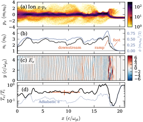
Figure 1: Overview of $\mathcal{M}_{\mathrm{ms}}=3.1$, $\beta_{\mathrm{p}}=0.25$ shock at $t=1253\;{\omega_{\mathrm{pi}}}^{-1}=14.2\;{\Omega_{\mathrm{i}}}^{-1}$. (a) Ion $x$-$p_{x}$ phase-space distribution for full domain, where $p_{x}$ is ion $x$-momentum normalized to upstream momentum $m_{\mathrm{i}}u_{0}$. (b) Ion density $n_{\mathrm{i}}/n_{0}$ (black) and electromotive force $\phi(x)=-\int_{\infty}^{x}E_{x}(x^{\prime})\mathrm{d}x^{\prime}$ in units of $m_{\mathrm{i}}{u_{\mathrm{sh}}}^{2}/2$ (light blue). Both curves are 1-D volume-weighted averages over $y$. The shock foot, ramp, and downstream are annotated. (c) Electric field $E_{x}$ normalized to upstream motional field $u_{0}B_{0}/c$ with magnetic field lines overlaid. $\bm{B}$ points up; i.e., along $+\hat{\bm{y}}$. (d) $T_{\mathrm{e}}/T_{\mathrm{i}}$, density-weighted $y$ average (black), compared to prediction for fluid adiabatic electron heating defined in text (blue dotted). Orange cross is starred measurement in Fig. 2(a); cross width is measurement region, and cross height is standard deviation over 2-D region delimited by cross width. An animation of this figure in the online journal plots shows time evolution from $t=0$ to $1253\;{\omega_{\mathrm{pi}}}^{-1}$ and demonstrates that the temperature ratio $T_{\mathrm{e}}/T_{\mathrm{i}}$ stabilizes $\mathord{\sim}3\;c/{\omega_{\mathrm{pi}}}$ downstream of the shock ramp.

The grid cell size $\Delta x=\Delta y=0.1{c/\omega_{\mathrm{pe}}}$ and the timestep $\Delta t=0.045{\omega_{\mathrm{pe}}}^{-1}$ so that $c=0.45\Delta x/\Delta t$. Upstream plasma has $16$ particles per cell per species. We smooth the electric current with 32 sweeps of a three-point binomial (“1-2-1”) filter at each timestep (Birdsall & Langdon, 1991, Appendix C). The $N=32$ sweeps approximate a Gaussian filter with standard deviation $\sqrt{N/2}=4$ cells or $0.4c/\omega_{\mathrm{pe}}$. The filter’s half-power cut-off is at wavenumber $k\approx\sqrt{2/N}(\Delta x)^{-1}=2.5\left(c/\omega_{\mathrm{pe}}\right)^{-1}$, which implies 50% damping at wavelengths $\lambda\approx\pi\sqrt{2N}\Delta=2.5\left(c/\omega_{\mathrm{pe}}\right)$. Electron-scale waves may be damped, but we will later show that electron-scale waves mainly scatter rather than heat. We simulated 2-D $\mathcal{M}_{\mathrm{ms}}=3.1$, $\beta_{\mathrm{p}}=0.25$ shocks with $4\times$ larger or smaller sweep number $N$; the ratio $T_{\mathrm{e}}/T_{\mathrm{i}}$ did not change much. We adjust $T_{0}$, $u_{0}$, and $B_{0}$ to control $\mathcal{M}_{\mathrm{ms}}$ and $\beta_{\mathrm{p}}$ while keeping shocked electrons non-relativistic; i.e., post-shock $k_{\mathrm{B}}T_{\mathrm{e}}\lesssim 0.05m_{\mathrm{e}}c^{2}$. The ratio $\tau=\omega_{\mathrm{pe}}/\Omega_{\mathrm{e}}=2.5$–$11$ ($\tau\gg 1$ for solar wind and astrophysical settings). The transverse ($y$) width is $2.9$–$5.8\;c/\omega_{\mathrm{pi}}=720$–$1440$ cells. Simulation durations are $10$–$20\;{\Omega_{\mathrm{i}}}^{-1}=932$–$2736\;{\omega_{\mathrm{pi}}}^{-1}$ so that post-shock $T_{\mathrm{e}}/T_{\mathrm{i}}$ reaches steady state. The temperatures $T_{\mathrm{\{i,e\}}}$, $T_{\mathrm{\{i,e\}}\parallel}$, and $T_{\mathrm{\{i,e\}}\perp}$ are moments of the particle distribution in a $5^{N}$ cell region, where $N\in\{1,2,3\}$ is the domain dimensionality. The co-moving frame boost for moment calculation uses a fluid velocity also averaged over $5^{N}$ cells. All $\parallel$- and $\perp$-subscripted quantities are taken with respect to local $\bm{B}$.

Fig. 1 shows a representative simulation. Ions transmit or reflect at the shock ramp (Fig. 1(a-b)). The shock front is rippled (Fig. 1(c)). A net $E_{x}$ potential exists across the shock, and $E_{x}$ is also modulated by the $\bm{B}$ rippling wavelength (Fig. 1(b-c)). Reflected ions accelerate in the motional field $E_{z}=u_{0}B_{0}/c$ before re-entering the shock (Leroy et al., 1982); this lowers $T_{\mathrm{e}}/T_{\mathrm{i}}$ in the shock foot (Fig. 1(d)). Electrons heat above adiabatic expectation in the shock ramp and settle to $T_{\mathrm{e}}/T_{\mathrm{i}}\approx 0.4$; no appreciable heating occurs after the shock ramp (Fig. 1(d)). The fluid adiabatic prediction in Fig. 1(d) is $T_{\mathrm{e,ad}}/(T_{\mathrm{i}}+T_{\mathrm{e}}-T_{\mathrm{e,ad}})$, using measured $T_{\mathrm{i}}$ and $T_{\mathrm{e}}$ and assuming $T_{\mathrm{e,ad}}=T_{0}[1+2(n/n_{0})^{\Gamma-1}]/3$ with $\Gamma=2$.

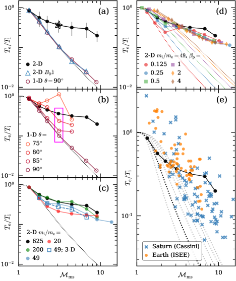
Figure 2: Post-shock $T_{\mathrm{e}}/T_{\mathrm{i}}$ dependence on $\mathcal{M}_{\mathrm{ms}}$ for various setups. All panels: black curve is $T_{\mathrm{e}}/T_{\mathrm{i}}$ from fiducial 2-D $m_{\mathrm{i}}/m_{\mathrm{e}}=625$, $\beta_{\mathrm{p}}=0.25$ shocks. Dotted curves are expected $T_{\mathrm{e}}/T_{\mathrm{i}}$ from MHD shock jump conditions, assuming adiabatic electron heating alone. (a): Varying geometry. 2-D domain with out-of-plane $B_{0}\hat{\bm{z}}$ (triangles) and 1-D domain (hollow circles). Starred datum appears in Figs. 1, 3–4. Error bars on black curve are standard deviation of $T_{\mathrm{e}}/T_{\mathrm{i}}$ within measurement region. (b): 1-D domain, varying $\theta$. Darkest hollow circles ($\theta=90^{\circ}$) same as (a). (c): 2-D domain, varying $m_{\mathrm{i}}/m_{\mathrm{e}}$. Dashed cyan curve with square markers comprises 3-D $m_{\mathrm{i}}/m_{\mathrm{e}}=49$ simulations. (d): 2-D domain, $m_{\mathrm{i}}/m_{\mathrm{e}}=49$, varying $\beta_{\mathrm{p}}$. Dotted curves are adiabatic expectation as in panels (a-c), with $\beta_{\mathrm{p}}$ increasing from left to right. (e): Comparison to solar wind bow shock measurements at Earth (orange circles) (Schwartz et al., 1988) and Saturn (blue crosses) (Masters et al., 2011) as compiled by (Ghavamian et al., 2013). Five Saturn measurements with $\mathcal{M}_{\mathrm{ms}}>20$ are not shown.

3 Shock Parameter Scaling

We measure post-shock $T_{\mathrm{e}}/T_{\mathrm{i}}$ (Fig. 1(c)) as a function of $\mathcal{M}_{\mathrm{ms}}$ for many simulations with varying dimensionality, magnetic field orientation $\theta$, $m_{\mathrm{i}}/m_{\mathrm{e}}$, and $\beta_{\mathrm{p}}$. We also adjust domain width, particle resolution, and current smoothing to control noise and computing cost. In simulations with $\theta<90^{\circ}$, the right-side boundary expands at $\max\left(u_{\mathrm{sh}},0.5c\cos\theta\right)$ to retain shock-reflected electrons streaming along $\bm{B}$.

We show the post-shock $T_{\mathrm{e}}/T_{\mathrm{i}}$ for our fiducial 2-D $m_{\mathrm{i}}/m_{\mathrm{e}}=625$ shocks with in-plane upstream magnetic field $B_{0}\hat{\bm{y}}$ in Fig. 2(a). These fiducial simulations are converged in $T_{\mathrm{e}}/T_{\mathrm{i}}$ with respect to transverse ($y$) width. For perpendicular shocks, we find that electron heating beyond adiabatic compression requires 2-D geometry with in-plane $\bm{B}$. Corresponding 2-D simulations with out-of-plane $\bm{B}$ (along $\hat{\bm{z}}$) and 1-D simulations heat electrons by compression alone (Fig. 2(a)). At $\mathcal{M}_{\mathrm{ms}}\sim 5$–$10$, the 2-D simulations with out-of-plane $\bm{B}$ and 1-D simulations show weak super-adiabatic heating in the shock layer, but the $T_{\mathrm{e}}/T_{\mathrm{i}}$ measurement is also less precise due to numerical heating. Shimada & Hoshino (2000, 2005) saw strong electron heating in 1-D perpendicular $m_{\mathrm{i}}/m_{\mathrm{e}}=20$ shocks due to Buneman instability between shock-reflected ions and incoming electrons. The higher $m_{\mathrm{i}}/m_{\mathrm{e}}=625$ suppresses the Buneman instability in our 1-D shocks.

Can DC heating in a 2-D rippled shock – i.e., varying local magnetic field angle due to self-generated waves – explain the super-adiabatic electron heating seen in our fiducial 2-D simulations? To estimate the DC heating from varying $\theta$, we perform 1-D oblique shock simulations with varying $\theta<90^{\circ}$ (Fig. 2(b)); recall that $\theta$ is the angle between $\bm{B}$ and shock normal. The 1-D setup keeps quasi-static shock structure (averaged over shock reformation cycles) and should retain DC heating while excluding waves oblique to the shock normal. We do find super-adiabatic heating in 1-D oblique shocks. Electrons heat more for lower $\theta$, which is qualitatively consistent with DC field heating (Goodrich & Scudder, 1984). For our representative $\mathcal{M}_{\mathrm{ms}}=3.1$ shock, which has local ripple $\theta\gtrsim 80^{\circ}$ (Fig. 4(f)), the DC heating inferred from 1-D oblique shock simulations appears too low to explain the full amount of super-adiabatic heating (Fig. 2(b, box)).

Our fiducial 2-D perpendicular shocks appear converged in mass ratio at $m_{\mathrm{i}}/m_{\mathrm{e}}\sim 200$–$625$ (Fig. 2(c)), consistent with prior simulations (Umeda et al., 2012a, 2014) and theory (Krauss-Varban et al., 1995). For $m_{\mathrm{i}}/m_{\mathrm{e}}=20$–$625$, 2-D shocks agree on $T_{\mathrm{e}}/T_{\mathrm{i}}$ to within a factor of $2$–$3$. A set of 3-D $m_{\mathrm{i}}/m_{\mathrm{e}}=49$ simulations with narrower transverse width, $2.7c/\omega_{\mathrm{pi}}$, shows good agreement too. Agreement between 2-D and 3-D for $m_{\mathrm{i}}/m_{\mathrm{e}}=49$ suggests that 2-D simulations with in-plane $\bm{B}$ include the essential physics for electron heating.

To see how heating depends on $\beta_{\mathrm{p}}$, we reduce $m_{\mathrm{i}}/m_{\mathrm{e}}$ to $49$ and sweep $\beta_{\mathrm{p}}$ over $0.125$–$4$ (Fig. 2(d)). Electron heating increases above adiabatic at $\mathcal{M}_{\mathrm{ms}}\sim 2$–$3$ for all $\beta_{\mathrm{p}}$. At $\mathcal{M}_{\mathrm{ms}}\sim 3$–$5$ and $\beta_{\mathrm{p}}\leq 1$, two-step $\bm{B}$-parallel electron heating (which we describe below) operates for all $\beta_{\mathrm{p}}\lesssim 1$. At $\mathcal{M}_{\mathrm{ms}}\sim 3$–$5$ and $\beta_{\mathrm{p}}\gtrsim 2$, a distinct electron cyclotron whistler instability is expected to heat electrons instead (Guo et al., 2017, 2018). At $\mathcal{M}_{\mathrm{ms}}\gtrsim 5$, shock structure is more complex, which we do not explore here. The relationship between $T_{\mathrm{e}}/T_{\mathrm{i}}$ and $\mathcal{M}_{\mathrm{ms}}$ does not appear to depend on $\beta_{\mathrm{p}}$ for $\mathcal{M}_{\mathrm{ms}}\gtrsim 4$.

Our fiducial $T_{\mathrm{e}}/T_{\mathrm{i}}$–$\mathcal{M}_{\mathrm{ms}}$ data are order-of-magnitude consistent with measurements from solar wind bow shocks (Fig. 2(e)), replotted from Ghavamian et al. (2013). The Saturn data are uncertain in both $T_{\mathrm{e}}/T_{\mathrm{i}}$ and $\mathcal{M}_{\mathrm{ms}}$ due to a lack of ion temperature measurements from Cassini (Masters et al., 2011), so $\mathcal{M}_{\mathrm{ms}}=0.671\mathcal{M}_{\mathrm{A}}$ (equivalent to $\beta_{\mathrm{p}}\sim 1.5$) is assumed following Ghavamian et al. (2013); we note $\beta_{\mathrm{p}}\sim 1.5$ is a typical value (Richardson, 2002). The Earth data have $\beta_{\mathrm{p}}\sim 0.1$–$1$ and use directly measured ion and electron temperatures from the ISEE spacecraft (Schwartz et al., 1988). Both datasets are mostly quasi-perpendicular, with a majority of shocks having $50^{\circ}<\theta<90^{\circ}$ (Schwartz et al., 1988; Masters et al., 2011).

4 Electron Heating Physics

For further study, we choose the weakest 2-D $m_{\mathrm{i}}/m_{\mathrm{e}}=625$, $\beta_{\mathrm{p}}=0.25$ shock with significant super-adiabatic heating: our representative $\mathcal{M}_{\mathrm{ms}}=3.1$ simulation (Fig. 1, 2(a)). We redo this simulation with higher resolution: $\Delta x=\Delta y=0.05\;{c/\omega_{\mathrm{pe}}}$ (keeping $c=0.45\Delta x/\Delta t$), $64$ particles per cell per species, and $64$ current filter passes per timestep. The current filter approximates a Gaussian with standard deviation $\mathord{\sim}5.7$ cells or $0.28c/\omega_{\mathrm{pe}}$; the filter’s half-power cut-off is at wavenumber $k\approx 3.5\left(c/\omega_{\mathrm{pe}}\right)^{-1}$, which means 50% damping at wavelength $\lambda\approx 1.8c/\omega_{\mathrm{pe}}$. We then select all $15898$ electron particles between $x=8.00$–$8.02\;c/\omega_{\mathrm{pi}}$ at $t^{\prime}\equiv t-324\;{\omega_{\mathrm{pi}}}^{-1}=0$, located $4\;c/\omega_{\mathrm{pi}}=2\;r_{\mathrm{Li}}$ ahead of the shock ramp, and monitor their phase space evolution (Fig. 3) and energy gain (Fig. 4) through the shock. The perpendicular upstream $\bm{B}$ confines particles within a narrow magnetic flux tube and prevents particle drift from downstream to upstream.

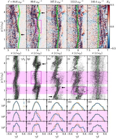
Figure 3: Phase space time evolution (left to right) of electron sample in $\mathcal{M}_{\mathrm{ms}}=3.1$, $\beta_{\mathrm{p}}=0.25$ shock. (a-e): $E_{\parallel}$ normalized to upstream motional field $u_{0}B_{0}/c$ with electron sample overlaid (green dots). Colormap saturates on small-scale waves. (f-j): $\gamma\beta_{\parallel}$–$y$ phase space of electron sample. Green vertical lines mark $\gamma\beta_{\parallel}=0$. (k-o): 1-D $\gamma\beta_{\{\parallel,\perp\}}$ distribution of full electron sample. Thick blue curve is $\gamma\beta_{\parallel}$; orange curve is $\gamma\beta_{\perp}$. (p-t): like (k-o), but only electrons within $y=1.7$–$3.1\;c/\omega_{\mathrm{pi}}$. (u-y): like (k-o), but only electrons within $y=0.6$–$1.4\;c/\omega_{\mathrm{pi}}$. Here $\gamma=1/\sqrt{1-\beta^{2}}$ and $\beta_{\{\parallel,\perp\}}=v_{\{\parallel,\perp\}}/c$. Arrows and boxes discussed in text.

Elongated, ion-scale $E_{\parallel}$ waves accelerate electrons along $\bm{B}$ in the shock foot and ramp. These waves have $|E_{\parallel}|/(u_{0}B_{0}/c)\sim 0.2$–$0.6$ and wavelength $\lambda_{y}\sim 2c/\omega_{\mathrm{pi}}\sim r_{\mathrm{Li}}$ (Fig. 3(a), arrow); we attribute this $E_{\parallel}$ to very oblique whistler waves (i.e., magnetosonic / lower hybrid branch) with fluctuating $E_{x}\gg E_{y},E_{z}$ and $B_{y},B_{z}>B_{x}$, as identified by prior PIC studies (Matsukiyo & Scholer, 2003; Hellinger et al., 2007; Matsukiyo & Scholer, 2006; Umeda et al., 2012b). A stronger bipolar ion-scale $|E_{\parallel}|/(u_{0}B_{0}/c)\gtrsim 0.5$ (Fig. 3(b), arrow) straddles clumps of shock-reflected ions and also accelerates electrons. Accelerated electrons appear as coherent deflections in $\gamma\beta_{\parallel}$–$y$ phase space (Fig. 3(g-h), arrows) that disrupt and relax via two-stream-like instability. Local $y$-regions develop asymmetric and transiently unstable $\gamma\beta_{\parallel}$ distributions (Fig. 3(q,v,x)). Electron relaxation generates strong and rapid electron-scale $E_{\parallel}$ waves and phase-space holes with $\lambda_{y}\sim c/\omega_{\mathrm{pe}}$ (Fig. 3(b,g,i), boxes) (cf. An et al., 2019) Landau damping is evidenced by flattened distributions at $\gamma\beta_{\parallel}\sim 0.2$ (Fig. 3(k-l)). Electrons relax to near isotropy by $t^{\prime}\sim 140\;{\omega_{\mathrm{pi}}}^{-1}$ (Fig. 3(j,o,t,y)). Prior 2-D PIC simulations have shown similar two-step $\bm{B}$-parallel heating in a shock foot setup (periodic interpenetrating beams) (Matsukiyo & Scholer, 2006) and in full shocks (Umeda et al., 2011, 2012b).

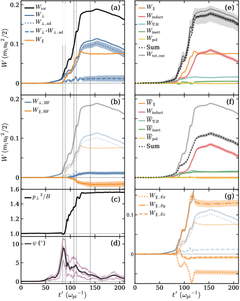
Figure 4: Mean work done on electron sample over time, normalized to upstream ion drift kinetic energy. Vertical dotted lines are snapshot times in Fig. 3. Faded curves in (b,e,f,g) same as (a). Shaded regions are estimated error on coarse-timestep integrated quantities. (a): Decomposition into $W_{\parallel}$, $W_{\perp}$ and adiabatic work $W_{\perp,\mathrm{ad}}$. (b): High-frequency electric field work. (c): Particle-averaged adiabatic moment ${p_{\perp}}^{2}/B$, scaled to mean upstream value. (d): Magnetic field tilt $\psi=\tan^{-1}\left(B_{x}/\sqrt{{B_{y}}^{2}+{B_{z}}^{2}}\right)$ with respect to $y$-$z$ plane. Black curve is particle average $\langle\psi\rangle$; purple curves are 25th, 50th (median), and 75th percentiles. (e): Parallel, induction, $\nabla B$, inertial, and polarization work. Dark-gray region is error for sum of drift work; light-gray region is error for $W_{\mathrm{tot,out}}$. (f): DC-like drift work, defined in text. (g): Parallel work contributions from $E_{x}$, $E_{y}$, and $E_{z}$, as defined in text. The $y$-axis is offset from (a-b,e-f).

$E_{\parallel}$ is the main source of non-adiabatic electron heating (Fig. 4(a)). We decompose the sample electrons’ mean energy gain $W_{\mathrm{tot}}$ into parallel and perpendicular work, $W_{\parallel}=-e\langle\int E_{\parallel}v_{\parallel}\mathrm{d}t\rangle$ and $W_{\perp}=-e\langle\int E_{\perp}v_{\perp}\mathrm{d}t\rangle$, integrated for every particle over every code timestep $\Delta t$ such that $W_{\mathrm{tot}}=W_{\parallel}+W_{\perp}$. Angle brackets are particle averages. We estimate the adiabatic heating as $W_{\perp,\mathrm{ad}}=\langle\sum_{n}(\gamma_{n\to n+1,\mathrm{ad}}-\gamma_{n})m_{\mathrm{e}}c^{2}\rangle$, where

$$\gamma_{n\to n+1,\mathrm{ad}}=\sqrt{1+\left(\gamma\beta_{\parallel}\right)^{2}_{n}+\left(\gamma\beta_{\perp}\right)^{2}_{n}\left(B_{n+1}/B_{n}\right)}$$ (1)

captures electron heating from compression between timesteps $n$ and $n+1$.

In Eqn. (1), we assume $(\gamma\beta_{\perp})^{2}_{n}/B_{n}$ and $(\gamma\beta_{\parallel})_{n}$ are constant during compression; $\gamma$, $\beta_{\parallel}$, and $\beta_{\perp}$ are evaluated in the electron fluid’s rest frame. The sum in $W_{\perp,\mathrm{ad}}$ uses a coarse output timestep $\Delta t_{\mathrm{out}}=400\;\Delta t=9\;{\omega_{\mathrm{pe}}}^{-1}$.

The non-adiabatic perpendicular work can be explained by high-frequency scattering of electron parallel energy into perpendicular energy (Fig. 4(b)). We Fourier-space filter $E_{x}$, $E_{y}$, and $E_{z}$ to isolate wavenumbers $k_{y}>\left(c/\omega_{\mathrm{pe}}\right)^{-1}$ and then construct $E_{\perp,\mathrm{HF}}$ and $E_{\parallel,\mathrm{HF}}$ by projecting the Fourier-filtered fields onto local $\bm{B}$. Then, $W_{\perp,\mathrm{HF}}=-e\langle\sum E_{\perp,\mathrm{HF}}v_{\perp}\Delta t_{\mathrm{out}}\rangle$ and $W_{\parallel,\mathrm{HF}}=-e\langle\sum E_{\parallel,\mathrm{HF}}v_{\parallel}\Delta t_{\mathrm{out}}\rangle$. We find that $W_{\perp,\mathrm{HF}}$ and $W_{\perp}-W_{\perp,\mathrm{ad}}$ agree to $\sim 10\%$, suggesting that non-adiabatic $W_{\perp}$ comes from electron-scale scattering of parallel energy. Exact agreement is not expected due to the coarse timestep $\Delta t_{\mathrm{out}}$ and the arbitrary $k_{y}$ cut.

The particle-averaged adiabatic moment ${p_{\perp}}^{2}/B$ grows in steps that correlate with increases in $W_{\mathrm{tot}}$ and $W_{\parallel}$. Bulk acceleration at $t^{\prime}=84.6\;{\omega_{\mathrm{pi}}}^{-1}$ and $t^{\prime}=107.3\;{\omega_{\mathrm{pi}}}^{-1}$ coincides with momentarily constant ${p_{\perp}}^{2}/B$ and increasing $W_{\parallel}$ prior to a scattering episode. Then, ${p_{\perp}}^{2}/B$ increases during strong electron scattering at $t^{\prime}=89.6\;{\omega_{\mathrm{pi}}}^{-1}$ and $112.3\;{\omega_{\mathrm{pi}}}^{-1}$ while $W_{\parallel}$ flattens off (Fig. 3, Fig. 4(a,c)).

Fig. 4(e) shows mean work from grad B, inertial, and polarization drifts, as well as $\partial B/\partial t$ induction work; see Northrop (1961, 1963); Goodrich & Scudder (1984); Dahlin et al. (2014); Rowan et al. (2019). Each $W_{\mathrm{drift}}=-e\langle\sum\bm{E}\cdot\bm{v}_{\mathrm{drift}}\Delta t_{\mathrm{out}}\rangle$, where $\bm{v}_{\mathrm{drift}}$ is one of:

$$\bm{v}_{\{\nabla B,\mathrm{inert},\mathrm{pol}\}}=-\frac{\gamma m_{\mathrm{e}}c}{eB}\hat{\bm{b}}\times\left\{\frac{{v_{\perp}}^{2}}{2B}\nabla B\bm{,}\,v_{\parallel}\frac{\mathrm{d}\hat{\bm{b}}}{\mathrm{d}t}\bm{,}\,\frac{\mathrm{d}\bm{v}_{E}}{\mathrm{d}t}\right\},$$

with $\gamma$ and $v_{\perp}$ evaluated in the electron fluid’s rest frame. We take $\bm{v}_{E}=\langle c\bm{E}\times\bm{B}/B^{2}\rangle$ to reduce noise; otherwise, the $\bm{v}_{\mathrm{drift}}$ terms use $\bm{E}$ and $\bm{B}$ fields seen by individual particles. The $\mathrm{d}/\mathrm{d}t$ terms are one-sided finite differences; e.g., $\mathrm{d}\bm{v}_{E}/\mathrm{d}t=[(\bm{v}_{E})_{n+1}-(\bm{v}_{E})_{n}]/\Delta t_{\mathrm{out}}$. And, $W_{\mathrm{induct}}=\gamma m_{\mathrm{e}}{v_{\perp}}^{2}(\partial B/\partial t)/(2B)$, with $\partial B/\partial t=[B_{n+1}(\bm{r}_{n})-B_{n-1}(\bm{r}_{n})]/(2\Delta t_{\mathrm{out}})$ and $\bm{r}_{n}$ the particle position at timestep $n$. We find that grad B drift and induction together give fluid-like adiabatic compression. Inertial and polarization drifts give less work, but some other electron samples have $W_{\mathrm{inert}}$ comparable to $W_{\nabla B}$ (Appendix A). We compare the summed drifts to $W_{\mathrm{tot,out}}=-e\langle\sum\bm{E}\cdot\bm{v}\Delta t_{\mathrm{out}}\rangle$. We conclude that $W_{\mathrm{tot}}$ agrees with both the summed drift work and $W_{\mathrm{tot,out}}$, given uncertainty from both the guiding-center drift approximation and the coarse integration timestep.

Earlier, we argued that DC heating alone may not explain all super-adiabatic heating in our fiducial 2-D shock, based on downstream volume-averaged $T_{\mathrm{e}}/T_{\mathrm{i}}$ (Figs. 1(c), 2(b)). So, Fig. 4(f) estimates DC-like work as $\overline{W}_{\mathrm{drift}}=-e\sum\langle\bm{E}\rangle\cdot\langle\bm{v}_{\mathrm{drift}}\rangle\Delta t_{\mathrm{out}}$ and $\overline{W}_{\parallel}=-e\sum\langle E_{\parallel}\rangle\langle v_{\parallel}\rangle\Delta t_{\mathrm{out}}$. The $\bm{E}$ average removes waves along $\hat{\bm{y}}$ to keep only 1-D-like shock fields. The $\bm{v}_{\mathrm{drift}}$ average gives a mean drift trajectory and mostly discards gyration. The DC-like parallel work $\overline{W}_{\parallel}$ goes to zero, and the DC-like contribution to super-adiabatic heating appears small. Fluid-like adiabatic compression is preserved in $W_{\mathrm{induct}}+\overline{W}_{\nabla B}$. Fig. 4(g) separates $E_{x}$, $E_{y}$, and $E_{z}$ contributions to $W_{\parallel}$ as $W_{\parallel,Ei}=-e\langle\sum E_{i}b_{i}v_{\parallel}\Delta t_{\mathrm{out}}\rangle$, where $i=x,y,z$ and $b_{i}$ is the $i$-th component of $\hat{\bm{b}}$. $E_{y}$ gives parallel heating, whereas $E_{x}$ and $E_{z}$ cause parallel cooling.

The quantities $W_{\perp,\mathrm{ad}}$, $W_{\{\parallel,\perp\},\mathrm{HF}}$, $W_{\mathrm{drift}}$, $W_{\mathrm{tot,out}}$, $\overline{W}_{\mathrm{drift}}$, $\overline{W}_{\parallel}$, and $W_{\parallel,Ei}$ are integrated with coarse timestep $\Delta t_{\mathrm{out}}$ and converged at the $\mathord{\sim}10\%$ level. The error regions in Fig. 4(a,b,e) are defined in Appendix B.

5 Conclusion

We have measured $T_{\mathrm{e}}/T_{\mathrm{i}}$ in 2-D PIC simulations of perpendicular shocks to inform models of astrophysical systems lacking direct $T_{\mathrm{e}}$ or $T_{\mathrm{i}}$ measurements. In a $\mathcal{M}_{\mathrm{ms}}=3.1$, $\beta_{\mathrm{p}}=0.25$ rippled shock, quasi-static DC fields provide fluid-like adiabatic heating, and most super-adiabatic heating is from ion-scale $E_{\parallel}$ waves.

Appendix A More Views of Electron Sample Heating

Figs. 5 and 6 present two movies, available online, of our electron sample traversing the shock front.

In Fig. 7, we show the work decomposition from Fig. 4 for many electron samples. At $t^{\prime}=0\;{\omega_{\mathrm{pi}}}^{-1}$, we selected all electrons in the regions $x\in[5.60,5.62]c/\omega_{\mathrm{pi}}$, $x\in[6.00,6.02]c/\omega_{\mathrm{pi}}$, and so on with even spacing $0.4c/\omega_{\mathrm{pi}}$ to get seventeen electron particle samples of similar size.

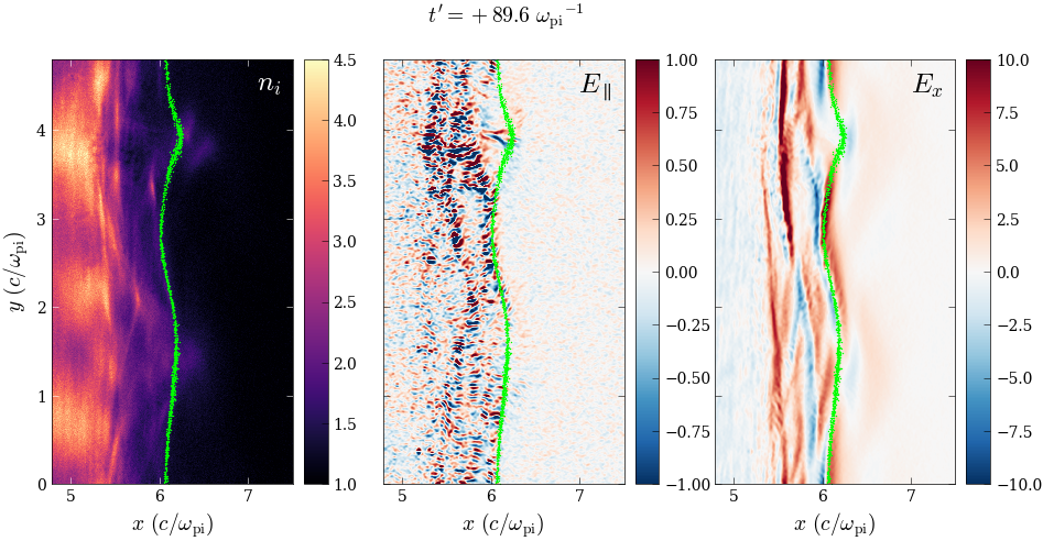
Figure 5: Movie still: electron sample at $t^{\prime}=89.6\;{\omega_{\mathrm{pi}}}^{-1}$ plotted over ion density $n_{\mathrm{i}}$, parallel electric field $E_{\parallel}$, and electric field component $E_{x}$; same sample from Figs. 3 and 4. An animation of this figure from $t^{\prime}=54$ to $180\;{\omega_{\mathrm{pi}}}^{-1}$. is in the online journal. The ion density $n_{\mathrm{i}}$ is scaled to upstream density $n_{0}$, and the electric field components are scaled to upstream motional electric field magnitude $u_{0}B_{0}/c$. The $E_{\parallel}$ colormap spans $[-1,+1]$ and saturates on small-scale waves, despite being a wider range than Fig. 3.

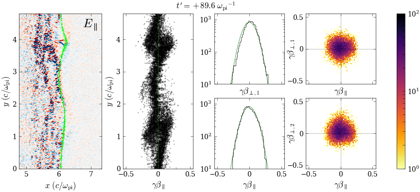
Figure 6: Movie still: electron sample phase space at $t^{\prime}=89.6\;{\omega_{\mathrm{pi}}}^{-1}$, with more detail than Fig. 3. An animation of this figure from $t^{\prime}=54$ to $180\;{\omega_{\mathrm{pi}}}^{-1}$. is in the online journal. The momentum component $\gamma\beta_{\perp,1}$ is the projection along $(\hat{\bm{b}}\times-\hat{\bm{x}})\times\hat{\bm{b}}$, and the component $\gamma\beta_{\perp,2}$ is the projection along $\hat{\bm{b}}\times-\hat{\bm{x}}$. Because the local magnetic field unit vector $\hat{\bm{b}}$ mostly orients along $\hat{\bm{y}}$, the components $\perp,1$ and $\perp,2$ roughly correspond to $-\hat{\bm{x}}$ and $+\hat{\bm{z}}$ so that ($\perp,1$; $\perp,2$; $\parallel$) form a right-handed coordinate system. In the 1-D phase space plots, the light green curve is an isotropic Maxwell-Jüttner distribution with same mean energy as the electrons. The $E_{\parallel}$ colormap is the same as in Fig. 5.

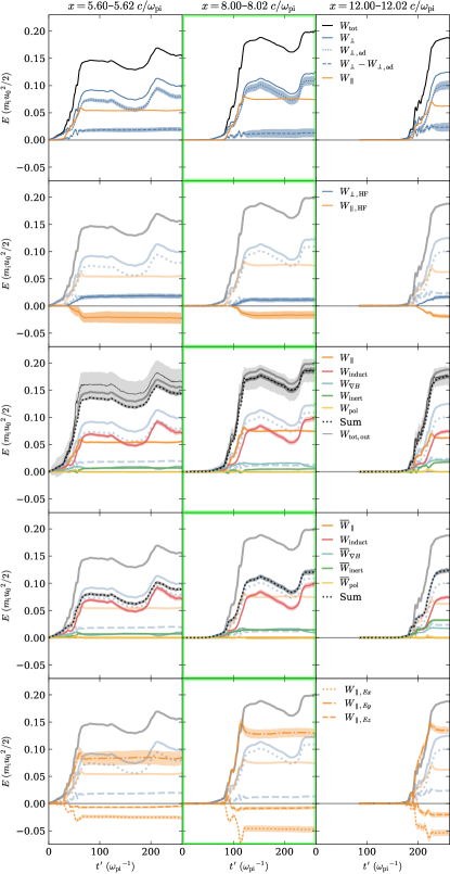
Figure 7: Like Fig. 4(a-b,e-g), but for multiple electron samples traversing the shock at different times. Left and right: first and last samples tracked. Middle (green box): sample shown in Figs. 3 and 4. Column titles indicate the sample’s location at $t^{\prime}=0\;{\omega_{\mathrm{pi}}}^{-1}$. The complete figure (17 samples) is available in the online journal.

Fig. Set7. Electron Work Decomposition

Appendix B Convergence in Electron Work Summation

Several quantities in Figure 4 are summed with a coarse timestep $\Delta t_{\mathrm{out}}=400\Delta t=9\;{\omega_{\mathrm{pe}}}^{-1}$, namely: $W_{\mathrm{\perp,ad}}$, $W_{\mathrm{\perp}}-W_{\mathrm{\perp,ad}}$, $W_{\mathrm{\perp,HF}}$, $W_{\mathrm{\parallel,HF}}$, $W_{\mathrm{induct}}$, $W_{\mathrm{\nabla B}}$, $W_{\mathrm{inert}}$, $W_{\mathrm{pol}}$, $W_{\mathrm{tot,out}}$, $\overline{W}_{\mathrm{\nabla B}}$, $\overline{W}_{\mathrm{inert}}$, $\overline{W}_{\mathrm{pol}}$, $\overline{W}_{\parallel}$, $W_{\parallel,Ex}$, $W_{\parallel,Ey}$, and $W_{\parallel,Ez}$. To check convergence, we downsample in time each quantity’s summand by $4$ and compute an error $\delta f$ at discrete time $t_{n}$ as:

$$\delta f(t_{n})=\max\left\{\left|f(t_{m})-f_{1/4}(t_{m})\right|\mid 0\leq m\leq n\right\}$$ (B1)

where $f_{1/4}$ is the $4\times$ downsampled version of $f$. Thus $\delta f$ is strictly non-decreasing with $t_{n}$. The error regions defined by Eq. B1 are plotted as shaded areas in Figs. 4 and 7.

Fig. 8 shows curves with $2,4,8\times$ downsampling for the seventeen distinct electron samples of Fig. 7, including the sample shown in Fig. 4.

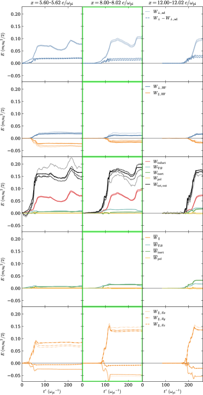
Figure 8: Like Fig. 7, but showing the numerical convergence of all quantities integrated with the coarse timestep $\Delta t_{\mathrm{out}}$, listed in text. For each quantity, we increase the sample spacing $\Delta t_{\mathrm{out}}$ by $2\times$, $4\times$, and $8\times$ and plot the down-sampled integration with progressively decreasing opacity. The complete figure (17 samples) is available in the online journal.

Fig. Set8. Electron Work Convergence

Appendix C Transverse Width Convergence

Fig. 9 shows that our fiducial 2-D simulations are converged with respect to transverse width. Most of the varying transverse width simulations are not listed in Table D. For $\mathcal{M}_{\mathrm{ms}}=9.1$ only, the 1-D simulation uses a slightly higher upstream temperature than the 2-D simulations, so the ratio $\Omega_{\mathrm{i}}/\omega_{\mathrm{pi}}$ differs between 1-D and 2-D. In this case, we matched times based on ${\Omega_{\mathrm{i}}}^{-1}$ rather than ${\omega_{\mathrm{pi}}}^{-1}$.

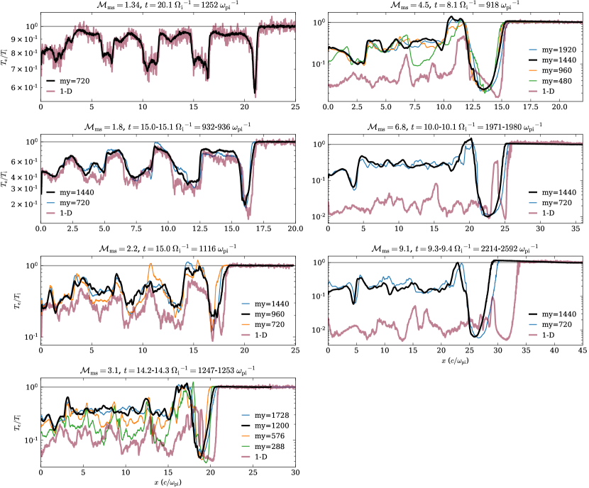
Figure 9: Fiducial 2-D simulations are converged with respect to transverse width. Black curves are fiducial 2-D $m_{\mathrm{i}}/m_{\mathrm{e}}=625$, $\beta_{\mathrm{p}}=0.25$ simulations from Fig. 2(a). Colored curves are same shock parameters with varying input my, as defined in Table D. A time range is given because simulation output times do not match exactly.

Appendix D Simulation Parameters

Table D contains input parameters, derived shock parameters, run durations, and downstream temperature measurements for all simulations in our manuscript. The first row is the high-resolution run used in Figs. 3 and 4; the remaining rows are presented in Fig. 2. A machine-readable version of Table D, in comma-separated value (CSV) ASCII, is available in the online journal. Below, we define all table columns.

• mi_me is the ion-electron mass ratio $m_{\mathrm{i}}/m_{\mathrm{e}}$.

• theta and phi specify the upstream magnetic field orientation, measured in the simulation frame. $\theta$ is the angle between $\bm{B}$ and the $x$-coordinate axis. $\varphi$ is the angle between the $y$-$z$ plane projection of $\bm{B}$ and the $z$-coordinate axis. To visualize these angles, see Fig. 1 of Guo et al. (2014), but note that their $\varphi_{\mathrm{B}}=\pi/2-\varphi$ is the complement of our $\varphi$. For all our simulations, $\theta$ corresponds to the angle between $\bm{B}$ and shock normal. The 2-D simulations with in-plane $\bm{B}$ have $\theta=90^{\circ}$ and $\varphi=90^{\circ}$. The 2-D simulations with out-of-plane $\bm{B}$ (i.e., $\bm{B}$ along $\hat{\bm{z}}$) have $\theta=90^{\circ}$ and $\varphi=0^{\circ}$. The 1-D simulations with oblique $\bm{B}$ have have $\theta<90^{\circ}$.

• my and mz are the numbers of grid cells along $\hat{\bm{y}}$ and $\hat{\bm{z}}$. Our 2-D simulations have $\mathtt{mz}=1$, and 1-D simulations have $\mathtt{my}=\mathtt{mz}=1$.

• betap, Ms, Ma, and Mms are the shock plasma beta $\beta_{\mathrm{p}}$, sonic Mach number $\mathcal{M}_{\mathrm{s}}$, Alfvén Mach number $\mathcal{M}_{\mathrm{A}}$, and fast magnetosonic Mach number $\mathcal{M}_{\mathrm{ms}}$. These numbers are derived from TRISTAN-MP input parameters sigma, delgam, and u0 (defined just below). First, the total plasma beta is:

  $$\beta_{\mathrm{p}}=\frac{4\gamma_{0}\Delta\gamma_{\mathrm{i}}}{\sigma\left(\gamma_{0}-1\right)\left(1+m_{\mathrm{e}}/m_{\mathrm{i}}\right)}$$

  where $\gamma_{0}=1/\sqrt{1-\left(u_{0}/c\right)^{2}}$ is the Lorentz factor of the upstream flow in the simulation frame. The sonic Mach number depends on the upstream plasma speed in the shock’s rest frame:

  $$\mathcal{M}_{\mathrm{s}}=\frac{u_{\mathrm{sh}}}{c_{\mathrm{s}}}=\frac{u_{\mathrm{0}}}{\left(1-1/r\left(\mathcal{M}_{\mathrm{s}}\right)\right)c_{\mathrm{s}}}$$

  and we solve this implicit expression for $\mathcal{M}_{\mathrm{s}}$ (and thus also $u_{\mathrm{sh}}$) using an input $u_{\mathrm{0}}$ and assumed fluid adiabatic index $\Gamma=2$ (note that $\Gamma$ enters into both the Rankine-Hugoniot expression for MHD shock compression ratio $r$ and the sound speed $c_{\mathrm{s}}$). Once $\mathcal{M}_{\mathrm{s}}$ and $u_{\mathrm{sh}}$ are known, $\mathcal{M}_{\mathrm{A}}$ and $\mathcal{M}_{\mathrm{ms}}$ are known as well. This procedure for estimating shock parameters is taken directly from Guo et al. (2017).

• sigma is the magnetization, a ratio of upstream magnetic and kinetic enthalpy densities:

  $$\texttt{sigma}=\sigma\equiv\frac{{B_{0}}^{2}}{4\pi\left(\gamma_{0}-1\right)\left(m_{\mathrm{i}}+m_{\mathrm{e}}\right)n_{0}c^{2}}.$$

• delgam is the upstream plasma temperature, scaled by ion rest energy:

  $$\texttt{delgam}=\Delta\gamma_{\mathrm{i}}\equiv\frac{k_{\mathrm{B}}T_{0}}{m_{\mathrm{i}}c^{2}}.$$

• u0 is the upstream plasma velocity, scaled by speed of light:

  $$\texttt{u0}\equiv u_{0}/c$$

• ppc0 is number of particles (both electrons and ions) per cell in the upstream plasma.

• c_omp is the number of grid cells per electron skin depth $c/\omega_{\mathrm{pe}}$.

• ntimes is the number of current filter passes.

• dur is the simulation duration in units of upstream ion cyclotron time ${\Omega_{\mathrm{i}}}^{-1}$.

• Te_Ti is our measurement of downstream temperature ratio $T_{\mathrm{e}}/T_{\mathrm{i}}$. As described in the main text, we manually choose a downstream region that is minimally affected by the left-side reflecting wall and the right-side shock front relaxation. Our measurement of $T_{\mathrm{e}}/T_{\mathrm{i}}$ uses downsampled grid output of the particle temperature tensor; however, the temperature tensor itself is calculated for each grid cell using the full particle distribution in a $5^{N}$ cell region, where $N\in\{1,2,3\}$ is the domain dimensionality.

• Te_Ti_std is the standard deviation of $T_{\mathrm{e}}/T_{\mathrm{i}}$ within the downstream region that we consider. Like Te_Ti, downsampled grid output is used for this estimate.

• Te and Ti are the downstream electron and ion temperatures scaled to their respective rest masses; i.e., $k_{\mathrm{B}}T_{\mathrm{e}}/(m_{\mathrm{e}}c^{2})$ and $k_{\mathrm{B}}T_{\mathrm{i}}/(m_{\mathrm{i}}c^{2})$. We measure all of Te, Ti, and Te_Ti in the same manually-chosen downstream region.

=0.2in mi_me theta phi my mz betap Ms Ma Mms sigma delgam u0 ppc0 c_omp ntimes dur Te_Ti Te_Ti_std Te Ti 625 90 90 2400 1 0.250 6.86 3.43 3.07 4.7854E$-$1 8.0944E$-$6 2.3245E$-$2 128 20 64 6.7  $\cdots$  $\cdots$  $\cdots$  $\cdots$ 625 90 90 720 1 0.251 3.00 1.50 1.34 1.0117E$+$1 1.6189E$-$5 7.1502E$-$3 32 10 32 20.1 8.53E$-$1 1.38E$-$1 1.29E$-$2 2.43E$-$5 625 90 90 1440 1 0.250 4.00 2.00 1.79 2.3774E$+$0 1.6189E$-$5 1.4749E$-$2 32 10 32 15.0 5.59E$-$1 2.33E$-$1 1.74E$-$2 4.96E$-$5 625 90 90 960 1 0.250 5.00 2.50 2.24 1.1237E$+$0 1.1332E$-$5 1.7949E$-$2 32 10 32 20.1 4.52E$-$1 1.69E$-$1 1.96E$-$2 6.92E$-$5 625 90 90 1200 1 0.250 6.86 3.43 3.07 4.7854E$-$1 8.0944E$-$6 2.3245E$-$2 32 10 32 14.2 3.65E$-$1 1.28E$-$1 2.83E$-$2 1.24E$-$4 625 90 90 1440 1 0.250 9.99 4.99 4.47 1.9968E$-$1 4.8566E$-$6 2.7873E$-$2 32 10 32 12.1 3.18E$-$1 1.22E$-$1 3.65E$-$2 1.83E$-$4 625 90 90 1440 1 0.250 15.19 7.60 6.79 8.1402E$-$2 1.6189E$-$6 2.5205E$-$2 32 10 32 10.0 2.97E$-$1 1.22E$-$1 2.80E$-$2 1.51E$-$4 625 90 90 1440 1 0.250 20.37 10.18 9.11 4.4398E$-$2 8.0944E$-$7 2.4133E$-$2 32 10 32 9.8 1.98E$-$1 5.99E$-$2 1.83E$-$2 1.47E$-$4 625 90 0 1440 1 0.251 3.00 1.50 1.34 1.0117E$+$1 1.6189E$-$5 7.1502E$-$3 32 10 32 19.0 8.62E$-$1 1.20E$-$1 1.30E$-$2 2.42E$-$5 625 90 0 1440 1 0.250 4.00 2.00 1.79 2.3774E$+$0 1.6189E$-$5 1.4749E$-$2 32 10 32 19.9 4.71E$-$1 1.78E$-$1 1.60E$-$2 5.42E$-$5 625 90 0 1440 1 0.250 5.00 2.50 2.24 1.1237E$+$0 1.1332E$-$5 1.7949E$-$2 32 10 32 15.0 2.49E$-$1 1.28E$-$1 1.24E$-$2 7.93E$-$5 625 90 0 1440 1 0.250 7.00 3.50 3.13 4.5493E$-$1 8.0944E$-$6 2.3840E$-$2 32 10 32 15.2 1.07E$-$1 5.45E$-$2 1.02E$-$2 1.54E$-$4 625 90 0 1440 1 0.250 10.00 5.00 4.47 1.9912E$-$1 4.8566E$-$6 2.7912E$-$2 32 10 32 9.8 4.48E$-$2 2.30E$-$2 6.82E$-$3 2.44E$-$4 625 90 0 1440 1 0.250 15.00 7.50 6.71 8.3580E$-$2 1.6189E$-$6 2.4874E$-$2 32 10 32 8.5 2.54E$-$2 2.43E$-$2 3.11E$-$3 1.96E$-$4 625 90 90 1 1 0.251 3.00 1.50 1.34 1.0117E$+$1 1.6189E$-$5 7.1502E$-$3 512 10 32 40.0 8.52E$-$1 1.05E$-$1 1.32E$-$2 2.47E$-$5 625 90 90 1 1 0.250 4.00 2.00 1.79 2.3774E$+$0 1.6189E$-$5 1.4749E$-$2 512 10 32 40.0 4.28E$-$1 1.86E$-$1 1.58E$-$2 5.92E$-$5 625 90 90 1 1 0.250 5.00 2.50 2.24 1.1237E$+$0 1.1332E$-$5 1.7949E$-$2 512 10 32 25.2 2.36E$-$1 8.40E$-$2 1.24E$-$2 8.40E$-$5 625 90 90 1 1 0.250 7.00 3.50 3.13 4.5493E$-$1 8.0944E$-$6 2.3840E$-$2 512 10 32 25.0 1.01E$-$1 3.87E$-$2 1.02E$-$2 1.61E$-$4 625 90 90 1 1 0.250 10.00 5.00 4.47 1.9912E$-$1 4.8566E$-$6 2.7912E$-$2 512 10 32 15.2 5.02E$-$2 3.44E$-$2 7.03E$-$3 2.24E$-$4 625 90 90 1 1 0.250 15.00 7.50 6.71 8.3580E$-$2 1.6189E$-$6 2.4874E$-$2 1024 10 32 15.1 2.38E$-$2 1.57E$-$2 2.85E$-$3 1.92E$-$4 625 90 90 1 1 0.250 20.00 10.00 8.94 4.6080E$-$2 1.1332E$-$6 2.8027E$-$2 2048 10 32 10.1 1.35E$-$2 1.18E$-$2 2.05E$-$3 2.43E$-$4 625 85 90 1 1 0.251 3.00 1.50 1.34 1.0117E$+$1 1.6189E$-$5 7.1502E$-$3 2048 10 64 40.0 9.15E$-$1 7.96E$-$2 1.36E$-$2 2.38E$-$5 625 85 90 1 1 0.250 4.00 2.00 1.79 2.3774E$+$0 1.6189E$-$5 1.4749E$-$2 2048 10 64 40.0 4.91E$-$1 1.61E$-$1 1.70E$-$2 5.54E$-$5 625 85 90 1 1 0.250 5.00 2.50 2.23 1.1237E$+$0 1.1332E$-$5 1.7949E$-$2 2048 10 64 25.2 2.79E$-$1 1.57E$-$1 1.36E$-$2 7.79E$-$5 625 85 90 1 1 0.250 7.00 3.50 3.13 4.5493E$-$1 8.0944E$-$6 2.3840E$-$2 2048 10 64 20.0 1.35E$-$1 4.98E$-$2 1.35E$-$2 1.60E$-$4 625 85 90 1 1 0.250 10.00 5.00 4.47 1.9912E$-$1 4.8566E$-$6 2.7912E$-$2 2048 10 64 15.2 1.29E$-$1 3.69E$-$2 1.75E$-$2 2.17E$-$4 625 80 90 1 1 0.251 2.99 1.50 1.34 1.0117E$+$1 1.6189E$-$5 7.1502E$-$3 2048 10 64 30.1 8.73E$-$1 4.51E$-$2 1.27E$-$2 2.32E$-$5 625 80 90 1 1 0.250 3.99 2.00 1.79 2.3774E$+$0 1.6189E$-$5 1.4749E$-$2 2048 10 64 30.1 6.58E$-$1 1.09E$-$1 1.94E$-$2 4.72E$-$5 625 80 90 1 1 0.250 4.99 2.50 2.23 1.1237E$+$0 1.1332E$-$5 1.7949E$-$2 2048 10 64 25.2 5.28E$-$1 1.62E$-$1 2.13E$-$2 6.45E$-$5 625 80 90 1 1 0.250 6.99 3.49 3.13 4.5493E$-$1 8.0944E$-$6 2.3840E$-$2 2048 10 64 20.0 2.38E$-$1 1.27E$-$1 2.05E$-$2 1.38E$-$4 625 80 90 1 1 0.250 9.99 5.00 4.47 1.9912E$-$1 4.8566E$-$6 2.7912E$-$2 2048 10 64 15.2 1.89E$-$1 8.87E$-$2 2.27E$-$2 1.91E$-$4 625 75 90 1 1 0.251 2.98 1.49 1.34 1.0117E$+$1 1.6189E$-$5 7.1502E$-$3 2048 10 64 40.0 8.54E$-$1 2.44E$-$2 1.27E$-$2 2.37E$-$5 625 75 90 1 1 0.250 3.98 1.99 1.78 2.3774E$+$0 1.6189E$-$5 1.4749E$-$2 2048 10 64 30.1 6.45E$-$1 7.82E$-$2 1.94E$-$2 4.80E$-$5 625 75 90 1 1 0.250 4.98 2.49 2.23 1.1237E$+$0 1.1332E$-$5 1.7949E$-$2 2048 10 64 25.2 7.76E$-$1 1.81E$-$1 2.69E$-$2 5.55E$-$5 625 75 90 1 1 0.250 6.98 3.49 3.12 4.5493E$-$1 8.0944E$-$6 2.3840E$-$2 2048 10 64 20.0 1.11E$+$0 1.90E$-$1 5.52E$-$2 7.95E$-$5 625 75 90 1 1 0.250 9.98 4.99 4.46 1.9912E$-$1 4.8566E$-$6 2.7912E$-$2 2048 10 64 15.2 2.58E$-$1 1.27E$-$1 3.09E$-$2 1.92E$-$4 20 90 90 720 1 0.250 3.00 1.50 1.34 9.8755E$+$0 5.0590E$-$4 3.9505E$-$2 32 10 32 39.2 8.62E$-$1 9.55E$-$2 1.29E$-$2 7.46E$-$4 20 90 90 720 1 0.250 4.00 2.00 1.79 2.2975E$+$0 5.0590E$-$4 8.1851E$-$2 32 10 32 39.2 4.43E$-$1 1.69E$-$1 1.58E$-$2 1.79E$-$3 20 90 90 720 1 0.250 5.00 2.50 2.24 1.0872E$+$0 3.5413E$-$4 9.9512E$-$2 32 10 32 29.5 2.83E$-$1 1.40E$-$1 1.38E$-$2 2.44E$-$3 20 90 90 720 1 0.250 6.84 3.42 3.06 4.6363E$-$1 2.5295E$-$4 1.2868E$-$1 32 10 32 24.5 2.13E$-$1 8.37E$-$2 1.73E$-$2 4.07E$-$3 20 90 90 720 1 0.250 9.93 4.97 4.44 1.9289E$-$1 1.5177E$-$4 1.5439E$-$1 32 10 32 19.6 1.85E$-$1 8.66E$-$2 2.34E$-$2 6.33E$-$3 20 90 90 720 1 0.250 15.12 7.56 6.76 7.9463E$-$2 5.0590E$-$5 1.3896E$-$1 32 10 32 14.7 1.70E$-$1 4.14E$-$2 1.82E$-$2 5.36E$-$3 20 90 90 960 1 0.250 20.27 10.14 9.07 4.3483E$-$2 2.5295E$-$5 1.3285E$-$1 32 10 32 14.7 1.64E$-$1 4.36E$-$2 1.69E$-$2 5.15E$-$3 49 90 90 1440 1 0.250 3.00 1.50 1.34 1.0020E$+$1 2.0649E$-$4 2.5420E$-$2 32 10 32 39.5 8.53E$-$1 1.09E$-$1 1.28E$-$2 3.07E$-$4 49 90 90 1440 1 0.250 4.00 2.00 1.79 2.3453E$+$0 2.0649E$-$4 5.2528E$-$2 32 10 32 39.5 4.78E$-$1 2.11E$-$1 1.59E$-$2 6.78E$-$4 49 90 90 1440 1 0.250 5.00 2.50 2.24 1.1090E$+$0 1.4454E$-$4 6.3899E$-$2 32 10 32 25.0 3.37E$-$1 1.71E$-$1 1.54E$-$2 9.32E$-$4 49 90 90 1440 1 0.250 6.85 3.42 3.06 4.7256E$-$1 1.0325E$-$4 8.2703E$-$2 32 10 32 25.6 3.26E$-$1 1.43E$-$1 2.35E$-$2 1.47E$-$3 49 90 90 1440 1 0.250 9.97 4.98 4.46 1.9696E$-$1 6.1947E$-$5 9.9192E$-$2 32 10 32 25.0 2.75E$-$1 6.97E$-$2 3.22E$-$2 2.39E$-$3 49 90 90 720 1 0.250 15.16 7.58 6.78 8.0625E$-$2 2.0649E$-$5 8.9530E$-$2 128 10 32 15.0 1.81E$-$1 4.46E$-$2 1.92E$-$2 2.16E$-$3 49 90 90 720 1 0.250 20.33 10.17 9.09 4.4032E$-$2 1.0325E$-$5 8.5672E$-$2 128 10 32 14.9 1.32E$-$1 3.76E$-$2 1.42E$-$2 2.19E$-$3 49 90 90 360 1 0.250 30.63 15.32 13.70 1.9157E$-$2 4.1298E$-$6 8.2153E$-$2 128 10 32 10.0 1.14E$-$1 3.67E$-$2 1.11E$-$2 1.97E$-$3 200 90 90 1440 1 0.250 3.00 1.50 1.34 1.0099E$+$1 5.0590E$-$5 1.2629E$-$2 32 10 32 33.1 8.54E$-$1 1.16E$-$1 1.28E$-$2 7.49E$-$5 200 90 90 1440 1 0.250 4.00 2.00 1.79 2.3715E$+$0 5.0590E$-$5 2.6060E$-$2 32 10 32 39.3 5.40E$-$1 2.04E$-$1 1.80E$-$2 1.66E$-$4 200 90 90 1440 1 0.250 5.00 2.50 2.24 1.1210E$+$0 3.5413E$-$5 3.1711E$-$2 32 10 32 29.0 4.75E$-$1 2.00E$-$1 2.03E$-$2 2.14E$-$4 200 90 90 1440 1 0.250 6.86 3.43 3.07 4.7744E$-$1 2.5295E$-$5 4.1064E$-$2 32 10 32 21.5 3.66E$-$1 1.52E$-$1 2.67E$-$2 3.65E$-$4 200 90 90 1440 1 0.250 9.98 4.99 4.46 1.9918E$-$1 1.5177E$-$5 4.9241E$-$2 32 10 32 20.0 3.73E$-$1 1.16E$-$1 3.91E$-$2 5.24E$-$4 200 90 90 1440 1 0.250 15.18 7.59 6.79 8.1259E$-$2 5.0590E$-$6 4.4512E$-$2 32 10 32 15.0 2.44E$-$1 7.44E$-$2 2.51E$-$2 5.14E$-$4 200 90 90 1440 1 0.250 20.36 10.18 9.11 4.4331E$-$2 2.5295E$-$6 4.2614E$-$2 64 10 32 10.2 1.51E$-$1 6.25E$-$2 1.55E$-$2 5.13E$-$4 49 90 90 192 192 0.250 4.00 2.00 1.79 2.3453E$+$0 2.0649E$-$4 5.2528E$-$2 32 10 32 24.1 4.65E$-$1 2.23E$-$1 1.57E$-$2 6.90E$-$4 49 90 90 192 192 0.250 5.00 2.50 2.24 1.1090E$+$0 1.4454E$-$4 6.3899E$-$2 32 10 32 35.3 3.37E$-$1 2.07E$-$1 1.57E$-$2 9.54E$-$4 49 90 90 192 384 0.250 6.85 3.42 3.06 4.7256E$-$1 1.0325E$-$4 8.2703E$-$2 32 10 32 17.4 2.74E$-$1 1.40E$-$1 2.12E$-$2 1.58E$-$3 49 90 90 192 192 0.250 9.97 4.98 4.46 1.9696E$-$1 6.1947E$-$5 9.9192E$-$2 32 10 32 15.0 2.37E$-$1 1.61E$-$1 2.84E$-$2 2.45E$-$3 49 90 90 192 192 0.250 15.16 7.58 6.78 8.0625E$-$2 2.0649E$-$5 8.9530E$-$2 32 10 32 8.9 1.50E$-$1 7.62E$-$2 1.58E$-$2 2.16E$-$3 49 90 90 1440 1 0.125 4.00 1.41 1.33 1.1537E$+$1 2.0649E$-$4 3.3500E$-$2 32 10 32 24.8 7.71E$-$1 1.32E$-$1 1.28E$-$2 3.38E$-$4 49 90 90 1440 1 0.125 5.00 1.77 1.67 3.4565E$+$0 1.4454E$-$4 5.1197E$-$2 32 10 32 24.8 4.14E$-$1 1.98E$-$1 1.06E$-$2 5.22E$-$4 49 90 90 1440 1 0.125 6.68 2.36 2.23 1.2431E$+$0 1.0325E$-$4 7.2128E$-$2 32 10 32 25.0 2.42E$-$1 1.35E$-$1 1.14E$-$2 9.66E$-$4 49 90 90 1440 1 0.125 9.78 3.46 3.26 4.4927E$-$1 6.1947E$-$5 9.2894E$-$2 32 10 32 24.8 3.09E$-$1 1.34E$-$1 2.68E$-$2 1.77E$-$3 49 90 90 1440 1 0.125 14.99 5.30 5.00 1.7122E$-$1 2.0649E$-$5 8.6888E$-$2 32 10 32 20.1 2.65E$-$1 8.51E$-$2 2.32E$-$2 1.79E$-$3 49 90 90 1440 1 0.125 20.19 7.14 6.73 9.1148E$-$2 1.0325E$-$5 8.4213E$-$2 32 10 32 15.1 2.10E$-$1 6.01E$-$2 1.88E$-$2 1.83E$-$3 49 90 90 360 1 0.125 30.53 10.79 10.18 3.8916E$-$2 4.1298E$-$6 8.1516E$-$2 128 10 32 10.1 1.47E$-$1 8.28E$-$2 1.36E$-$2 1.89E$-$3 49 90 90 720 1 0.500 2.00 1.41 1.15 3.5805E$+$1 2.0649E$-$4 9.5092E$-$3 32 10 32 38.8 9.95E$-$1 6.62E$-$2 1.14E$-$2 2.34E$-$4 49 90 90 1440 1 0.500 3.00 2.12 1.73 2.2310E$+$0 2.0649E$-$4 3.8088E$-$2 32 10 32 38.8 6.17E$-$1 1.70E$-$1 1.54E$-$2 5.09E$-$4 49 90 90 1440 1 0.500 3.87 2.74 2.24 9.2639E$-$1 2.0649E$-$4 5.9093E$-$2 32 10 32 25.9 3.99E$-$1 1.41E$-$1 1.93E$-$2 9.85E$-$4 49 90 90 1440 1 0.500 4.90 3.47 2.83 4.8236E$-$1 1.4454E$-$4 6.8506E$-$2 32 10 32 26.0 4.00E$-$1 1.29E$-$1 2.30E$-$2 1.17E$-$3 49 90 90 1440 1 0.500 6.98 4.93 4.03 2.0639E$-$1 1.0325E$-$4 8.8477E$-$2 32 10 32 25.6 2.80E$-$1 5.22E$-$2 2.81E$-$2 2.04E$-$3 49 90 90 1440 1 0.500 10.08 7.13 5.82 9.2084E$-$2 6.1947E$-$5 1.0257E$-$1 32 10 32 25.5 2.05E$-$1 3.55E$-$2 2.94E$-$2 2.94E$-$3 49 90 90 1440 1 0.500 15.26 10.79 8.81 3.9095E$-$2 2.0649E$-$5 9.0910E$-$2 32 10 32 19.9 1.47E$-$1 1.99E$-$2 1.78E$-$2 2.47E$-$3 49 90 90 1440 1 1.000 2.00 2.00 1.41 4.4802E$+$0 2.0649E$-$4 1.9008E$-$2 32 10 32 25.0 9.19E$-$1 1.39E$-$1 1.34E$-$2 2.97E$-$4 49 90 90 1440 1 1.000 3.00 3.00 2.12 8.2034E$-$1 2.0649E$-$4 4.4412E$-$2 32 10 32 25.0 5.18E$-$1 1.55E$-$1 1.76E$-$2 6.95E$-$4 49 90 90 1440 1 1.000 4.00 4.00 2.83 3.6299E$-$1 2.0649E$-$4 6.6745E$-$2 32 10 32 25.0 3.64E$-$1 1.08E$-$1 2.37E$-$2 1.33E$-$3 49 90 90 1440 1 1.000 4.99 4.99 3.53 2.1083E$-$1 1.4454E$-$4 7.3265E$-$2 32 10 32 24.8 3.42E$-$1 8.28E$-$2 2.55E$-$2 1.52E$-$3 49 90 90 1440 1 1.000 7.06 7.06 4.99 9.6333E$-$2 1.0325E$-$4 9.1569E$-$2 32 10 32 24.8 2.18E$-$1 3.84E$-$2 2.54E$-$2 2.37E$-$3 49 90 90 1440 1 1.000 10.15 10.15 7.18 4.4490E$-$2 6.1947E$-$5 1.0434E$-$1 32 10 32 25.0 1.59E$-$1 2.53E$-$2 2.49E$-$2 3.19E$-$3 49 90 90 1440 1 1.000 15.31 15.31 10.82 1.9246E$-$2 2.0649E$-$5 9.1619E$-$2 32 10 32 24.8 1.32E$-$1 1.91E$-$2 1.64E$-$2 2.53E$-$3 49 90 90 1440 1 2.000 2.00 2.83 1.63 1.4344E$+$0 2.0649E$-$4 2.3754E$-$2 32 10 32 24.8 8.56E$-$1 1.86E$-$1 1.50E$-$2 3.58E$-$4 49 90 90 1440 1 2.000 3.00 4.24 2.45 3.5747E$-$1 2.0649E$-$4 4.7572E$-$2 32 10 32 24.8 5.24E$-$1 9.73E$-$2 2.04E$-$2 7.93E$-$4 49 90 90 1512 1 2.000 4.00 5.66 3.27 1.6927E$-$1 2.0649E$-$4 6.9110E$-$2 32 10 32 27.8 3.39E$-$1 4.34E$-$2 2.63E$-$2 1.59E$-$3 49 90 90 1512 1 2.000 5.00 7.07 4.08 1.0012E$-$1 2.0649E$-$4 8.9824E$-$2 32 10 32 24.6 2.58E$-$1 3.86E$-$2 3.21E$-$2 2.55E$-$3 49 90 90 1440 1 2.000 7.11 10.05 5.80 4.6506E$-$2 1.0325E$-$4 9.3186E$-$2 32 10 32 24.9 1.86E$-$1 2.32E$-$2 2.42E$-$2 2.66E$-$3 49 90 90 2016 1 2.000 10.19 14.41 8.32 2.1861E$-$2 6.1947E$-$5 1.0525E$-$1 32 10 32 18.8 1.33E$-$1 1.29E$-$2 2.26E$-$2 3.46E$-$3 49 90 90 1440 1 2.000 15.33 21.69 12.52 9.5477E$-$3 2.0649E$-$5 9.1978E$-$2 32 10 32 12.0 1.22E$-$1 2.36E$-$2 1.57E$-$2 2.63E$-$3 49 90 90 1440 1 4.000 2.00 4.00 1.79 5.9285E$-$1 2.0649E$-$4 2.6126E$-$2 32 10 32 25.1 8.35E$-$1 1.87E$-$1 1.62E$-$2 3.96E$-$4 49 90 90 1512 1 4.000 3.00 6.00 2.68 1.6743E$-$1 2.0649E$-$4 4.9151E$-$2 32 10 32 23.8 4.90E$-$1 6.76E$-$2 2.21E$-$2 9.19E$-$4 49 90 90 1512 1 4.000 4.00 8.00 3.58 8.1810E$-$2 2.0649E$-$4 7.0292E$-$2 32 10 32 34.3 3.45E$-$1 4.17E$-$2 2.79E$-$2 1.65E$-$3 49 90 90 1512 1 4.000 5.00 10.00 4.47 4.9023E$-$2 2.0649E$-$4 9.0767E$-$2 32 10 32 36.6 2.60E$-$1 2.30E$-$2 3.32E$-$2 2.61E$-$3 49 90 90 1440 1 4.000 7.13 14.27 6.38 2.2843E$-$2 1.0325E$-$4 9.4017E$-$2 32 10 32 25.1 1.69E$-$1 1.46E$-$2 2.31E$-$2 2.79E$-$3 49 90 90 2160 1 4.000 10.21 20.42 9.13 1.0835E$-$2 6.1947E$-$5 1.0571E$-$1 32 10 32 19.0 1.35E$-$1 1.22E$-$2 2.33E$-$2 3.52E$-$3

Table 1: Simulation input parameters, derived shock parameters, run duration, and downstream temperature measurements. Columns are defined in Appendix D.

Note. — Table D is available in a machine-readable CSV format in the online journal.

References

- An et al. (2019) An, X., Li, J., Bortnik, J., et al. 2019, Phys. Rev. Lett., 122, 045101
- Avestruz et al. (2015) Avestruz, C., Nagai, D., Lau, E. T., & Nelson, K. 2015, ApJ, 808, 176
- Birdsall & Langdon (1991) Birdsall, C. K., & Langdon, A. B. 1991, Plasma Physics via Computer Simulation, The Adam Hilger Series on Plasma Physics (Bristol, England: IOP Publishing Ltd)
- Buneman (1993) Buneman, O. 1993, in Computer Space Plasma Physics: Simulation Techniques and Software, ed. H. Matsumoto & Y. Omura (Tokyo: Terra Scientific), 67–84
- Chen et al. (2018) Chen, L.-J., Wang, S., Wilson, III, L. B., et al. 2018, Physical Review Letters, 120, 225101
- Cohen et al. (2019) Cohen, I. J., Schwartz, S. J., Goodrich, K. A., et al. 2019, Journal of Geophysical Research (Space Physics), 124, 3961
- Dahlin et al. (2014) Dahlin, J. T., Drake, J. F., & Swisdak, M. 2014, Physics of Plasmas, 21, 092304
- Dimmock et al. (2019) Dimmock, A. P., Russell, C. T., Sagdeev, R. Z., et al. 2019, Science Advances, 5, eaau9926
- Feldman et al. (1982) Feldman, W. C., Bame, S. J., Gary, S. P., et al. 1982, Physical Review Letters, 49, 199
- Feldman et al. (1983) Feldman, W. C., Anderson, R. C., Bame, S. J., et al. 1983, J. Geophys. Res., 88, 96
- Ghavamian et al. (2013) Ghavamian, P., Schwartz, S. J., Mitchell, J., Masters, A., & Laming, J. M. 2013, Space Sci. Rev., 178, 633
- Goodrich & Scudder (1984) Goodrich, C. C., & Scudder, J. D. 1984, J. Geophys. Res., 89, 6654
- Goodrich et al. (2018) Goodrich, K. A., Ergun, R., Schwartz, S. J., et al. 2018, Journal of Geophysical Research (Space Physics), 123, 9430
- Guo et al. (2014) Guo, X., Sironi, L., & Narayan, R. 2014, ApJ, 794, 153
- Guo et al. (2017) —. 2017, ApJ, 851, 134
- Guo et al. (2018) —. 2018, ApJ, 858, 95
- Hanson et al. (2019) Hanson, E. L. M., Agapitov, O. V., Mozer, F. S., et al. 2019, Geophys. Res. Lett., 46, 2381
- Helder et al. (2010) Helder, E. A., Kosenko, D., & Vink, J. 2010, ApJ, 719, L140
- Hellinger et al. (2007) Hellinger, P., Trávníček, P., Lembège, B., & Savoini, P. 2007, Geophys. Res. Lett., 34, L14109
- Hovey et al. (2018) Hovey, L., Hughes, J. P., McCully, C., Pandya, V., & Eriksen, K. 2018, ApJ, 862, 148
- Hull et al. (2001) Hull, A. J., Scudder, J. D., Larson, D. E., & Lin, R. 2001, J. Geophys. Res., 106, 15711
- Johlander et al. (2016) Johlander, A., Schwartz, S. J., Vaivads, A., et al. 2016, Phys. Rev. Lett., 117, 165101
- Krasnoselskikh et al. (2002) Krasnoselskikh, V. V., Lembège, B., Savoini, P., & Lobzin, V. V. 2002, Physics of Plasmas, 9, 1192
- Krauss-Varban et al. (1995) Krauss-Varban, D., Pantellini, F. G. E., & Burgess, D. 1995, Geophys. Res. Lett., 22, 2091
- Lefebvre et al. (2007) Lefebvre, B., Schwartz, S. J., Fazakerley, A. F., & Décréau, P. 2007, Journal of Geophysical Research (Space Physics), 112, A09212
- Leroy et al. (1982) Leroy, M. M., Winske, D., Goodrich, C. C., Wu, C. S., & Papadopoulos, K. 1982, J. Geophys. Res., 87, 5081
- Lowe & Burgess (2003) Lowe, R. E., & Burgess, D. 2003, Annales Geophysicae, 21, 671
- Masters et al. (2011) Masters, A., Schwartz, S. J., Henley, E. M., et al. 2011, Journal of Geophysical Research (Space Physics), 116, A10107
- Matsukiyo & Scholer (2003) Matsukiyo, S., & Scholer, M. 2003, Journal of Geophysical Research (Space Physics), 108, 1459
- Matsukiyo & Scholer (2006) —. 2006, Journal of Geophysical Research (Space Physics), 111, A06104
- Muschietti & Lembège (2017) Muschietti, L., & Lembège, B. 2017, Annales Geophysicae, 35, 1093
- Northrop (1961) Northrop, T. G. 1961, Annals of Physics, 15, 79
- Northrop (1963) —. 1963, Reviews of Geophysics and Space Physics, 1, 283
- Richardson (2002) Richardson, J. D. 2002, Planet. Space Sci., 50, 503
- Rowan et al. (2019) Rowan, M. E., Sironi, L., & Narayan, R. 2019, ApJ, 873, 2
- Schwartz (2014) Schwartz, S. J. 2014, Journal of Geophysical Research (Space Physics), 119, 1507
- Schwartz et al. (1988) Schwartz, S. J., Thomsen, M. F., Bame, S. J., & Stansberry, J. 1988, J. Geophys. Res., 93, 12923
- Scudder (1996) Scudder, J. D. 1996, J. Geophys. Res., 101, 2561
- Scudder et al. (1986) Scudder, J. D., Mangeney, A., Lacombe, C., et al. 1986, J. Geophys. Res., 91, 11075
- Shimada & Hoshino (2000) Shimada, N., & Hoshino, M. 2000, ApJ, 543, L67
- Shimada & Hoshino (2005) —. 2005, Journal of Geophysical Research (Space Physics), 110, A02105
- Sironi & Spitkovsky (2009) Sironi, L., & Spitkovsky, A. 2009, ApJ, 698, 1523
- Spitkovsky (2005) Spitkovsky, A. 2005, in AIP Conference Proceedings, Vol. 801, Astrophysical Sources of High Energy Particles and Radiation, ed. T. Bulik, B. Rudak, & G. Madejski (Melville, New York: American Institute of Physics), 345–350
- Umeda et al. (2012a) Umeda, T., Kidani, Y., Matsukiyo, S., & Yamazaki, R. 2012a, Physics of Plasmas, 19, 042109
- Umeda et al. (2012b) —. 2012b, Journal of Geophysical Research (Space Physics), 117, A03206
- Umeda et al. (2014) —. 2014, Physics of Plasmas, 21, 022102
- Umeda et al. (2011) Umeda, T., Yamao, M., & Yamazaki, R. 2011, Planet. Space Sci., 59, 449
- Wilson et al. (2009) Wilson, L. B., I., Cattell, C. A., Kellogg, P. J., et al. 2009, Journal of Geophysical Research (Space Physics), 114, A10106
- Wilson et al. (2014a) Wilson, L. B., Sibeck, D. G., Breneman, A. W., et al. 2014a, Journal of Geophysical Research (Space Physics), 119, 6455
- Wilson et al. (2014b) —. 2014b, Journal of Geophysical Research (Space Physics), 119, 6475
- Wilson et al. (2012) Wilson, III, L. B., Koval, A., Szabo, A., et al. 2012, Geophys. Res. Lett., 39, L08109
- Wu et al. (1984) Wu, C. S., Winske, D., Zhou, Y. M., et al. 1984, Space Sci. Rev., 37, 63
- Yamaguchi et al. (2014) Yamaguchi, H., Eriksen, K. A., Badenes, C., et al. 2014, ApJ, 780, 136