A panoramic landscape of the Sagittarius stream in Gaia DR2
revealed with the STREAMFINDER spyglass

Abstract

We present the first full six-dimensional panoramic portrait of the Sagittarius stream, obtained by searching for wide stellar streams in the Gaia DR2 dataset with the STREAMFINDER algorithm. We use the kinematic behavior of the sample to devise a selection of Gaia RR Lyrae, providing excellent distance measurements along the stream. The proper motion data are complemented with radial velocities from public surveys. We find that the global morphological and kinematic properties of the Sagittarius stream are still reasonably well reproduced by the simple Law & Majewski (2010) model (LM10), although the model overestimates the leading arm and trailing arm distances by up to $\sim 15$%. The sample newly reveals the leading arm of the Sagittarius stream as it passes into very crowded regions of the Galactic disk towards the Galactic Anticenter direction. Fortuitously, this part of the stream is almost exactly at the diametrically opposite location from the Galactic Center to the progenitor, which should allow an assessment of the influence of dynamical friction and self-gravity in a way that is nearly independent of the underlying Galactic potential model.

1 Introduction

The Sagittarius dwarf galaxy (Ibata et al., 1994) is one the major contributors to the stellar populations of the Galactic halo (Newberg et al., 2002; Belokurov et al., 2006). It is currently $\sim 19{\rm\,kpc}$ behind the Galactic bulge, and dissolving rapidly under the influence of the strong tides at that location. The tidally-disrupted stars that have been removed from the progenitor now form a vast, almost polar band, that wraps more than a full revolution around the sky (Ibata et al., 2001; Majewski et al., 2003). It has long been appreciated that this system can inform us about the processes of minor mergers and satellite accretion, and the fundamental problem of the distribution of dark matter, both in the Milky Way and in its satellites.

Early simulations attempted to understand how such an apparently fragile system could survive to be seen at the present time, concluding that some dark matter component in the dwarf was probably necessary (Ibata & Lewis, 1998). The structure and kinematics of the stream indicated that the Galactic potential was roughly spheroidal, although different analyses concluded that the most likely shape was either spherical (Ibata et al., 2001), slightly oblate (Law et al., 2005) or slightly prolate (Helmi, 2004), apparently dependent on the location of the tracers employed.

A subsequent in-depth analysis (Law & Majewski, 2010, hereafter LM10) of an all-sky survey of M-giant stars, found that a triaxial Galactic potential model could resolve these conflicts. The proposed model had the surprising property of being significantly flattened along the Sun-Galactic center axis, which is difficult to reconcile with the dynamics of a stable disk configuration (Debattista et al., 2013). Nevertheless, this model has held up remarkably well to subsequent observations of the Sagittarius system, and despite its limitations (Law & Majewski, 2016) it has become the reference against which other models are held up (see, e.g., Thomas et al., 2017; Fardal et al., 2019).

Here we revisit this structure, using the superb new data from Second Data Release (DR2) of the Gaia mission (Lindegren et al., 2018; Gaia Collaboration et al., 2018). Our approach will be to use the STREAMFINDER algorithm (Malhan & Ibata, 2018; Malhan et al., 2018) to identify stars that have a high likelihood of belonging to physically wide streams, such as that of the Sagittarius dwarf. Our aim is to provide the community with an effective means to select high-probability members of the stream from Gaia data.

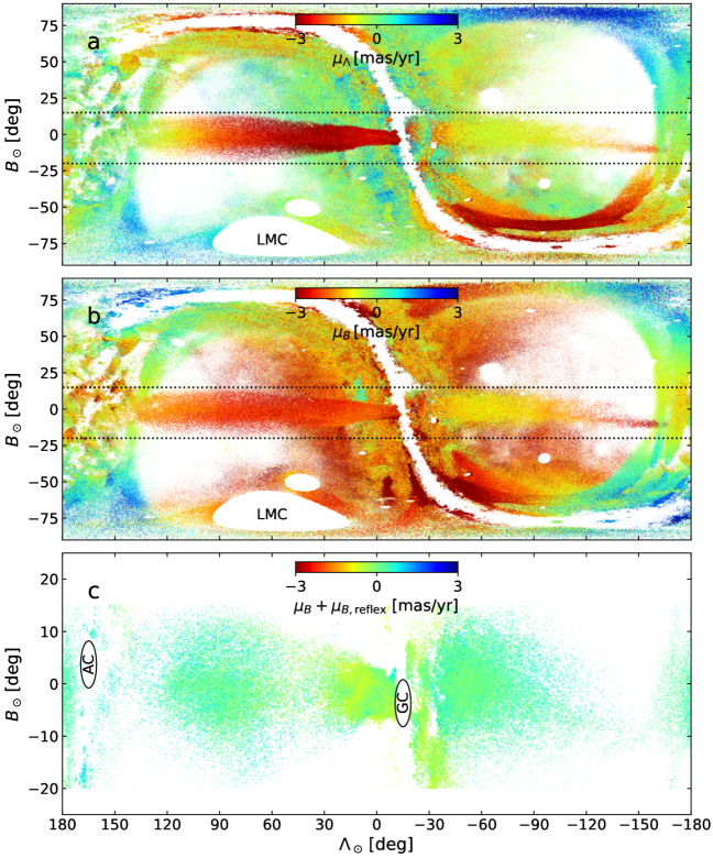
Figure 1: Maps of STREAMFINDER detections with stream significance $>15\sigma$ using a stream template of Gaussian width $0.5{\rm\,kpc}$ and a stellar populations template of age $12.5{\rm\,Gyr}$ and metallicity ${\rm[Fe/H]=-1.1}$. The $\Lambda_{\odot},B_{\odot}$ Sagittarius coordinates shown are aligned such that $\Lambda_{\odot}$ points along the stream and $B_{\odot}$ is orthogonal to $\Lambda_{\odot}$. The proper motions in those directions, $\mu_{\Lambda}$ and $\mu_{B}$, are displayed on the top and middle panels. Panel c shows the $\mu_{B}$ proper motion corrected for Solar reflex motion for the final cleaned sample of 263,438 stars. Galactic satellites (e.g., the LMC) were masked-out in the input catalog. The positions of the Galactic Center and Galactic Anticenter are marked ’GC’ and ’AC’, respectively.

2 STREAMFINDER selection

We re-analysed the Gaia DR2 dataset with the STREAMFINDER algorithm in an almost identical way to the procedure described in Ibata et al. (2019, hereafter IMM19). As in IMM19, we only considered stars down to a limiting magnitude of $G_{0}=19.5$ (fainter sources were discarded to minimise spatial inhomogeneities in the maps). Magnitudes were corrected for extinction using the Schlegel et al. (1998) maps, adopting the re-calibration by Schlafly & Finkbeiner (2011), with $R_{V}=3.1$. The full sky was processed, although circular regions surrounding known satellites (but not the Sagittarius dwarf galaxy) were ignored. This masking of satellites is explained in detail in IMM19.

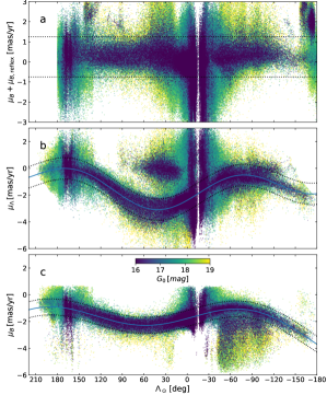
Figure 2: Cleaning of the sample. After limiting the sources to $-20^{\circ}<B<15^{\circ}$, as shown in Figure 1, we limit the sample to $-0.75<\mu_{B}+\mu_{B,\rm reflex}<1.25{\rm\,mas/yr}$ (panel a). This constrains the stars to move along the orbit. b: The sample is trimmed further, taking $|\mu_{\Lambda}-\mu_{\Lambda,\rm fit}|<0.8{\rm\,mas/yr}$. c: Finally, we take $|\mu_{B}-\mu_{B,\rm fit}|<0.6{\rm\,mas/yr}$. The color of the points encode the $G_{0}$-band magnitude of the stars, and are shown here because the astrometric uncertainties are primarily a function of $G$.

The STREAMFINDER is effectively a friend-finding algorithm that considers each star in a dataset in turn, and searches for similar stars in a tube along all the possible orbits of the star under consideration (the orbits are integrated in the potential model #1 of Dehnen & Binney 1998). The algorithm requires a stream template model as input. In the present work we adopted a stream width of (Gaussian) dispersion $0.5{\rm\,kpc}$, and allowed the algorithm to search for friends along a $20^{\circ}$-long orbit. We ran the process with three different stellar populations templates from the PARSEC library (Bressan et al., 2012) of age and metallicity $(T,{\rm[Fe/H]})$: $(8{\rm\,Gyr},-1.4)$, $(12.5{\rm\,Gyr},-1.1)$, $(12.5{\rm\,Gyr},-1.7)$. Here we present the results using the $(12.5{\rm\,Gyr},-1.1)$ model, which gave the best match to the RR Lyrae distances calculated below. However, the samples derived from the three age-metallicity templates choices yield essentially identical proper motion profiles. The algorithm was only allowed to search for distance solutions in the Heliocentric range $d_{\odot}=[10,100]{\rm\,kpc}$. All other parameters were the same as in IMM19. These include using a Galactcentric distance of $R_{\odot}=8.122\pm 0.031{\rm\,kpc}$ (Gravity Collaboration et al., 2018), and adopting a circular velocity of $v_{c}(R_{\odot})=229.0\pm 0.2{\rm\,km\,s^{-1}}$ (Eilers et al., 2019). Given that $v_{c}(R_{\odot})+V_{\rm LSR,\,pec}+V_{\odot}=255.2\pm 5.1{\rm\,km\,s^{-1}}$ (Reid et al., 2014), we take the sum of the $V$-component of the peculiar velocity of the Sun and $V$-component of the peculiar velocity of the Local Standard of Rest to be $V_{\odot}+V_{\rm LSR,\,pec}=26.2{\rm\,km\,s^{-1}}$, while the $U$ and $W$ components of the Sun’s peculiar velocity are taken from Schönrich et al. (2010).

Figure 1 shows the resulting map of the stars in Gaia DR2 that exhibit stream-like behavior with significance $>15\sigma$. The $\Lambda_{\odot},B_{\odot}$ coordinate system used is a version of the Heliocentric Sagittarius coordinates devised by Majewski et al. (2003), although here we follow the choice of Koposov et al. (2012) of inverting $B_{\odot}$ (so the maps are more easily compared to standard maps made in equatorial coordinates). The pole of the Great Circle is at $(\ell,b)=(273\hbox{${}^{\circ}$\hskip-3.0pt.}8,-13\hbox{${}^{\circ}$\hskip-3.0pt.}5)$, with zero-point of $\Lambda_{\odot}$ at the position of the globular cluster M54, commonly accepted to be the center of the system (Bellazzini et al., 2008). The most recently-disrupted stars in the leading arm have negative values of $\Lambda_{\odot}$, and the dwarf galaxy is moving towards negative $\Lambda_{\odot}$. In panels (a) and (b) we display $\mu_{\Lambda}$ and $\mu_{B}$, respectively, which are the Gaia proper motion measurements rotated into these Sagittarius coordinates. The Sagittarius stream stands out as one of the most striking features in this all-sky map. It spans the entire sky and, as shown by Belokurov et al. (2006) and Koposov et al. (2012), it is bifurcated into two parallel arms over much of its length. Its varying width is a projection effect due to the large range of heliocentric distance it covers. Other known streams are present, and some potential new streams appear to have been detected, but we defer their analysis to a subsequent contribution. Visual inspection shows that the Sagittarius stream is present in the range $B=[-20^{\circ},15^{\circ}]$ (between the dotted lines in Figure 1), and henceforth we consider only those (755,343) stars that lie within this band.

While internally the STREAMFINDER constructs associations between stars in a catalog, it proved to be impractical for computer memory reasons to store these links. Some post-processing is therefore required to disentangle the Sagittarius stream from other stream-like features. The adopted selection procedure is described in Figure 2.

The stars in a stream will generally not have large motions in the direction perpendicular to the orbit, unless there are strong perturbers (see, e.g. Erkal et al. 2019). For this reason, in Figure 2a we conservatively take the broad selection in $-0.75{\rm\,mas/yr}<\mu_{B}+\mu_{B,\rm reflex}<1.25{\rm\,mas/yr}$ of the proper perpendicular to the Sagittarius plane (corrected for the reflex motion $\mu_{B,\rm reflex}$ of the Sun in the direction of $B_{\odot}$). To compute $\mu_{B,\rm reflex}$, we assume the Galactic geometry and Solar motion described in IMM19, and use the distance to the stars that is estimated by the STREAMFINDER software. The sample is clearly displaced with respect to the expected $\mu_{B}+\mu_{B,\rm reflex}=0{\rm\,mas/yr}$ line; the reason for this is unclear, but it may indicate that the stellar distances are underestimated (by $\sim 10$%), or that the adopted model of the Solar motion is imprecise. This selection leaves 539,707 stars.

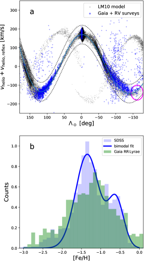
Figure 3: a: Radial velocities of the cleaned STREAMFINDER sample, as measured in public spectroscopic surveys. The behavior of the younger tidal arms in the ($<3{\rm\,Gyr}$) LM10 model are also shown, along with a sinusoidal fit to these particles (solid line). The magenta circle highlights the nearby leading arm. b: The metallicity distribution of the SDSS-Segue stars (blue) in the sample (and that also lie between the dotted lines in panel a) is compared to the Gaia RR Lyrae sample (green). The blue line shows a bimodal Gaussian fit to the Segue sample.

In Figure 2b, we show the subsequent selection on $\mu_{\Lambda}$. To model the sinusoidal behavior of the stream we fit a model to the brighter stars with $G_{0}<17.5$ using an iterative sigma-clipping procedure. The displayed model has the form:

$$\mu_{\Lambda,\rm fit}(\Lambda_{\odot})=a_{1}\sin(a_{2}\Lambda_{\odot}+a_{3})+a_{4}+a_{5}\Lambda_{\odot}+a_{6}\Lambda_{\odot}^{2}$$ (1)

and the best-fitting parameters (with $\Lambda_{\odot}$ in degrees) were found to be: $a_{1}=1.1842$, $a_{2}=-1.5639\times\pi/180$, $a_{3}=-0.39917$, $a_{4}=-1.9307$, $a_{5}=-8.0606\times 10^{-4}$ and $a_{6}=3.2441\times 10^{-5}$. The 331,795 stars with $|\mu_{\Lambda}-\mu_{\Lambda,\rm fit}|<0.8{\rm\,mas/yr}$ (a $2\sigma$ limit) were retained.

We also make a selection on $\mu_{B}$, as shown in Figure  2c. The fitted function, $\mu_{B,\rm fit}(\Lambda_{\odot})$ has the same functional form as $\mu_{\Lambda,\rm fit}(\Lambda_{\odot})$, but with parameters $a_{1}=-1.2360$, $a_{2}=1.0910\times\pi/180$, $a_{3}=0.36330$, $a_{4}=-1.3412$, $a_{5}=7.3022\times 10^{-3}$ and $a_{6}=-4.3315\times 10^{-5}$. By selecting $|\mu_{B}-\mu_{B,\rm fit}|<0.6{\rm\,mas/yr}$ (again a $2\sigma$ limit), we obtain a final sample of 263,438 candidate stream stars. The spatial distribution of these sources is displayed in Figure 1c, and they are listed in Table 1.

We cross-matched these sources with public spectroscopic surveys, and found 2984 matches (212 in APOGEE, Majewski et al. 2017; 35 in the Gaia Radial Velocity Spectrometer sample; 1236 in LAMOST, Cui et al. 2012; 1 in RAVE, Kunder et al. 2017; and 1500 in SDSS-Segue, Yanny et al. 2009). The radial velocities of these stars are shown in Figure 3a along with the LM10 simulation. The improvement in terms of contamination in this STREAMFINDER sample over large pre-Gaia surveys can be appreciated by comparing Figure 3a to the SDSS study by Gibbons et al. (2017) (their Figure 1). The sub-sample with radial velocities can be used as a control sample to estimate the contamination fraction. To this end, we fit a sinusoid to the young ($<3{\rm\,Gyr}$) arms of the Sagittarius stream in the LM10 model (blue line), and assume that stars beyond $50{\rm\,km\,s^{-1}}$ (dotted lines) of this fit are Galactic field star contaminants. Given the velocity dispersion of metal-poor stars in the stream ($13{\rm\,km\,s^{-1}}$, Gibbons et al. 2017), this corresponds to a $\sim 4\sigma$ limit, that is wide enough to allow for some model mismatch. The resulting contamination fraction is 18%. Note however, that this is a global value, averaged over the very complex footprint and complex target selection functions of the public radial velocity surveys listed above. Breaking down this test sample by magnitude, we find a contamination fraction of 14% for $G_{0}<17$ mag; of 19% for $G_{0}$ in the range $[17,18]$ mag, and of $30\%$ for $G_{0}>18$ mag. Clearly, the contamination fraction will be dependent on the density of the contaminating populations, and so will be highest at low Galactic latitude. In Figure 1c, the off-track population with $B_{\odot}<-10^{\circ}$ and $\Lambda_{\odot}$ in the range $[-40^{\circ},-20^{\circ}]$ (and which straddles the Galactic plane behind the bulge) looks suspiciously like such contamination.

It is very difficult to predict the effect that the false positives may have on subsequent kinematic analyses, but given that the contamination fraction is relatively small the effect may be small also. Selecting stars closer to the fitted proper motion track helps to reduce the contamination. Taking $|\mu_{\Lambda}-\mu_{\Lambda,\rm fit}|<0.4{\rm\,mas/yr}$ and $|\mu_{B}-\mu_{B,\rm fit}|<0.3{\rm\,mas/yr}$ (i.e. tightening the previous constraints by a factor of 2), yields a sample of 138,165 stars with a contamination fraction of 11%, and estimated in the same way as above).

Considering the sub-sample of stars possessing SDSS radial velocity and metallicity measurements, we find $\langle{\rm[Fe/H]}\rangle=-1.24$ dex ($-1.40$ dex) and $\sigma_{\rm[Fe/H]}=0.52$ dex ($0.60$ dex) for the velocity-confirmed members (non-members). The similarity of the metallicity distributions of the stream and the contaminants means that metallicity can only be weakly correlated with the contamination probability. Furthermore, the correlation between $B_{\odot}$ and ${\rm[Fe/H]}$ is very low, with a Spearman’s rank coefficient of $\rho=0.004$, and $\rho=-0.024$ for the correlation between $|B_{\odot}|$ and ${\rm[Fe/H]}$. This confirms that the populations of different metallicities are not appreciably displaced perpendicular to the stream track (and shows again that metallicity cannot be a primary driver of contamination probability).

One might be concerned that the stellar populations template used in the STREAMFINDER could introduce a strong bias against stars of different metallicity. This is not the case, as we show in Figure 3b, where we display the metallicity distribution of the sample with SDSS-Segue metallicities and that are confirmed velocity members (blue). Fitting a bimodal Gaussian to these data (blue line) yields means of ${\rm[Fe/H]}=-1.35$ and ${\rm[Fe/H]}=-0.61$ with metallicity dispersions of $0.30$ dex and $0.20$ dex, respectively. These values are extremely close to the trailing arm fit by Gibbons et al. (2017): ${\rm[Fe/H]}=-1.33$ and ${\rm[Fe/H]}=-0.74$ with dispersions $0.27$ dex and $0.18$ dex, respectively. Thus the STREAMFINDER sample does not have an obvious metallicity bias.

The Gaia DR2 catalog is known to have a small $0.029$ mas parallax bias (Lindegren et al., 2018). Assuming that the correlation matrix of the astrometric solution is valid in the context of this small parallax bias, we can use the Gaia parallax_pmra_corr and parallax_pmdec_corr terms to derive the resulting proper motion bias. The resulting mean bias values for the present sample are $-0.005{\rm\,mas/yr}$ (rms scatter $0.007{\rm\,mas/yr}$) and $0.002{\rm\,mas/yr}$ (rms scatter $0.006{\rm\,mas/yr}$) for the bias in $\mu_{\alpha}$ and $\mu_{\delta}$, respectively. If there are any applications of this dataset that need a mean accuracy beyond this level, they will need to update the proper motion values in Table 1 using the Early Data Release 3 catalog (expected for late 2020).

In a recent analysis of the GD-1 stellar stream, we showed that a sample derived with the STREAMFINDER software had a statistically-identical density profile to samples defined in a more traditional way by sigma-clipping, followed by background subtraction (Ibata et al., 2020). Thus, at least for mono-metallicity populations, the algorithm does not produce samples with peculiar completeness properties. However, in the present work, we cleaned the initial STREAMFINDER sample with the three proper motion filters depicted in Figure 2 in order to better isolate the Sagittarius stream stars and reduce the number of false positives. Unfortunately, the proper motion uncertainties of fainter stars will cause genuine members to drop out of the selection windows (we note that the most stringent cut of $0.6{\rm\,mas/yr}$ on $|\mu_{B}-\mu_{B,\rm fit}|$ corresponds to the typical proper motion uncertainty at $G_{0}\sim 19$ mag). This will lead to an increasing incompleteness of the faint stars. Studies that require sample completeness will need to correct for this loss of members. We estimate the incompleteness caused by these three proper motion filters by applying them to a version of the LM10 model where the N-body particles are assigned a $G$-band magnitude drawn from the PARSEC model with $(T,{\rm[Fe/H]})=(12.5{\rm\,Gyr},-1.1)$. Only the particles within $180^{\circ}$ of the progenitor are considered (i.e. we neglect older wraps). Proper motion uncertainties are assigned as a function of $G$ using the median values listed in Lindegren et al. (2018), and the model proper motions are degraded accordingly. We thereby find that the global incompleteness caused by the three proper motion filters is $<5$% to $G=17.5$ mag, but degrades to $7$% for $G=[17.5,18.5]$ mag, and to $40$% for $G=[18.5,19.5]$ mag.

3 Sagittarius stream RR Lyrae stars in Gaia

The spatial and proper motion selection procedure described above also provides a means to construct a cleaned catalog of Sagittarius RR Lyrae stars, which can serve as distance anchors to the stream. For this we used the RR Lyrae variables identified in the gaiadr2.vari_rrlyrae catalog (Clementini et al., 2019), that is part of Gaia DR2. The catalog includes 140,784 RR Lyrae and provides a metallicity estimate from Fourier parameters of the light curves (see, e.g., Nemec et al. 2013) for 64,932 of them. From this source we selected the subset of 135,825 stars having full 5-parameter astrometric solution. Interstellar extinction was corrected for in the same manner as described above for the main Gaia catalog. After applying the selection on $B_{\odot}$, as well as the proper motion selections presented in Figure 2, we obtain a cleaned sample of (exactly) 3,500 Sagittarius RR Lyrae stars.

For the subset of stars for which metallicity estimates are available in the catalog (1,474 stars), we calculate the distance from the $M_{G}$ – ${\rm[Fe/H]}$ relation by Muraveva et al. (2018). The metallicity distribution of this RR Lyrae sample is displayed in Figure 3b (green); a large metallicity spread is present, but this is also seen in the SDSS-Segue STREAMFINDER sample (blue). The mean metallicity of the RR Lyrae is ${\rm[Fe/H]=-1.3}$, corresponding to $M_{G}=+0.69$, which we adopted for all the RR Lyrae in the sample lacking metallicity. To provide a quantitative idea of the size of the systematic error possibly associated with this choice, the adoption of $M_{G}=0.64$, following Iorio & Belokurov (2019), would lead to a distance scale larger than ours by $2.5$%, a negligible amount in the present context. In Figure 4c we show (in green) the distances to the stream derived from RR Lyrae identified in Pan-STARRS (Hernitschek et al., 2017, hereafter H17). The slight differences as a function of position may be due to the fact that the Gaia RR Lyrae sample is much less contaminated and that the metallicity correction applied here — but which H17 could not implement due to a lack of metallicity information — improves the distances.

The $x$–$z$ plane positions of these stars are compared to the values calculated by the STREAMFINDER in Figure 4a; the good match shows that the STREAMFINDER provides useful estimates of the distance to the Sagittarius stream with the adopted stellar population template.

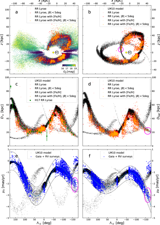
Figure 4: a: The $x$-$z$ plane positions of the cleaned STREAMFINDER sample (colored by their $G_{0}$ magnitude) are compared to the Gaia RR Lyrae stars. Note the good match both to the RR Lyrae stars with metallicity measurements (orange) and without (red). Larger dots mark the stars with $|B|<5^{\circ}$ that better delineate the stream. b: The position of the RR Lyrae are compared to the LM10 model, showing some significant systematic discrepancies both in the leading and trailing arms. The magenta circle highlights the nearby portion of the leading stream seen towards the Galactic Anticenter. (The position of the Sun is marked with a yellow circle, and the Galactic Center is encircled in black). c: Profile in Heliocentric distance. d: Profile in Galactocentric distance. The disagreement in distance with the LM10 model can be seen more clearly here. Note, however, that the model agrees well at the nearby section of the leading arm (highlighted in magenta). Comparison of the proper motion profiles in $\mu_{\Lambda}$ (e) and $\mu_{B}$ (f) between the spectroscopic STREAMFINDER sample and the LM10 model. The sinusoidal selection functions from Figures 2b and 2c have been overlaid in panels e and f, respectively.

4 Discussion and Conclusions

We now compare these new data to the N-body simulation by LM10, which has proved over the years to be an extremely useful model. Here we consider only those particles that were disrupted and became gravitationally unbound from the progenitor $3{\rm\,Gyr}$ ago, or less. Figures 4b,c,d show that the distances to the particles in the LM10 model are substantially overestimated, by up to $\sim 15$% along large portions of the leading arm. In contrast, the model follows closely the proper motion behavior of the stream (Figures 4e,f), although systematic offsets (of up to $\sim 0.2{\rm\,mas/yr}$) are present in both arms (and tend to be particularly pronounced in regions where the distances are overestimated). The match in radial velocity is also good (Figure 3a), although some discrepancies are also apparent, for instance in the trailing arm at $\Lambda_{\odot}\sim 130^{\circ}$, where the model over-predicts the radial velocity by $\sim 50{\rm\,km\,s^{-1}}$.

Inspection of Figure 4b suggests that the distance discrepancy with the LM10 model starts at the very base of the leading arm, hinting that the L1 Lagrange point may not be sufficiently close to the Milky Way center. Note that LM10 take the distance from the Sun to the Sagittarius dwarf to be $D=28{\rm\,kpc}$, which is the largest value used in the literature, for instance it is $\sim 6$% larger than the distance to M54 quoted by Harris (2010). We expect that a better fit to the distances along the leading arm may result from decreasing $D$ and increasing the mass of the Milky Way model (note also that the LM10 simulations adopted a model with a speed of the local standard of rest of $v_{\rm LSR}=220{\rm\,km\,s^{-1}}$, which is substantially lower than currently-preferred values). A comprehensive suite of numerical simulations is now needed to properly explore the parameter space of Milky Way potential models as well as models for the Sagittarius dwarf galaxy itself. This is, however, beyond the scope of the present letter.

We will instead now focus on an interesting feature of the stream, highlighted in Figures 3–4 with a magenta circle. This part of the Sagittarius stream corresponds to the location where the leading arm plunges down into the Galactic disk, in the direction of the Galactic Anticenter, and where it is closest to us. As can be seen in Figure 4b, the LM10 model accurately predicted the location of this feature, $\sim 21{\rm\,kpc}$ away from the Galactic center. As the stars speed up on their long trajectory falling almost vertically onto the disk, the conservation of phase space density (encapsulated in Liouville’s theorem) causes a “pinching” of the stream in configuration space, as is observed.

In the coordinate system of Figures 4a,b, the feature is located at $\vec{x}_{1}\sim(-20,-5,6){\rm\,kpc}$, approximately at the diametrically opposite location to the Sagittarius dwarf $\vec{x}_{0}=(17.5,2.5,-6.4){\rm\,kpc}$ (taking values for M54 from Harris 2010). Assuming that the Galactic potential has the symmetry $\Phi(\vec{x})=\Phi(-\vec{x})$ (which is the case in the LM10 potential or indeed in any fixed triaxial potential as long as one of the principal axes is perpendicular to the Galactic plane), the difference in total velocity between the progenitor at $\vec{x}$ and its stream at $-\vec{x}$ should only be due to the effect of dynamical friction of the remnant and self-gravity in the stream. The proximity of $\vec{x}_{1}$ to $\vec{x}_{0}$ in the potential can be appreciated by noting that in the LM10 potential model, if a test particle moves in a ballistic orbit from $\vec{x}_{0}$ starting with the velocity magnitude of the Sagittarius dwarf ($321{\rm\,km\,s^{-1}}$), its velocity magnitude decreases by 5.8% when reaching $\vec{x}_{1}$ (the same value of 5.8% is obtained with the potential model #1 of Dehnen & Binney 1998).

We suspect that it will be possible to use this approximate property of the nearby stream to constrain the total mass of the Sagittarius dwarf over the period of time since those stars were detached from the progenitor ($\sim 3{\rm\,Gyr}$ in the LM10 model). The reason this is promising is that it should allow us to isolate energy differences due to dynamical friction and self-gravity from energy differences due to position in the potential. This would simplify greatly the parameter space of N-body models that need to be surveyed to reproduce the Sagittarius system.

Finally, we cannot help but note that LM10 constructed what is still the best model of the Sagittarius stream, following the observed properties of the structure in terms of position, distance and kinematics (Figures 3–4). This includes predictions for portions of the stream that were not known in 2010, as well as for proper motions and distances that have improved enormously in the intervening years. The LM10 simulations did not account for dynamical friction (as they did not include a live halo), but given that they used a progenitor model of initial mass $6.4\times 10^{8}{\rm\,M_{\odot}}$, dynamical friction could be neglected. In contrast, modern abundance-matching arguments assign the Sagittarius dwarf galaxy to the third most massive sub-halo in the Milky Way system, leading to mass estimates (at infall) of $5.7\times 10^{10}{\rm\,M_{\odot}}$ (Read & Erkal, 2019). Detailed live simulations have shown that such masses at infall are indeed required in models where the Sagittarius galaxy excites, flares, bends and corrugates the Galactic disk (e.g., Laporte et al., 2018) to reproduce the locations and motions of feathers and arc-like overdensities in the outer Milky Way disk. The fact that the LM10 model, two orders of magnitude lower in mass, matches observations as well as it does, means that the combination of the modelled potential and the modelled self-gravity somehow mimic the combination of the real potential, the real self-gravity, the real dynamical friction, and the real perturbations (in particular, from the Large Magellanic Cloud). In future work it will be interesting to verify quantitatively that massive models can also reproduce the observed large-scale six-dimensional phase-space structure of the Sagittarius stream.

As the present letter was being reviewed, Antoja et al. (2020) published a sample of Sagittarius stream stars derived from Gaia DR2 data. Their identification technique is very different from that presented here, but our analyses appear to give globally consistent results.

Table 1: The first 10 rows of the STREAMFINDER sample of 263,438 stars in the Sagittarius Stream.

$\alpha$	$\delta$	$\mu_{\alpha}$	$\mu_{\delta}$	$G_{0}$	$(G_{BP}-G_{RP})_{0}$	$d_{SF}$	$\Lambda_{\odot}$	$B_{\odot}$	$\mu_{\Lambda}$	$\mu_{B}$
∘	∘	${\rm\,mas/yr}$	${\rm\,mas/yr}$	mag	mag	${\rm\,kpc}$	∘	∘	${\rm\,mas/yr}$	${\rm\,mas/yr}$
0.001305	-24.216246	-1.605	-3.730	18.491	0.983	24.602	66.770	-5.626	-3.034	-2.699
0.001397	-25.892900	-1.445	-3.001	17.708	1.014	19.603	66.054	-7.144	-2.583	-2.102
0.004864	-4.348376	-1.480	-3.457	18.862	0.820	16.639	75.248	12.366	-2.827	-2.480
0.005143	-31.402405	-1.721	-3.100	17.031	1.010	18.122	63.666	-12.125	-2.890	-2.055
0.006523	-24.277519	-1.460	-3.738	18.562	0.929	17.315	66.748	-5.683	-2.906	-2.767
0.011688	-22.100415	-1.761	-3.350	18.206	1.038	23.118	67.676	-3.712	-3.011	-2.293
0.018644	-17.789699	-1.423	-2.943	16.138	1.181	19.071	69.502	0.193	-2.531	-2.069
0.019391	-23.791326	-1.660	-3.009	19.056	0.900	19.368	66.965	-5.248	-2.778	-2.024
0.020223	-20.515382	-1.588	-2.617	18.144	1.054	26.416	68.354	-2.279	-2.544	-1.703
0.021636	-27.217454	-1.312	-2.726	17.524	1.110	20.564	65.502	-8.350	-2.348	-1.907

References

- Antoja et al. (2020) Antoja, T., Ramos, P., Mateu, C., et al. 2020, arXiv e-prints, arXiv:2001.10012. https://arxiv.org/abs/2001.10012
- Bellazzini et al. (2008) Bellazzini, M., Ibata, R. A., Chapman, S. C., et al. 2008, AJ, 136, 1147, doi: 10.1088/0004-6256/136/3/1147
- Belokurov et al. (2006) Belokurov, V., Zucker, D. B., Evans, N. W., et al. 2006, ApJ, 642, L137, doi: 10.1086/504797
- Bressan et al. (2012) Bressan, A., Marigo, P., Girardi, L., et al. 2012, MNRAS, 427, 127, doi: 10.1111/j.1365-2966.2012.21948.x
- Clementini et al. (2019) Clementini, G., Ripepi, V., Molinaro, R., et al. 2019, A&A, 622, A60, doi: 10.1051/0004-6361/201833374
- Cui et al. (2012) Cui, X.-Q., Zhao, Y.-H., Chu, Y.-Q., et al. 2012, Research in Astronomy and Astrophysics, 12, 1197, doi: 10.1088/1674-4527/12/9/003
- Debattista et al. (2013) Debattista, V. P., Roškar, R., Valluri, M., et al. 2013, MNRAS, 434, 2971, doi: 10.1093/mnras/stt1217
- Dehnen & Binney (1998) Dehnen, W., & Binney, J. 1998, MNRAS, 294, 429, doi: 10.1046/j.1365-8711.1998.01282.x
- Eilers et al. (2019) Eilers, A.-C., Hogg, D. W., Rix, H.-W., & Ness, M. K. 2019, ApJ, 871, 120, doi: 10.3847/1538-4357/aaf648
- Erkal et al. (2019) Erkal, D., Belokurov, V., Laporte, C. F. P., et al. 2019, MNRAS, 487, 2685, doi: 10.1093/mnras/stz1371
- Fardal et al. (2019) Fardal, M. A., van der Marel, R. P., Law, D. R., et al. 2019, MNRAS, 483, 4724, doi: 10.1093/mnras/sty3428
- Gaia Collaboration et al. (2018) Gaia Collaboration, Brown, A. G. A., Vallenari, A., et al. 2018, A&A, 616, A1, doi: 10.1051/0004-6361/201833051
- Gibbons et al. (2017) Gibbons, S. L. J., Belokurov, V., & Evans, N. W. 2017, MNRAS, 464, 794, doi: 10.1093/mnras/stw2328
- Gravity Collaboration et al. (2018) Gravity Collaboration, Abuter, R., Amorim, A., et al. 2018, A&A, 615, L15, doi: 10.1051/0004-6361/201833718
- Harris (2010) Harris, W. E. 2010, arXiv e-prints, arXiv:1012.3224. https://arxiv.org/abs/1012.3224
- Hayes et al. (2018) Hayes, C. R., Law, D. R., & Majewski, S. R. 2018, ApJ, 867, L20, doi: 10.3847/2041-8213/aae9dd
- Helmi (2004) Helmi, A. 2004, ApJ, 610, L97, doi: 10.1086/423340
- Hernitschek et al. (2017) Hernitschek, N., Sesar, B., Rix, H.-W., et al. 2017, ApJ, 850, 96, doi: 10.3847/1538-4357/aa960c
- Ibata et al. (2001) Ibata, R., Lewis, G. F., Irwin, M., Totten, E., & Quinn, T. 2001, ApJ, 551, 294, doi: 10.1086/320060
- Ibata et al. (2020) Ibata, R., Thomas, G., Famaey, B., et al. 2020, arXiv e-prints, arXiv:2002.01488. https://arxiv.org/abs/2002.01488
- Ibata et al. (1994) Ibata, R. A., Gilmore, G., & Irwin, M. J. 1994, Nature, 370, 194, doi: 10.1038/370194a0
- Ibata & Lewis (1998) Ibata, R. A., & Lewis, G. F. 1998, ApJ, 500, 575, doi: 10.1086/305773
- Ibata et al. (2019) Ibata, R. A., Malhan, K., & Martin, N. F. 2019, ApJ, 872, 152, doi: 10.3847/1538-4357/ab0080
- Iorio & Belokurov (2019) Iorio, G., & Belokurov, V. 2019, MNRAS, 482, 3868, doi: 10.1093/mnras/sty2806
- Koposov et al. (2012) Koposov, S. E., Belokurov, V., Evans, N. W., et al. 2012, ApJ, 750, 80, doi: 10.1088/0004-637X/750/1/80
- Kunder et al. (2017) Kunder, A., Kordopatis, G., Steinmetz, M., et al. 2017, AJ, 153, 75, doi: 10.3847/1538-3881/153/2/75
- Laporte et al. (2018) Laporte, C. F. P., Johnston, K. V., Gómez, F. A., Garavito-Camargo, N., & Besla, G. 2018, MNRAS, 481, 286, doi: 10.1093/mnras/sty1574
- Law et al. (2005) Law, D. R., Johnston, K. V., & Majewski, S. R. 2005, ApJ, 619, 807, doi: 10.1086/426779
- Law & Majewski (2010) Law, D. R., & Majewski, S. R. 2010, ApJ, 714, 229, doi: 10.1088/0004-637X/714/1/229
- Law & Majewski (2016) —. 2016, Astrophysics and Space Science Library, Vol. 420, The Sagittarius Dwarf Tidal Stream(s), ed. H. J. Newberg & J. L. Carlin, 31, doi: 10.1007/978-3-319-19336-6_2
- Lindegren et al. (2018) Lindegren, L., Hernández, J., Bombrun, A., et al. 2018, A&A, 616, A2, doi: 10.1051/0004-6361/201832727
- Majewski et al. (2003) Majewski, S. R., Skrutskie, M. F., Weinberg, M. D., & Ostheimer, J. C. 2003, ApJ, 599, 1082, doi: 10.1086/379504
- Majewski et al. (2017) Majewski, S. R., Schiavon, R. P., Frinchaboy, P. M., et al. 2017, AJ, 154, 94, doi: 10.3847/1538-3881/aa784d
- Malhan & Ibata (2018) Malhan, K., & Ibata, R. A. 2018, MNRAS, 477, 4063, doi: 10.1093/mnras/sty912
- Malhan et al. (2018) Malhan, K., Ibata, R. A., & Martin, N. F. 2018, MNRAS, 481, 3442, doi: 10.1093/mnras/sty2474
- Muraveva et al. (2018) Muraveva, T., Delgado, H. E., Clementini, G., Sarro, L. M., & Garofalo, A. 2018, MNRAS, 481, 1195, doi: 10.1093/mnras/sty2241
- Nemec et al. (2013) Nemec, J. M., Cohen, J. G., Ripepi, V., et al. 2013, ApJ, 773, 181, doi: 10.1088/0004-637X/773/2/181
- Newberg et al. (2002) Newberg, H. J., Yanny, B., Rockosi, C., et al. 2002, ApJ, 569, 245, doi: 10.1086/338983
- Read & Erkal (2019) Read, J. I., & Erkal, D. 2019, MNRAS, 487, 5799, doi: 10.1093/mnras/stz1320
- Reid et al. (2014) Reid, M. J., Menten, K. M., Brunthaler, A., et al. 2014, ApJ, 783, 130, doi: 10.1088/0004-637X/783/2/130
- Reid et al. (2019) —. 2019, ApJ, 885, 131, doi: 10.3847/1538-4357/ab4a11
- Schlafly & Finkbeiner (2011) Schlafly, E. F., & Finkbeiner, D. P. 2011, ApJ, 737, 103, doi: 10.1088/0004-637X/737/2/103
- Schlegel et al. (1998) Schlegel, D. J., Finkbeiner, D. P., & Davis, M. 1998, ApJ, 500, 525, doi: 10.1086/305772
- Schönrich et al. (2010) Schönrich, R., Binney, J., & Dehnen, W. 2010, MNRAS, 403, 1829, doi: 10.1111/j.1365-2966.2010.16253.x
- Thomas et al. (2017) Thomas, G. F., Famaey, B., Ibata, R., Lüghausen, F., & Kroupa, P. 2017, A&A, 603, A65, doi: 10.1051/0004-6361/201730531
- Yanny et al. (2009) Yanny, B., Rockosi, C., Newberg, H. J., et al. 2009, AJ, 137, 4377, doi: 10.1088/0004-6256/137/5/4377