On the CAD-compatible conversion of S-patches

Abstract

S-patches have many nice mathematical properties. It is known since their first appearance, that any regular S-patch can be exactly converted into a trimmed rational Bézier surface. This is a big advantage compared to other multi-sided surface representations that have to be approximated for exporting them into CAD/CAM systems. The actual conversion process, however, remained at a theoretical level, with bits and pieces scattered in multiple publications. In this paper we review the entirety of the algorithm, and investigate it from a practical aspect.

1 Introduction

S-patches offer a mathematically perfect generalization of Bézier surfaces to any number of sides. The three-sided S-patch – the Bézier triangle – is widely adopted, but there is yet no standard representation for surfaces with more than four sides.

The lack of success for S-patches is likely due to their complex control net structure, and the large number of control points. These, as it turns out, can be (partially) solved by the automatic generation of the control network using only boundary constraints [7].

Another common issue with $n$-sided surface representations is the conversion to tensor product patches, which is crucial for processing models in CAD/CAM systems. Usually some fitting method is used, which either creates $n$ quadrilaterals sharing a central vertex [5], or a larger four-sided region with approximated trimming curves. The former does not ensure $C^{\infty}$ continuity inside the patch, while the latter has an inherent asymmetry, as well as parameterization issues [9].

Here S-patches seem to have an advantage: it is shown in the original paper [4] that any regular S-patch can be exactly converted into a trimmed rational Bézier surface. The algorithm for this has not been described in detail, however, so in our article we will go through all the required steps.

In Section 2 we will briefly review the related publications. In Section 3 we will define the S-patch both in itself, and as the composition of Bézier simplexes. Then the conversion process is described in Section 4. An example and the discussion of some practical issues conclude the paper.

2 Previous Work

S-patches were first published by Loop and DeRose [4] in 1989, but the techniques needed for the conversion process were developed earlier: see Ramshaw’s wonderful book [6] on blossoming, and DeRose’s paper [1] on the composition of Bézier simplexes. A more efficient variation [2] of the latter was developed a few years later.

In the following sections, we will try to connect the dots, and insert a few missing pieces (notably the polarization of Wachspress coordinates in Section 4.1.1), hopefully making tensor product conversion easy to understand and implement.

3 S-patches

An $n$-sided S-patch is defined over a regular $n$-gon, parameterized by Wachspress barycentric coordinates $\boldsymbol{\lambda}=(\lambda_{1},\dots,\lambda_{n})$ [3]. Its control points $\{P_{\mathbf{s}}\}$ are labeled by $n$ non-negative integers whose sum is the depth of the surface ($d$). We will use the notation $L_{n,d}$ for the set of all such labels, and $(s_{1},\dots,s_{n})=\mathbf{s}\in L_{n,d}$ for one particular label. The norm of a label is its sum, i.e., $|\mathbf{s}|=d$.

The surface point corresponding to a domain point with barycentric coordinates $\boldsymbol{\lambda}$ is defined as

$$S(\boldsymbol{\lambda})=\sum_{\mathbf{s}\in L_{n,d}}P_{\mathbf{s}}\cdot B_{\mathbf{s}}^{d}(\boldsymbol{\lambda})=\sum_{\mathbf{s}\in L_{n,d}}P_{\mathbf{s}}\cdot\binom{d}{\mathbf{s}}\cdot\prod_{i=1}^{n}\lambda_{i}^{s_{i}},$$ (1)

where $B_{\mathbf{s}}^{d}(\boldsymbol{\lambda})$ are Bernstein polynomials, and

$$\binom{d}{\mathbf{s}}=\frac{d!}{\prod_{i=1}^{n}s_{i}!}$$ (2)

are their multinomial coefficients.

3.1 S-patches as Bézier simplexes

An $(n-1)$-dimensional simplex has $n$ vertices $V_{i}$ (e.g. in 2D a triangle, in 3D a tetrahedron). Any point can be uniquely expressed by the affine combination of these vertices:

$$p=\sum_{i=1}^{n}\lambda_{i}V_{i},\quad\sum_{i=1}^{n}\lambda_{i}=1.$$ (3)

The coefficients $\lambda_{i}$ are called the barycentric coordinates of $p$ relative to the simplex.

A Bézier simplex of dimension $n-1$ and degree $d$ is a polynomial mapping from the barycentric coordinates relative to an $(n-1)$-dimensional simplex, given in Bernstein form:

$$\sum_{\mathbf{s}\in L_{n,d}}P_{\mathbf{s}}\cdot B_{\mathbf{s}}^{d}(\boldsymbol{\lambda}),$$ (4)

where $P_{\mathbf{s}}$ are called the control points of the Bézier simplex. We can see that this is the same as Eq. (1), i.e., the S-patch is a Bézier simplex that maps from an $(n-1)$-dimensional simplex to 3D, restricted to the embedded domain polygon (the $n$ generalized barycentric coordinates).

Let us introduce the following notations for a Bézier simplex $S$:

• $n_{S}$ : # of arguments (i.e., domain simplex dimension + 1)

• $d_{S}$ : degree

• $\delta_{S}$ : dimension of the control points

These form the characteristic triple $\phi(S)=(n_{S},d_{S},\delta_{S})$. For example, for an $n$-sided S-patch of depth $d$, $\phi(S)=(n,d,3)$.

4 Conversion to trimmed Bézier patches

According to the original paper [4], any $n$-sided S-patch of depth $d$ can be converted into an $m$-sided rational S-patch of depth $(n-2)d$. Also, a four-sided S-patch of depth $d$ can be converted into a tensor product Bézier patch of degree $d$.

Consequently, the conversion is done in two stages. First the $n$-sided S-patch is replaced with a four-sided one (Section 4.1), then the tensor product form is computed (Section 4.2), resulting in a surface of degree $(n-2)d$.

4.1 Conversion to quadrilateral S-patches

The Wachspress coordinates of an $n$-sided regular polygon have the form

$$\lambda_{i}(p)=\frac{\prod_{j\neq i-1,i}D_{j}(p)}{\sum_{k=1}^{n}\prod_{j\neq k-1,k}D_{j}(p)},$$ (5)

where $D_{j}(p)$ is the signed distance of $p$ from the $j$-th side.

When $p$ is given by barycentric coordinates, this can also be expressed as a rational Bézier simplex $W_{n}$, that maps from a 2D simplex to a simplex of dimension $n-1$. This is not an obvious result, since Eq. (5) involves Euclidean distances. For the exact construction, and the handling of rational simplexes, see Section 4.1.1.

It is also shown that $W_{n}$ is pseudoaffine, i.e., it has an affine left inverse $W_{n}^{-1}$. With this, we can write

$$S\circ W_{n}=S\circ W_{n}\circ(W_{4}^{-1}\circ W_{4})=(S\circ W_{n}\circ W_{4}^{-1})\circ W_{4}.$$ (6)

In other words, the four-sided version of the $n$-sided depth $d$ S-patch $S$ is the composition of three Bézier simplexes, with the following characteristic triples: $\phi(W_{4}^{-1})=(4,1,3)$, $\phi(W_{n})=(3,n-2,n)$, and $\phi(S)=(n,d,4)$.

Let us see how to generate control points for each of these Bézier simplexes. Since we will have to work with barycentric coordinates relative to some simplex, define the canonical simplex as the canonical basis and the origin. In 2D, this will be the triangle $(1,0)$, $(0,1)$, $(0,0)$, so the barycentric coordinates for a $(u,v)$ point will be $(u,v,1-u-v)$.

The Bézier simplex $W_{4}^{-1}$ defines the vertices of the four-sided domain in the plane. Since the tensor product patch will be defined on $[0,1]\times[0,1]$, we will use the same square as the image of the 3D simplex. Thus the control points of $W_{4}^{-1}$ are:

$$P_{1000} =(0,1,0), P_{0100} =(1,1,-1),$$

$$P_{0010} =(1,0,0), P_{0001} =(0,0,1).$$ (7)

Getting the control points of $W_{n}$ needs a bit more work, see the next section.

The control points of $S$ are just the control points of the original $n$-sided S-patch. The astute reader must have noticed that $\delta_{S}=4$. This is because $W_{n}$ is rational, and the composition algorithm needs $S$ to be also in homogenized barycentric form (see below).

4.1.1 Polarization of the Wachspress coordinates

Homogeneous coordinates are normally represented by adding an extra “weight” coordinate, so $(x,y,z)\equiv(wx,wy,wz,w)$, and projection works by dividing with the weight. With Bézier simplexes, we use another type of homogenization, that allows us to use the simplex composition algorithm as it is, even for the rational case: we take the barycentric coordinates (relative to some simplex) and use them as “normal” coordinates in a higher dimension.

If we use the canonical simplex, an $(x,y,z)$ point has the barycentric coordinates $(x,y,z,1-x-y-z)$, so in general the homogenized form will be $(x,y,z)\equiv(wx,wy,wz,w(1-x-y-z))$. Projection is done by dividing with the sum of all coordinates.

The homogenized form of Wachspress coordinates is thus $\left\{\prod_{j\neq i-1,i}D_{j}(p)\right\}$. We will work out the Bézier simplex coordinates for this by using its blossom or polarization. For any homogeneous polynomial $Q(u)$ of degree $d$, there is a symmetric multilinear function $q$ of $d$ arguments that agrees with it on its diagonal:

$$q(u_{1},\dots,u_{d}) =q(u_{\pi_{1}},\dots,u_{\pi_{d}}),$$ (8)

$$q(u_{1},\dots,\alpha u_{k_{1}}+\beta u_{k_{2}},\dots,u_{d}) =\alpha q(u_{1},\dots,u_{k_{1}},\dots,u_{d})$$

$$+\beta q(u_{1},\dots,u_{k_{2}},\dots,u_{d}),$$ (9)

$$q(u,\dots,u) =Q(u).$$ (10)

Eq. (8) shows symmetry for permutations, Eq. (9) multilinearity, and Eq. (10) the diagonal agreement.

The rational Bézier simplex control points for $Q$ are easily computed from its polarization:

$$P_{\mathbf{s}}^{Q}=q(\underbrace{V_{1},\dots,V_{1}}_{s_{1}},\underbrace{V_{2},\dots,V_{2}}_{s_{2}},\dots,\underbrace{V_{n},\dots,V_{n}}_{s_{n}}),$$ (11)

where $V_{i}$ are the vertices of the domain simplex.

The blossom of Wachspress coordinates for a regular $n$-gon is given as

$$q(p_{1},\dots,p_{n-2})_{i}=\frac{1}{(n-2)!}\cdot\sum_{\pi\in\Pi(n-2)}\prod_{\begin{subarray}{c}k=1\\ j\neq i-1,i\end{subarray}}^{n-2}D_{j}(p_{\pi_{k}}),$$ (12)

where $\Pi(n-2)$ is the set of permutations of $\{1,\dots,n-2\}$, and in the product $k$ runs from $1$ to $n-2$ while $j$ goes from $1$ to $n$ skipping $i-1$ and $i$. Now Eq. (11) can be used to compute the coordinates of $W_{n}$.

The exact position and rotation of the $n$-sided polygon affect the quality of the generated control net. A good choice is to use cyclic polygons on the circle that has its origin at $(0.5,0.5)$, and a radius of $0.5$.

4.1.2 Simplex composition

Now that all three of the Bézier simplexes are well-defined, we can turn our attention to their composition. Let $F$ and $G$ denote Bézier simplexes, and $H=F\circ G$. Then

$$\phi(H)=\left(n_{G},d_{F}\cdot d_{G},\delta_{F}\right),$$ (13)

and the control points are given by

$$P_{\mathbf{s}}^{H}=\sum_{\begin{subarray}{c}|\mathbf{s}_{1}|+|\mathbf{s}_{2}|+\dots+|\mathbf{s}_{d_{F}}|=d_{G}\\ \mathbf{s}_{1}+\mathbf{s}_{2}+\dots+\mathbf{s}_{d_{F}}=\mathbf{s}\end{subarray}}\frac{\binom{d_{G}}{\mathbf{s}_{1}}\cdots\binom{d_{G}}{\mathbf{s}_{d_{F}}}}{\binom{d_{F}\cdot d_{G}}{\mathbf{s}}}\Delta_{\mathbf{0}_{n_{F}}}(P_{\mathbf{s}_{1}}^{G},\dots,P_{\mathbf{s}_{d_{F}}}^{G}),$$ (14)

where $\mathbf{0}_{n_{F}}$ is a multi-index or vector of length $n_{F}$ consisting entirely of zeros, and

$$\Delta_{\mathbf{s}}(p_{1},\dots,p_{k})=\begin{cases}\sum_{i=1}^{n_{F}}p_{1}^{i}P_{\mathbf{s}+\mathbf{e}_{i}}^{F}&\text{if }k=1,\\ \sum_{i=1}^{n_{F}}p_{k}^{i}\Delta_{\mathbf{s}+\mathbf{e}_{i}}(p_{1},\dots,p_{k-1}),&\text{otherwise.}\end{cases}$$ (15)

Here $p_{k}^{i}$ is the $i$-th coordinate of $p_{k}$, and $\mathbf{s}+\mathbf{e}_{i}$ is the multi-index $\mathbf{s}$ with the $i$-th position increased by one.

4.1.3 Efficient composition algorithm

The equations shown in the previous section, when implemented naïvely, are highly inefficient. DeRose et al. [2] show an algorithm for computing it in a less computationally intensive manner. It is based on caching the results of the recursive calls to $\Delta$, and using the fact that $\Delta$ is symmetric in its arguments.

compose($F$, $G$):
xx$P_{\mathbf{s}}^{H}\leftarrow\mathbf{0}_{\delta_{H}}$ for all $\mathbf{s}\in L_{n_{H},d_{H}}$
xx$P_{\mathbf{s}}^{\hat{F},1}\leftarrow P_{\mathbf{s}}^{F}$ for all $\mathbf{s}\in L_{n_{F},d_{F}}$
xxfn blossom($k$, $p$):
xxxxfor $\mathbf{s}$ in $L_{n_{F},d_{F}-k}$:
xxxxxx$P_{\mathbf{s}}^{\hat{F},k+1}\leftarrow\sum_{i=1}^{n_{F}}p^{i}P_{\mathbf{s}+\mathbf{e}_{i}}^{\hat{F},k}$
xxfn rec($k$, $\mathbf{s}_{\min}$, $\mathbf{s}_{\Sigma}$, $c$, $\mu$):
xxxxif $k=d_{F}$:
xxxxxx$P_{\mathbf{s}_{\Sigma}}^{H}\leftarrow P_{\mathbf{s}_{\Sigma}}^{H}+c\cdot P_{\mathbf{0}_{n_{F}}}^{\hat{F},d_{F}+1}$
xxxxelse:
xxxxxx$\mathbf{s}\leftarrow\mathbf{s}_{\min}$
xxxxxxwhile $\mathbf{s}\neq\emptyset$:
xxxxxxxxblossom($k+1$, $P_{\mathbf{s}}^{G}$)
xxxxxxxxrec($k+1$, $\mathbf{s}$, $\mathbf{s}_{\Sigma}+\mathbf{s}$, $c\cdot\binom{d_{G}}{\mathbf{s}}/\mu$, $\mu+1$)
xxxxxxxx$\mu\leftarrow 1$
xxxxxxxx$\mathbf{s}\leftarrow$next($\mathbf{s}$)
xxrec($0$, $\mathbf{0}_{n_{G}}+\mathbf{e}_{n_{G}}\cdot d_{G}$, $\mathbf{0}_{n_{G}}$, $d_{F}!$, $1$)
xx$P_{\mathbf{s}}^{H}\leftarrow P_{\mathbf{s}}^{H}/\binom{d_{H}}{\mathbf{s}}$ for all $s\in L_{n_{H},d_{H}}$
xxreturn $P^{H}$

Algorithm 1 Efficient composition of two Bézier simplexes.

The pseudocode is shown in Algorithm 1. Here next($\mathbf{s}$) is the next multi-index in a lexicographical ordering, e.g. $0021\rightarrow 0030\rightarrow 0102\rightarrow 0111\rightarrow\dots$, returning $\emptyset$ after the last element ($3000$ in the example). Since $\Delta$ is now computed only for this lexicographical permutation of its arguments, its result is multiplied by $d_{F}!$ divided by the factorials of the argument multiplicities (built up by the variable $\mu$).

The above paper suggests the use of arrays for the control points, indexed by the lexicographical order of the multi-index labels. A conceptually simpler alternative is the use of a dictionary data structure (a hash table) that maps control point positions to their labels. Our experiments show that this is actually even faster, as the hash function is cheaper to compute than the lexicographical index.

4.1.4 Change of coordinates

The homogenized control points computed above have the form $(wx,wy,wz,w(1-x-y-z))$. To convert these to the usual homogeneous coordinates $(wx,wy,wz,w)$, we just need to replace the last coordinate by the sum of all coordinates.

4.2 Conversion to tensor product form

A (rational or non-rational) quadrilateral S-patch of depth $d$ has the tensor product Bézier patch form

$$\hat{S}(u,v)=\sum_{i=0}^{d}\sum_{j=0}^{d}C_{ij}B_{i}^{d}(u)B_{j}^{d}(v)$$ (16)

with the control points

$$C_{ij}=\sum_{\begin{subarray}{c}\mathbf{s}\\ s_{2}+s_{3}=i\\ s_{3}+s_{4}=j\end{subarray}}\frac{\binom{d}{\mathbf{s}}}{\binom{d}{i}\binom{d}{j}}P_{\mathbf{s}}.$$ (17)

5 Example

Figure 1 shows a 5-sided S-patch of depth 5, converted into a $15\times 15$-degree tensor product rational Bézier patch. The example model was generated by the ribbon-based algorithm of the author [7].

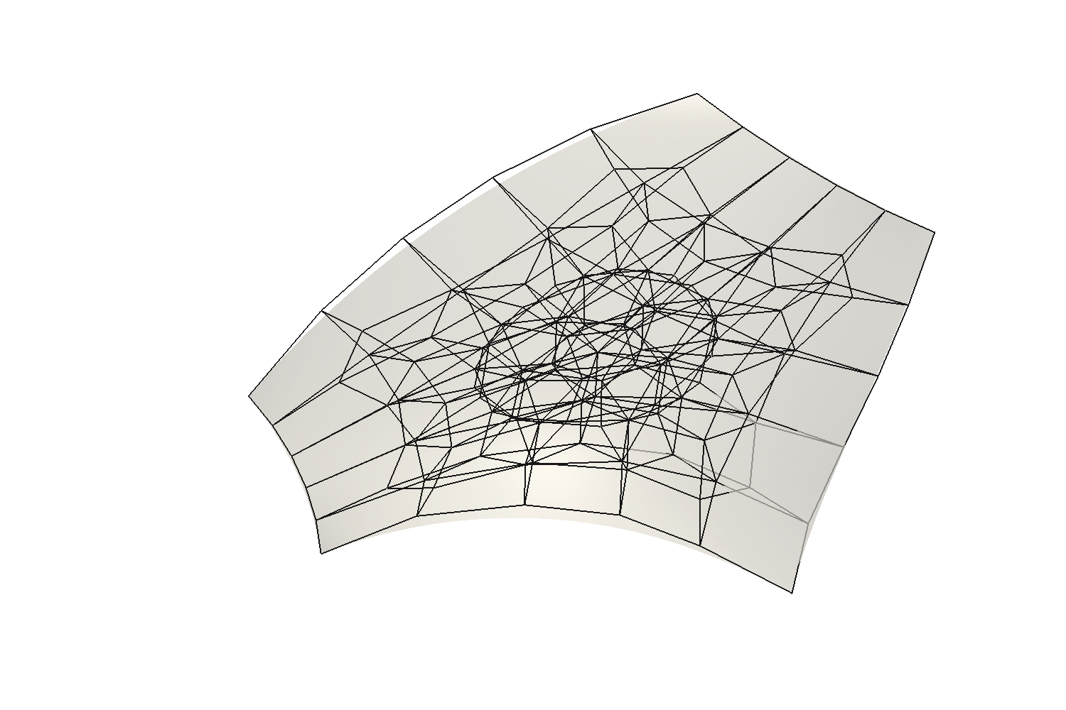
(a) S-patch control network

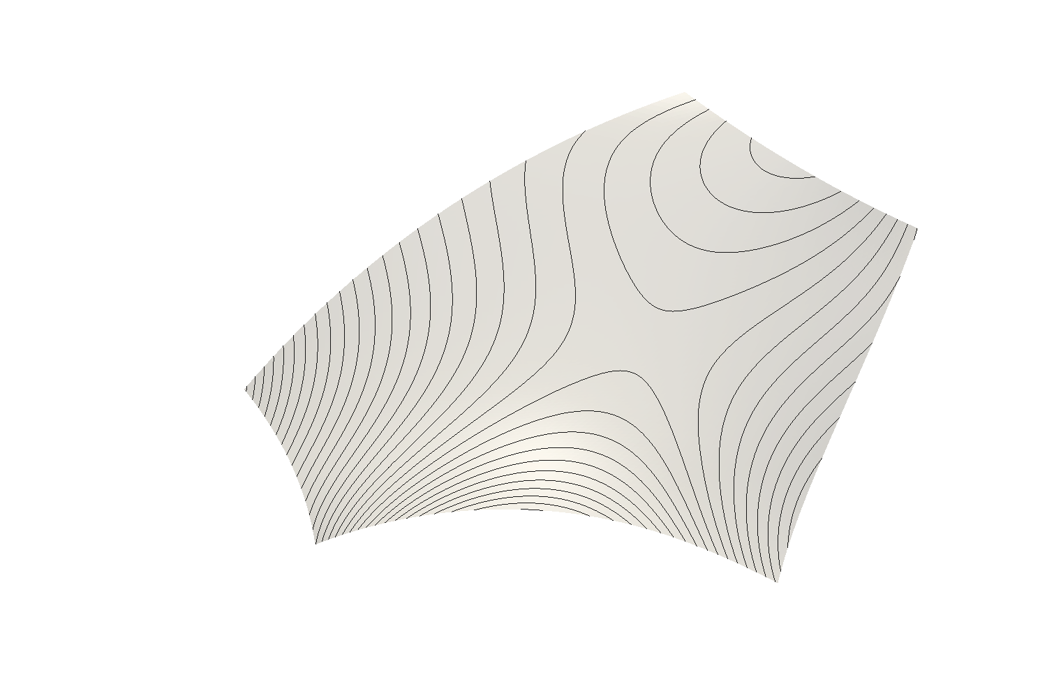
(b) Contouring

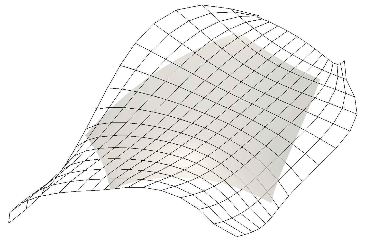
(c) Trimmed patch with control net

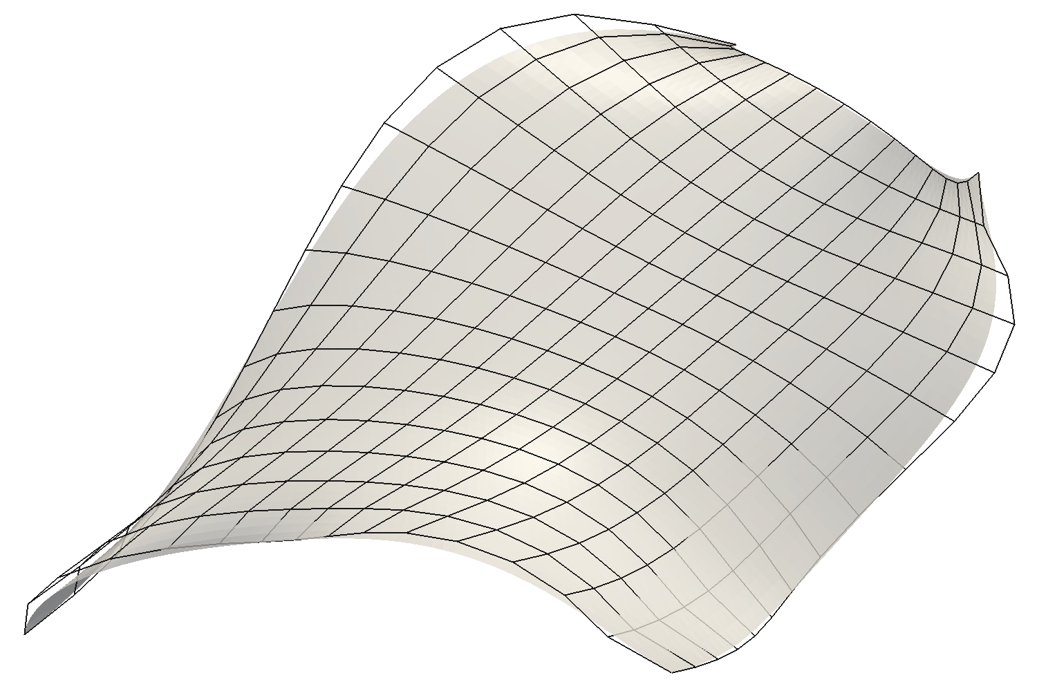
(d) Full tensor product patch

Figure 1: A 5-sided S-patch of depth 5.

6 Discussion

We have seen how S-patches are transformed into trimmed Bézier patches. Let us now look at some practical issues.

6.1 Efficiency

The algorithm in Section 4.1.3 is still computationally demanding. Converting a 5-sided S-patch of depth 8 took more than 5 minutes on a 2.8GHz processor. There is a much faster approach – see the upcoming paper of the author [8].

6.2 Triangles

Three-sided S-patches, i.e., Bézier triangles, are converted into simple polynomial patches, since computing the barycentric coordinates do not involve rational polynomials. Note however, that there are alternative methods for the quadrilateral transformation of a triangular patch, see e.g. Warren’s domain deformation method [10].

6.3 Control net quality

One issue with the conversion is that the quadrilateral control grid may have outlier control points or spikes near the corners. This is because the denominator of Wachspress coordinates vanish on a circle around the domain, and these singularities undermine the stability of these areas.

Conclusion

The S-patch representation of multi-sided surfaces could be an important asset in a modeling toolbox. It can be used to fill holes or create smooth vertex blends, and then it can be exported to CAD/CAM systems as a trimmed Bézier patch, without losing precision, thus making it possible to create perfectly watertight models. In this paper we have reviewed the steps required for the quadrilateral conversion, and discussed some related questions.

References

- [1] Tony D. DeRose. Composing Bézier simplexes. ACM Transactions on Graphics, 7(3):198–221, 1988.
- [2] Tony D. DeRose, Ronald N. Goldman, Hans Hagen, and Stephen Mann. Functional composition algorithms via blossoming. ACM Transactions on Graphics, 12(2):113–135, 1993.
- [3] Kai Hormann and Michael S. Floater. Mean value coordinates for arbitrary planar polygons. Transactions on Graphics, 25(4):1424–1441, 2006.
- [4] Charles T. Loop and Tony D. DeRose. A multisided generalization of Bézier surfaces. ACM Transactions on Graphics, 8(3):204–234, 1989.
- [5] Les A. Piegl and Wayne Tiller. Filling -sided regions with NURBS patches. The Visual Computer, 15(2):77–89, 1999.
- [6] Lyle Ramshaw. Blossoming: A connect-the-dots approach to splines. Digital Equipment Corporation, Palo Alto, 1987.
- [7] Péter Salvi. hole filling with S-patches made easy. In Proceedings of the 12th Conference of the Hungarian Association for Image Processing and Pattern Recognition, 2019.
- [8] Péter Salvi, Tamás Várady, and Alyn Rockwood. Notes on the CAD-compatible conversion of multi-sided surfaces. Computer-Aided Design and Applications (submitted), 2020.
- [9] Márton Vaitkus and Tamás Várady. Parameterizing and extending trimmed regions for tensor-product surface fitting. Computer-Aided Design, 104:125–140, 2018.
- [10] Joe Warren. Creating multisided rational Bézier surfaces using base points. ACM Transactions on Graphics, 11(2):127–139, 1992.