$G^{1}$ hole filling with S-patches made easy

Abstract

S-patches have been around for 30 years, but they are seldom used, and are considered more of a mathematical curiosity than a practical surface representation. In this article a method is presented for automatically creating S-patches of any degree or any number of sides, suitable for inclusion in a curve network with tangential continuity to the adjacent surfaces. The presentation aims at making the implementation straightforward; a few examples conclude the paper.

1 Introduction

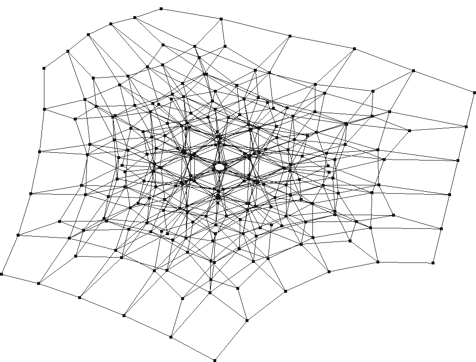
The S-patch [3] is the natural multi-sided generalization of the Bézier triangle. It has various nice mathematical properties, and has been known for a long time, but it has not become a standard surface representation like the tensor product Bézier patch. It is easy to see why: the number of control points grows very fast, and the control network becomes intricate even for surfaces of moderate complexity. For example, a 6-sided quintic patch has 252 control points (see Figure 1), while a tensor product quintic surface has only 36.

Figure 1: The control net of a 6-sided quintic S-patch.

Interactive placement of such a large number of points is hardly possible, but this does not mean that the whole representation should be discarded as impractical. As we will see in the rest of the paper, it is particularly suitable for filling multi-sided holes while ensuring tangential continuity to adjacent surfaces—an important problem in curve network based design.

2 Previous work

A solution for hole filling with S-patches was first presented in [4], where quadratic and cubic surfaces are created based on Sabin nets. Although the equations shown in the paper are also valid for higher degrees, some of the details are left for the reader to figure out. The placement of interior control points, in particular, is not discussed for degrees above cubic.

A recent S-patch-based construction [2] gives a simple mechanism for $G^{1}$-continuous hole filling, even without twist constraints, but only for cubic boundaries. Also, there are no details on the placement of interior control points.

Generalized Bézier (GB) patches [7] present another approach to represent multi-sided Bézier surfaces. Tangential connection to adjacent patches is easily achieved, and its simple control point structure makes it possible to edit the surface interior interactively. On the other hand, some common operations, like analytic derivative computation or exact degree elevation, are difficult or not even possible.

Transfinite surfaces (e.g. [6]) can also be used to fill multi-sided holes when the boundaries are not necessarily Bézier curves; some even have a limited control over the interior.

3 S-patches

An $n$-sided S-patch is defined over an $n$-gon, parameterized by generalized barycentric coordinates $\boldsymbol{\lambda}=(\lambda_{1},\dots,\lambda_{n})$, e.g. Wachspress or mean value coordinates. (In the current paper, we will always use a regular polygon as the domain.) Its control points $\{P_{\mathbf{s}}\}$ are labeled by $n$ non-negative integers whose sum is the degree of the surface ($d$). We will use the notation $L_{n,d}$ for the set of all such labels, and $(s_{1},\dots,s_{n})=\mathbf{s}\in L_{n,d}$ for one particular label. It is easy to see that $|L_{n,d}|=\left(\!\!{n\choose d}\!\!\right)=\binom{n+d-1}{d}$.

The surface point corresponding to a domain point with barycentric coordinates $\boldsymbol{\lambda}$ is defined as

$$S(\boldsymbol{\lambda})=\sum_{\mathbf{s}\in L_{n,d}}P_{\mathbf{s}}\cdot B_{\mathbf{s}}^{d}(\boldsymbol{\lambda})=\sum_{\mathbf{s}\in L_{n,d}}P_{\mathbf{s}}\cdot\frac{d!}{\prod_{i=1}^{n}s_{i}!}\cdot\prod_{i=1}^{n}\lambda_{i}^{s_{i}},$$ (1)

where $B_{\mathbf{s}}^{d}(\boldsymbol{\lambda})$ are Bernstein polynomials with multinomial coefficients.

The labeling system deserves closer inspection. We define the shift operation $\sigma_{j}^{\pm}(\mathbf{s})$ as decrementing $s_{j}$ and incrementing $s_{j\pm 1}$ in label $\mathbf{s}$, e.g. $\sigma_{2}^{+}(1,1,1)=(1,0,2)$ and $\sigma_{1}^{-}(1,0,2)=(0,0,3)$. (Note that label indexing is cyclical.) $P_{\mathbf{s}}$ is said to be adjacent or connected to $P_{\mathbf{\hat{s}}}$, if $\sigma_{j}^{\pm}(\mathbf{s})=\mathbf{\hat{s}}$ for some $j$.

Control points with labels such that $s_{i}+s_{i+1}=d$ are on the $i$-th boundary, e.g. $(0,0,2,3,0,0)\in I_{6,5}$ or $(2,0,0,0,1)\in I_{5,3}$. Specifically, the $j$-th point on the boundary has a label for which $s_{i}=d-j$ and $s_{i+1}=j$, $0\leq j\leq d$ (see Figure 2). We will also refer to these labels by the notation $\mathbf{s}_{i,j}$.

Figure 2: The control net of a 5-sided cubic S-patch with labels. The boundary panels on side 1 are highlighted.

Differentiation of Eq. (1) shows that the first cross derivative at a boundary point is a combination of control points with labels such that $s_{i}+s_{i+1}\geq d-1$ for some $i$. These can be grouped on each side into $d$ boundary panels. The $j$-th panel consists of $n$ points:

$$\mathbf{s}_{i,j},\ \sigma_{j}^{+}(\mathbf{s}_{i,j}),\ \sigma_{j+1}^{+}(\sigma_{j}^{+}(\mathbf{s}_{i,j})),\ \sigma_{j+2}^{+}(\sigma_{j+1}^{+}(\sigma_{j}^{+}(\mathbf{s}_{i,j}))),\ \dots,$$

until we get back to $\mathbf{s}_{i,j}$. The $k$-th point of this panel is also denoted by $P_{j,k}^{i}$, so $P_{j,2}^{i}=P_{j+1,1}^{i}$. For example, in the five-sided cubic patch in Figure 2, $\{P_{2,k}^{3}\}$ contains control points with labels $(0,0,1,2,0)$, $(0,0,0,3,0)$, $(0,0,0,2,1)$, $(1,0,0,2,0)$, and $(0,1,0,2,0)$.

(a) Boundary constraints

(b) $G^{1}$ boundary panels

(c) Interior control points

Figure 3: Stages of filling a five-sided hole with quintic boundary constraints.

4 Hole filling

Now that S-patches are defined, we can turn our attention to the $n$-sided hole filling problem. Let the boundary curves be given in Bézier form, with a common degree $d$. Cross-derivative constraints are represented by a second row of control points on all sides; the two control rows together are called a Bézier ribbon [7]. We need to construct a surface that matches, for each side, the derivatives of a $d\times d$-degree tensor product Bézier patch with the same two control rows, see Figure 3a.

Let $C_{j,k}^{i}$ denote the $j$-th control point in the $k$-th row on the $i$-th side ($1\leq i\leq n$, $0\leq j\leq d$, $0\leq k\leq 1$). We assume that the constraints are twist-compatible, i.e., $C_{1,1}^{i}=C_{d-1,1}^{i-1}$, $C_{1,0}^{i}=C_{d,1}^{i-1}$ and $C_{0,1}^{i}=C_{d-1,0}^{i-1}$ for each $i$ (using cyclic indexing). This form of the boundary constraints is called a Sabin net in [4].

The rest of this section will describe how to compute the correct boundary panels for $G^{1}$ interpolation of the cross-derivatives (Figure 3b), and how to set the position of the remaining control points automatically (Figure 3c).

4.1 $G^{1}$ boundaries

This section is based on [4], where the derivation of these equations can be found. In the paper explicit formulas are only given for the special cases of $d=2$ and $3$; here we will look at the general degree case for the convenience of the reader.

Before diving into the intricacies of tangential continuity, it is important to note that the boundaries of an S-patch are Bézier curves with $P_{j,1}^{i}$ ($0\leq j\leq d$) as the control polygons, so if positional ($C^{0}$) interpolation is enough, it can be done by setting $P_{j,1}^{i}=C_{j,0}^{i}$ for every $i$ and $j$.

The conditions of tangential continuity with a Bézier triangle (or another S-patch) of the same degree are simple: (i) each boundary panel should be the affine image of the domain polygon, and (ii) opposite boundary panels along the common boundary should be in the same plane.

From (i) it follows that it suffices to set 3 points of each panel, 2 of which are on the boundary, so only one extra point is needed, e.g. $P_{j,n}^{i}$. The $n$-sided setting introduces additional constraints, which can be satisfied only with an S-patch of degree $d+3$. Eventually we arrive at the equation

$$P_{j,n}^{i} =P_{j,1}^{i}+\frac{d}{(d+3)}\left[\delta_{1}^{d}(j)\left(C_{j,0}^{i}-C_{j-1,0}^{i}\right)\cdot 2c\binom{d-1}{j-1}+\right.$$

$$\qquad\qquad\qquad\qquad\delta_{2}^{d+1}(j)\left(C_{j-1,0}^{i}-C_{j-2,0}^{i}\right)\cdot 4c\binom{d-1}{j-2}+$$

$$\qquad\qquad\qquad\qquad\delta_{3}^{d+2}(j)\left(C_{j-2,0}^{i}-C_{j-3,0}^{i}\right)\cdot 2c\binom{d-1}{j-3}+$$

$$\qquad\qquad\qquad\qquad\delta_{0}^{d}(j)\left(C_{j,1}^{i}-C_{j,0}^{i}\right)\cdot\binom{d}{j}+$$

$$\qquad\qquad\qquad\qquad\delta_{1}^{d+1}(j)\left(C_{j-1,1}^{i}-C_{j-1,0}^{i}\right)\cdot(2+2c)\binom{d}{j-1}+$$

$$\left.\qquad\qquad\qquad\qquad\delta_{2}^{d+2}(j)\left(C_{j-2,1}^{i}-C_{j-2,0}^{i}\right)\cdot\binom{d}{j-2}\right]/\binom{d+2}{j},$$ (2)

where $c=-\cos(2\pi/n)$ and

$$\delta_{l}^{h}(j)=\begin{cases}1&l\leq j\leq h\\ 0&\text{otherwise}\end{cases}$$ (3)

(The boundary control points $P_{j,1}^{i}$ can be computed as in the $C^{0}$ case, after degree elevating the Bézier ribbon 3 times.)

The remaining control points in a panel are computed by the affine transformation. After solving

$$\left[\begin{array}[]{ccc}1&0&1\\ \cos(2\pi/n)&\sin(2\pi/n)&1\\ \cos(4\pi/n)&\sin(4\pi/n)&1\end{array}\right]\cdot M^{T}=\left[\begin{array}[]{c}(P_{j,n}^{i})^{T}\\ (P_{j,1}^{i})^{T}\\ (P_{j,2}^{i})^{T}\end{array}\right]$$ (4)

for $M^{T}$, we get

$$P_{j,k}^{i}=M\cdot\left[\begin{array}[]{ccc}\cos(2k\pi/n)&\sin(2k\pi/n)&1\end{array}\right]^{T}.$$ (5)

4.2 Interior control points

There are various heuristics for the placement of interior control points, mainly for lower-degree patches. The procedure presented here works for any S-patch, independently of the number of sides, the degree, or the type of continuity. It is based on the work of Farin et al. [1], which shows that applying discrete masks on the control network of a tensor product Bézier surface can result, depending on the masks used, in a Coons patch or a quasi-minimal surface. Monterde et al. [5] investigated harmonic and biharmonic masks, and these are easily applicable to S-patches, as well.

Table 1a shows the harmonic mask. For a tensor product Bézier patch with control points $Q_{i,j}$, this represents the equation system

$$Q_{i+1,j}+Q_{i-1,j}+Q_{i,j+1}+Q_{i,j-1}-4Q_{i,j}=0,$$ (6)

i.e., each control point should be the average of its neighbors. If we fix the outermost control rows, the system can be solved, resulting in a smooth distribution of points. This can be directly applied to S-patches, using the adjacency relation defined in Section 3. Note, however, that there can be different masks even within one patch, as the valency of control points may vary.

	0	1	0
	1	-4	1
	0	1	0

(a) Harmonic mask

0	0	1	0	0
0	2	-8	2	0
1	-8	20	-8	1
0	2	-8	2	0
0	0	1	0	0

(b) Biharmonic mask

Table 1: Masks used on tensor product Bézier control networks. The number in bold is the coefficient of the control point the mask is applied to.

When the cross-derivatives are fixed at the boundary, it is natural to use a biharmonic mask (see Table 1b). This is computed by applying the harmonic mask on itself, which translates to S-patches in a straightforward way, see Algorithm 1. All examples in this paper were computed by this method.

harmonicMask(i):

xxneighbors = indices adjacent to i

xxfor j in neighbors:

xxxxmask[j] = 1

xxmask[i] = -length(neighbors)

xxreturn mask

biharmonicMask(i):

xxmask = 0 for all indices

xxfor (j,wj) in harmonicMask(i):

xxxxfor (k,wk) in harmonicMask(j):

xxxxxxmask[k] += wj * wk

xxreturn mask

Algorithm 1 Computing harmonic and biharmonic masks.

5 Examples

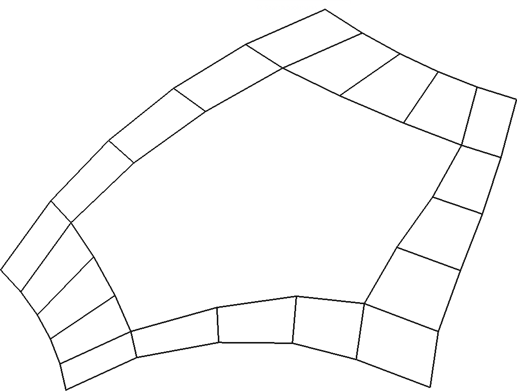
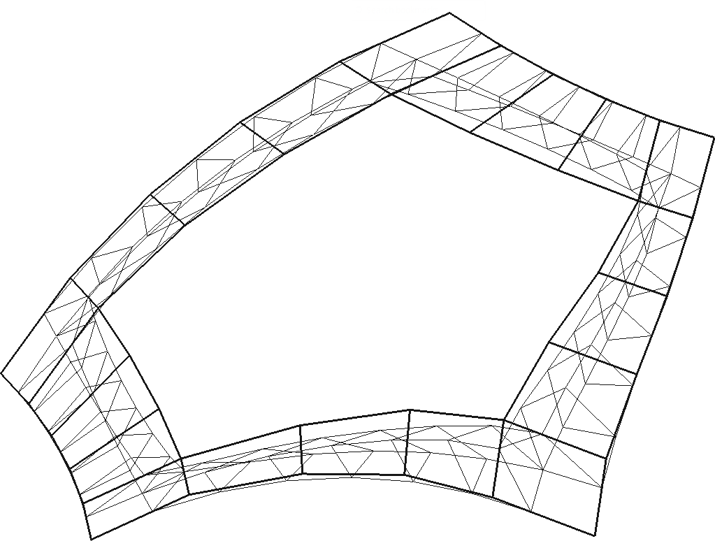
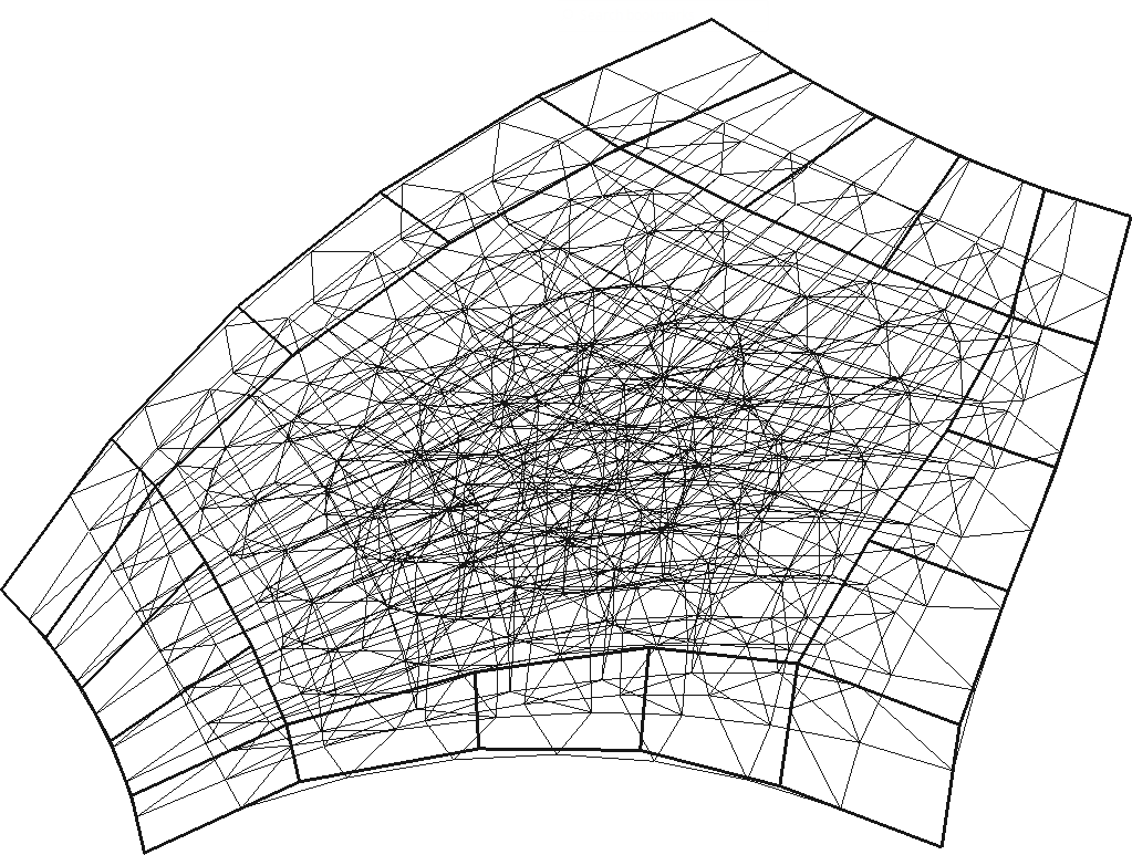
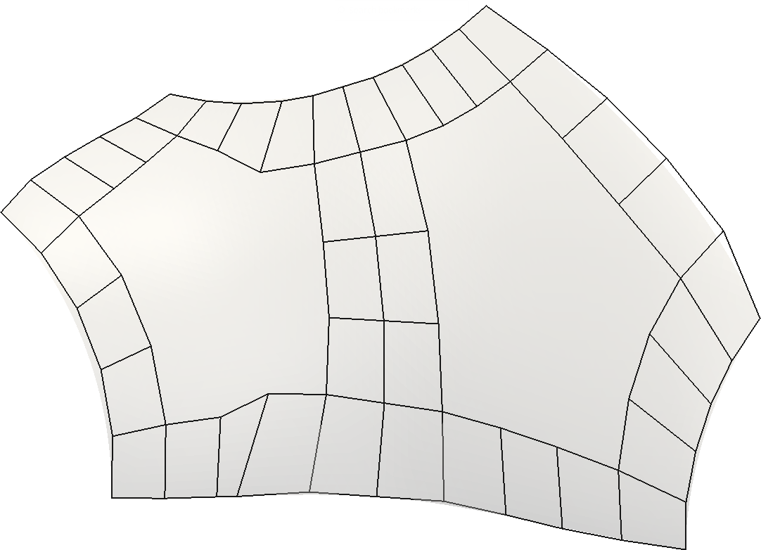
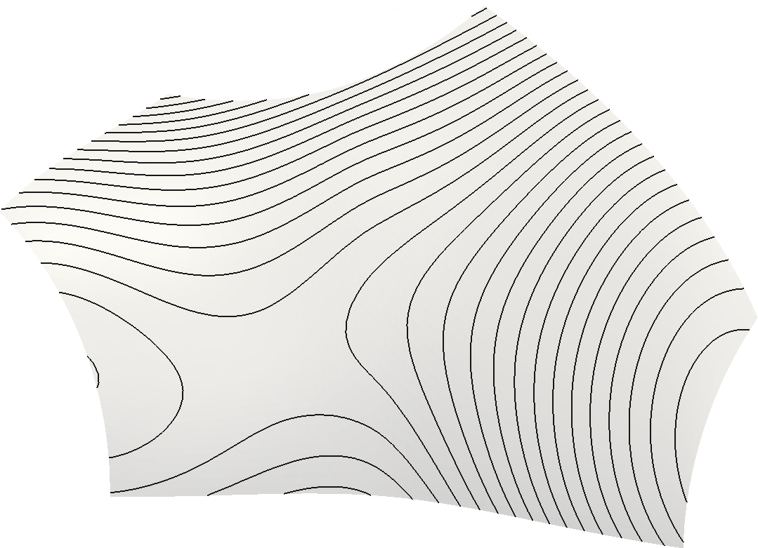
Surface quality of S-patches generated by the above procedure are generally very good, an example is shown in Figure 4. The 5-sided quintic Bézier ribbon comprises 40 control points, while the degree-elevated S-patch has 495 points (135 in boundary panels, 360 in the interior).

$G^{1}$ connection between adjacent surfaces is illustrated in Figure 5.

Figure 4: Isophotes of the surface shown in Figure 3c.

Figure 5: S-patches connected with $G^{1}$ continuity (left: ribbons, right: contours).

Conclusion and future work

We have seen that S-patches can be useful as surfaces filling boundary loops in curve networks. An explicit construction was shown that achieves tangential continuity with adjacent surfaces by fixing the boundary panels of the patch. For the placement of the unconstrained control points, a new algorithm was presented that can be used with surfaces of any degree.

There are several interesting questions remaining, such as the effect of the masks on the surface (does it minimize some functional?), or a generalization to curvature continuous connections.

References

- [1] Gerald Farin and Dianne Hansford. Discrete Coons patches. Computer Aided Geometric Design, 16(7):691–700, 1999.
- [2] Gerben J. Hettinga and Jiří Kosinka. Multisided generalisations of Gregory patches. Computer Aided Geometric Design, 62:166–180, 2018.
- [3] Charles T. Loop and Tony D. DeRose. A multisided generalization of Bézier surfaces. ACM Transactions on Graphics, 8(3):204–234, 1989.
- [4] Charles T. Loop and Tony D. DeRose. Generalized B-spline surfaces of arbitrary topology. In 17th Conference on Computer Graphics and Interactive Techniques, SIGGRAPH, pages 347–356. ACM, 1990.
- [5] Juan Monterde and Hassan Ugail. On harmonic and biharmonic Bézier surfaces. Computer Aided Geometric Design, 21(7):697–715, 2004.
- [6] Péter Salvi, István Kovács, and Tamás Várady. Computationally efficient transfinite patches with fullness control. In Proceedings of the Workshop on the Advances of Information Technology, pages 96–100, 2017.
- [7] Tamás Várady, Péter Salvi, and György Karikó. A multi-sided Bézier patch with a simple control structure. Computer Graphics Forum, 35(2):307–317, 2016.