Stellar mass measurements in Abell 133 with Magellan / IMACS

Abstract

We present the analysis of deep optical imaging of the galaxy cluster Abell 133 with the IMACS instrument on Magellan. Our multi-band photometry enables stellar mass measurements in the cluster member galaxies down to a mass limit of $M_{\star}=3\times 10^{8}\,M_{\odot}$ ($\approx 0.1$ of the Large Magellanic Cloud stellar mass). We observe a clear difference in the spatial distribution of large and dwarf galaxies within the cluster. Modeling these galaxies populations separately, we can confidently track the distribution of stellar mass locked in the galaxies to the cluster’s virial radius. The extended envelope of the cluster’s brightest galaxy can be tracked to $\sim 200$ kpc. The central galaxy contributes $\sim 1/3$ of the the total cluster stellar mass within the radius $r_{500c}$.

Draft version

1 Introduction

Clusters of galaxies have total gravitating masses of $\sim 10^{14}-10^{15}\ M_{\odot}$ and are the most massive systems that have had time to collapse in the standard $\Lambda$CDM cosmology (see Kravtsov & Borgani, 2012, for a review). Given a mean comoving density of matter in the universe of $\approx 4\times 10^{10}\,M_{\odot}\,\rm Mpc^{-3}$, the large cluster masses imply that their matter was assembled from regions of $\sim 15-50\,\rm Mpc$ in size. Although clusters tend to form in high-density regions (Kaiser, 1984), the vast scales involved in their formation means that, at least within roughly the virial radius, the enclosed matter should have a mix of baryons and dark matter close to the universal value (e.g., White et al., 1993; Frenk et al., 1999; Valdarnini, 2003; Kay et al., 2004; Kravtsov et al., 2005). Furthermore, the sizes of their virialized regions after collapse are $R\sim 1-5$ Mpc and their binding energies, $GM^{2}/R$, are thus $\sim 10^{63}-10^{64}$ ergs. Therefore, even the most energetic Active Galactic Nuclei (AGN) feedback cannot eject baryons from deep potential wells of clusters and significantly lower their baryon mass fraction (e.g., Planelles et al., 2013; Battaglia et al., 2013; Henden et al., 2018). This means that clusters should be approximately closed systems.

Studies of the total baryon fractions in clusters can thus be used as a valuable test of the overall structure formation paradigm (see, e.g., Allen et al., 2011, for a review). At the same time, baryon mass fractions within the radii readily accessible by current X-ray observations, $\sim 0.5$ of the virial radius, are well below the values of the universal baryon fraction derived from Cosmic Microwave Background fluctuations (Vikhlinin et al., 2006; Lin et al., 2012; Eckert et al., 2016), and this is yet to be fully explained by cosmological cluster simulations (e.g., Barnes et al., 2017). Furthermore, the distribution of stellar material and hot gas within clusters should bear the imprint of key processes shaping galaxy formation. Indeed, observed stellar mass fractions and stellar mass function of cluster galaxies have become valuable benchmarks for testing models of feedback in cosmological simulations of cluster formation (e.g., Martizzi et al., 2014, 2016; Bahé et al., 2017; McCarthy et al., 2017; Cui et al., 2018; Pillepich et al., 2018; Henden et al., 2018). The radial profile of stellar density of the Brightest Cluster Galaxy (BCG), as well as the radial distribution of stellar mass in galaxies are potentially equally powerful constraints on the models (e.g., Martizzi et al., 2014; Bellstedt et al., 2018).

Despite recent progress (Gonzalez et al., 2013; Budzynski et al., 2012, 2014; Kravtsov et al., 2018; Huang et al., 2018), the number of clusters with available accurate measurements of the gas mass, stellar mass in galaxies down to dwarf scales, and stellar material in the outer envelope of the central galaxy remains small. The main goal of this study is to accurately measure the contribution of the stellar populations (individual galaxies and intra-cluster light) to the total baryon budget in the cluster Abell 133.

Abell 133 is a massive nearby ($z=0.05695$) galaxy cluster with extensive mapping of surrounding distribution of galaxies and filamentary cosmic web structure (Connor et al., 2018, 2019b), as well as deep X-ray observations by the Chandra X-ray Observatory (Vikhlinin et al., 2006; Vikhlinin, 2013; Morandi & Cui, 2014, Vikhlinin et al., in preparation). The cluster has a cool core and prominent radio relics indicative of the ongoing merger activity (Randall et al., 2010), although distribution of galaxies does not reveal clear signs of dynamical disturbance (Connor et al., 2018). Hydrostatic equilibrium analysis using X-ray Chandra observations give total mass within the radius enclosing density contrast equal to the 500 times the critical density at the redshift of the cluster of $M_{500c}\approx 3.42\times 10^{14}\,M_{\odot}$ and corresponding radius $r_{500c}=1.048\,\rm Mpc$.

The paper is organized as follows. In Section 2 we explain the choice of fields within A133 and neighboring fields used to estimate background galaxy density, describe observations of these fields using the IMACS camera on the 6.5m Magellan Baade telescope and present their images and general discussion of the features they reveal.

In Section 3 we describe data reduction procedures, assumptions, and methods we use to carry out source detection, classification, galaxy photometry, and sample completeness. In Section 4 we describe the method we use to estimate stellar masses from galaxy luminosities and colors (§4.1) and results pertaining to the stellar mass function (§4.2). In Section 5 we present the radial distribution of galaxies of different stellar mass (§5.1), the radial stellar mass distribution of the BCG (§5.2) and the total mass profile of all stars in the cluster (§5.3). We discuss our findings and their interpretation in Section 6 and summarize our main results and conclusions in Section 7.

All distant-dependent quantities throughout this paper are computed assuming the nominal best-fit cosmological parameters from Bennett et al. (2014): $h=0.696$, $\Omega_{\rm M}=0.286$, and $\Omega_{\rm\Lambda}=0.714$. Galaxy luminosities are computed in the rest-frame using the Vega magnitude system.

2 Observations

The galaxy cluster A133 was observed on the 6.5m Magellan Baade Telescope over three nights in 2005. The observations were performed with the IMACS (Inamori-Magellan Areal Camera and Spectrograph, Dressler et al., 2011) instrument in its f/2 focus configuration with the 8192$\times$8192 pixel Mosaic1 detector. The central cluster region and South-East extension were covered with a six-location grid (Figure 1). The coverage reaches outside the $r_{200c}$ radius in the West, South, and South-West directions from the cluster center. Unfortunately, the North-East corner of the cluster remained unobserved. In analyzing the galaxy distributions below, we make an assumption of azimuthal symmetry.

Since the fore- and background galaxy populations have to be subtracted statistically in the cluster pointings, we obtained data for their careful calibration. Specifically, we observed 8 background fields at $\sim 1.5^{\circ}$ ($\approx 6\,$Mpc) distances from the cluster center. Approximately half of all available exposure time was spent in these background fields, so the background images reach the same depth as the A133 pointings. Also, we constantly alternated between the cluster and background fields during the night, so the background pointings can be used for a measurement of the diffuse sky background. This turned out to be crucial for analyzing the extended diffuse light halo of the cluster central galaxy (see § 5.2 for details). We chose to observe the fields for background estimation at $6\,\mathrm{Mpc}\approx 3.5r_{200c}$, as opposed to using random pointings far away from the cluster, because most of the volume at $z\sim 0$ is in low-density regions. At the same time, galaxies and mass are strongly correlated with clusters and the average profile of mass around clusters is expected to reach mean density only at $\gtrsim 10R_{\rm vir}$ (e.g., Diemer & Kravtsov, 2014). Significant contribution to the relevant projected background is thus expected to be due to such correlated structures relatively close to the cluster, while commonly used estimates of the background using random fields will underestimate the background (see, e.g., discussion in §2.2.3 of Busch & White, 2017). Therefore, we chose to estimate background at the radii well outside the virial radius, but still sufficiently close to the cluster to give us a realistic estimate of the background population.

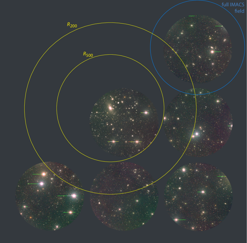
Figure 1: Mosaic of IMACS observations of A133, blending the images in the $R$, $V$, and $I$ filters. Only the inner 20 arcmin diameter regions of each field were used in the analysis (§ 3.2) and are shown here. The full IMACS field of view (27.4 arcmin diameter) is shown by the blue circle for guidance. Yellow circles mark $r_{500c}$ and $r_{200c}$ radii of the cluster. Note that all data shown in this image are the “cluster” fields. We have obtained an additional set of 8 background fields (not shown here) at $\sim 1.5^{\circ}$ off-cluster distances.

All fields were observed in the Bessel $V$, Bessel $R$, and CTIO $I$ filters. In each filter, several exposures were taken with $\sim 15^{\prime\prime}$ dither to facilitate removal of cosmic rays and cosmetic defects of the CCDs. The total exposure per location per filter was in the range from 300 to 1800 sec. The deepest images were taken in the $R$-band (typical exposures $\sim 900$ sec), while $V$- and $I$-band images are shallower (typically, 300 sec). The deepest exposures were taken for the central cluster field and one of the background fields — 1800, 1500 and 900 sec in $R$, $V$, and $I$ filters, respectively. Seeing varied during the observing run in the range $0.6^{\prime\prime}-1.2^{\prime\prime}$, but stayed sub-arcsec for a large fraction of the $R$-band observations. For accurate photometric calibration, we observed the standard star field SA 98 Landolt (1992) in $R$, $V$, and $I$ filters in the pre-dawn hours of each night.

When this paper was in preparation, the first release of the DES (Dark Energy Survey DES Collaboration, 2018) data near the A133 location became available. The DES data cover a larger area around the cluster and provide accurate photometry in the SDSS filters. However, we find that the DES images are shallower than our Magellan data (see Figure 3 below). We, therefore, used the DES catalogs to verify the accuracy of photometric measurements and stellar mass determinations from Magellan data for commonly detected galaxies (see § B).

2.1 General discussion of Magellan images

The composite Magellan image (Figure 1) clearly shows a large number of A133 member galaxies. The cluster is dominated by the brightest central galaxy. We show below that the BCG, including its extended envelope, contributes over 30% of the total stellar mass in the cluster within $r_{500c}$ and $\sim 50\%$ within $0.5\,r_{500c}$ (§ 5.3). There are a few other structures worthy of a brief discussion.

In Figure 2, we show a zoom-in on the cluster central region. The colors represent the relative flux in the $V$, $R$, and $I$ bands, and are chosen such the color of galaxies on the A133’s red sequence is white. In addition to a large number of A133 members, the image clearly shows a concentration of fainter, red galaxies $\sim 150$ kpc to the South-East of the BCG. This group of galaxies forms a separate red sequence and corresponds to a background galaxy cluster at $z\approx 0.29$ (see § 3.4 below).

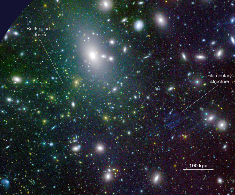
Figure 2: Zoom-in on the central region of A133. North is up, East is to the left, and the colors in the $V$, $R$, and $I$ blend are chosen so that the A133 red sequence corresponds to white. Approximately $\sim 300$ kpc South-West of the BCG there is a filamentary structure with bluer colors than the population of A133 ellipticals. Approximately 150 kpc to the South-East of the A133 BCG there lies a projected background cluster ($z=0.29$), apparent as a group of redder galaxies (§ 3.4).

At a distance of $\sim 300$ kpc to the South-West of the BCG, there is a filamentary structure with bluer colors than the A133 elliptical galaxies. This structure possibly corresponds to a tidally disrupted cluster member. It has a size of $~{}100$ kpc, apparent magnitude $R=19.8$ mag, and color $V-R=0.19$ mag, $\approx 0.3$ mag bluer than the A133 red sequence (c.f. Figure 9 below). Other examples of tidally disrupted galaxies in nearby clusters have been reported, such as UGC 6697 in A1367 (Sun & Vikhlinin, 2005) and ESO 137-001 in A3627 (Sun et al., 2007). These objects show $\sim 50$ kpc tails of H$\alpha$ and X-ray emission. The filamentary structure in A133 is larger in size, and does not show any X-ray tails in the sensitive Chandra data (no narrow-band H$\alpha$ imaging is available at the time of this writing). Further analysis of these structures will require additional data.

3 Data Analysis

3.1 Basic Image Reduction

Basic data reduction steps including bias removal, dark current correction, and flat fielding using twilight flats were performed with IRAF’s CCDPROC package. Individual images in each dither pattern were merged using a combination of mean and median averaging with sigma-clipping. This procedure automatically removes the cosmic rays and cosmetic CCD defects.

The astrometric solutions were obtained using the Astrometry.net package (Lang et al., 2010). All images were then resampled to a common tangential projections. This step was necessary for accurate matching of the images obtained in individual filters and for creating large-scale mosaics such as those shown in Figure 1. Because the IMACS f/2 camera was slightly misaligned prior to adjustments made in 2006 and 2008, resampling to a global tangential projection resulted in small aliasing effects. Those effects have not seriously affected the image quality because the image pixel size, $0.2^{\prime\prime}$, is substantially smaller than the seeing during the A133 observing run. However, aliasing modifies the pixel-to-pixel noise in the final images, and has to be taken into account during object detection (see § 3.3.1 and Appendix A below).

3.2 Background Subtraction

To accurately calculate fluxes of bright and faint sources, we use global and local background subtraction methods. Sky brightness and noise levels heavily varied among images of the same exposure in a given field. However, we noticed that for every image, there was a linear dependence between sky brightnesses in the center and the center-to-edge difference. This dependence was exploited to remove the time variations of the background. Therefore, we could build a combined background image from all observed background fields taking into account individual levels of noise and sky, and excluding point sources. This image, the global background pattern, was subtracted from all observations. Unfortunately, using this method we could not model random spatial variations of the background which appear in some fields. We applied local background subtraction method to produce images which we used for detection and flux measurements for majority of sources (see Appendix A for a description of this procedure).

Individually processed images were combined into the final master images for every cluster and background field. The IMACS CCD camera ideally delivers an 27.4 arcmin diameter field. However, there was substantial loss of image quality (coma and astigmatism) near the edge of the field of view prior to 2008, in addition to substantial vignetting. We also found that the background pattern near the field edge was unrepeatable, which was problematic for global background subtraction. Therefore, we reduced the diameters of our fields to 20 arcmin.

The bright, saturated stars render a portion of the cluster field unusable for detection of faint sources and accurate galaxy photometry. We masked out such regions ($\sim 40^{\prime\prime}$ radius) and excluded them from all further analysis. This excludes $\sim 3\%$ of the overall image area. More extended wings around bright stars are properly subtracted by our local background subtraction procedure.

3.3 Source Detection & Photometry

Our general strategy was to detect sources and measure galaxy fluxes in the $R$ band, and then measure fluxes at the same locations and within the same apertures in the $V$ and $I$ bands. Our procedure, detailed below, was designed to compensate for the difference in sensitivity and seeing in different filters and cluster locations, and to ensure accurate photometry even for very faint galaxies.

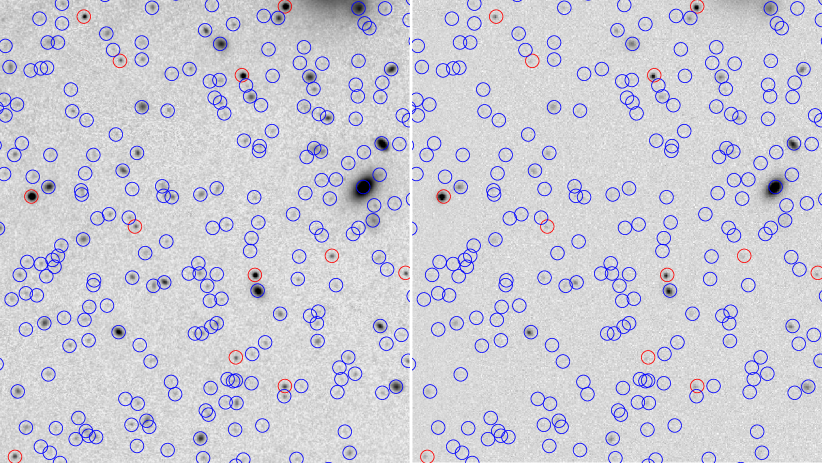
Figure 3: Illustration of the wvdecomp-based detection in one of the cluster fields (circles). Blue circles are galaxies; red circles are stars identified by SExtractor. The left panel shows our $R$-band Magellan image. The right panel shows the $r$-band DES image of the same region, with Magellan detections superimposed.

3.3.1 Source Detection

We start with running a source detection algorithm on the combined $R$-band images. We used the wavelet decomposition algorithm, wvdecomp, which is proven to be very efficient for detection of faint extended sources in X-ray images (Vikhlinin et al., 1998). We computed the noise map to properly set detection thresholds at each location. This is crucial for analyzing the faint galaxies in our Magellan images because pixel-to-pixel noise varies strongly within the field due to aliasing (see above) and non-uniform exposure coverage. The noise maps were empirically created from the data by convolving images cleaned from sources with the wvdecomp’s wavelet kernel and averaging the resulting rms deviations on $6^{\prime\prime}$ spatial scales (see Appendix A for details). wvdecomp uses this map for detection on the smallest scales; when proceeding to the largest scales, the noise map is appropriately smoothed further by the software (see Vikhlinin et al., 1998, for details).

The output from wvdecomp is locations of statistically significant sources (Figure 3). We need a separate software package to apply additional selection criteria and measure galaxy fluxes. The first step is to identify and remove the likely stellar sources. To this end, we have run the SExtractor (Bertin & Arnouts, 1996) detection on our $R$-band images, cross-matched the SExtractor and wvdecomp source lists, and removed sources for which SExtractor measured stellarity indices $>0.9$. On average $\approx 4\%$ of sources detected by wvdecomp were removed by this procedure.

3.3.2 Fluxes and colors

Our main goal with the galaxy photometry is to reliably determine total luminosities for galaxies of different types and down to low fluxes. We also need to ensure that the flux measurements are consistent between exposures obtained in different filters and under different seeing conditions. Our approach is as follows. We assume that there are no color gradients within individual galaxies, as seems to be the case for outer regions of massive spheroidal galaxies (see, e.g., La Barbera et al., 2010; D’Souza et al., 2014). We fit the observed $R$-band (best-exposed filter) surface brightness profiles of each galaxy with an analytic model that includes the PSF effects. This analytic fit is used to define the circular aperture size for subsequent flux measurement and determine the aperture correction. The apertures are chosen such that they are reasonably small to ensure good signal-to-noise in the flux measurements. At the same time, they are sufficiently large such that the differences in seeing between different nights and filters lead to negligible changes in the aperture correction factors.

The galaxy profiles were extracted in circular annuli, centered on the surface brightness peak determined by wvdecomp. The annuli were of a constant log-width ($\lg(r_{\mathrm{max}}/r_{\mathrm{min}})=0.15$), with a maximim radius equal to 1.5 times the maximum distance from the source within this source’s “island” (see Appendix A). The profiles exclude other sources detected in the vicinity by masking out the image pixels falling within these other sources’ islands and scaling the measured flux in the partially-masked annulus appropriately.

Our analytic model is motivated by the results of Kravtsov (2013), who showed that the stellar surface density profiles of galaxies of different morphological types have approximately similar shape at radii $r\gtrsim r_{n}$ and largely differ at $r\lesssim r_{n}$, where $r_{n}$ is approximately a half mass radius of stellar distribution. Within that radius, the profile of early-type galaxies is approximately described by the de Vaucouleurs model, while the late-type galaxies follow the exponential profile. We further note that Sersic-type function, $I(r)\propto\exp(-7.669\,(r/r_{0})^{\gamma})$, can describe both the de Vacouleurs model and the exponential model, depending on the values of $r_{0}$ and $\gamma$. The Kravtsov (2013) results indicate that the Sersic index, $\gamma$, is not constant with radius, but is changing near the radius $r_{n}$. We can approximate this by replacing $r/r_{0}$ with a function $z=y^{\alpha}(1+y^{2})^{1-{\alpha}/2}$, where $y=r/r_{0}$. In this case, the effective Sersic is $\gamma$ for $r\gg r_{0}$, and $\gamma\,\alpha$ for $r\ll r_{0}$.

To account for the PSF effects, one ideally needs to convolve a 2D light distribution with a Gaussian, and then convert the result back to the 1D radial profile. This approach is very computationally-intensive. We found that instead of the 2D convolution, the PSF effects can be sufficiently accurately approximated by multiplying the profile by $\mathrm{erf}(r/p)$ where $p$ is a free parameter fit individually for each galaxy. At $r\gg p$, this does not modify the profile, while at $r\ll p$, it introduces a flattening. Qualitatively, these are precisely the modifications expected from finite seeing.

To summarize, our analytic model is

$$I(r)=I_{0}\exp(-7.669\,z^{\gamma})\,\times\,\mathrm{erf}(r/p),$$ (1)

where $z=y^{\alpha}(1+y^{2})^{1-{\alpha}/2}$, $y=r/{r_{0}}$, and $I_{0},r_{0},\alpha,\gamma,p$ are model parameters. We found that this model provides an accurate approximation to the data. The structural parameters ($r_{0}$, etc.) can not be used literally because we treat the PSF effects approximately. However, the total galaxy luminosities can be obtained accurately, which is our goal. Examples of how this model fits the profiles of typical spiral and elliptical galaxies in our observations are shown in Figure 4–5.

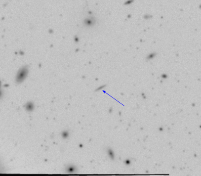
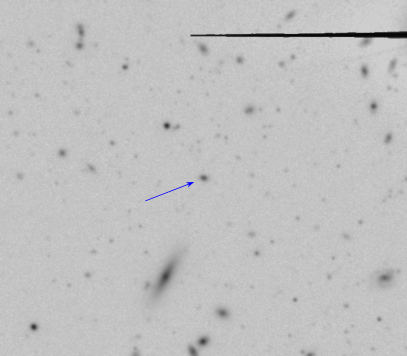
(a)                                                        (b)

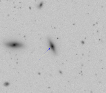
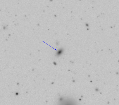
(c)                                                        (d)

Figure 4: Examples of galaxies whose profiles and best-fit models are shown in Figure 5. Examples include bright and faint spirals and ellipticals.

(a)                                                        (b)

(c)                                                        (d)

Figure 5: Surface brightness profiles and best fit models (Eq. 1) for the galaxies shown in Figure 4. These examples include both spirals (a and c) and ellipticals (b and d).

To check that the method for flux measurement is accurate and stable, we performed the following test. The profile of Eq. 1 with parameters fit to the $R$-band images for each galaxy was used to compute radii enclosing 50%, 70%, etc. of the total light. We then measured the actual flux within these radii and estimated total flux, as, e.g., $f_{\mathrm{tot}}=f_{50}/0.5$ and compared such estimate with the $f_{\mathrm{tot}}$ computed using the analytic profile. If our model provides an accurate description of the observed profiles, and the PSF effects are treated sufficiently accurately, the two estimates of $f_{\mathrm{tot}}$ should agree and such comparison thus represents a test of the accuracy of the model of eq 1. In Figure 6 we show an excellent agreement of $f_{\mathrm{tot}}$ fluxes based on measurements in the $r_{50}$ and $r_{70}$ radii. Since all aperture definitions work equally well, we use the $r_{50}$-based fluxes in the further analysis, to maximize signal-to-noise.

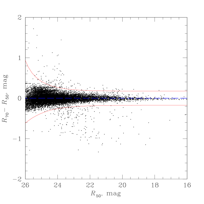
Figure 6: Comparison of the apparent $R$-band magnitudes of galaxies in the central cluster field, based on the aperture fluxes and correction factors for $r_{50}$ and $r_{70}$ radii (see text). For the majority of objects, there is an excellent agreement of the two measurements, with a small scatter shown by the solid red lines. There is a small percentage of outliers outside of the main relations indicated by red lines to guide the eye. We have hand-checked a large number of those. The outliers with the positive deviations of the $r_{70}$-based magnitudes were all found to be spurious detections in the wings of bright stars and galaxies. They were eliminated from further analysis. The systematic offset between the two fluxes is only $0.03$ mag.

To compute colors for each galaxy, we calculate the fluxes in the other filters using the apertures from the R-band, our deepest images. The same aperture corrections are applied to all filters. This is equivalent to an assumptions of no color gradients within individual galaxies; the central cluster galaxy is the only object where we accounted for the color gradients explicitly (see § 5.2 below). However, we need to apply an extra care in selecting the aperture size, because the seeing for data obtained in different filters can vary. We assume the PSF-related effects on the galaxy brightness profiles are small outside the radius equal to the FWHM of the PSF in that observation. Therefore, the galaxy aperture was selected as the maximum of $r_{50}$ and the PSF FWHM’s for observations of the given field in $R$, $V$, and $I$ filters. After the aperture size was determined this way, we computed the aperture flux corrections using the best-fit model in the $R$-band. In Figure 7 below, we show a comparison of galaxy number counts in different background fields, which shows an excellent agreement above their completeness limits despite the seeing varying from $0.6^{\prime\prime}$ to $1.2^{\prime\prime}$. This demonstrates that our modeling provides a sufficiently accurate treatment of the PSF effects. A similar excellent agreement in the source counts was found for the $V$- and $I$-band data.

The automated flux measurement procedure described above is very stable and works well for the vast majority of galaxies detected in the IMACS images. The only objects, for which modifications were needed, were bright, extended elliptical and spiral galaxies. For bright ellipticals the main problem was that the locally measured background (§ 3.2) over-subtracted the outer wings of the galaxy profiles. Since for bright objects, small residuals variations are not an issue, we simply re-applied our modeling algorithm to the global background-subtracted images. For bright spirals, the main issue was that the wvdecomp algorithm splits the galaxy into many individual objects, corresponding to the surface brightness clumps in the spiral arms. We visually identified such cases and re-measured fluxes in elliptical apertures using global background-subtracted images (see an example shown in Figure 8). Such cases are easily identifiable by visual inspection of Magellan images with overlayed wvdecomp detections. Typically, there are $\sim 10$ such objects in one image, or $<5\%$ of the total number of galaxies ultimately used for determination of the cluster stellar mass.

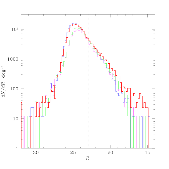
Figure 7: The differential $\log N-\log S$ distribution of detected galaxies in the central cluster field (red), and three background fields (blue, magenta, and green). The maximum in the $\log N-\log S$ histogram provides an estimate for a sensitivity limit in each field. The differences in the sensitivity limits primarily reflects differences in exposure. The vertical dotted line shows our adopted magnitude limit $R=22.9$, which is conservative and applicable for all cluster and background fields.

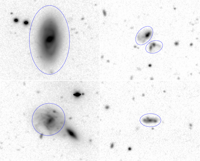
Figure 8: Examples of elliptical apertures used for flux measurements in bright spiral galaxies with complex morphology. Our source detection algorithm fails for such galaxies because it splits them into several objects. Therefore, their fluxes were re-measured in hand-set elliptical apertures.

3.3.3 Completeness limits

The difference in total accumulated exposure in different locations leads to the differences in the completeness limit. To simplify the joint analysis of the entire A133 dataset, we need to define a single completeness limit. We identify completeness for each field, using the peak location in the differential $\log N-\log S$ distributions. Examples are shown in Figure 7. The red histogram shows the source counts in the central cluster field, and the other three histograms show example source counts in the background fields. The maxima in the $\log N-\log S$ distributions are well defined, but broad, possibly because of substantial flux measurement uncertainties near the threshold sensitivity. To avoid this problem, we set a threshold for further analysis at $\approx 1$ magnitude brighter than the maximal point in the $\log N-\log S$ curves at $m\sim 24$. The adopted magnitude limits are $R=22.9$ and $V=22.6$. In the $R$-band, this limit corresponds to an absolute magnitude of $M_{R}=-14.1$ at the cluster distance. This is $\approx 5.4$ magnitudes below $M^{*}$ of the $R$-band field galaxy luminosity function (Lin et al., 1996).

3.4 Red sequence

Spectroscopic redshifts are unavailable for the majority of galaxies detected in the IMACS fields (Connor et al., 2018). Therefore, we need to subtract the statistical background, which corresponds to the contribution of foreground and background galaxies to the galaxy stellar mass functions, cluster light profile, etc. These contributions were measured in our offset background fields (see § 3 above). The surface number density contrast of the cluster members relative to the statistical background of galaxies with the same apparent magnitude is low, except for the central pointing (e.g., Figure 7). Therefore, we conservatively use additional selection criteria to remove galaxies unlikely to be associated with A133.

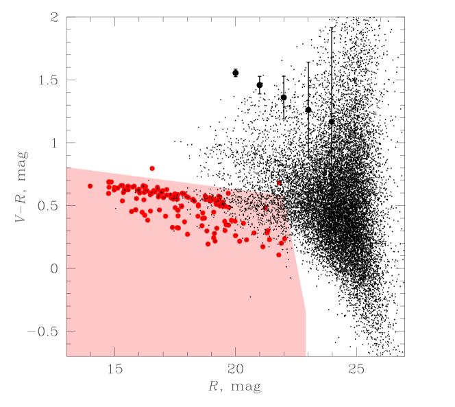
Figure 9: Color-magnitude diagram for galaxies in the central cluster field. The shaded region shows our selection criteria for A133 members. This region is limited by the $R$ and $V$ magnitude limits on the right, and by the color-magnitude cut on the top. Red points represent cluster galaxies with known spectroscopic redshifts over all cluster fields (Connor et al., 2018). The points with vertical errorbars indicate typical uncertainties of the V-R color.

Our selection is based on the cluster red-sequence method extensively used for studies and identification of galaxy clusters (e.g., Bower et al., 1992a, b; Gladders et al., 1998; López-Cruz et al., 2004; Koester et al., 2007; Valentinuzzi et al., 2011; Rykoff et al., 2014). The underlying idea is that red, passively evolving cluster members have similar colors and form a narrow sequence in the color-magnitude diagram. Some of the galaxies within the cluster, e.g. those with recent bursts of star formation, can be bluer than the red sequence (e.g., Connor et al., 2019a). However, there should be very few, if any, galaxies redder than the red sequence members because those members have the oldest stellar populations. The small number of objects above the red sequence are “special cases”, such as dust-covered AGNs, in which the stellar mass measurements based on optical luminosities are problematic. Empirically, these considerations are confirmed by the colors of the A133 members with spectroscopic redshifts (Figure 9).

For the A133 analysis, we used the $V-R$ color-magnitude diagram. This diagram for the central field (Figure 9) clearly shows the red sequence corresponding to the A133 redshift. We selected potential cluster members as the objects below or just above the cluster red sequence, $V-R<1.13-0.025R$, and brighter than the completeness limits for the $R$- and $V$-band images (recall that these are $R=22.9$ and $V=22.6$, see § 3.3.3). These criteria select a pink-shaded region in the color-magnitude diagram.

We emphasize again that these selection criteria are conservative. To improve the cluster contrast still further, we could have used a narrow color band around the red sequence, or additional selection criteria such as galaxy apparent sizes. However, we then would risk missing some of the cluster members with unusual properties. Since our main goal is the maximally complete census of the cluster stars, we use more inclusive selection criteria described above.

In addition to A133’s red sequence, the color-magnitude diagram seems to show a second sequence with redder colors, $V-R\approx 0.95$ at $R\approx 20$. We attribute it to the background cluster projected onto the core A133, for the following reasons. There is indeed a group of redder galaxies with smaller diameter in this region (Figure 2). The brightest of these redder galaxies, at RA=01:02:45.2 and Dec=$-$21:54:14, has a measured spectroscopic redshift, $z=0.293$. The location of that second red sequence is in excellent agreement with the red sequence of Z3146 ($z=0.2906$) measured by Kausch et al. (2007) in the same filters. Most of galaxies in this background cluster should be excluded by our color-magnitude selection of potential A133 members.

Selection of potential cluster members by means of the color-magnitude diagram concludes our preliminary data analysis steps. In what follows, we describe how stellar masses of individual galaxies were estimated from the optical luminosities, and how they were used to derive the stellar mass functions and the total stellar mass profiles within the cluster.

4 Results: Stellar mass function of the cluster members

4.1 Galaxy stellar mass estimates

Using the measured $R$-band magnitudes and $V-R$ colors, we estimated the stellar mass of each galaxy. The method is based on the stellar populations synthesis models from Bell et al. (2003). The first step is to convert the apparent magnitudes to the absolute magnitudes in $R$- and $V$- bands. We used the standard relation, $M=m-25-\log(D_{L}\,{\rm Mpc})-A-K(z)-EC$, where $D_{L}$ is the luminosity distance, $A$ is the interstellar extinction correction from Schlegel et al. (1998), $K(z)$ is the $K$-correction, and $EC$ is the evolutionary correction. The $K$-corrections were obtained from the “$K$-correction calculator” (Chilingarian et al., 2010; Chilingarian & Zolotukhin, 2012). The evolutionary correction $EC$ is adopted from Poggianti (1997) where it is provided for different galaxy types and a set of photometric bands. We used the $EC$ values averaged over galaxy types. We also note that the evolutionary correction, $EC=-0.08$, is small at the A133 redshift in both our filters. The described procedure is used to estimate $z=0$ absolute magnitude in the $R$ band and a de-redshifted $M_{V}-M_{R}$ color for each galaxy.

To obtain the stellar mass from these parameters, we convert the $R$-band absolute magnitude to the luminosity in Solar units using $M_{R,\odot}=4.42$ for the absolute $R$-band magnitude of the Sun (Binney & Merrifield, 1998). The luminosity is then converted to the stellar mass. This conversion is a function of the $M_{V}-M_{R}$ color. Using the Bell et al. (2003) fitting formulae for $M_{\star}/L_{R}$ as a function of $M_{B}-M_{V}$ and $M_{B}-M_{R}$, we obtain (in Solar units):

$$\lg(M_{\star}/L_{R})=-0.528+1.818(M_{V}-M_{R}).$$ (2)

The main uncertainty in the derived stellar masses is due to assumptions on the initial mass function of the stellar population which enter the population synthesis models. Note that the Bell et al. calibration used the “diet Salpeter” IMF model (see discussion in §2.4 of Kravtsov et al. 2018 regarding this choice of the IMF model and its effects on the stellar mass determination). In this work, we will use the “diet Salpeter” based masses. To convert to, e.g., the Chabrier (2003) IMF, our stellar masses should be scaled down by 0.1 dex.

4.2 Stellar mass functions of A133 galaxies

Before deriving the total cluster stellar mass as a function of radius, we need to explore how much light or stellar mass we may be missing below the completeness limits of our data. We address this question by analyzing the stellar mass functions of A133 galaxies.

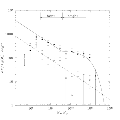
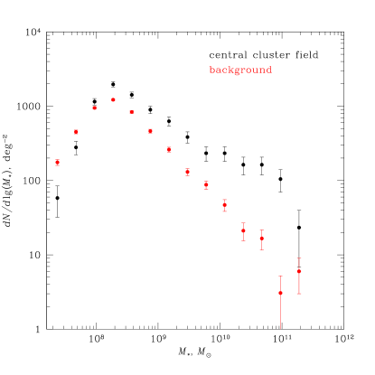
Figure 10: Stellar mass function for galaxies in the central and off-center cluster fields (filled and open circles, respectively), normalized to the area on the sky. The cluster BCG is excluded from this plot. The solid and dashed lines show the best-fit power-law$+$exponential and power-law models (see Eq. 3 and accompanying text). The right panel shows the raw data for the central field and the background, to illustrate that detection of the two-component structure of the stellar mass function is indeed robust. The data for the left panel of this figure is available at an online repository https://doi.org/10.5281/zenodo.3610482.

In Figure 10, we show the mass functions measured in the central and off-center cluster fields, normalized to the unit area on the sky. The background number density of galaxies has been measured using our off-cluster pointings and subtracted from these data. The observed mass functions show a roll-over below $M_{\star}\approx 2\times 10^{8}M_{\odot}$. To avoid incompleteness in our stellar mass measurements, we use only galaxies with $M_{\star}>3\times 10^{8}\,M_{\odot}$ in the further analysis. To account for the stellar mass potentially “lost” below this threshold, we estimate fractional correction factors using analytic fits to the mass function (see below).

Another prominent signature apparent from Figure 10 is a two-component structure of the mass function in the central pointing (filled circles in the figure). Above $\approx 4\times 10^{9}\,M_{\odot}$, it follows a Schechter-type (Schechter, 1976) function with an exponential cutoff around $M_{\star}\approx 10^{11}\,M_{\odot}$. At lower masses the stellar mass function steepens and its behavior is consistent with a power law down to our completeness limit. However, the mass function cannot be adequately fit with a single Schechter model over a broad mass range. The two-component form of the mass function in the central field is supported by comparison with the mass function in the off-center fields (open circles in Figure 10). This later mass function is consistent with a power law with the same slope as that for the faint end of the mass function near the cluster center. The existence of two separate components is also supported by the radial profile analysis in different mass ranges (see § 5.1 below). Following all these considerations, we modeled the central mass function separately above and below the “ankle” at $M_{\star}=4\times 10^{9}\,M_{\odot}$. Above this mass, we use a Schechter model:

$$\frac{dN}{d\lg M}=N_{0}\left(\frac{M}{M_{0}}\right)^{\alpha}\exp\left(-\frac{M}{M_{0}}\right)\,\mathpunct{\raisebox{2.15277pt}{,}}$$ (3)

where $N_{0},M_{0},\alpha$ are fitted parameters. In practice, $\alpha$ is unconstrained, given a small dynamical range in masses for the bright end of the mass function. Therefore, we fixed $\alpha=0$.

For the mass function in the off-center fields, we used a pure power law model (dashed line in Figure 10). The best-fit power law slope is $\alpha=-0.55\pm 0.11$. The analytic model of the central mass function in the $3\times 10^{8}\,M_{\odot}<M_{\star}<4\times 10^{9}\,M_{\odot}$ range is obtained by using a power law with the same fixed slope $\alpha_{0}=-0.55$ and a normalization chosen to match the Schechter fit (Eq. 3) for brighter galaxies at $M_{\star}=4\times 10^{9}\,M_{\odot}$. This fit is also shown by the solid line in Figure 10. It provides a good description to the data.

We note that the total mass for a power law mass function with a slope of $\alpha=-0.55$ converges at the faint end. Therefore, there is no evidence that we may be missing a significant population of dwarf galaxies which is important for the total stellar mass budget in the cluster. We also note that if there were a significant population of undetectable galaxies, especially in the cluster center, it would contribute to the extended diffuse light envelope, which we analyze and account for separately (§ 5.2). In the further analysis, we assume that the power law behavior continues to extremely low masses, and we apply the corresponding “incompleteness” correction of $\times 1.45$ for the total mass of galaxies with $M_{\star}<4\times 10^{9}\,M_{\odot}$. The galaxies with $M_{\star}>4\times 10^{9}\,M_{\odot}$ are counted and modeled separately (see below), and they require no incompleteness corrections.

5 Results: Stellar Mass Profile

Using the results for the stellar mass function of the cluster members, we proceed to a derivation of the stellar mass profile in the cluster. Our general approach is to directly count the contribution of each galaxy with estimated mass $M_{\star}>3\times 10^{8}\,M_{\odot}$, and then correct the total for incompleteness at the faint end of the mass function (see above). We derived the stellar mass profile of the brightest cluster galaxy separately, tracing the wings of its light profile to $R\approx 200\,$ kpc. The derived projected profiles of both the BCG and other cluster galaxies are fit to analytic functions defined in 3D, and so deprojection is straightforward.

5.1 Contribution from Cluster Member Galaxies

To determine the stellar mass profile for non-central galaxies, we computed the surface mass density in radial bins of equal log-width, centered on the BCG. Since there are indications that the mass function of the cluster members has two distinct components, we computed the surface mass density separately in two mass intervals, $3\times 10^{8}<M_{\star}<4\times 10^{9}\,M_{\odot}$ and $M_{\star}>4\times 10^{9}\,M_{\odot}$. The lower boundary corresponds to the estimated completeness limit, and the middle point corresponds to the “ankle” in the mass function (Figure 10). In the same mass ranges, we computed the contribution of background galaxies to the surface mass density, using the data from eight background fields. This statistical background was subtracted from the projected cluster mass profiles.

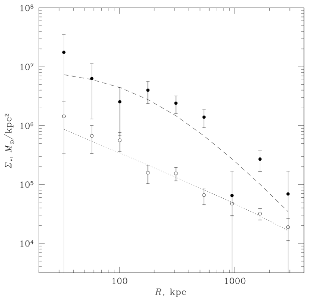
Figure 11: The projected cluster stellar mass profile, derived for galaxies with individual masses in the ranges $(3-40)\times 10^{8}\,M_{\odot}$ (open circles) and $(40-2500)\times 10^{8}\,M_{\odot}$ (filled circles). The lines show the best-fit model (see Eq. 4 and accompanying text). The difference in shape in the two mass profiles is insensitive to the exact choice of the boundary between “faint” and “bright” galaxies.

The results are shown in Figure 11. Indeed, the figure shows different radial profiles for the massive and lower-mass galaxies, which reflects a well known radial dependence of the dwarf-to-giant galaxy fraction in clusters (e.g., Smith et al., 1997; Barkhouse et al., 2009). The lower-mass galaxies have a power-law type profile with a projected slope of $-0.77\pm 0.20$. The profile for massive galaxies has a flat core out to $R\approx 400-500$ kpc (nearly $0.5\,r_{500c}$). Beyond this radius, the profile steepens. While the measured profiles are quite noisy, there is still a tentative detection of the cluster signal in both components out to at least $\approx 2$ Mpc, beyond the estimated $r_{200c}$ radius.

To deproject these profiles, we fit them using a projected analytic function defined in 3D. Specifically, we used a “Nuker” density profile (cf., Lauer et al., 1995; Kravtsov et al., 1998), which can be viewed as a generalized version of the Navarro-Frenk-White (NFW Navarro et al., 1997) profile:

$$\rho(x)=\frac{{\rho}_{0}}{x^{\alpha}(1+x^{\gamma})^{(\beta-\alpha)/\gamma}}\,\mathpunct{\raisebox{2.15277pt}{,}}$$ (4)

where $x=r/{r_{s}}$, $r_{s}$ is the scale radius, and $\rho_{0}$ is the density scale. The profile inner slope is controlled by $\alpha$, $\beta$ controls the outer slope, and $\gamma$ determines how fast the profile slope changes around $r=r_{s}$. This model has been numerically integrated along the line of sight and fit to the data.

Since our measured profiles are noisy, we did not fit all parameters independently. For massive galaxies, we fitted $\rho_{0}$ and $r_{s}$ and fixed the inner slope at $\alpha=0$, the outer slope at $\beta=3$ as expected in the NFW models, and also fixed $\gamma=1$. For the low-mass galaxies, we used a power-law limit of Eq. (4) by fixing $r_{s}$ at a high value. The best-fit projected profiles are shown as dashed lines in Figure 11.

The 3D radial profile of the stellar mass in the cluster can be obtained straightforwardly by integrating the best-fit density profile of Eq. 4. To estimate the statistical uncertainties of the derived mass profiles, we used the Monte-Carlo method described in Vikhlinin et al. (2006). We generated multiple realizations of the data by scattering the profile data points according to their statistical uncertainties, re-fit the models, re-derived the mass profiles, and computed the scatter of mass values at each radius, averaged over the realizations. The resulting stellar mass profiles with uncertainties are shown in Figure 15 below.

5.2 Brightest Cluster Galaxy

The contribution of the brightest cluster galaxy to the stellar mass budget was considered separately because this galaxy is bright and very extended, and therefore cannot be treated as a point mass. We start by extracting the BCG light profiles in the $R$, $V$, and $I$ filters. Unlike the analysis of non-central galaxies, we used the global background subtraction (§ 3.2) because the locally estimated background subtracts the extended wings of the BCG profile. Unfortunately, the global background subtraction is less accurate, leading to increased uncertainties of the BCG profile at large radii. To estimate the level of these uncertainties, we extracted $R$, $V$, and $I$-band light profiles around three representative locations in each of the background and cluster off-center pointings not contaminated by bright stars.

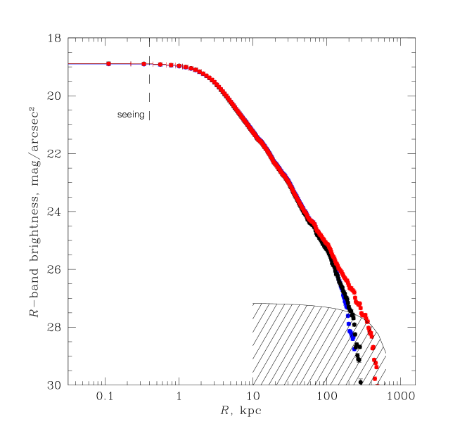
Figure 12: The raw BCG light profile in three filters $R$ (red), $V$ (blue), and $I$ (black). For clarity, the $V$ and $I$-band profiles were renormalized to match the $R$-band profile at small radii. The shaded region shows a level of estimated background uncertainties as a function of radius (see text).

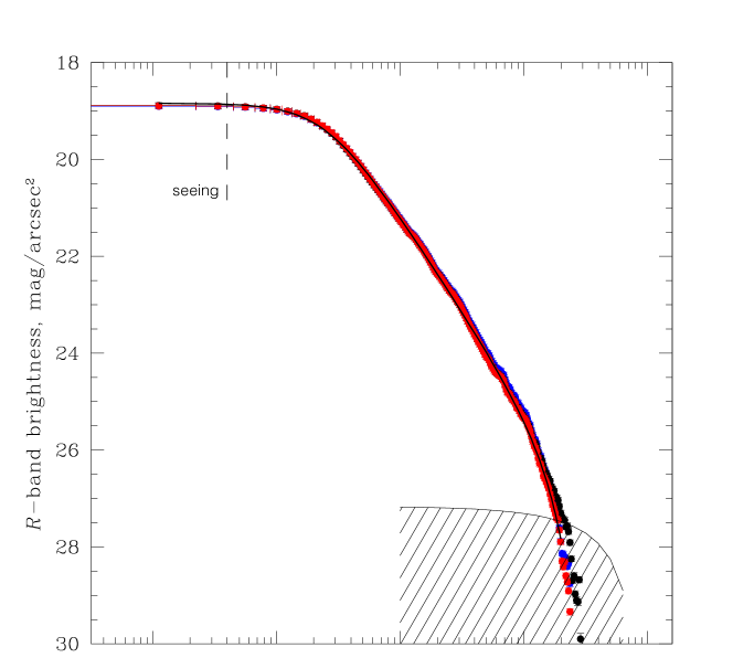
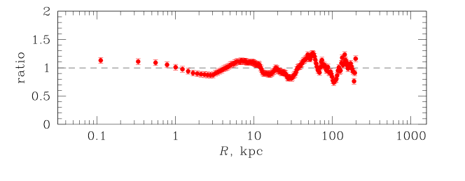
Figure 13: Same as Figure 12, but with the uniform background correction applied to the $R$-band data (see text). The black solid line shows the best-fit model (see Eq. 5 and accompanying text). The bottom panel shows model residuals.

The resulting light profile of the BCG in $R$, $V$, and $I$ filters is shown in Figure 12. We have applied uniform offsets $-0.66$ and $+0.64$ magnitudes per arcsec² to the $V$ and $I$-band profiles, respectively, to match the $R$-band brightness at small radii. Note that this BCG $V-R$ color exactly corresponds to the red sequence location for the brightest cluster members (Figure9). The level of estimated background subtraction uncertainties in the $R$-band is shown by a hatched region. The observed light profiles in all three filters follow one another very precisely out to $r\approx 150\,$kpc where the $R$-band brightness reaches a 26 mag arcsec^-2 level. Outside this radius, the $V$ and $I$-band profiles continue to follow one another, while the $R$-band brightness shows a significant positive deviation. A brightness excess appearing only in the $R$ band is not expected for normal stellar population spectra, where systematic trends run from $V$ through $R$ to $I$. Therefore, a more likely cause of the observed $R$-band excess is inaccuracies in the global background subtraction at these low surface brightness limits. We find that an additional, uniform, background correction of 26.9 mag arcsec^-2 in the $R$-band is sufficient to completely match the data in all three filters (Figure 13). This is only 60% higher than the typical observed level of background variations at $R=200\,$kpc, and so such corrections are very likely. We use the $R$-band profile with this additional background correction in the analysis below. However, we recognize that the measurements become extremely sensitive to the background subtraction at $R>200\,$kpc, and therefore we restrict the mass measurements to within this radius. In Figure 14, we show a zoom-in on the composite $R$-band image near the BCG location. The 200 kpc radius is shown by the red circle. The wings of the BCG brightness in the NE and SW directions can indeed be traced visually very close to this radius.

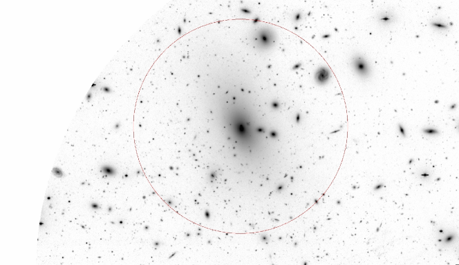
Figure 14: Central cluster region around the BCG galaxy in the R-band. Red circle shows a region of $200$ kpc radius where we measured the BCG light profile. The wings of the BCG brightness in the NE and SW directions can indeed be traced visually very close to this radius.

To reconstruct the 3D stellar mass profile of the BCG, we use an approach similar to that in §5.1. We fit the observed light profile with a projected density model defined in 3D and then integrate that model as a function of radius. In this case, we used a modified $\beta$-model (c.f. Vikhlinin et al., 2006):

$$\rho(r)=\frac{{\rho}_{0}}{\left(1+(r/r_{c})^{2}\right)^{3\beta}}\frac{1}{\left(1+(r/r_{s})^{\gamma}\right)^{\epsilon/\gamma}}\,\mathpunct{\raisebox{2.15277pt}{,}}$$ (5)

where ${\rho}_{0},r_{c},r_{s},\beta,\gamma,\epsilon$ are fitted parameters. This model describes a flattening at small radii ($r\lesssim r_{c}$), a transition to a power law behavior at $r>r_{c}$, and a further change of the profile slope at large radii, $r\gtrsim r_{s}$. The best-fit model is shown by the solid black line in Figure 13 and provides an excellent fit to the data. Its best-fit parameters are $\rho_{0}=24.1$ mag arcsec^-2 kpc^-1, $r_{c}=2.5$ kpc, $r_{s}=245.1$ kpc, $\beta=0.42$, $\gamma=2.3$, $\epsilon=0.76$. We use this model to compute the $R$-band luminosity of the BCG as a function of 3D radius.

To convert this luminosity to the stellar mass, we use the mass-to-light ratio from Bell et al. (2003), just like we did for the other cluster members. There is only a small change in the observed color with radius: $V-R=0.66$ at the BCG center, dropping to $V-R=0.56$ at $r=50\,$kpc, beyond which the contribution of systematic background uncertainties (see above) makes color gradient measurements unreliable. Note that such color gradients are quite common in the BCG and the intracluster light (DeMaio et al., 2018). The corresponding change in the $M/L$ ratio, from $3.9\,M_{\odot}/L_{\odot}$ in the center to $2.6\,M_{\odot}/L_{\odot}$ at 50 kpc, was included in the conversion of the observed light profile to stellar mass. If, instead, one uses a fixed $V-R$ color measured at the center, the BCG stellar mass within 200 kpc is overestimated by 59%.

Finally, we note that the formal statistical uncertainties of the BCG light profile within 200 kpc are very small. The mass uncertainties should be completely dominated by those in the $M/L$ ratio (e.g., those related to the color gradient or assumptions on the IMF in the the stellar population synthesis models, c.f. § 4.1).

5.3 Total stellar mass profile

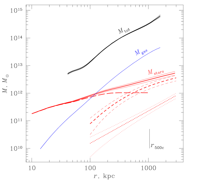
Figure 15: 3D profile of enclosed stellar mass of the three stellar components: the red dotted line is for low-mass cluster galaxies of $M_{\star}=(3-40)\times 10^{8}\,M_{\odot}$, the red dashed line shows high-mass cluster galaxies of $M_{\star}=(40-2500)\times 10^{8}\,M_{\odot}$, and the red long dashed line represents the BCG. The solid red line shows the summed profile of the three stellar components of the cluster. Blue is the X-ray estimated mass profile of gas and black line is the total mass profile derived from Chandra X-ray data using hydrostatic equilibrium assumption (Vikhlinin et al. in preparation). Short vertical black line indicates the $r_{500c}$ radius.

In Figure 15, we show the total reconstructed stellar mass profile within A133 and its individual components discussed above (estimates of $M_{\star}$ within different $r$ are also presented in Table 1). For comparison, we also show the profile of the hot gas and of the total mass reconstructed from the X-ray data (Vikhlinin et al., in preparation, see also Vikhlinin et al., 2006). Several points about these profiles are noteworthy.

The central cluster galaxy contributes a large fraction of the total stellar mass. Its integrated mass within 200 kpc is approximately 50% of the rest of cluster galaxies within 1 Mpc ($\approx r_{500c}$), or $\sim 25\%$ at $r\approx 3$ Mpc (well outside of $r_{200c}$). The BCG dominates the total baryon mass, including hot gas, in the central $\approx 100$ kpc. The hot gas within this radius shows a spike in metallicity (see Figure 3 in Vikhlinin et al., 2005), likely reflecting extra enrichment due to stellar mass loss and supernovae within the BCG.

Non-central galaxies approximately follow the distribution of total mass in the radial range $\approx(0.1-1)\,r_{500c}$ where both the X-ray and optical measurements are most reliable. This is in line with a number of earlier studies for different clusters (e.g., Andreon, 2015; Palmese et al., 2016).

Small-mass galaxies of $M_{\star}<4\times 10^{9}\,M_{\odot}$ contribute a minor fraction of the total stellar mass even at large radii. At $r=3\,$Mpc, their contribution is $\approx 13\%$ and it is even lower at smaller radii. The majority of the cluster stellar mass is contributed by bright galaxies and the BCG. Nevertheless, the radial distribution of these faint galaxies is quite distinct from the radial distribution of brighter galaxies (see § 5.1 above). Namely, the radial distribution of stellar mass of faint galaxies is well described by a single power law profile, $\rho(r)\propto r^{-1.77\pm 0.20}$. We discuss possible interpretations of this fact in Section 6 below.

Table 1: Stellar mass measurements in Abell 133

$r/r_{500c}$	$r$, kpc	$M_{\textrm{BCG}}$	$M_{\textrm{bright}}$	$M_{\textrm{faint}}$	$M_{\textrm{stars}}$
0.1	105	$7.4$	$0.87\pm 0.49$	$0.16\pm 0.11$	$8.4\pm 0.5$
0.2	262	$10.2$	$4.1\pm 1.4$	$0.47\pm 0.21$	$14.8\pm 1.4$
0.5	524	$10.3$	$9.7\pm 2.5$	$1.06\pm 0.34$	$21.1\pm 2.5$
1.0	1048	$10.3$	$18.4\pm 4.2$	$2.4\pm 0.6$	$31.1\pm 4.2$
1.5	1572	$10.3$	$24.6\pm 5.5$	$3.8\pm 0.8$	$38.7\pm 5.6$
2.5	2620	$10.3$	$33.4\pm 7.6$	$7.0\pm 1.5$	$50.7\pm 7.8$

Note. — All masses are in units of $10^{11}\,M_{\odot}$ and computed for our default cosmology. The last column gives the total of the three components — the BCG, bright galaxies, and faint galaxies.

Finally, we note that at $r=r_{500c}$ and beyond, the stellar mass is a small fraction of the total baryonic mass (i.e., gas + stars), $\approx 11\%$. This is consistent with the values previously reported in the literature (e.g., Gonzalez et al., 2013; Kravtsov et al., 2018). Therefore, despite using a much deeper data and an ability to trace the BCG light profile to larger radii, we have not uncovered a major reservoir of cluster baryons associated with cluster galaxies. To substantially increase the fraction of stellar mass in the cluster baryon budget requires drastic revisions of the $M/L$ ratio values from stellar population synthesis. Such revisions are not supported by detailed modeling of the galaxy spectra (van Dokkum et al., 2017). We will present a detailed analysis of the matter components in A133, including dark matter and hot intracluster gas, in a subsequent paper.

6 Discussion of the radial dependence of galaxy stellar mass function

One of the key results of this paper is the upturn of the stellar mass function of satellite galaxies in A133 at $M_{\star}\lesssim 4\times 10^{8}\,M_{\odot}$. The best fit slope $\alpha$ of the power law in this dwarf galaxy regime is comparable with recent measurements of the faint-end slope of the stellar mass function of field galaxies of $-0.5\pm 0.05$ at $z=0.1$ (see, e.g., Wright et al., 2017, and references therein) and at higher redshifts (Wright et al., 2018; Papovich et al., 2018).

The existence of the upturn in the luminosity function in clusters and the value of the faint-end slope have been a subject of a long debate in the literature (e.g., Driver et al., 1994; Smith et al., 1997; Barkhouse et al., 2007; Rines & Geller, 2008; Harsono & De Propris, 2009; Agulli et al., 2014), which may be due to real diversity of the luminosity functions in clusters (e.g., Moretti et al., 2015) and, partly, due to degeneracy among model parameters in double-Schechter fits to LF. Nevertheless, the overall shape of the stellar mass function and its slope in the dwarf galaxy regime are qualitatively consistent with the form of $R$-band luminosity function measured in several nearby clusters (Smith et al., 1997) and groups (Zabludoff & Mulchaey, 2000). In addition, recent systematic study of luminosity function of galaxies in the SDSS groups and clusters by Lan et al. (2016) reported a Schechter$+$power law shape qualitatively similar to that we measured for A133.

Another intriguing result of this study is that the shape of the stellar mass function changes with radius. This is reflected in the difference in the radial distribution of low- and high-luminosity galaxies (Figure 11). It is likely that this difference is related to the decrease of the “dwarf-to-giant ratio” towards cluster center that was previously reported in several clusters (e.g., Smith et al., 1997; Sánchez-Janssen et al., 2008; Barkhouse et al., 2009).

Cosmological simulations of structure formation in the $\Lambda$CDM model predict that mass and radial distributions of host halos of satellite galaxies are nearly self-similar (e.g., Kravtsov et al., 2004; Nagai & Kravtsov, 2005; van den Bosch & Jiang, 2016; Hellwing et al., 2016) throughout most of cluster volume. Recent study by Han et al. (2018) indicates that this self-similarity is broken at $r/R_{200}\lesssim 0.2$, where massive halos have steeper radial distribution resulting in a smaller dwarf-to-giant halo ratio at these radii. The difference is due to dynamical friction experienced by massive halos, which brings them closer to the cluster center.

However, the difference in the radial distribution of dwarf and luminous galaxies in A133 persists out to $r\sim R_{200}$ and thus unlikely to be due solely to dynamical friction. The significant difference in radial and stellar mass distribution of galaxies of different mass is likely to be yet another manifestation of the break of self-similarity of galaxy properties due to star formation and feedback processes accompanying galaxy formation (see Somerville & Davé, 2015; Naab & Ostriker, 2017, for reviews).

One of the potential consequences of feedback in dwarf galaxies is flattening of their central dark matter density profiles (Navarro et al., 1996; Mashchenko et al., 2008; Pontzen & Governato, 2012) – the effect that is most efficient for galaxies of stellar mass $M_{\star}\sim 10^{9}-10^{10}\,M_{\odot}$ (e.g., see Section 3.1.1 in Bullock & Boylan-Kolchin, 2017, for a review). Another effect of galaxy formation that breaks self-similarity is that gas mass fractions are, on average, much larger in dwarf galaxies compared to the giant galaxies. Gas rich dwarfs suffer both tidal stripping and ram pressure stripping of halo and interstellar gas. The latter, if sufficiently fast, can lead to rapid decrease of the gravitational potential depth in the inner regions and significant enhancement of tidal stripping of the stellar component in dwarf galaxies relative to massive ones (Safarzadeh & Scannapieco, 2017).

Interestingly, the radial profile of dwarf galaxies we measured in A133 can be described by a power law with a slope close to that expected for the distribution of objects on their first infall. Indeed, the spherical infall model predicts that before shell crossing the density profile of matter is $\rho\propto r^{-\gamma}$ with $\gamma\approx 1.5$, while we derive $\rho_{\mathrm{3D}}\propto r^{-1.77\pm 0.2}$ for faint galaxies (§5.1).

Notably, a similar power law radial distribution of blue galaxies was measured in the SDSS (Baxter et al., 2017) and the DES clusters (Shin et al., 2018). Given the expectation for the power law profile of infalling population of matter and galaxies, the most straightforward interpretation of this result is that galaxies do not remain blue much beyond the first pericenter passage and that the population of blue galaxies is thus dominated by infalling galaxies on their first approach to the pericenter, as was previously suggested for dwarf galaxy populations in Fornax (Drinkwater et al., 2001) and Virgo (Conselice et al., 2001) clusters. Physically, this can happen if star formation of galaxies is decreased and their color reddens on the time scale comparable to the cluster crossing time. The power law distribution of dwarf galaxies we find in A133 can have a similar origin, at least partly, although the reasons for the disappearance of dwarf galaxies from the sample after the pericenter passage may be different.

Galaxies can suffer significant morphological transformations and mass loss due to tidal forces (e.g., Moore et al., 1999) that peak strongly around the orbital pericenter. For a given orbit and strength of the tidal force, stellar systems embedded in a halo with flattened central dark matter density profile would experience stronger mass loss and can experience significant increase in the half-mass radius of the stellar distribution (Errani et al., 2015, 2017). The latter will lead to a significant decrease of the galaxy stellar surface density and surface brightness, potentially bringing it below detection limit of our observations. Thus, feedback that is expected to flatten dark matter distribution predominantly in the centers of dwarf galaxies of $M_{\star}\sim 10^{9}-10^{10}\,M_{\odot}$ may affect dwarf and luminous galaxies very differently, thereby breaking the self-similarity of gravitational collapse. Indeed, Weinmann et al. (2011) compare results of the semi-analytic models used with cosmological simulations of clusters that match observed dwarf-to-giant galaxy ratios in Virgo, Fornax, Coma, and Perseus clusters and conclude that the tidal disruption of dwarf galaxies needs to be enhanced in the models. Observations also show indications that low surface brightness galaxies suffer significant tidal stripping and disruption in the central regions of clusters (e.g., Wittmann et al., 2017).

Another interesting fact is that in group-scale halos the dwarf-to-giant ratio appears to be enhanced compared to the field (Zabludoff & Mulchaey, 2000) – the trend opposite to that found in massive clusters, and which is reflected in the systematic change of the shape of the luminosity function from rich clusters to groups (Lan et al., 2016). This trend can be understood as a net result of two opposing trends: the increased efficiency of tidal disruption of dwarf galaxies in massive clusters due to stronger tides and larger rate of disruption of massive galaxies in groups due to more efficient dynamical friction.

7 Summary and Conclusions

This paper presents the analysis of deep optical imaging observations of the galaxy cluster Abell 133 with Magellan/IMACS. The summary of our main results is as follows:

• The stellar mass function of cluster member galaxies is reliably measured down to a mass limit of $M_{\star}=3\times 10^{8}\,M_{\odot}$ ($\approx 0.1$ of the LMC stellar mass). The mass function shows a clear two-component structure with an excess of $M_{\star}<4\times 10^{9}\,M_{\odot}$ galaxies over an extrapolation of the Schechter fit from higher masses. There is a background cluster ($z=0.29$) projected on the center of A133, but based on the spatial distribution of faint galaxies we confirm that the low-mass component is associated with A133 itself.

• Interestingly, the radial profile of dwarf galaxies ($M_{\star}<4\times 10^{8}\,M_{\odot}$) we measured in A133 can be described by a power law with a slope of $-1.77\pm 0.2$. This is close to the power law radial distribution with the slope of $\approx-1.5$ expected for objects on their first infall in the spherical infall model of cluster formation. This similarity may indicate that dwarf galaxies are disrupted efficiently in clusters and that most of them do not survive for more than a single orbit. However, additional observational measurements and more detailed modelling is required to test this conjecture.

• We have measured an extended halo of the brightest cluster galaxy to $\sim 200$ kpc. Its profile is fully within the range of BCG envelopes measured for other low-z clusters (e.g., Kravtsov et al., 2018). Including the outer envelope, the BCG contributes $33\%$ of the cluster stellar mass within $r_{500c}$, also in the range of previously observed values (Gonzalez et al., 2000; Kravtsov et al., 2018; Zhang et al., 2019; Kluge et al., 2019; DeMaio et al., 2020).

• The total stellar mass has been measured in a range of radii out to $\approx 2.5\,$Mpc with formal statistical uncertainties of $<15\%$. The dominant source of systematic uncertainty is the stellar mass-to-light ratio. We have used the $V-R$ color dependence of $M/L$ from Bell et al. (2003) computed using population synthesis models and corrected to a “diet Salpeter” stellar initial mass function. For comparison, the $M/L$ values for the Chabrier (2003) IMF would already be $\sim 25\%$ lower. Detailed studies of the impact of the $M/L$ assumptions on the stellar mass measurements in A133 are beyond the scope of this paper.

Appendix A wvdecomp overview and empirical noise maps

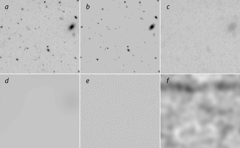
Figure 16: Steps in making the spatially-nouniform noise maps for source detection. The flat-fielded, background-subtracted image (panel a) and a first-iteration noise map (see text) serve as inputs to the initial run of wvdecomp. The output (panel b) is detected structures on spatial scales $\sim 0.2^{\prime\prime}-7^{\prime\prime}$; this map is 0 outside of the “islands” defined by detected structures. Panel c is the source-cleaned image, obtained as a difference of maps in panels a and b. Panel d is the convolution of data in panel c with a Gaussian of $\sigma=25^{\prime\prime}$; this served as the local background map (see § 3.2). Panel e is the convolution of data in panel c with the wvdecomp kernel on the $0.4^{\prime\prime}$ spatial scale. It is an estimate of pixel-to-pixel noise in the original image, modulo a renormalization factor of 0.20066. Panel f is the final noise map obtained by smoothing the square of the data in panel e with a Gaussian kernel with $\sigma=3^{\prime\prime}$.

wvdecomp is the wavelet-based algorithm for finding stastically significant structures in astronomical images and separating them into a range of spatial scales of interest. For full reference, see Vikhlinin et al. (1998). Here we review the outputs produced by wvdecomp and explain how these were used to compute spatially-dependent noise maps (§ 3.3.1).

The procedure is illustrated in Figure 16. The first run of wvdecomp over the input flat-fielded and background-subtracted image (shown in panel a) uses an approximate noise map, computed from the mean rms deviations over the full image area and only corrected for exposure variations. One of the outputs of wvdecomp is the image containing identified statistically significant structures (in this case, on spatial scales $\sim 0.2^{\prime\prime}-7^{\prime\prime}$; see panel b). An equivalent image at the end of this procedure can be used to identify sources simply by finding local maxima in this wvdecomp output, as shown in Figure 3 above. This image can also be used to identify “islands” of significant signal around each detected sources. Such islands are useful for selecting image subsections for more detailed modeling, and for masking out unrelated sources. Identification of the islands is straightforward for isolated sources. In case of the overlapping sources, a version of the “water fill” algorithm can be used (He et al., 2013). A similar algorithm is used for source de-blending in SExtrator (Bertin & Arnouts, 1996).

Here, we use the wvdecomp output to compute the source-cleaned image which retains all of the noise (panel c). A convolution of this source-free image with a wide Gaussian (panel d) gives an estimate of the local background (c.f. § 3.2). Note a slight enhancement of the estimated background at the position of a brighter ellptical galaxy near a top-right corner of the image. This enhancement is insignificant in this case, but becomes a problem for the brightest galaxies and the cluster BCG, in which cases we used the global background (§ 3.3.2). A convolution of the same source-free image with the wvdecomp’s wavelet kernel, which is then squared, appropriately renormalized, and smoothed with a $\sigma=3^{\prime\prime}$ Gaussian, provides an estimate of the spatially-variable noise (panel f). This map serves as an input to the final run of wvdecomp leading to source detections (see Figure 3 for comparison).

Appendix B Comparison of stellar masses derived from Magellan and DES data

In order to ensure the reliability of our measured galaxy masses we compared them with masses derived from photometric data of the Dark Energy Survey (Data release 1) (DES Collaboration, 2018). We selected the DES sources around the Abell 133 BCG position and matched with our catalogue in the central cluster field. Our sources belong to the red sequence and considered to be cluster galaxies. The DES did not observe in $V$; therefore we used $g$ filter instead. We converted DES $g$ and $r$ magnitudes into sdss magnitudes, applied the $K$-correction, transformed magnitudes to luminosities and then to masses using Bell et al. (2003) expressions. Derived DES masses and our measured masses from the Magellan data are plotted in the Figure 17. Outliers with overestimated DES masses are located near the BCG and a bright galaxy, or parts of double sources.

We have repeated the entire analysis chain presented in this paper using DES catalogs. The DES data are shallower, but cover the entire cluster region. The stellar mass functions and the mass profiles derived from DES are fully consistent with our measurements (Figure 18). We could not use DES data for fitting the outer envelope of the BCG because of the over-subtraction of the background in the publically available DES images. Using DES results for non-central galaxies and our BCG profile, we obtain the total stellar mass $M_{\star}=(20.1\pm 3.7)\times 10^{11}\,M_{\odot}$, $(31.6\pm 5.8)\times 10^{11}\,M_{\odot}$, and $(40.8\pm 6.4)\times 10^{11}\,M_{\odot}$ at $r=0.5$, $1$, and $1.5\,r_{500c}$, respectively, in good agreement with our values reported in Table 1.

Figure 17: Comparison of galaxy stellar mass measurements from this study and those based on the DES photometries. The black dotted line indicated our adapted lower mass limit of $3\times 10^{8}\,M_{\odot}$ (§ 4).

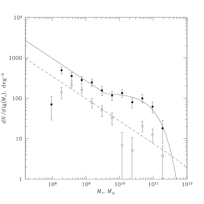
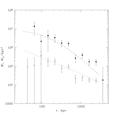
Figure 18: Stellar mass functions and the projected mass profiles for non-central galaxies derived from the DES data. The figures are equivalent to Figure 10 and 11. The lines show analytical fits to our Magellan data. Completeness of the mass function is reached at a higher threshold compared to Magellan data, so we used the mass range $M_{\star}=(6-40)\times 10^{8}\,M_{\odot}$ for the “faint galaxies” profile shown in the right panel. A somewhat lower normalization of this profile relative to the Magellan fit is fully consistent with the difference in the incompleteness corrections (cf. §4.2), 1.74 vs. 1.45 for the $M_{\star}=(3-40)\times 10^{8}\,M_{\odot}$ mass range we used for Magellan data.

References

- Agulli et al. (2014) Agulli, I., Aguerri, J. A. L., Sánchez-Janssen, R., et al. 2014, MNRAS, 444, L34, doi: 10.1093/mnrasl/slu108
- Allen et al. (2011) Allen, S. W., Evrard, A. E., & Mantz, A. B. 2011, ARA&A, 49, 409, doi: 10.1146/annurev-astro-081710-102514
- Andreon (2015) Andreon, S. 2015, A&A, 575, A108, doi: 10.1051/0004-6361/201425122
- Bahé et al. (2017) Bahé, Y. M., Barnes, D. J., Dalla Vecchia, C., et al. 2017, MNRAS, 470, 4186, doi: 10.1093/mnras/stx1403
- Barkhouse et al. (2007) Barkhouse, W. A., Yee, H. K. C., & López-Cruz, O. 2007, ApJ, 671, 1471, doi: 10.1086/523257
- Barkhouse et al. (2009) —. 2009, ApJ, 703, 2024, doi: 10.1088/0004-637X/703/2/2024
- Barnes et al. (2017) Barnes, D. J., Kay, S. T., Bahé, Y. M., et al. 2017, MNRAS, 471, 1088, doi: 10.1093/mnras/stx1647
- Battaglia et al. (2013) Battaglia, N., Bond, J. R., Pfrommer, C., & Sievers, J. L. 2013, ApJ, 777, 123, doi: 10.1088/0004-637X/777/2/123
- Baxter et al. (2017) Baxter, E., Chang, C., Jain, B., et al. 2017, ApJ, 841, 18, doi: 10.3847/1538-4357/aa6ff0
- Bell et al. (2003) Bell, E. F., McIntosh, D. H., Katz, N., & Weinberg, M. D. 2003, ApJS, 149, 289, doi: 10.1086/378847
- Bellstedt et al. (2018) Bellstedt, S., Forbes, D. A., Romanowsky, A. J., et al. 2018, MNRAS, 476, 4543, doi: 10.1093/mnras/sty456
- Bennett et al. (2014) Bennett, C. L., Larson, D., Weiland, J. L., & Hinshaw, G. 2014, ApJ, 794, 135, doi: 10.1088/0004-637X/794/2/135
- Bertin & Arnouts (1996) Bertin, E., & Arnouts, S. 1996, A&AS, 117, 393, doi: 10.1051/aas:1996164
- Binney & Merrifield (1998) Binney, J., & Merrifield, M. 1998, Galactic Astronomy
- Bower et al. (1992a) Bower, R. G., Lucey, J. R., & Ellis, R. S. 1992a, MNRAS, 254, 601, doi: 10.1093/mnras/254.4.601
- Bower et al. (1992b) —. 1992b, MNRAS, 254, 589, doi: 10.1093/mnras/254.4.589
- Budzynski et al. (2014) Budzynski, J. M., Koposov, S. E., McCarthy, I. G., & Belokurov, V. 2014, MNRAS, 437, 1362, doi: 10.1093/mnras/stt1965
- Budzynski et al. (2012) Budzynski, J. M., Koposov, S. E., McCarthy, I. G., McGee, S. L., & Belokurov, V. 2012, MNRAS, 423, 104, doi: 10.1111/j.1365-2966.2012.20663.x
- Bullock & Boylan-Kolchin (2017) Bullock, J. S., & Boylan-Kolchin, M. 2017, ARA&A, 55, 343, doi: 10.1146/annurev-astro-091916-055313
- Busch & White (2017) Busch, P., & White, S. D. M. 2017, MNRAS, 470, 4767, doi: 10.1093/mnras/stx1584
- Chabrier (2003) Chabrier, G. 2003, PASP, 115, 763, doi: 10.1086/376392
- Chilingarian et al. (2010) Chilingarian, I. V., Melchior, A.-L., & Zolotukhin, I. Y. 2010, MNRAS, 405, 1409, doi: 10.1111/j.1365-2966.2010.16506.x
- Chilingarian & Zolotukhin (2012) Chilingarian, I. V., & Zolotukhin, I. Y. 2012, MNRAS, 419, 1727, doi: 10.1111/j.1365-2966.2011.19837.x
- Connor et al. (2019a) Connor, T., Kelson, D. D., Donahue, M., & Moustakas, J. 2019a, ApJ, 875, 16, doi: 10.3847/1538-4357/ab0d84
- Connor et al. (2019b) Connor, T., Zahedy, F. S., Chen, H.-W., et al. 2019b, ApJ, 884, L20, doi: 10.3847/2041-8213/ab45f5
- Connor et al. (2018) Connor, T., Kelson, D. D., Mulchaey, J., et al. 2018, ApJ, 867, 25, doi: 10.3847/1538-4357/aae38b
- Conselice et al. (2001) Conselice, C. J., Gallagher, John S., I., & Wyse, R. F. G. 2001, ApJ, 559, 791, doi: 10.1086/322373
- Cui et al. (2018) Cui, W., Knebe, A., Yepes, G., et al. 2018, MNRAS, 480, 2898, doi: 10.1093/mnras/sty2111
- DeMaio et al. (2018) DeMaio, T., Gonzalez, A. H., Zabludoff, A., et al. 2018, MNRAS, 474, 3009, doi: 10.1093/mnras/stx2946
- DeMaio et al. (2020) —. 2020, MNRAS, 491, 3751, doi: 10.1093/mnras/stz3236
- DES Collaboration (2018) DES Collaboration. 2018, ApJS, 239, 18, doi: 10.3847/1538-4365/aae9f0
- Diemer & Kravtsov (2014) Diemer, B., & Kravtsov, A. V. 2014, ApJ, 789, 1, doi: 10.1088/0004-637X/789/1/1
- Dressler et al. (2011) Dressler, A., Bigelow, B., Hare, T., et al. 2011, PASP, 123, 288, doi: 10.1086/658908
- Drinkwater et al. (2001) Drinkwater, M. J., Gregg, M. D., & Colless, M. 2001, ApJ, 548, L139, doi: 10.1086/319113
- Driver et al. (1994) Driver, S. P., Phillipps, S., Davies, J. I., Morgan, I., & Disney, M. J. 1994, MNRAS, 268, 393, doi: 10.1093/mnras/268.2.393
- D’Souza et al. (2014) D’Souza, R., Kauffman, G., Wang, J., & Vegetti, S. 2014, MNRAS, 443, 1433, doi: 10.1093/mnras/stu1194
- Eckert et al. (2016) Eckert, D., Ettori, S., Coupon, J., et al. 2016, A&A, 592, A12, doi: 10.1051/0004-6361/201527293
- Errani et al. (2017) Errani, R., Peñarrubia, J., Laporte, C. F. P., & Gómez, F. A. 2017, MNRAS, 465, L59, doi: 10.1093/mnrasl/slw211
- Errani et al. (2015) Errani, R., Peñarrubia, J., & Tormen, G. 2015, MNRAS, 449, L46, doi: 10.1093/mnrasl/slv012
- Frenk et al. (1999) Frenk, C. S., White, S. D. M., Bode, P., et al. 1999, ApJ, 525, 554, doi: 10.1086/307908
- Gladders et al. (1998) Gladders, M. D., López-Cruz, O., Yee, H. K. C., & Kodama, T. 1998, ApJ, 501, 571, doi: 10.1086/305858
- Gonzalez et al. (2013) Gonzalez, A. H., Sivanandam, S., Zabludoff, A. I., & Zaritsky, D. 2013, ApJ, 778, 14, doi: 10.1088/0004-637X/778/1/14
- Gonzalez et al. (2000) Gonzalez, A. H., Zabludoff, A. I., Zaritsky, D., & Dalcanton, J. J. 2000, ApJ, 536, 561, doi: 10.1086/308985
- Han et al. (2018) Han, J., Cole, S., Frenk, C. S., Benitez-Llambay, A., & Helly, J. 2018, MNRAS, 474, 604, doi: 10.1093/mnras/stx2792
- Harsono & De Propris (2009) Harsono, D., & De Propris, R. 2009, AJ, 137, 3091, doi: 10.1088/0004-6256/137/2/3091
- He et al. (2013) He, P., Zhao, L., Zhou, S., & Niu, Z. 2013, IEEE Transactions on Wireless Communications, 12, 3637
- Hellwing et al. (2016) Hellwing, W. A., Frenk, C. S., Cautun, M., et al. 2016, MNRAS, 457, 3492, doi: 10.1093/mnras/stw214
- Henden et al. (2018) Henden, N. A., Puchwein, E., Shen, S., & Sijacki, D. 2018, MNRAS, 479, 5385, doi: 10.1093/mnras/sty1780
- Huang et al. (2018) Huang, S., Leauthaud, A., Greene, J. E., et al. 2018, MNRAS, 475, 3348, doi: 10.1093/mnras/stx3200
- Kaiser (1984) Kaiser, N. 1984, ApJ, 284, L9, doi: 10.1086/184341
- Kausch et al. (2007) Kausch, W., Gitti, M., Erben, T., & Schindler, S. 2007, A&A, 471, 31, doi: 10.1051/0004-6361:20054413
- Kay et al. (2004) Kay, S. T., Thomas, P. A., Jenkins, A., & Pearce, F. R. 2004, MNRAS, 355, 1091, doi: 10.1111/j.1365-2966.2004.08383.x
- Kluge et al. (2019) Kluge, M., Neureiter, B., Riffeser, A., et al. 2019, arXiv e-prints, arXiv:1908.08544. https://arxiv.org/abs/1908.08544
- Koester et al. (2007) Koester, B. P., McKay, T. A., Annis, J., et al. 2007, ApJ, 660, 221, doi: 10.1086/512092
- Kravtsov (2013) Kravtsov, A. V. 2013, ApJ, 764, L31, doi: 10.1088/2041-8205/764/2/L31
- Kravtsov et al. (2004) Kravtsov, A. V., Berlind, A. A., Wechsler, R. H., et al. 2004, ApJ, 609, 35, doi: 10.1086/420959
- Kravtsov & Borgani (2012) Kravtsov, A. V., & Borgani, S. 2012, ARA&A, 50, 353, doi: 10.1146/annurev-astro-081811-125502
- Kravtsov et al. (1998) Kravtsov, A. V., Klypin, A. A., Bullock, J. S., & Primack, J. R. 1998, ApJ, 502, 48, doi: 10.1086/305884
- Kravtsov et al. (2005) Kravtsov, A. V., Nagai, D., & Vikhlinin, A. A. 2005, ApJ, 625, 588, doi: 10.1086/429796
- Kravtsov et al. (2018) Kravtsov, A. V., Vikhlinin, A. A., & Meshcheryakov, A. V. 2018, Astronomy Letters, 44, 8, doi: 10.1134/S1063773717120015
- La Barbera et al. (2010) La Barbera, F., De Carvalho, R. R., De La Rosa, I. G., et al. 2010, AJ, 140, 1528, doi: 10.1088/0004-6256/140/5/1528
- Lan et al. (2016) Lan, T.-W., Ménard, B., & Mo, H. 2016, MNRAS, 459, 3998, doi: 10.1093/mnras/stw898
- Landolt (1992) Landolt, A. U. 1992, AJ, 104, 340, doi: 10.1086/116242
- Lang et al. (2010) Lang, D., Hogg, D. W., Mierle, K., Blanton, M., & Roweis, S. 2010, AJ, 139, 1782, doi: 10.1088/0004-6256/139/5/1782
- Lauer et al. (1995) Lauer, T. R., Ajhar, E. A., Byun, Y.-I., et al. 1995, AJ, 110, 2622, doi: 10.1086/117719
- Lin et al. (1996) Lin, H., Kirshner, R. P., Shectman, S. A., et al. 1996, ApJ, 464, 60, doi: 10.1086/177300
- Lin et al. (2012) Lin, Y.-T., Stanford, S. A., Eisenhardt, P. R. M., et al. 2012, ApJ, 745, L3, doi: 10.1088/2041-8205/745/1/L3
- López-Cruz et al. (2004) López-Cruz, O., Barkhouse, W. A., & Yee, H. K. C. 2004, ApJ, 614, 679, doi: 10.1086/423664
- Martizzi et al. (2016) Martizzi, D., Hahn, O., Wu, H.-Y., et al. 2016, MNRAS, 459, 4408, doi: 10.1093/mnras/stw897
- Martizzi et al. (2014) Martizzi, D., Jimmy, Teyssier, R., & Moore, B. 2014, MNRAS, 443, 1500, doi: 10.1093/mnras/stu1233
- Mashchenko et al. (2008) Mashchenko, S., Wadsley, J., & Couchman, H. M. P. 2008, Science, 319, 174, doi: 10.1126/science.1148666
- McCarthy et al. (2017) McCarthy, I. G., Schaye, J., Bird, S., & Le Brun, A. M. C. 2017, MNRAS, 465, 2936, doi: 10.1093/mnras/stw2792
- Moore et al. (1999) Moore, B., Lake, G., Quinn, T., & Stadel, J. 1999, MNRAS, 304, 465, doi: 10.1046/j.1365-8711.1999.02345.x
- Morandi & Cui (2014) Morandi, A., & Cui, W. 2014, MNRAS, 437, 1909, doi: 10.1093/mnras/stt2021
- Moretti et al. (2015) Moretti, A., Bettoni, D., Poggianti, B. M., et al. 2015, A&A, 581, A11, doi: 10.1051/0004-6361/201526080
- Naab & Ostriker (2017) Naab, T., & Ostriker, J. P. 2017, ARA&A, 55, 59, doi: 10.1146/annurev-astro-081913-040019
- Nagai & Kravtsov (2005) Nagai, D., & Kravtsov, A. V. 2005, ApJ, 618, 557, doi: 10.1086/426016
- Navarro et al. (1996) Navarro, J. F., Eke, V. R., & Frenk, C. S. 1996, MNRAS, 283, L72, doi: 10.1093/mnras/283.3.L72
- Navarro et al. (1997) Navarro, J. F., Frenk, C. S., & White, S. D. M. 1997, ApJ, 490, 493, doi: 10.1086/304888
- Palmese et al. (2016) Palmese, A., Lahav, O., Banerji, M., et al. 2016, MNRAS, 463, 1486, doi: 10.1093/mnras/stw2062
- Papovich et al. (2018) Papovich, C., Kawinwanichakij, L., Quadri, R. F., et al. 2018, ApJ, 854, 30, doi: 10.3847/1538-4357/aaa766
- Pillepich et al. (2018) Pillepich, A., Nelson, D., Hernquist, L., et al. 2018, MNRAS, 475, 648, doi: 10.1093/mnras/stx3112
- Planelles et al. (2013) Planelles, S., Borgani, S., Dolag, K., et al. 2013, MNRAS, 431, 1487, doi: 10.1093/mnras/stt265
- Poggianti (1997) Poggianti, B. M. 1997, A&AS, 122, 399, doi: 10.1051/aas:1997142
- Pontzen & Governato (2012) Pontzen, A., & Governato, F. 2012, MNRAS, 421, 3464, doi: 10.1111/j.1365-2966.2012.20571.x
- Randall et al. (2010) Randall, S. W., Clarke, T. E., Nulsen, P. E. J., et al. 2010, ApJ, 722, 825, doi: 10.1088/0004-637X/722/1/825
- Rines & Geller (2008) Rines, K., & Geller, M. J. 2008, AJ, 135, 1837, doi: 10.1088/0004-6256/135/5/1837
- Rykoff et al. (2014) Rykoff, E. S., Rozo, E., Busha, M. T., et al. 2014, ApJ, 785, 104, doi: 10.1088/0004-637X/785/2/104
- Safarzadeh & Scannapieco (2017) Safarzadeh, M., & Scannapieco, E. 2017, ApJ, 850, 99, doi: 10.3847/1538-4357/aa94c8
- Sánchez-Janssen et al. (2008) Sánchez-Janssen, R., Aguerri, J. A. L., & Muñoz-Tuñón, C. 2008, ApJ, 679, L77, doi: 10.1086/589617
- Schechter (1976) Schechter, P. 1976, ApJ, 203, 297, doi: 10.1086/154079
- Schlegel et al. (1998) Schlegel, D. J., Finkbeiner, D. P., & Davis, M. 1998, ApJ, 500, 525, doi: 10.1086/305772
- Shin et al. (2018) Shin, T., Adhikari, S., Baxter, E. J., et al. 2018, arXiv e-prints. https://arxiv.org/abs/1811.06081
- Smith et al. (1997) Smith, R. M., Driver, S. P., & Phillipps, S. 1997, MNRAS, 287, 415, doi: 10.1093/mnras/287.2.415
- Somerville & Davé (2015) Somerville, R. S., & Davé, R. 2015, ARA&A, 53, 51, doi: 10.1146/annurev-astro-082812-140951
- Sun et al. (2007) Sun, M., Donahue, M., & Voit, G. M. 2007, ApJ, 671, 190, doi: 10.1086/522690
- Sun & Vikhlinin (2005) Sun, M., & Vikhlinin, A. 2005, ApJ, 621, 718, doi: 10.1086/427728
- Valdarnini (2003) Valdarnini, R. 2003, MNRAS, 339, 1117, doi: 10.1046/j.1365-8711.2003.06163.x
- Valentinuzzi et al. (2011) Valentinuzzi, T., Poggianti, B. M., Fasano, G., et al. 2011, A&A, 536, A34, doi: 10.1051/0004-6361/201117522
- van den Bosch & Jiang (2016) van den Bosch, F. C., & Jiang, F. 2016, MNRAS, 458, 2870, doi: 10.1093/mnras/stw440
- van Dokkum et al. (2017) van Dokkum, P., Conroy, C., Villaume, A., Brodie, J., & Romanowsky, A. J. 2017, ApJ, 841, 68, doi: 10.3847/1538-4357/aa7135
- Vikhlinin (2013) Vikhlinin, A. 2013, in AAS/High Energy Astrophysics Division, Vol. 13, AAS/High Energy Astrophysics Division #13, 401.01
- Vikhlinin (2020) Vikhlinin, A. 2020, avikhlinin/wvdecomp: wvdecomp, Zenodo, doi: 10.5281/ZENODO.3610345
- Vikhlinin et al. (2006) Vikhlinin, A., Kravtsov, A., Forman, W., et al. 2006, ApJ, 640, 691, doi: 10.1086/500288
- Vikhlinin et al. (2005) Vikhlinin, A., Markevitch, M., Murray, S. S., et al. 2005, ApJ, 628, 655, doi: 10.1086/431142
- Vikhlinin et al. (1998) Vikhlinin, A., McNamara, B. R., Forman, W., et al. 1998, ApJ, 502, 558, doi: 10.1086/305951
- Weinmann et al. (2011) Weinmann, S. M., Lisker, T., Guo, Q., Meyer, H. T., & Janz, J. 2011, MNRAS, 416, 1197, doi: 10.1111/j.1365-2966.2011.19118.x
- White et al. (1993) White, S. D. M., Navarro, J. F., Evrard, A. E., & Frenk, C. S. 1993, Nature, 366, 429, doi: 10.1038/366429a0
- Wittmann et al. (2017) Wittmann, C., Lisker, T., Ambachew Tilahun, L., et al. 2017, MNRAS, 470, 1512, doi: 10.1093/mnras/stx1229
- Wright et al. (2018) Wright, A. H., Driver, S. P., & Robotham, A. S. G. 2018, MNRAS, 480, 3491, doi: 10.1093/mnras/sty2136
- Wright et al. (2017) Wright, A. H., Robotham, A. S. G., Driver, S. P., et al. 2017, MNRAS, 470, 283, doi: 10.1093/mnras/stx1149
- Zabludoff & Mulchaey (2000) Zabludoff, A. I., & Mulchaey, J. S. 2000, ApJ, 539, 136, doi: 10.1086/309191
- Zhang et al. (2019) Zhang, Y., Yanny, B., Palmese, A., et al. 2019, ApJ, 874, 165, doi: 10.3847/1538-4357/ab0dfd