Study of Coarse Quantization-Aware Block Diagonalization Algorithms for MIMO Systems with Low Resolution

Abstract

It is known that the estimated energy consumption of digital-to analog converters (DACs) is around 30% of the energy consumed by analog-to-digital converters (ADCs) keeping fixed the sampling rate and bit resolution. Assuming that similarly to ADC, DAC dissipation doubles with every extra bit of resolution, a decrease in two resolution bits, for instance from 4 to 2 bits, represents a 75$\%$ lower dissipation. The current limitations in sum-rates of 1-bit quantization have motivated researchers to consider extra bits in resolution to obtain higher levels of sum-rates. Following this, we devise coarse quantization-aware precoding using few bits for the broadcast channel of multiple-antenna systems based on the Bussgang theorem. In particular, we consider block diagonalization algorithms, which have not been considered in the literature so far. The sum-rates achieved by the proposed Coarse Quantization-Aware Block Diagonalization (CQA-BD) and its regularized version (CQA-RBD) are superior to those previously reported in the literature. Simulations illustrate the performance of the proposed CQA-BD and CGA-RBD algorithms against existing approaches.

I Introduction

Recent work in wireless communications has shown a great deal of progress in massive multiple-input multiple-output (MIMO) systems, which in case of transmissions using broadcast channels employ base-stations (BS) composed of a huge number of antennas. Nonetheless, the increasing numbers of antennas at the BS result in higher costs in terms of equipment and energy consumption. Thus, the design of effective and economical MIMO-based systems to provide coverage of geographical areas and cost-effective systems will require more energy-efficient and low-cost components [1, 2, 3, 4, 5, 6].

Despite the progress in 1-bit quantization [12, 13] with the aim of reducing energy consumption in the large number of DACs used in massive MIMO, the achievable sum rates still remain low, which makes higher resolution quantizers with $b=2,3,4$ bits attractive for the design of precoders and receivers. Bussgang’s theorem [7] lets us express a Gaussian precoded signal that was quantized as a linear function of the quantized input and a distortion term which has no correlation with the input [8, 9, 10]. This approach makes possible the computation of sum-rates of Gaussian data [11].

In this context, block diagonalization (BD) precoding methods and their variants [14, 16, 17, 18, 15, 19] are known to be linear transmit approaches for multiuser MIMO (MU-MIMO) systems based on singular value decompositions (SVD), which provide excellent achievable sum-rates in the case of significant levels of multi-user interference. However, BD has not been considered with coarsely quantized signals so far.

Motivated by the relatively poor performance of 1-bit quantization of precoded signals applied to massive MU-MIMO systems, we propose coarse quantization-aware BD (CQA-BD) type precoders for signals quantized with an arbitrary number of bits in broadcast channels. Then, using Bussgang’s theorem we derive expressions to compute the achievable sum-rates of the proposed CQA-BD type precoders. Simulations illustrate the excellent sum-rate performance of the proposed CQA-BD and CQA-RBD precoders against previously reported techniques.

This paper is structured as follows. Section II briefly describes the system model and background for understanding the proposed CQA-BD class algorithms. Section III presents the proposed CQA-BD type algorithms. In Section IV, we present and discuss numerical results whereas the conclusions are drawn in Section V.

Notation: the superscript H denotes the Hermitian transposition, $\mathbb{E}[\cdot]$ expresses the expectation operator, $\bm{I}_{M}$ stands for the $M\times M$ identity matrix, and $\mathbf{0}_{M}$ represents a $M\times 1$ vector whose elements are all zero.

II System Model and Background

Let us take into account a BS containing $N_{b}$ antennas, which sends radio frequency (RF) signals to $N_{u}=\sum_{j=1}^{K}\>N_{j}$ receive antennas, where $N_{j}$ denotes the number of receive antennas per $j$th user $U_{j}$, $j=1,\ldots,K$, as outlined in Fig. 1.

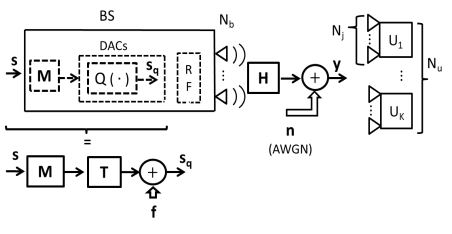
Figure 1: Outline of a quantized massive MU-MIMO downlink system. Upper diagram: some simplified parts of BS. Lower diagram: Bussgang’s theorem applied to the detached part of interest.

We can model the input-output relation of the broadcast channel (BC) as

$$\mathbf{y}=\mathbf{H}\;\mathbf{s}_{q}\>+\>\mathbf{n},$$ (1)

where $\mathbf{y}\in\mathbb{C}^{N_{u}}$ contains the signals received by all users and $\mathbf{H}\in\mathbb{C}^{N_{u}\times N_{b}}$ stands for the matrix which models the assumed broadcast channel that is assumed known to the BS. The entries of $\mathbf{H}$ are considered independent circularly-symmetrical complex Gaussian random variables $\left[\mathbf{H}\right]_{u,b}\in\mathbb{CN}\left(0,1\right)$, $u=1,\cdots,N_{u}$ and $b=1,\cdots,N_{b}$. The noise vector $\mathbf{n}\in\mathbb{C}^{N_{u}}$, is characterized by its i.i.d. circularly-symmetric complex Gaussian entries $n_{u}\in\mathbb{CN}\left(0,\frac{N_{0}}{2}\right)$. We consider that the noise level is known at BS and so is the sampling rate of DACs at BS and ADCs at user equipments. Bussgang’s theorem [7, 8] allows us to express quantized signals as linear functions of the quantized information and distortion expressions, which have no correlation with the signals undergoing quantization. Therefore, the operations performed by the two blocks encompassed by the braces in the upper part of Fig.1 can be transformed in the expression composed of the operations outlined in the lower part. Thus, the quantization $\mathrm{Q}\left(\cdot\right)$ of a precoded symbol vector $\mathbf{Ms}$, where $\mathbf{M}\in\mathbb{C}^{N_{b}\times N_{u}}$ is a precoding matrix and $\mathbf{s}\approx\mathit{N}^{\mathbb{C}}\left(\bm{0}_{N_{u}\times 1},\bm{I}_{N_{u}}\right)$ is the symbol vector, can be expressed by the quantized vector

$$\mathbf{s}_{q}=\mathrm{Q}\left(\mathbf{Ms}\right)=\mathbf{TMs+f},$$ (2)

where the distortion term $\mathbf{f}$ and the symbol $\mathbf{s}$ vectors are uncorrelated. For the general case, $\mathbf{T}\in\mathbb{R}^{N_{b}\times N_{b}}$ is the diagonal matrix expressed by

$$\mathbf{T}_{n,n}= \frac{\alpha\gamma}{\sqrt{\pi}}\mathrm{diag}\left(\mathbf{MM}^{H}\right)^{-1/2}.$$

$$\sum_{l=1}^{J-1}\exp\left(-\gamma^{2}\left(l-\frac{J}{2}\right)^{2}\mathrm{diag}\left(\mathbf{MM}^{H}\right)^{-1}\right)$$ (3)

where $n=1\ldots N_{b}$, and $\mathit{J}$ and $\gamma$ stand for the number of levels and the step size of the quantizer, respectively. The regularization factor $\alpha\in\mathbb{R}$, which will be defined in Subsection II-A, has the purpose of satisfying the average power limitation

$$\mathbb{E}[\parallel\mathbf{Ms}\parallel_{2}^{2}]\leq\mathit{P}$$ (4)

where $\mathit{P}=SNR\>\;\frac{\mathrm{N}_{0}}{2}$.

II-A Achievable sum-rates

In order to compute approximations of achievable sum-rates, in which $N_{b}$ and $N_{u}$ are sufficiently large and that the error resulting from the combination of multiuser interference (MUI) and the distortion from limited resolution of DACs is considered a Gaussian process, we can assume that (II) is the following scalar matrix:

$$\mathbf{T}_{n,n}=\delta\>\mathbf{I}_{Nb\times Nb}$$ (5)

where the entries of $\mathbf{T}_{n,n}$ are given by the Bussgang scalar factor:

$$\delta=\alpha\gamma\sqrt{\frac{N_{b}}{\pi P}}\>\sum_{l=1}^{J-1}\exp\left(-\frac{N_{b}\gamma^{2}}{P}\left(1-\frac{J}{2}\right)^{2}\right)$$ (6)

in which the regularization factor $\alpha$ for enforcing the power constraint (4) is obtained by

$$\alpha= \left(2\mathrm{N_{b}}\gamma^{2}\left(\left(\frac{J-1}{2}\right)^{2}\right.\right.$$

$$\left.\left.-2\sum_{l=1}^{J-1}\left(1-\frac{J}{2}\right)\Xi\left(\sqrt{2N_{b}\gamma^{2}}\left(1-\frac{J}{2}\right)\right)\right)\right)^{-1/2}$$ (7)

where $\Xi\left(w\right)=\int_{-\infty}^{w}\frac{1}{\sqrt{2\pi}}\exp^{-v^{2}/2}\>dv$ [8] is the distributed function of a Gaussian random variable.

It can be proven via Bussgang’s theorem that assuming the system model in Section II and the identity in (5), the sum rate provided by CQA-BD and CQA-RBD precoders can be approximated by

$$\mathit{C}= \log_{2}\left\{\det\left[\mathbf{I}_{Nu}+\delta^{2}\frac{\mathit{SNR}}{\mathit{N}_{u}}\mathbf{\left(HM\right)}\mathbf{\left(HM\right)}^{H}\right.\right.$$

$$\left.\left.\left(\left(1-\delta^{2}\right)\frac{\mathit{SNR}}{\mathit{N}_{u}}\mathbf{\left(HM\right)}\mathbf{\left(HM\right)}^{H}+\mathbf{I}_{Nu}\right)^{-1}\right]\right\}$$ (8)

where the $\mathit{SNR}$ was defined in (4) and $\mathbf{M}$ is the precoding matrix (11), which is defined in Subsection II-B.

It must be highlighted that all process of quantization is concentrated in Bussgang’s factor $\delta$ in (5) and (6). This is one of the contributions of this work, i.e., the derivation of a closed form expression for estimating achievable sum rates based on a scalar factor which characterizes a Bussgang’s gain scalar matrix (5) that approximates the effects of multi-bit quantization. This derivation is provided in the Appendix. The second contribution of this study, which have not been considered in the literature so far, is the application of the obtained closed form expression to evaluate the performance of the achievable sum rates of our proposed CQA-BD and CQA-RBD precoding algorithms under 2,3 and 4-bit quantization.

II-B Review of BD precoding algorithms

It is known [18, 16, 14] that BD is a low-rank technique [24, 25, 26, 27, 28, 29, 30, 86, 32, 33, 34, 35, 46, 36, 37, 38, 39, 40, 41, 42, 43, 48, 45, 47, 48, 49, 50, 51, 52, 53, 54, 55, 71, 72, 58, 59, 60, 61, 62, 63, 64, 65, 66, 67, 68, 69, 89, 71, 72, 73] that employs SVD to design the precoder, which can be performed in two stages. The precoder computed in the first stage suppresses (BD) or attemps to obtain a trade-off between MUI and noise (RBD). Afterwards parallel or near-parallel single user (SU)-MIMO are calculated. The precoder computed in the second stage parallelizes the streams intended for the users. In this way, a precoding matrix $\mathbf{M}_{j}$ related to the jth user can be expressed as a product

$$\mathbf{M}_{j}=\mathbf{M}_{j}^{c}\mathbf{M}_{j}^{d}$$ (9)

in which $\mathbf{M}_{j}^{c}\in\mathbb{C}^{N_{b}\times L_{j}}$ and $\mathbf{M}_{j}^{d}\in\mathbb{C}^{L_{j}\times N_{j}}$. The constant $L_{j}$ depends on which precoding algorithm is chosen (BD or RBD). We can express the combined channel matrix $\mathbf{H}$ and the resulting precoding matrix $\mathbf{M}$ as follows:

$$\mathbf{H}=\left[\mathbf{H}_{1}^{T}\mathbf{H}_{2}^{T}\cdots\mathbf{H}_{K}^{T}\right]^{T}\>\in\mathbb{C}^{N_{u}\times N_{b}}$$ (10)

$$\mathbf{M}=\left[\mathbf{M}_{1}^{T}\mathbf{M}_{2}^{T}\cdots\mathbf{M}_{K}^{T}\right]^{T}\>\in\mathbb{C}^{N_{b}\times N_{u}}$$ (11)

where $\mathbf{H}_{j}\in\mathbb{C}^{N_{j}\times N_{b}}$ is the channel matrix of the $j$th user. The expression $\mathbf{M}_{j}\in\mathbb{C}^{N_{b}\times N_{j}}$ represents the precoding matrix of the $j$th user. For BD precoding algorithm [16], the first factor in (9) is given by

$$\mathbf{M}_{j}^{c\left(BD\right)}=\overline{\mathbf{W}}_{j}^{\left(0\right)}$$ (12)

where $\overline{\mathbf{W}}_{j}^{\left(0\right)}$ is obtained by the SVD [18] of (10), in which the matrix channel of $j$th user was removed, i.e.:

$$\overline{\mathbf{H}}_{j} =\left[\mathbf{H}_{1}^{T}\cdots\mathbf{H}_{j-1}^{T}\mathbf{H}_{j+1}^{T}\cdots\mathbf{H}_{K}^{T}\right]^{T}\>\in\mathbb{C}^{\overline{N}_{j}\times N_{b}}$$

$$=\overline{\mathbf{U}}_{j}\overline{\mathbf{\Phi}}_{j}\overline{\mathbf{W}}_{j}^{H}=\overline{\mathbf{U}}_{j}\overline{\mathbf{\Phi}}_{j}\left[\overline{\mathbf{W}}_{j}^{\left(1\right)}\overline{\mathbf{W}}_{j}^{\left(0\right)}\right]^{H}$$ (13)

where $\overline{N}_{j}=N_{u}-N_{j}$. The matrix $\overline{\mathbf{W}}_{j}^{\left(0\right)}\in\mathbb{C}^{\overline{N}_{b}\times\left(N_{b}-\overline{L}_{j}\right)}$, where $\overline{L}_{j}$ is the assumed rank of $\overline{\mathbf{H}}_{j}$, embraces the ultimate $N_{b}-\overline{L}_{j}$ zero singular vectors. In the case of RBD precoding algorithm, the first factor in (9) is given [16] by

$$\mathbf{M}_{j}^{c\left(RBD\right)}=\overline{\mathbf{W}}_{j}\left(\overline{\mathbf{\Phi}}_{j}^{T}\overline{\mathbf{\Phi}_{j}}+\alpha\mathbf{I}_{N_{b}}\right)^{-1/2}$$ (14)

where $\alpha=\frac{N_{u}\sigma_{n}^{2}}{\mu}$ is the regularization factor and $\mu$ is the whole average transmit power.

The second factor in (9) is obtained by SVD of the effective channel matrix for the $j$th user $\mathbf{H}_{e_{j}}$ and power loading, respectively as follows:

$$\mathbf{M}_{j}^{d\left(BD\right))}=\mathbf{W}_{j}^{\left(1\right)}\>\Gamma^{\left(BD\right)}$$ (15)

$$\mathbf{M}_{j}^{d\left(RBD\right))}=\mathbf{W}_{j}\>\Gamma^{\left(RBD\right)}$$ (16)

where the matrix $\mathbf{W}_{j}^{\left(1\right)}$ embraces the early $\Lambda_{e}=rank\left(\mathbf{H}_{e_{j}}\right)$ singular vectors obtained by the decomposition of $\mathbf{H}_{e_{j}}$, as follows

$$\mathbf{H}_{e_{j}} =\mathbf{H}_{j}\mathbf{M}_{j}^{c}=\mathbf{U}_{j}\mathbf{\Phi}_{j}\mathbf{W}_{j}^{H}$$

$$=\mathbf{U}_{j}\begin{bmatrix}\mathbf{\Phi}_{j}&0\\ 0&0\end{bmatrix}\begin{bmatrix}\mathbf{W}_{j}^{\left(1\right)}&\mathbf{W}_{j}^{\left(0\right)}\end{bmatrix}^{H}$$ (17)

The power loading matrix $\Gamma$ can be obtained by a procedure like water filling (WF)[20].

II-C Increasing requirement of more efficient DACs

Until recently, the use of a modest number of antennas at the BS and their required DACs were not an issue in terms of energy consumption. This is due the fact that DACs consume less energy than ADCs. Despite the diversity of research about DACs, very few allow the calculation of the increment of chip power dissipation as bit resolution increases bit-by-bit, for a fixed technology. In order to roughly compare the consumption of both equipments, we make use of Table I, which contains the fabrication parameters for GaAs 4-bit Analog-to-Digital Converter (AD) and 5-bit Digital-to-Analog (DA) converters, using a 0.7-$\mu$m MESFET self-aligned gate process [21] and the expression proposed in [22].

TABLE I: ADC and DAC fabrication parameters with the same technology

	Resolution	Sampling Rate	Power dissipation
	(bits)	(GHz)	(mW)
ADC	4	1	140
DAC	5	1	85

We start with the expression[22] which relates the power consumed by an ADC to the resolution bits, as follows:

$$\mathrm{P_{ADC}(b)}=\mathrm{c\>\tau\>2^{b}}$$ (18)

where $b$ stands for the resolution bits, $c$ is a constant and $\tau$ is the sampling rate. From (18), we obtain $\frac{\mathrm{P_{ADC}}(4)}{\mathrm{P_{ADC}}(5)}=\frac{1}{2}$, which allows us to estimate $\frac{\mathrm{P_{DAC}}(5)}{\mathrm{P_{ADC}}(5)}=\frac{\mathrm{P_{DAC}}(5)}{2\mathrm{P_{ADC}}(4)}$. With the help of Table (I), we obtain $\mathrm{P_{DAC}}(5)\approx 30\%\mathrm{P_{ADC}}(5)$. So, the DAC consumes around 30 $\%$ of the energy of the ADC with fixed parameter. From the results obtained before, we can roughly estimate the economy in energy by assuming that similarly to ADC, DAC consumption doubles with every extra bit of resolution, i.e., of $\mathcal{O}\left(2^{b}\right)$. Therefore, a decrease in two resolution bits, for instance from 4 to 2 bits, represents a consumption 75$\%$ lower. This reduction of DAC consumption motivates our study.

III Proposed CQA-BD and CQA-RBD precoder algorithm

In this section, we summarize the proposed precoding techniques in Algorithm 1, which encompasses both CQA-BD and its refined variation CQA-RBD. The algorithm starts with the use of the knowledge of the combined channel matrix (10). Then, for a fixed SNR and also a fixed realization of the channel, we perform the calculations from $1$ to $12$ step-by-step, to obtain the precoding matrix $\mathbf{M}$ (11). All operations involved in these steps are detailed in Subsection II-B, which reviews the BD-type precoding algorithms. Next, we calculate the conformation parameter $\alpha$ (II-A), which ensures the power constraint (4), and after this, the Bussgang’s scalar factor (6), which concentrates all process of quantization in the scalar matrix (5). Finally, we can obtain the achievable sum-rates for a fixed SNR and a fixed realization of the channel.

Algorithm 1 Algorithm for estimating CQA-BD and CQA-RBD reachable sums

1:$\mathbf{H}=\left[\mathbf{H}_{1}^{T}\mathbf{H}_{2}^{T}\cdots\mathbf{H}_{K}^{T}\right]^{T}\>\in\mathbb{C}^{N_{u}\times N_{b}}$ (10)

2:for $\mathrm{j=1\;}\colon\>K$ do

3:    $\overline{\mathbf{H}}_{j}=\left[\mathbf{H}_{1}^{T}\cdots\mathbf{H}_{j-1}^{T}\mathbf{H}_{j+1}^{T}\cdots\mathbf{H}_{K}^{T}\right]^{T}\>\in\mathbb{C}^{\overline{N}_{j}\times N_{b}}$(II-B)

4:    $\overline{\mathbf{H}}_{j}=\overline{\mathbf{U}}_{j}\overline{\mathbf{\Phi}}_{j}\overline{\mathbf{W}}_{j}^{H}=\overline{\mathbf{U}}_{j}\overline{\mathbf{\Phi}}_{j}\left[\overline{\mathbf{W}}_{j}^{\left(1\right)}\overline{\mathbf{W}}_{j}^{\left(0\right)}\right]^{H}$ (II-B)

5:    $\mathbf{M}_{j}^{c\left(BD\right)}=\overline{\mathbf{W}}_{j}^{\left(0\right)}$(12)

6:    $\mathbf{M}_{j}^{c\left(RBD\right)}=\overline{\mathbf{W}}_{j}\left(\overline{\mathbf{\Phi}}_{j}^{T}\overline{\mathbf{\Phi}}_{j}+\alpha\mathbf{I}_{N_{b}}\right)^{-1/2}$(14)

7:    $\mathbf{H}_{e_{j}}=\mathbf{H}_{j}\mathbf{M}_{j}^{c}=\mathbf{U}_{j}\mathbf{\Phi}_{j}\mathbf{W}_{j}^{H}=\mathbf{U}_{j}\begin{bmatrix}\mathbf{\Phi}_{j}&0\\ 0&0\end{bmatrix}\begin{bmatrix}\mathbf{W}_{j}^{\left(1\right)}&\mathbf{W}_{j}^{\left(0\right)}\end{bmatrix}^{H}$(II-B)

8:    $\mathbf{\Gamma}^{\left(BD,RBD\right)}\text{by WF \cite[cite]{[\@@bibref{}{Paulraj}{}{}]} or similar}$

9:    $\mathbf{M}_{j}^{d\left(BD\right))}=\mathbf{W}_{j}^{\left(1\right)}\>\Gamma^{\left(BD\right)}$ (15)

10:    $\mathbf{M}_{j}^{d\left(RBD\right))}=\mathbf{W}_{j}\>\Gamma^{\left(RBD\right)}$ (16)

11:    $\mathbf{M}_{j}=\mathbf{M}_{j}^{c}\mathbf{M}_{j}^{d}$(9)

12:end for

13:$\mathbf{M}=\left[\mathbf{M}_{1}^{T}\mathbf{M}_{2}^{T}\cdots\mathbf{M}_{K}^{T}\right]^{T}\>\in\mathbb{C}^{N_{b}\times N_{u}}$ (11)

14:$\begin{aligned} \alpha=&\left(2\mathrm{N_{b}}\gamma^{2}\left(\left(\frac{J-1}{2}\right)^{2}\right.\right.\\ &\left.\left.-2\sum_{l=1}^{J-1}\left(1-\frac{J}{2}\right)\Xi\left(\sqrt{2N_{b}\gamma^{2}}\left(1-\frac{J}{2}\right)\right)\right)\right)^{-1/2}\end{aligned}$ (II-A)

15:$\begin{aligned} \delta=\alpha\gamma\sqrt{\frac{N_{b}}{\pi P}}\sum_{l=1}^{J-1}\exp\left(-\frac{N_{b}\gamma^{2}}{P}\left(1-\frac{J}{2}\right)^{2}\right)\text{Bussgang's scalar factor}\end{aligned}$ (6)

16:$\begin{aligned} \mathit{C}=&\log_{2}\left\{\det\left[\mathbf{I}_{Nu}+\delta^{2}\frac{\mathit{SNR}}{\mathit{N}_{u}}\mathbf{\left(HM\right)}\mathbf{\left(HM\right)}^{H}\right.\right.\\ &\left.\left.\left(\left(1-\delta^{2}\right)\frac{\mathit{SNR}}{\mathit{N}_{u}}\mathbf{\left(HM\right)}\mathbf{\left(HM\right)}^{H}+\mathbf{I}_{Nu}\right)^{-1}\right]\right\}\end{aligned}$ (II-A)

IV Numerical results

We focus our simulations on two scenarios, which are composed of $\left(N_{b1},N_{u1}\right)=\left(32,16\right)$ and $\left(N_{b2},N_{u2}\right)=\left(128,16\right)$, respectively. We model the channel matrix $\mathbf{H}_{j}$ of the $j$th user with entries given by complex Gaussian random variables with zero mean and unit variance. In addition, it is assumed that the channel is static while each packet is transmitted and that the antennas are uncorrelated. The channel estimation is considered ideal at the receive side and there is no error in the feedback of the channel information to the receiver. We set the trials to $2\times 10^{2}$ and the packet length to $10^{2}$ symbols.

Fig.2 depicts the sum-rates of the proposed CQA-BD and CQA-RBD algorithms, based on Bussgang’s theorem, under 2 and 3-bit quantization, corresponding to $\mathrm{J}=\left\{8,4\right\}$ levels of quantization, and employing the first scenario $\left(N_{b1},N_{u1}\right)=\left(32,16\right)$. For the purpose of comparisons, we have also included the sum-rate of CQA-ZF, which represents the same technique used in CQA-BD type, applied to Zero-Forcing (ZF). They are compared to the RBD (refined variant of BD), the standard BD, and ZF, at upper side, all of them in full resolution (RBD FR, BD FR, ZF FR). They are also compared to RBD under 2 and 3-bit roughly standard quantization, i.e., not using Bussgang’s theorem. It is possible to notice four well-defined ranked groups of curves in the range $\left[7\>20\right]$ and that, in the same range, the rank of each group is also clear. Thus, the inequalities Sum RBD$>$ Sum BD $>$ Sum ZF is preserved, regardless of quantization. It is also clear the influence of the levels of quantization on the the sum-rates. We highlight the clear gaps between each group of sum-rates achieved corresponding to each level of quantization. It can be noticed the significant increasing gaps from 2-3bit roughly quantized (RBDqr), at the bottom, to 2-3bits and CQA-RBD, and how close 3-bit CQA-RBD is to full resolution (FR) RBD. Based on Subsection II-C, the performance of CQA-RBD and CQA-BD under 2-3 bits quantization, which increasingly approximates RBD FR and BD FR, indicating a corresponding saving in energy.

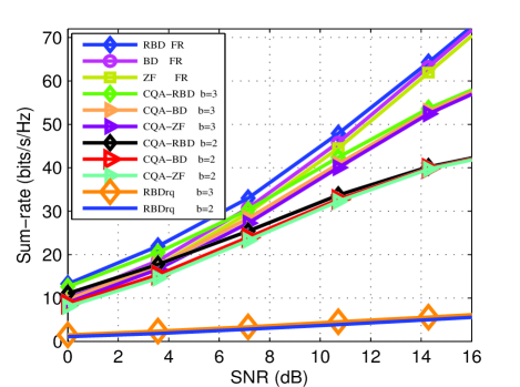
Figure 2: Approximations of reachable rates via Bussgang theorem assuming Gaussian signals for CQA-RBD, CQA-BD and CQA-ZF algorithms, $N_{b}=32$ and $N_{u}=16$. Decreasing levels of quantization from the upper side to the middle $\left(N_{b1},N_{u1}\right)=\left(32,16\right)$. At the bottom, the roughly quantized RBDrq for $\mathrm{J}=\left\{8,4\right\}$

Fig. 3 illustrates the performance of the sum-rates in the second configuration mentioned before, i.e., $\left(N_{b2},N_{u2}\right)=\left(128,16\right)$. In this arrangement, we compare only 2,3,4-bit CQA-BD class to 2,3-bit RBDrq (roughly quantized) and RBD FR,BD FR. It can be noticed that the curves depicting CQA-RBD and CQA-BD at each level of quantization are almost similar, which can be justified by the increase of transmit antennas. However the aim of the figure is to show more clearly how 2,3,4-bit CQA-RBD and CQA-BD algorithms increase sum-rates, comparing them to a bad condition, i.e., 2,3-bit RBDrq and to a ideal condition RBD-FR. Taking RBD FR as a reference at 3.57 and 7.14 dB, the sum-rate achieved by 2-bit CQA-RBD, represents $80\%$ and $74\%$, respectively, of the rates achieved with a full-resolution system. For 3-bit CQA-RBD, at the same range, the sum-rate achieves $93\%$ and $90\%$, respectively, of that achieved by full resolution. This means substantially less energy dissipated at the cost of slightly lower sum-rates, which justify to the investigation of low-resolution precoding techniques using 2,3 bits as an alternative of 1-bit quantization-based precoders. Future work will include the development of detection and decoding techniques [74, 75, 76, 77, 78, 79, 80, 81, 82, 83, 84, 85, 86, 92, 93, 94, 95, 96, 97, 98, 99, 100]

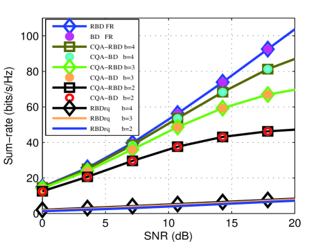
Figure 3: Approximations of reachable rates via Bussgang theorem assuming Gaussian signals for CQA-BD and CQA-RBD algorithms, $N_{b}=128$ and $N_{u}=16$. Decreasing levels of quantization from upper side to the middle $\mathrm{J}=\left\{\infty,16,8,4\right\}$. At the bottom, the roughly quantized RBDrq for $\mathrm{J}=\left\{16,8,4\right\}$

V Conclusions

Founded on Bussgang’s theorem, which allows us to express quantized signal as linear functions of the quantized information and distortion, we have proposed the CQA-BD and CQA-RBD precoding algorithms for multi-bit DACs, in particular, using 2,3,4-bit quantization.These approaches have not been taken into account in the literature so far. We have also justified the need for reducing the energy consumption in DACs by using few bits of quantization, as a way of compensating the increase of power dissipation resulting from modern large-scale MIMO systems. Compared to the current full resolution RBD and BED algorithms and coarsely quantized RBD algorithm, the sum-rates obtained by CQA-RBD and BD achieve significant gains. Here we provide the derivation of (II-A).

-A Assumptions

According to Subsection II, we assume that the cross covariance matrices $\mathbf{R}_{sf}=\mathbb{E}[\mathbf{s}\mathbf{f}^{H}]$ and $\mathbf{R}_{sn}=\mathbb{E}[\mathbf{s}\mathbf{n}^{H}]$ and $\mathbf{R}_{fn}=\mathbb{E}[\mathbf{f}\mathbf{n}^{H}]$ are all of them equal to zero and so are $\mathbf{R}_{fs}$, $\mathbf{R}_{ns}$ and $\mathbf{R}_{nf}$. Additionally, as stated in Subsection 5, the distortion vector is assumed to be Gaussian.

-B Development

We start by combining (1) with (2), obtaining:

$$\mathbf{y}=\mathbf{HTMs}+\mathbf{Hf}\>+\>\mathbf{n},$$ (19)

where we can define a distortion-plus-noise vector

$$\mathbf{\tilde{n}}=\mathbf{Hf}\>+\>\mathbf{n}.$$ (20)

We can estimate the correlation matrix $\mathbf{R}_{sqsq}$ of the quantized vector (2), as follows:

$$\mathbf{R}_{sqsq} =\mathbb{E}[\mathbf{(TMs+f)}\mathbf{(TMs+f)}^{H}]$$

$$=\mathbb{E}[\mathbf{TMs}\mathbf{s}^{H}\mathbf{M}^{H}\mathbf{T}^{H}+\mathbf{f}\mathbf{f}^{H}]$$

$$=\delta^{2}\sigma^{2}\mathbf{M}\mathbf{M}^{H}+\mathbf{R}_{ff},$$ (21)

where we made use of (5) and the autocorrelation matrix of the symbol vector $\mathbf{R}_{ss}=\mathbb{E}[\mathbf{s}\mathbf{s}^{H}]=\sigma_{s}^{2}\mathbf{I}_{Nu}$, in which $\sigma_{s}^{2}$ is its variance. The term $\mathbf{R}_{ff}=\mathbb{E}[\mathbf{f}\mathbf{f}^{H}]$ stands for the autocorrelation of the distortion vector $\mathbf{f}$.

Next, we can notice that in full resolution, since there is no quantization and its associated distortion, (2) turns into

$$\ \mathbf{s}_{q}=\mathbf{Ms},$$ (22)

where we make $\mathbf{T}_{n,n}=\mathbf{I}_{Nb\times Nb}$, i.e., $\delta=1$ in (5), and assume that $\mathbf{f}=\textbf{0}_{Nb}$.

Now, we calculate the autocorrelation of the full resolution precoded symbol vector (22) as follows:

$$\mathbf{R}_{sqsq} =\mathbb{E}[\mathbf{(Ms)}\mathbf{(Ms)}^{H}]$$

$$=\mathbb{E}[\mathbf{Ms}\mathbf{s}^{H}\mathbf{M}^{H}]$$

$$=\sigma_{s}^{2}\mathbf{M}\mathbf{M}^{H},$$ (23)

By equating (-B) and (-B), we can obtain the expression of the autocorrelation of the distortion vector $\mathbf{R}_{ff}$:

$$\delta^{2}\sigma_{s}^{2}\mathbf{M}\mathbf{M}^{H}+\mathbf{R}_{ff}=\sigma_{s}^{2}\mathbf{M}\mathbf{M}^{H}$$

$$\therefore\mathbf{R}_{ff}=\left(1-\delta^{2}\right)\sigma_{s}^{2}\mathbf{M}\mathbf{M}^{H}$$ (24)

By equating (-B) and (-B), we can obtain the expression of the autocorrelation of the distortion vector $\mathbf{R}_{ff}$:

$$\delta^{2}\sigma_{s}^{2}\mathbf{M}\mathbf{M}^{H}+\mathbf{R}_{ff}=\sigma_{s}^{2}\mathbf{M}\mathbf{M}^{H}$$

$$\therefore\mathbf{R}_{ff}=\left(1-\delta^{2}\right)\sigma_{s}^{2}\mathbf{M}\mathbf{M}^{H}$$ (25)

We can then compute the autocorrelation matrix of (19), obtaining:

$$\mathbf{R}_{yy} =\mathbb{E}[\mathbf{y}\mathbf{y}^{H}]$$

$$=\left(\mathbf{HTM}\right)\>\mathbf{R}_{ss}\left(\mathbf{HTM}\right)^{H}$$

$$+\mathbf{H}\>\mathbf{R}_{ff}\mathbf{H}^{H}\>+\>\mathbf{R}_{nn},$$ (26)

where $\mathbf{R}_{ss}=\mathbb{E}[\mathbf{s}\mathbf{s}^{H}]$, $\mathbf{R}_{ff}=\mathbb{E}[\mathbf{f}\mathbf{f}^{H}]$ and $\mathbf{R}_{nn}=\mathbb{E}[\mathbf{n}\mathbf{n}^{H}]$ are the autocorrelation matrices of the signal, the distortion and the noise vectors, respectively. Similar procedure applied to the distortion-plus-noise vector (20), considering the conditions above, yields:

$$\mathbf{R}_{\tilde{n}\tilde{n}}=\mathbb{E}[{\tilde{\mathbf{n}}\tilde{\mathbf{n}}^{H}}]=\mathbf{H}\mathbf{R}_{ff}\mathbf{H}_{H}+\mathbf{R}_{nn},$$ (27)

From the principles of information theory [23] and the capacity of a frequency flat deterministic MIMO channel [20], we can bound the achievable rate in bits per channel use at which information can be sent with arbitrarily low probability of error by the mutual information of a Gaussian channel, i.e.

$$\mathit{C}\leqq\mathit{I}\left(\mathbf{s},\mathbf{y}\right) =\Upsilon\left(\mathbf{y}\right)-\Upsilon\left(\mathbf{y}\rvert\mathbf{s}\right)$$

$$=\Upsilon\left(\mathbf{y}\right)-\Upsilon\left(\mathbf{\tilde{n}}\right)$$

$$=\log_{2}\left[\det\left(\pi e\mathbf{R}_{yy}\right)\right]-\log_{2}\left[\det\left(\pi e\mathbf{R}_{\tilde{n}\tilde{n}}\right)\right]$$

$$=\log_{2}\left[\det\left(\mathbf{R}_{yy}\right)\right]-\log_{2}\left[\det\left(\mathbf{R}_{\tilde{n}\tilde{n}}\right)\right]$$

$$=\log_{2}\left[\det\left(\mathbf{R}_{yy}\mathbf{R}^{-1}_{\tilde{n}\tilde{n}}\right)\right]$$ (28)

where $\Upsilon\left(\mathbf{y}\right)$ and $\Upsilon\left(\mathbf{y}\rvert\mathbf{s}_{q}\right)$ are the differential and the conditional differential entropies of $\mathbf{y}$, respectively.

By combining (-B) and (27) with (-B), we have:

$$\mathit{C} \leqq\log_{2}\left\{\det\left[\left(\left(\mathbf{HTM}\right)\>\mathbf{R}_{ss}\left(\mathbf{HTM}\right)^{H}\right)\right.\right.$$

$$\left.\left.\left(\mathbf{H}\mathbf{R}_{ff}\mathbf{H}^{H}+\mathbf{R}_{nn}\right)^{-1}+\mathbf{I}_{N_{u}}\right]\right\}$$ (29)

In Section II, (4), we have defined the total power as $\mathit{P}=\mathit{SNR}\>\frac{\mathrm{N}_{0}}{2}$. From the definition of the noise vector, also in that Section, we can express its covariance matrix as $\mathbf{R}_{nn}=\frac{\mathrm{N}_{0}}{2}\mathbf{I}_{N_{u}}$ Combining the two previously mentioned expressions, we obtain

$$\mathbf{R}_{nn}=\frac{\mathit{P}}{SNR}\;\mathbf{I}_{N_{u}}$$ (30)

Recalling, from Section II, that $\mathbf{R}_{ss}\approx\mathbf{I}_{N_{u}}$, and assuming that the total power is given by $\mathit{P}=trace\left(\mathbf{R}_{ss}\right)=N_{u}$, (30) turns into:

$$\mathbf{R}_{nn}=\frac{\mathit{N_{u}}}{SNR}\;\mathbf{I}_{N_{u}}$$ (31)

By combining (-B), (-B) (5) and the expression of $\mathbf{R}_{ss}$ previously mentioned with (31), followed by algebraic manipulation, we can obtain:

$$\mathit{C}= \log_{2}\left\{\det\left[\mathbf{I}_{Nu}+\delta^{2}\frac{\mathit{SNR}}{\mathit{N}_{u}}\mathbf{\left(HM\right)}\mathbf{\left(HM\right)}^{H}\right.\right.$$

$$\left.\left.\left(\left(1-\delta^{2}\right)\frac{\mathit{SNR}}{\mathit{N}_{u}}\mathbf{\left(HM\right)}\mathbf{\left(HM\right)}^{H}+\mathbf{I}_{Nu}\right)^{-1}\right]\right\}\qed$$ (32)

References

- [1] Rusek, F. et al: ’Scaling up MIMO: Opportunities and challenges with very large large arrays’, IEEE Signal Process. Mag., 30, (1), pp.40-60, Jan. 2013.
- [2] Larsson, E. G., Edfors, O., Tufvesson, F., Marzetta, T. L.: ’Massive MIMO for next generation wireless systems’, IEEE Commun. Mag, 52, (2), pp.186-195, Feb. 2014.
- [3] Lu, L., Li,G.Y., Swindlehurst, A. L., Ashikhmin, A., Zhang, R.: ’An overview of massive MIMO: Benefits and challenges’, IEEE J. Sel. Topics Signal Process., 8, (5), pp.742-758, Oct. 2014.
- [4] Sarajlic, M., Liu, L., Swindlehurst, A. L., Edfors, O., ’An overview of massive MIMO: Benefits and challenges’, Proc. 50th Asilomar Conference on Signals, Systems and Computers, pp. 1-6, 2016.
- [5] de Lamare, R. C., ”Massive MIMO systems: Signal processing challenges and future trends,” in URSI Radio Science Bulletin, vol. 2013, no. 347, pp. 8-20, Dec. 2013.
- [6] Zhang, W., et al., ”Large-Scale Antenna Systems With UL/DL Hardware Mismatch: Achievable Rates Analysis and Calibration,” IEEE Transactions on Communications, vol. 63, no. 4, pp. 1216-1229, April 2015.
- [7] Bussgang, J. J., ’Crosscorrelation functions of amplitude-distorted Gaussian signals’, Res. Lab. Electron., Cambridge, MA, USA, Tech. Rep. 216, Mar. 1952.
- [8] Jacobsson, S., Durisi, G., Coldrey, M., Goldstein,T., Studer, C., ’Quantized precoding for massive MU-MIMO’, IEEE Trans. on Communications, 65, (11), Nov. 2017.
- [9] Jacobsson, S., Durisi, G., Coldrey, M., Studer, C., ’Linear Precoding With Low-Resolution DACs for Massive MU-MIMO-OFDM Downlink’, IEEE Transactions on Wireless Communications, 18 , (3) , Mar. 2019.
- [10] Jacobsson, S., Durisi, G., Coldrey, M., Gustavsson, U., Studer, C., ’Throughput Analysis of Massive MIMO Uplink With Low-Resolution ADCs’, IEEE Transactions on Wireless Communications, 16 , (6) , Jun. 2017.
- [11] Rowe, H., ’Memoryless nonlinearities with Gaussian inputs: Elementary results’, Bell System Technical Journal, 61, (7), pp.1519-1525, Sep. 1982.
- [12] Landau, L, T. N., Lamare, R. C., ’Branch-and-Bound Precoding for Multiuser MIMO Systems With 1-Bit Quantization’, IEEE Wireless Communications Letters, 6,(6), Dec. 2017
- [13] Mezghani, A., Ghiat, R., Nossek, J. A,. ’Transmit processing with low resolution D/A-converters’, 16th IEEE International Conference on Electronics, Circuits and Systems, pp.1-4, 2009.
- [14] Spencer, Q. H. , Swindlehurst, A. L. and Haardt, M., ”Zero-forcing methods for downlink spatial multiplexing in multiuser MIMO channels,” in IEEE Transactions on Signal Processing, vol. 52, no. 2, pp. 461-471, Feb. 2004.
- [15] Sung, H., Lee, S., Lee, I., ’Generalized Channel Inversion Methods for Multiuser MIMO Systems’, IEEE Transactions on Communications, 57, (11), Nov. 2009.
- [16] Stankovic, V., Haardt, M., ’Generalized Design of Multi-User MIMO Precoding Matrices’, IEEE Transactions on Wireles Communications, 7, (3), Mar. 2008.
- [17] Zu, K. and de Lamare R. C., ”Low-Complexity Lattice Reduction-Aided Regularized Block Diagonalization for MU-MIMO Systems,” in IEEE Communications Letters, vol. 16, no. 6, pp. 925-928, June 2012.
- [18] Zu, K., Lamare, R. C., and Haardt, M., ’Generalized Design of Low-Complexity Block Diagonalization Type Precoding Algorithms for Multiuser MIMO Systems’, IEEE Transactions on Communications, 61, (10), Oct. 2013.
- [19] Zhang, W. et al., ”Widely Linear Precoding for Large-Scale MIMO with IQI: Algorithms and Performance Analysis,” IEEE Transactions on Wireless Communications, vol. 16, no. 5, pp. 3298-3312, May 2017.
- [20] Paulraj, A., Nabar, R., Gore, D., ’Introduction to Space-Time Wireless Communications’, Cambridge University Press, 2003.
- [21] Naber, J., Singh, H. , Sadler, R., Milan, J., ’A low-power, high-speed 4-bit GAAS ADC and 5-bit DAC’, Proc. 11th Annu. Gallium Arsenide Integr. Circuit Symp., San Diego, CA, USA, pp.333-336, Oct. 1989.
- [22] Orhan, O., Erkip, E., Rangan, S., ’Low power analog-to-digital converter in millimiter wave systems: Impact of resolution and bandwidth on performance’, Information theory and Applications Workshop, pp. 191-198, Feb.2015.
- [23] Cover, T.H., Thomas, J. A., ’Elements of Information Theory’, Second Edition, Wiley, 2006.
- [24] Z. Xu and M.K. Tsatsanis, “Blind adaptive algorithms for minimum variance CDMA receivers,” IEEE Trans. Communications, vol. 49, No. 1, January 2001.
- [25] R. C. de Lamare and R. Sampaio-Neto, “Low-Complexity Variable Step-Size Mechanisms for Stochastic Gradient Algorithms in Minimum Variance CDMA Receivers”, IEEE Trans. Signal Processing, vol. 54, pp. 2302 - 2317, June 2006.
- [26] C. Xu, G. Feng and K. S. Kwak, “A Modified Constrained Constant Modulus Approach to Blind Adaptive Multiuser Detection,” IEEE Trans. Communications, vol. 49, No. 9, 2001.
- [27] Z. Xu and P. Liu, “Code-Constrained Blind Detection of CDMA Signals in Multipath Channels,” IEEE Sig. Proc. Letters, vol. 9, No. 12, December 2002.
- [28] R. C. de Lamare and R. Sampaio Neto, ”Blind Adaptive Code-Constrained Constant Modulus Algorithms for CDMA Interference Suppression in Multipath Channels”, IEEE Communications Letters, vol 9. no. 4, April, 2005.
- [29] L. Landau, R. C. de Lamare and M. Haardt, “Robust adaptive beamforming algorithms using the constrained constant modulus criterion,” IET Signal Processing, vol.8, no.5, pp.447-457, July 2014.
- [30] R. C. de Lamare, “Adaptive Reduced-Rank LCMV Beamforming Algorithms Based on Joint Iterative Optimisation of Filters”, Electronics Letters, vol. 44, no. 9, 2008.
- [31] R. C. de Lamare and R. Sampaio-Neto, “Adaptive Reduced-Rank Processing Based on Joint and Iterative Interpolation, Decimation and Filtering”, IEEE Transactions on Signal Processing, vol. 57, no. 7, July 2009, pp. 2503 - 2514.
- [32] R. C. de Lamare and Raimundo Sampaio-Neto, “Reduced-rank Interference Suppression for DS-CDMA based on Interpolated FIR Filters”, IEEE Communications Letters, vol. 9, no. 3, March 2005.
- [33] R. C. de Lamare and R. Sampaio-Neto, “Adaptive Reduced-Rank MMSE Filtering with Interpolated FIR Filters and Adaptive Interpolators”, IEEE Signal Processing Letters, vol. 12, no. 3, March, 2005.
- [34] R. C. de Lamare and R. Sampaio-Neto, “Adaptive Interference Suppression for DS-CDMA Systems based on Interpolated FIR Filters with Adaptive Interpolators in Multipath Channels”, IEEE Trans. Vehicular Technology, Vol. 56, no. 6, September 2007.
- [35] R. C. de Lamare, “Adaptive Reduced-Rank LCMV Beamforming Algorithms Based on Joint Iterative Optimisation of Filters,” Electronics Letters, 2008.
- [36] R. C. de Lamare and R. Sampaio-Neto, “Reduced-rank adaptive filtering based on joint iterative optimization of adaptive filters”, IEEE Signal Process. Lett., vol. 14, no. 12, pp. 980-983, Dec. 2007.
- [37] R. C. de Lamare, M. Haardt, and R. Sampaio-Neto, “Blind Adaptive Constrained Reduced-Rank Parameter Estimation based on Constant Modulus Design for CDMA Interference Suppression”, IEEE Transactions on Signal Processing, June 2008.
- [38] M. Yukawa, R. C. de Lamare and R. Sampaio-Neto, “Efficient Acoustic Echo Cancellation With Reduced-Rank Adaptive Filtering Based on Selective Decimation and Adaptive Interpolation,” IEEE Transactions on Audio, Speech, and Language Processing, vol.16, no. 4, pp. 696-710, May 2008.
- [39] R. C. de Lamare and R. Sampaio-Neto, “Reduced-rank space-time adaptive interference suppression with joint iterative least squares algorithms for spread-spectrum systems,” IEEE Trans. Vehi. Technol., vol. 59, no. 3, pp. 1217-1228, Mar. 2010.
- [40] R. C. de Lamare and R. Sampaio-Neto, “Adaptive reduced-rank equalization algorithms based on alternating optimization design techniques for MIMO systems,” IEEE Trans. Vehi. Technol., vol. 60, no. 6, pp. 2482-2494, Jul. 2011.
- [41] R. C. de Lamare, L. Wang, and R. Fa, “Adaptive reduced-rank LCMV beamforming algorithms based on joint iterative optimization of filters: Design and analysis,” Signal Processing, vol. 90, no. 2, pp. 640-652, Feb. 2010.
- [42] R. Fa, R. C. de Lamare, and L. Wang, “Reduced-Rank STAP Schemes for Airborne Radar Based on Switched Joint Interpolation, Decimation and Filtering Algorithm,” IEEE Transactions on Signal Processing, vol.58, no.8, Aug. 2010, pp.4182-4194.
- [43] L. Wang and R. C. de Lamare, ”Low-Complexity Adaptive Step Size Constrained Constant Modulus SG Algorithms for Blind Adaptive Beamforming”, Signal Processing, vol. 89, no. 12, December 2009, pp. 2503-2513.
- [44] L. Wang and R. C. de Lamare, “Adaptive Constrained Constant Modulus Algorithm Based on Auxiliary Vector Filtering for Beamforming,” IEEE Transactions on Signal Processing, vol. 58, no. 10, pp. 5408-5413, Oct. 2010.
- [45] L. Wang, R. C. de Lamare, M. Yukawa, ”Adaptive Reduced-Rank Constrained Constant Modulus Algorithms Based on Joint Iterative Optimization of Filters for Beamforming,” IEEE Transactions on Signal Processing, vol.58, no.6, June 2010, pp.2983-2997.
- [46] L. Qiu, Y. Cai, R. C. de Lamare and M. Zhao, “Reduced-Rank DOA Estimation Algorithms Based on Alternating Low-Rank Decomposition,” IEEE Signal Processing Letters, vol. 23, no. 5, pp. 565-569, May 2016.
- [47] L. Wang, R. C. de Lamare and M. Yukawa, “Adaptive reduced-rank constrained constant modulus algorithms based on joint iterative optimization of filters for beamforming”, IEEE Transactions on Signal Processing, vol.58, no. 6, pp. 2983-2997, June 2010.
- [48] L. Wang and R. C. de Lamare, “Adaptive constrained constant modulus algorithm based on auxiliary vector filtering for beamforming”, IEEE Transactions on Signal Processing, vol. 58, no. 10, pp. 5408-5413, October 2010.
- [49] R. Fa and R. C. de Lamare, “Reduced-Rank STAP Algorithms using Joint Iterative Optimization of Filters,” IEEE Transactions on Aerospace and Electronic Systems, vol.47, no.3, pp.1668-1684, July 2011.
- [50] Z. Yang, R. C. de Lamare and X. Li, “L1-Regularized STAP Algorithms With a Generalized Sidelobe Canceler Architecture for Airborne Radar,” IEEE Transactions on Signal Processing, vol.60, no.2, pp.674-686, Feb. 2012.
- [51] Z. Yang, R. C. de Lamare and X. Li, “Sparsity-aware space–time adaptive processing algorithms with L1-norm regularisation for airborne radar”, IET signal processing, vol. 6, no. 5, pp. 413-423, 2012.
- [52] Neto, F.G.A.; Nascimento, V.H.; Zakharov, Y.V.; de Lamare, R.C., ”Adaptive re-weighting homotopy for sparse beamforming,” in Signal Processing Conference (EUSIPCO), 2014 Proceedings of the 22nd European , vol., no., pp.1287-1291, 1-5 Sept. 2014
- [53] Almeida Neto, F.G.; de Lamare, R.C.; Nascimento, V.H.; Zakharov, Y.V.,“Adaptive reweighting homotopy algorithms applied to beamforming,” IEEE Transactions on Aerospace and Electronic Systems, vol.51, no.3, pp.1902-1915, July 2015.
- [54] L. Wang, R. C. de Lamare and M. Haardt, “Direction finding algorithms based on joint iterative subspace optimization,” IEEE Transactions on Aerospace and Electronic Systems, vol.50, no.4, pp.2541-2553, October 2014.
- [55] S. D. Somasundaram, N. H. Parsons, P. Li and R. C. de Lamare, “Reduced-dimension robust capon beamforming using Krylov-subspace techniques,” IEEE Transactions on Aerospace and Electronic Systems, vol.51, no.1, pp.270-289, January 2015.
- [56] H. Ruan and R. C. de Lamare, “Robust adaptive beamforming using a low-complexity shrinkage-based mismatch estimation algorithm,” IEEE Signal Process. Lett., vol. 21 no. 1 pp. 60-64, Nov. 2013.
- [57] H. Ruan and R. C. de Lamare, “Robust Adaptive Beamforming Based on Low-Rank and Cross-Correlation Techniques,” IEEE Transactions on Signal Processing, vol. 64, no. 15, pp. 3919-3932, Aug. 2016.
- [58] S. Xu and R.C de Lamare, , Distributed conjugate gradient strategies for distributed estimation over sensor networks, Sensor Signal Processing for Defense SSPD, September 2012.
- [59] S. Xu, R. C. de Lamare, H. V. Poor, “Distributed Estimation Over Sensor Networks Based on Distributed Conjugate Gradient Strategies”, IET Signal Processing, 2016 (to appear).
- [60] S. Xu, R. C. de Lamare and H. V. Poor, Distributed Compressed Estimation Based on Compressive Sensing, IEEE Signal Processing letters, vol. 22, no. 9, September 2014.
- [61] S. Xu, R. C. de Lamare and H. V. Poor, “Distributed reduced-rank estimation based on joint iterative optimization in sensor networks,” in Proceedings of the 22nd European Signal Processing Conference (EUSIPCO), pp.2360-2364, 1-5, Sept. 2014
- [62] S. Xu, R. C. de Lamare and H. V. Poor, “Adaptive link selection strategies for distributed estimation in diffusion wireless networks,” in Proc. IEEE International Conference onAcoustics, Speech and Signal Processing (ICASSP), , vol., no., pp.5402-5405, 26-31 May 2013.
- [63] S. Xu, R. C. de Lamare and H. V. Poor, “Dynamic topology adaptation for distributed estimation in smart grids,” in Computational Advances in Multi-Sensor Adaptive Processing (CAMSAP), 2013 IEEE 5th International Workshop on , vol., no., pp.420-423, 15-18 Dec. 2013.
- [64] S. Xu, R. C. de Lamare and H. V. Poor, “Adaptive Link Selection Algorithms for Distributed Estimation”, EURASIP Journal on Advances in Signal Processing, 2015.
- [65] T. G. Miller, S. Xu, R. C. de Lamare and H. V. Poor, “Distributed Spectrum Estimation Based on Alternating Mixed Discrete-Continuous Adaptation,” IEEE Signal Processing Letters, vol. 23, no. 4, pp. 551-555, April 2016.
- [66] N. Song, R. C. de Lamare, M. Haardt, and M. Wolf, “Adaptive Widely Linear Reduced-Rank Interference Suppression based on the Multi-Stage Wiener Filter,” IEEE Transactions on Signal Processing, vol. 60, no. 8, 2012.
- [67] N. Song, W. U. Alokozai, R. C. de Lamare and M. Haardt, “Adaptive Widely Linear Reduced-Rank Beamforming Based on Joint Iterative Optimization,” IEEE Signal Processing Letters, vol.21, no.3, pp. 265-269, March 2014.
- [68] R.C. de Lamare, R. Sampaio-Neto and M. Haardt, ”Blind Adaptive Constrained Constant-Modulus Reduced-Rank Interference Suppression Algorithms Based on Interpolation and Switched Decimation,” IEEE Trans. on Signal Processing, vol.59, no.2, pp.681-695, Feb. 2011.
- [69] Y. Cai, R. C. de Lamare, “Adaptive Linear Minimum BER Reduced-Rank Interference Suppression Algorithms Based on Joint and Iterative Optimization of Filters,” IEEE Communications Letters, vol.17, no.4, pp.633-636, April 2013.
- [70] R. C. de Lamare and R. Sampaio-Neto, “Sparsity-Aware Adaptive Algorithms Based on Alternating Optimization and Shrinkage,” IEEE Signal Processing Letters, vol.21, no.2, pp.225,229, Feb. 2014.
- [71] H. Ruan and R. C. de Lamare, “Robust adaptive beamforming using a low-complexity shrinkage-based mismatch estimation algorithm,” IEEE Signal Process. Lett., vol. 21 no. 1 pp. 60-64, Nov. 2013.
- [72] H. Ruan and R. C. de Lamare, “Robust Adaptive Beamforming Based on Low-Rank and Cross-Correlation Techniques,” IEEE Transactions on Signal Processing, vol. 64, no. 15, pp. 3919-3932, Aug. 2016.
- [73] H. Ruan and R. C. de Lamare, ”Distributed Robust Beamforming Based on Low-Rank and Cross-Correlation Techniques: Design and Analysis,” in IEEE Transactions on Signal Processing, vol. 67, no. 24, pp. 6411-6423, 15 Dec.15, 2019.
- [74] R. C. de Lamare, ”Massive MIMO systems: Signal processing challenges and future trends,” URSI Radio Science Bulletin, vol. 2013, no. 347, pp. 8-20, Dec. 2013.
- [75] W. Zhang et al., ”Large-Scale Antenna Systems With UL/DL Hardware Mismatch: Achievable Rates Analysis and Calibration,” IEEE Transactions on Communications, vol. 63, no. 4, pp. 1216-1229, April 2015.
- [76] P. Li, R. C. de Lamare and R. Fa, “Multiple Feedback Successive Interference Cancellation Detection for Multiuser MIMO Systems”, IEEE Trans. on Wireless Comm., vol. 10, no. 8, pp. 2434-2439, Aug. 2011.
- [77] R. C. de Lamare and R. Sampaio-Neto, ”Adaptive MBER decision feedback multiuser receivers in frequency selective fading channels,” IEEE Communications Letters, vol. 7, no. 2, pp. 73-75, Feb. 2003.
- [78] R. C. De Lamare, R. Sampaio-Neto and A. Hjorungnes, ”Joint iterative interference cancellation and parameter estimation for cdma systems,” IEEE Communications Letters, vol. 11, no. 12, pp. 916-918, December 2007.
- [79] R. C. De Lamare and R. Sampaio-Neto, “Minimum Mean-Squared Error Iterative Successive Parallel Arbitrated Decision Feedback Detectors for DS-CDMA Systems,” IEEE Transactions on Communications, vol. 56, no. 5, pp. 778-789, May 2008.
- [80] Y. Cai and R. C. de Lamare, ”Space-Time Adaptive MMSE Multiuser Decision Feedback Detectors With Multiple-Feedback Interference Cancellation for CDMA Systems,” IEEE Transactions on Vehicular Technology, vol. 58, no. 8, pp. 4129-4140, Oct. 2009.
- [81] R. C. de Lamare and R. Sampaio-Neto, ”Adaptive Reduced-Rank Equalization Algorithms Based on Alternating Optimization Design Techniques for MIMO Systems,” IEEE Transactions on Vehicular Technology, vol. 60, no. 6, pp. 2482-2494, July 2011.
- [82] P. Li and R. C. De Lamare, ”Adaptive Decision-Feedback Detection With Constellation Constraints for MIMO Systems,” IEEE Transactions on Vehicular Technology, vol. 61, no. 2, pp. 853-859, Feb. 2012.
- [83] R. C. de Lamare, “Adaptive and Iterative Multi-Branch MMSE Decision Feedback Detection Algorithms for Multi-Antenna Systems,” IEEE Transactions on Wireless Communications, vol. 12, no. 10, pp. 5294-5308, October 2013.
- [84] P. Li and R. C. de Lamare, ”Distributed Iterative Detection With Reduced Message Passing for Networked MIMO Cellular Systems,” IEEE Transactions on Vehicular Technology, vol. 63, no. 6, pp. 2947-2954, July 2014.
- [85] Y. Cai, R. C. de Lamare, B. Champagne, B. Qin and M. Zhao, ”Adaptive Reduced-Rank Receive Processing Based on Minimum Symbol-Error-Rate Criterion for Large-Scale Multiple-Antenna Systems,” IEEE Transactions on Communications, vol. 63, no. 11, pp. 4185-4201, Nov. 2015.
- [86] R. C. de Lamare and R. Sampaio-Neto, ”Adaptive Reduced-Rank Processing Based on Joint and Iterative Interpolation, Decimation, and Filtering,” in IEEE Transactions on Signal Processing, vol. 57, no. 7, pp. 2503-2514, July 2009.
- [87] D. Angelosante, J. A. Bazerque and G. B. Giannakis, “Online adaptive estimation of sparse signals: where RLS meets the -norm,” IEEE Trans. Sig. Proc., vol. 58, no. 7, pp. 3436-3446, 2010.
- [88] Z. Yang, R. C. de Lamare and X. Li, ” -Regularized STAP Algorithms With a Generalized Sidelobe Canceler Architecture for Airborne Radar,” in IEEE Transactions on Signal Processing, vol. 60, no. 2, pp. 674-686, Feb. 2012.
- [89] R. C. de Lamare and R. Sampaio-Neto, ”Sparsity-Aware Adaptive Algorithms Based on Alternating Optimization and Shrinkage,” in IEEE Signal Processing Letters, vol. 21, no. 2, pp. 225-229, Feb. 2014.
- [90] Jihoon Choi et. al, “Adaptive MIMO decision feedback equalization for receivers with time-varying channels,” in IEEE Trans. on Sig. Proc., vol. 53, no. 11, pp. 4295-4303, Nov. 2005.
- [91] P. S. Bradley et. al, “Feature selection via concave minimization and support vector machines,” in Proc. 13th ICML, 1998, pp. 82–90.
- [92] Xiaodong Wang and H. V. Poor, “Iterative (turbo) soft interference cancellation and decoding for coded CDMA,” in IEEE Trans. on Comm., vol. 47, no. 7, pp. 1046-1061, July 1999.
- [93] P. Li et al., “Multiple Feedback Successive Interference Cancellation Detection for Multiuser MIMO Systems,” in IEEE Transactions on Wireless Communications, vol. 10, no. 8, pp. 2434-2439, August 2011.
- [94] R. C. de Lamare, ”Adaptive and Iterative Multi-Branch MMSE Decision Feedback Detection Algorithms for Multi-Antenna Systems,” in IEEE Transactions on Wireless Communications, vol. 12, no. 10, pp. 5294-5308, October 2013.
- [95] A. G. D. Uchoa, C. T. Healy and R. C. de Lamare, ”Iterative Detection and Decoding Algorithms for MIMO Systems in Block-Fading Channels Using LDPC Codes,” IEEE Transactions on Vehicular Technology, vol. 65, no. 4, pp. 2735-2741, April 2016.
- [96] Z. Shao, R. C. de Lamare and L. T. N. Landau, ”Iterative Detection and Decoding for Large-Scale Multiple-Antenna Systems With 1-Bit ADCs,” IEEE Wireless Communications Letters, vol. 7, no. 3, pp. 476-479, June 2018.
- [97] R. B. di Renna and R. C. de Lamare, “Adaptive Activity-Aware Iterative Detection for Massive Machine-Type Communications”, IEEE Wireless Communications Letters, 2019.
- [98] C. T. Healy and R. C. de Lamare, ”Decoder-Optimised Progressive Edge Growth Algorithms for the Design of LDPC Codes with Low Error Floors,” in IEEE Communications Letters, vol. 16, no. 6, pp. 889-892, June 2012.
- [99] C. T. Healy and R. C. de Lamare, ”Design of LDPC Codes Based on Multipath EMD Strategies for Progressive Edge Growth,” in IEEE Transactions on Communications, vol. 64, no. 8, pp. 3208-3219, Aug. 2016.
- [100] J. Liu and R. C. de Lamare, ”Low-Latency Reweighted Belief Propagation Decoding for LDPC Codes,” IEEE Communications Letters, vol. 16, no. 10, pp. 1660-1663, October 2012.