On the Effectiveness of Sequential Linear Programming for the Pooling Problem

Abstract

The aim of this paper is to compare the performance of a local solution technique – namely Sequential Linear Programming (SLP) employing random starting points – with state-of-the-art global solvers such as Baron and more sophisticated local solvers such as Sequential Quadratic Programming and Interior Point for the pooling problem. These problems can have many local optima, and we present a small example that illustrates how this can occur.

We demonstrate that SLP – usually deemed obsolete since the arrival of fast reliable SQP solvers, Interior Point Methods and sophisticated global solvers – is still the method of choice for an important class of pooling problem when the criterion is the quality of the solution found within a given acceptable time budget. On this measure SLP significantly ourperforms all other tested algorithms.

In addition we introduce a new formulation, the qq-formulation, for the case of fixed demands, that exclusively uses proportional variables. We compare the performance of SLP and the global solver Baron on the qq-formulation and other common formulations. While Baron with the qq-formulation generates weaker bounds than with the other formulations tested, for both SLP and Baron the qq-formulation finds the best solutions within a given time budget. The qq-formulation can be strengthened by pq-like cuts in which case the same bounds as for the pq-formulation are obtained. However the associated time penalty due to the additional constraints results in poorer solution quality within the time budget.

1 Introduction

The Pooling Problem is the problem of mixing a set of raw materials to form a specified set of final products in such a way that the products satisfy a set of given limits on the concentration of certain qualities. The composition of these qualities in the inputs is a known parameter of the model (although it may assumed to be stochastic in some variants). In the standard Diet Problem the products are directly mixed straight from the inputs, which results in a linear model. In the Pooling Problems the inputs can also flow through a sets of mixing bins, as illustrated Figure 1. The compositions of these mixing bins are variables of the problem and this results in the mixing constraints being non-linear (indeed bilinear). This makes the problem non-convex and thus it can have local solutions.

Figure 1: Superstructure of the standard Pooling Problem

The Pooling Problem was first described by Haverly[8] in the late 1970’s and shortly after Lasdon[9] proposed Sequential Linear Programming (SLP) as a solution method. Since then the pooling problem has become a much studied global optimization problem with applications in the oil and coal industry and general process optimization in chemical engineering. It has been one of the problems driving progress in global optimization solvers over the last few decades [1].

The problem of interest to us is a version of the pooling problem arising in the modelling of animal feed mills. Compared to other application areas, animal feed problems are often large scale (with up to a hundred raw materials and products and several dozen bins) and there are many more qualities (nutrients in this case) and restrictions on them than, say, in problems originating from the oil or coal industry (where there are only a few qualities, such as sulphur or octane level, that need to be taken care of). In addition the demands are fixed, firm orders, which need to be satisfied exactly, rather than maximum demand levels. Therefore, unlike the pooling formulations from the literature, the model does not have the freedom to decide which products to produce. It may seem that this substantially simplifies the problem: it is well known that the pooling problem is NP-hard[7], however the proofs typically exploit this combinatorial choice to establish NP-hardness. We will show by an example that even when there are fixed orders for all products there can be many local solutions of the problem. Figure 1 also shows some direct connections from the raw materials to the products. These are called straights. They are typically not available for all raw material/product combinations and even where they are they can only be used at a premium cost. Further, while Figure 1 shows connections for all raw materials and bin combinations and likewise for all bin and product combinations, the set of allowable flows might be a much sparser network. There are variants of the animal feed problem for both the standard pooling problem and the general pooling problem (with bins allowed to feed into bins), however in this paper we concentrate on the standard pooling problem.

In the context of the Pooling Problem the usual nomenclature is to speak of inputs (or sources), pools and outputs (or targets or products). Restrictions are on qualities of the inputs (and outputs). We will use these terms, but in the specific context of animal feed mills also refer to them as raw materials, (mixing) bins and products, and we refer to the qualities as nutrients, though they can represent more general properties such as energy or water content.

The pooling problem is a well studied global optimization problem and most contributions to the literature are concerned with solving the problem to proven global optimality[10, 7]. In this paper we have a slightly different motivation: rather than solving the problem to global optimality (which for larger problems may well not be achievable, at least within a reasonable time) we are concerned with finding as good a solution as possible in a limited timeframe. This point of view is closer to the concerns of practical applications (at least for animal feed mills where these problems have to be solved many times per day and additional cost due to suboptimal solutions are not so high to make more effort worthwhile).

This paper is laid out as follows. In the following section we review the standard formulations of the pooling problem and introduce our formulation, which we term the qq-formulation, that only uses proportional variables. As far as we are aware this is a new formulation. In Section 3 we provide some insight into how a small problem can have many local solutions even for fixed demands. Section 4 we describe the solvers that we compare including our implementation of Sequential Linear Programming (SLP). Section 5 presents numerical comparisons of the local solution methods with Baron while in Section 6 we draw our conclusions.

2 Review of standard pooling problem formulations

The following sets, parameters and variables are used in the formulations:

• Sets:
  $i\in\mathcal{I}$ Set of inputs/raw materials, $m\in\mathcal{M}$ Set of pools/bins/mixes, $p\in\mathcal{P}$ Set of outputs/products, $n\in\mathcal{N}$ Set of nutrients.

• Parameters:
  $r_{i,n}$ nutrient composition (amount of nutrient per unit mass) of raw material $i$, $\underline{d_{pn}},\overline{d_{pn}}$ lower and upper bounds on nutrient composition of product $p$, $c_{i}$ per unit cost of raw material $i$ – when used through bins, $c^{s}_{i}$ per unit cost of raw material $i$ – when used directly (straights), $p_{p}$ per unit selling price of product $p$, $t_{p}$ tonnages: (maximum) demand for product $p$.

• Variables (p-formulation):
  $v_{mn}$ nutrient composition of bin $m$, $f_{im},f_{mp}$ flows from raw material $i$ to bin $m$ and from bin $m$ to product $p$, $f_{ip}$ flow from raw material $i$ to product $p$ (straights).

• Variables (other formulations):
  $\lambda_{mi}$ proportion of bin $m$ that originates from raw material $i$, $\mu_{pi}$ proportion of demand $p$ that originates from raw material $i$, $\mu_{pm}$ proportion of demand $p$ that originates from bin $m$, $d_{pn}$ nutrient composition of demand $p$, $c^{d}_{p}$ per unit cost of product $p$, $c^{m}_{m}$ per unit cost of bin $m$.

2.1 PQ-formulation (variables $f_{mp},f_{ip},\lambda_{mi}$)

The earliest mathematical formulation of the problem was the p-formulation [8] which can be seen as a flow-formulation of the problem. Its variables are the total flows $f_{im}$ from raw materials to bins and onto products as well as the nutrient composition of the bins $v_{mn}$.

However, the standard formulation used today is the pq-formulation due independently to Quesada and Grossmann [11] and Tawarmalani and Sahinidis [12]. It is a strengthening of the earlier q-formulation proposed by Ben-Tal et al. [2]. Both the pq- and q-formulation introduce proportion variables $\lambda_{mi}\geq 0:\sum_{i}\lambda_{mi}=1$ that give the proportion of material in pool $m$ originating from raw material $i$, and expresses the nutrient content of the bins in terms of these proportional variables and the nutrient content of the raw materials. The pq-formulation of the pooling problem can be stated as

$$\min_{f\geq 0,\lambda\geq 0}\quad \sum_{i\in\mathcal{I}}\left(c_{i}\sum_{m\in\mathcal{M}}\sum_{p\in\mathcal{P}}\lambda_{mi}f_{mp}+c_{i}^{s}\sum_{p\in\mathcal{P}}f_{ip}\right)-\sum_{p\in\mathcal{P}}p_{p}\left(\sum_{i\in\mathcal{I}}f_{ip}+\sum_{m\in\mathcal{M}}f_{mp}\right)$$ (1a)

s.t.

product

demand

$$\left[\sum_{i\in\mathcal{I}}f_{ip}+\sum_{m\in\mathcal{M}}f_{mp}\leq t_{p},\quad\forall p\right.$$ (1d)

convexity $$\left[\sum_{i\in\mathcal{I}}\lambda_{mi}=1,\quad\forall m\right.$$ (1e)

product

quality

$$\left[\sum_{i\in\mathcal{I}}r_{in}f_{ip}+\sum_{m\in\mathcal{M}}\sum_{i\in\mathcal{I}}r_{in}\lambda_{mi}f_{mp}\left\{\begin{array}[]{@{}l@{}l@{}}\leq&\overline{d_{pn}}(\sum\limits_{i\in\mathcal{I}}f_{ip}+\sum\limits_{m\in\mathcal{M}}f_{mp}),\\ \geq&\underline{d_{pn}}(\sum\limits_{i\in\mathcal{I}}f_{ip}+\sum\limits_{m\in\mathcal{M}}f_{mp}),\end{array}\right\}\quad\forall p,n\right.$$ (1j)

pq-cuts $$\left[\sum_{i\in\mathcal{I}}\lambda_{mi}f_{mp}=f_{mp},\quad\forall p,m\right.$$ (1k)

Here (and in what follows) there are two different unit prices for each raw material: the costs of using raw-materials as straights, i.e. feeding directly into the products (through the $f_{ip}$ at price $c_{i}^{s}$) is higher than when they are supplied via the mixing bins (i.e. variables $f_{im}$ at cost $c_{i}:c_{i}<c_{i}^{s}$). Typically straights are only allowed for a subset of raw material/demand combinations.

The only bilinear terms in this formulation are the $\lambda_{mi}f_{mp}$ appearing in (1a), (1j) and (1k): the remainder of the problem is linear.

The final set of constraints are the pq-cuts. They are redundant, indeed they are obtained by multiplying (1e) with $f_{mp}$. Their advantage is that they provide extra (linear) constraints for the bilinear terms $\lambda_{mi}f_{mp},\forall i,m,p$ which are already part of the formulation, and this results in significantly tighter relaxations. However, their use does not come for free: there is one of these constraints for every choice of $p\in\mathcal{P},m\in\mathcal{M}$ which increases the number of constraints (roughly by a factor $1+|\mathcal{M}|/(|\mathcal{N}|+1)$ - see Section 2.3). The pq-formulation without the pq-cuts is indeed the q-formulation of Ben-Tal et al.

The pq-formulation does not explicitly include variables giving the nutrient composition of the bins or the total use of each raw material. If there are constraints on the nutrient compositions in the bins, these can be expressed by explicitly including the variables $v_{mn}$ and the linear constraints $v_{mn}=\sum_{i\in\mathcal{I}}\lambda_{im}r_{in}$. If constraints on the availability of raw material are given, then flows $f_{im}$ from raw materials to bins would have to be calculated via the additional bilinear constraints $f_{im}=\lambda_{mi}\sum_{p\in\mathcal{P}}f_{mp}$.

Note that in this formulation the objective is to maximize the net profit (i.e. difference between selling price and production cost) for each product. While there is an upper limit $t_{p}$ on how much can be produced of each product $p$ the optimization can decide to produce less (or even nothing at all). In the absence of capacity restrictions (on either raw materials or bins), it is always optimal to produce at the upper limit (if the product is to produced at all), however it may well be optimal not to produce a product at all (in case where this would place undue restrictions on the composition of the pools). This adds a combinatorial choice to the other obvious non-convexities arising from mixing constraints.

In the case of interest to us, this choice is not present: Indeed, $t_{p}$, rather than being an upper bound, is a firm order that has to be satisfied. This has some consequences for the formulation of the problem: constraint (1d) becomes an equality and the terms $\sum_{i}f_{ip}+\sum_{m}f_{mp}$ in (1j) and the objective can be replaced by a constant $t_{p}$. Indeed the second half of the objective is then a constant and can be dropped. Thus formulation (1) can be replaced by the somewhat simpler form

$$\min_{f\geq 0,\lambda\geq 0,d}\quad \sum_{i\in\mathcal{I}}\left(c_{i}\sum_{m\in\mathcal{M}}\sum_{p\in\mathcal{P}}\lambda_{mi}f_{mp}+c_{i}^{s}\sum_{p\in\mathcal{P}}f_{ip}\right)$$ (2a)

s.t.

product demand $$\left[\sum_{i\in\mathcal{I}}f_{ip}+\sum_{m\in\mathcal{M}}f_{mp}=t_{p},\quad\forall p\right.$$ (2b)

product quality $$\left[\sum_{i\in\mathcal{I}}r_{in}f_{ip}+\sum_{m\in\mathcal{M}}\sum_{i\in\mathcal{I}}r_{in}f_{mp}\lambda_{mi}=d_{pn}t_{p},\quad\forall p,n\right.$$ (2c)

convexity $$\left[\sum_{i\in\mathcal{I}}\lambda_{mi}=1,\quad\forall m\right.$$ (2d)

pq-cuts $$\left[\sum_{i\in\mathcal{I}}\lambda_{mi}f_{mp}=f_{mp},\quad\forall p,m\right.$$ (2e)

bounds $$\left[\underline{d_{pn}}\leq d_{pn}\leq\overline{d_{pn}},\quad\forall p,n\right.$$ (2f)

where the new variables $d_{pn}$ explicitly denote the nutrient composition of the products. As a consequence product quality constraint (1j) can be expressed as simple bounds (2f) on the $d_{pn}$. Note that (2c) could be used to substitute out $d_{pn}$ from (2f) thus removing the explicit variables. We refer to this formulation as the pqs-formulation in what follows.

2.2 A new model: QQ-formulation (variables $\mu_{mi},\lambda_{pi},\lambda_{pm},v_{mn},c^{m}_{m},d_{pn},c^{d}_{p}$)

A different formulation, which we call the qq-formulation, and which as far as we are aware has not been described in the literature, uses only proportion and no flow variables. That is, flows $f_{mp}$ and $f_{ip}$ are removed from the formulation and instead proportions $\mu_{pi}\geq 0,\mu_{pm}:\sum_{i}\mu_{pi}+\sum_{m}\mu_{pm}=1$ are introduced that represent the fraction of product $p$ that originates from pools $m$ or raw materials $i$ respectively.

The nutrient composition $v_{mn}$ of pools and $d_{pn}$ of products can be calculated using

$$v_{mn} =\sum_{i}\lambda_{mi}r_{in},\quad\forall m,n,$$ (3a)

$$d_{pn} =\sum_{i}\mu_{pi}r_{in}+\sum_{m}\mu_{pm}v_{mn},\quad\forall p,n.$$ (3b)

Since this formulation does not include any flow variables the objective function needs to be changed. In this formulation variables $c^{m}_{m},c^{d}_{p}$ representing per-unit prices of pools (mixes) and products (demands) are introduced and set via the constraints

$$c^{m}_{m} =\sum_{i\in\mathcal{I}}\lambda_{mi}c_{i},\quad\forall m$$ (4a)

$$c^{d}_{p} =\sum_{i\in\mathcal{I}}\mu_{pi}c_{i}^{s}+\sum_{m\in\mathcal{M}}\mu_{pm}c^{m}_{m},\quad\forall p.$$ (4b)

The complete qq-formulation is thus

$$\min_{\lambda\geq 0,\mu\geq 0,d,c^{d},m,c^{m}}\quad \sum_{p\in\mathcal{P}}t_{p}c^{d}_{p}$$ (5a)

s.t.

pool quality $$\left[v_{mn}=\sum_{i\in\mathcal{I}}\lambda_{mi}r_{in},\quad\forall m,n\right.$$ (5b)

product quality $$\left[d_{pn}=\sum_{i\in\mathcal{I}}\mu_{pi}r_{in}+\sum_{m\in\mathcal{M}}\mu_{pm}v_{mn},\quad\forall p,n\right.$$ (5c)

convexity-m $$\left[\sum_{i\in\mathcal{I}}\lambda_{mi}=1,\quad\forall m\right.$$ (5d)

convexity-d $$\left[\sum_{i\in\mathcal{I}}\mu_{pi}+\sum_{m\in\mathcal{M}}\mu_{pm}=1,\quad\forall p\right.$$ (5e)

price pools $$\left[c^{m}_{m}=\sum_{i\in\mathcal{I}}\lambda_{mi}c_{i},\quad\forall m\right.$$ (5f)

price products $$\left[c^{d}_{p}=\sum_{i\in\mathcal{I}}\mu_{pi}c_{i}^{s}+\sum_{m\in\mathcal{M}}\mu_{pm}c^{m}_{m},\quad\forall p\right.$$ (5g)

bounds $$\left[\underline{d_{pn}}\leq d_{pn}\leq\overline{d_{pn}},\quad\forall p,n\right.$$ (5h)

The bilinear terms in this formulation are $\mu_{pm}v_{mn}$ and $\mu_{pm}c_{m}^{m}$ appearing in constraints (5c) and (5g).

A constraint similar to the pq-constraint (1k) can be derived by substituting $v_{mn}$ from (5b) into (5c) and then multiplying (5d) by $\mu_{pm},\forall p,m$ to obtain

$$d_{pn} =\sum_{i}\mu_{pi}r_{in}+\sum_{m}\sum_{i}\mu_{pm}\lambda_{mi}r_{in},\quad\forall p,n$$ (6a)

$$\sum_{i}\mu_{pm}\lambda_{mi} =\mu_{pm},\quad\forall p,m$$ (6b)

Again the introduction of these strengthening constraints comes at the cost of increasing the problem size. We call this strengthened qq-formulation the qq+-formulation in the later sections.

There is a close connection of the qq-formulation with the q/pq-formulations through the relations

$$f_{ip}=\mu_{pi}t_{p},\qquad f_{mp}=\mu_{pm}t_{p}$$ (7)

Indeed the qq-formulation can be obtained from the pq-formulation by using the above to substitute out the $f_{ip}$ and $f_{mp}$ variables.

Note that the qq-formulation does not include any flow variables so if there are any capacity limits on pools or availability limits for raw materials then flow variables would need to be added where needed by explicitly including the (bilinear) constraints (7). On the other hand, limits on nutrient composition of the bins can be modelled by simple bounds on the $v_{mn}$, whereas in the pq-formulation additional variables and constraints are needed to model these composition bounds as described earlier on page 2.1. Our test problems have bounds on the nutrient composition of the bins but not on the raw material availability. The next section summarizes the situation.

2.3 Size of Formulations

The table below summarises the size (number of constraints and variables) of the different formulations of the pooling problem as given in (1), (2) and (5). Here N=#nutrients, I=#raw materials, M=#bins, P=#products, and S=#straights (raw materials that can be used directly in products).

form	variables	constraints
q	$(S+M)P+IM$	$P(2N\!+\!1)+M$
pq	$(S+M)P+IM$	$P(2N\!+\!1)+M+MP$
pqs	$(S+M)P+IM+PN$	$P(N\!+\!1)+M+MP$
qq	$(S+M)P+IM+(M+P)(N\!\!+\!\!1)$	$P(N\!\!+\!\!1)+M+M(N\!\!+\!\!1)+P$
qq+	$(S+M)P+IM+(M+P)(N\!\!+\!\!1)$	$P(N\!\!+\!\!1)+M+M(N\!\!+\!\!1)+P+MP$

We note that

• The pq-constraints (2e/6b) introduce an additional $MP$ constraints to either the q- or qq-formulation.

• The qq-formulation has explicit $v_{mn}$ variables. When these are needed (for example to express bounds on the pool quality) the other formulations (q, pq, pqs) need a further $MN$ variables and constraints. This accounts for the major size difference between the formulations. Since our test problems have bounds on the nutrient composition the size of the qq-formulations and the pqs-formulation with those added variables and constraints are roughly comparable.

• If there are limits on the amount of available raw materials, these can be expressed directly as $I$ linear constraints in formulations with explicit flow variables (namely $p$, $q$ and $pq$), while the qq-formulation would need to introduce additional bilinear constraints.

• The qq-formulation has an additional $M+P+PN$ variables and $M+P$ constraints compared to the q/pq/pqs-formulations. These are due to the explicit $c^{m},c^{d}$ and $d_{pn}$ variables (the latter two of which could be substituted out).

3 Occurrence of Local Solutions

Despite having fixed demands the pooling problems that arise in animal feed mills often have large numbers of local optima. To understand the reason for this it is helpful to view the problem in nutrient space, with the compositions of each raw material, product and bin as points in this space. The bins must lie in the convex hull of the raw materials, and for the problem to be feasible the product specifications must also lie there.

Fig. 2 shows an illustrative example with 2 nutrients. The two dimensions are the amounts of each nutrients per unit weight. There are 7 raw materials, 6 at the vertices of the outer black hexagon, each with a unit cost of 6, and one at its centre, with a unit cost of 1. There are no limits on their supply. There are 6 products, which are at the corners of the inner green hexagon, each with demand of 1, and 3 mixer bins shown in red, whose composition depends on the amounts of raw materials supplying it. Since the central raw material is cheaper than the others, the unit cost of the mixture in a bin increases with its distance from the centre.

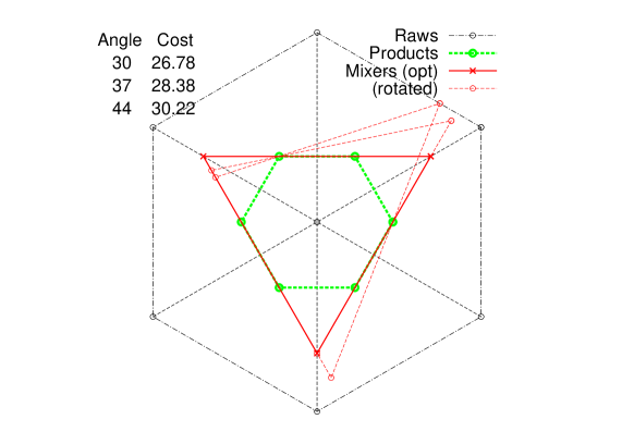
Figure 2: Optimal and forced rotations

Consider first the case where no straights are used. To be feasible the convex hull of the bins must contain all the products. The optimization problem can therefore be viewed as finding the bin triangle that contains all the products that is as close to the centre as possible. The solid red triangle in Fig. 2 shown one global optimum. There are another five symmetric global optima with the bin triangles rotated through $60\degree$, however all intermediate positions are worse. Two sub-optimal solutions are shown. These are the best possible configurations where a bin is forced to lie at angles $37\degree$ or $44\degree$. Forcing the rotation forces the average position of the bins to move outwards, so increasing the cost.

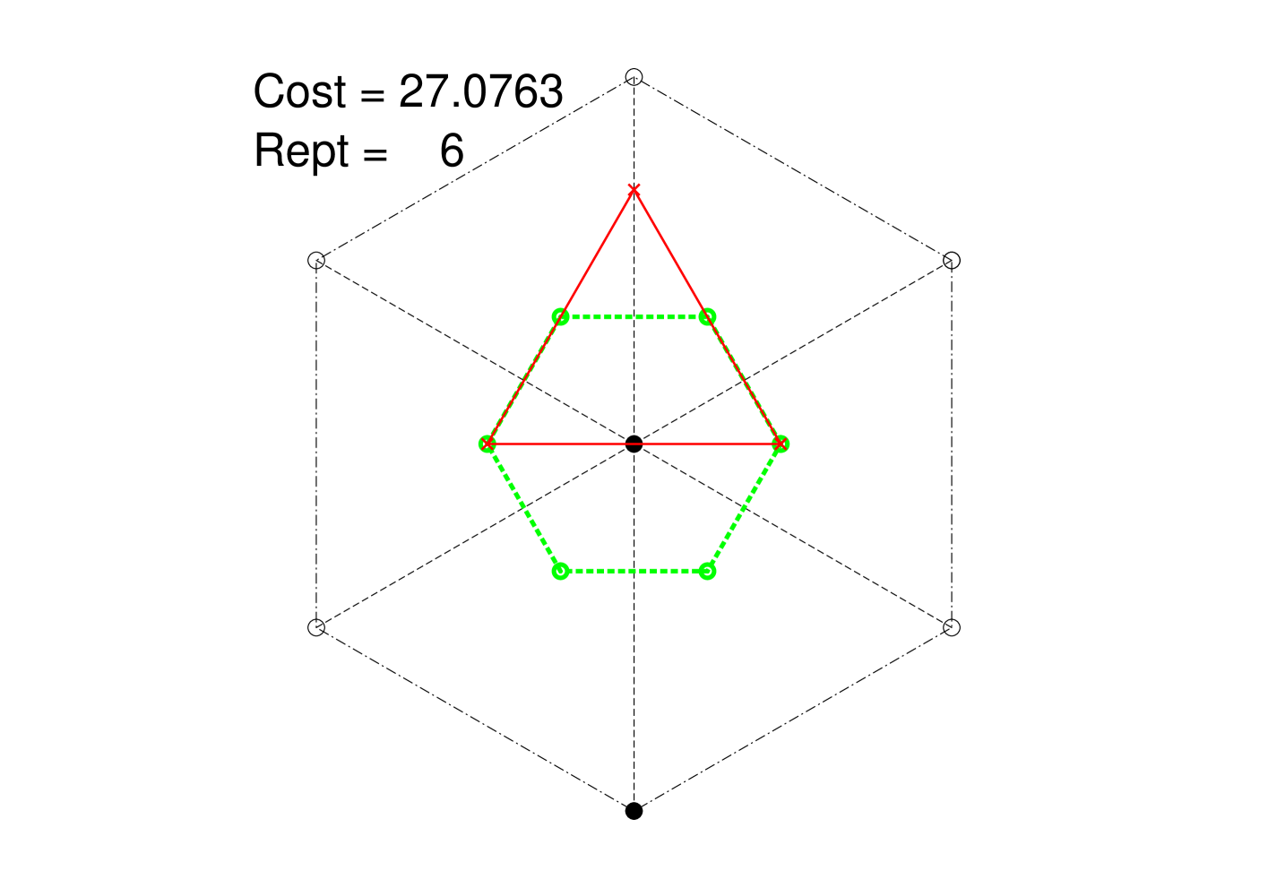
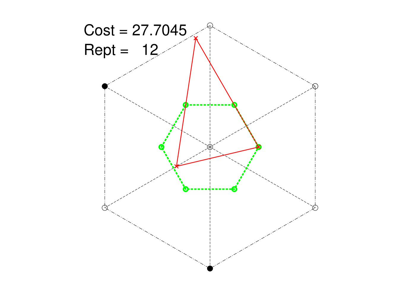
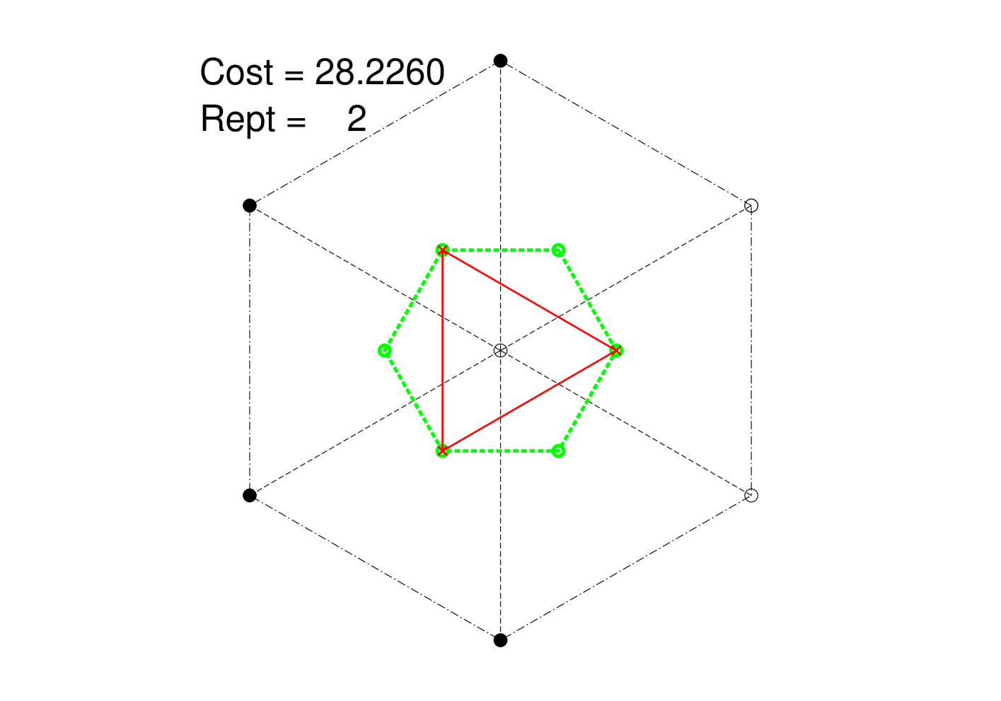
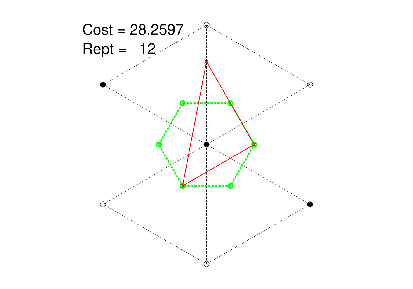
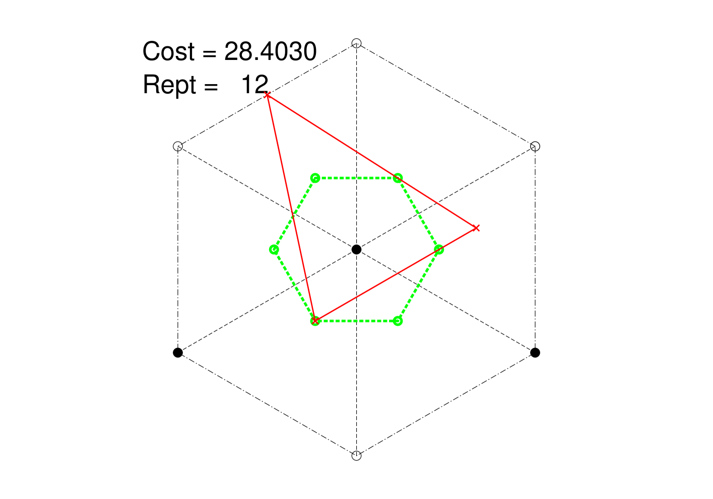
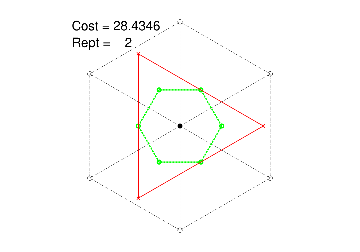
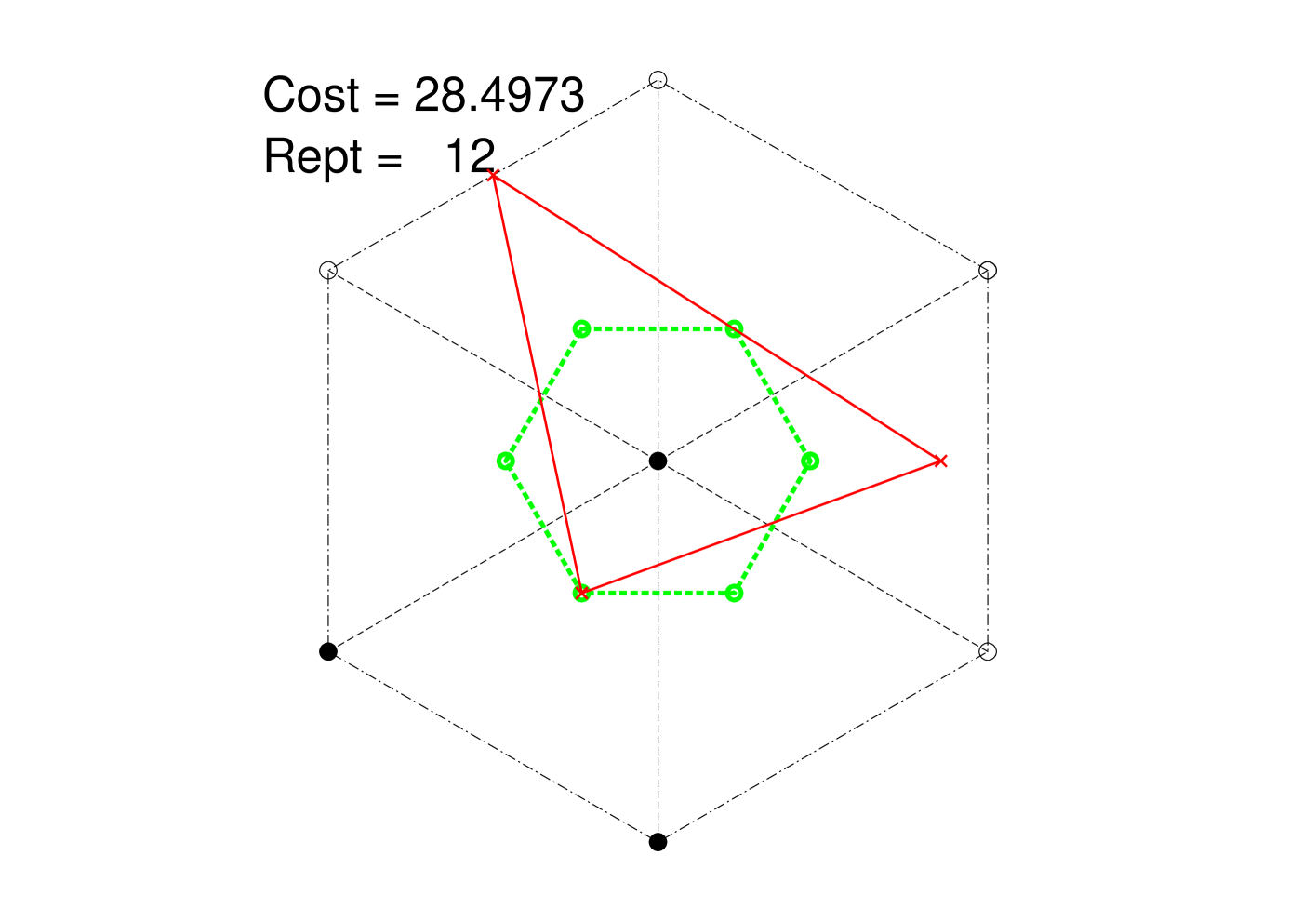
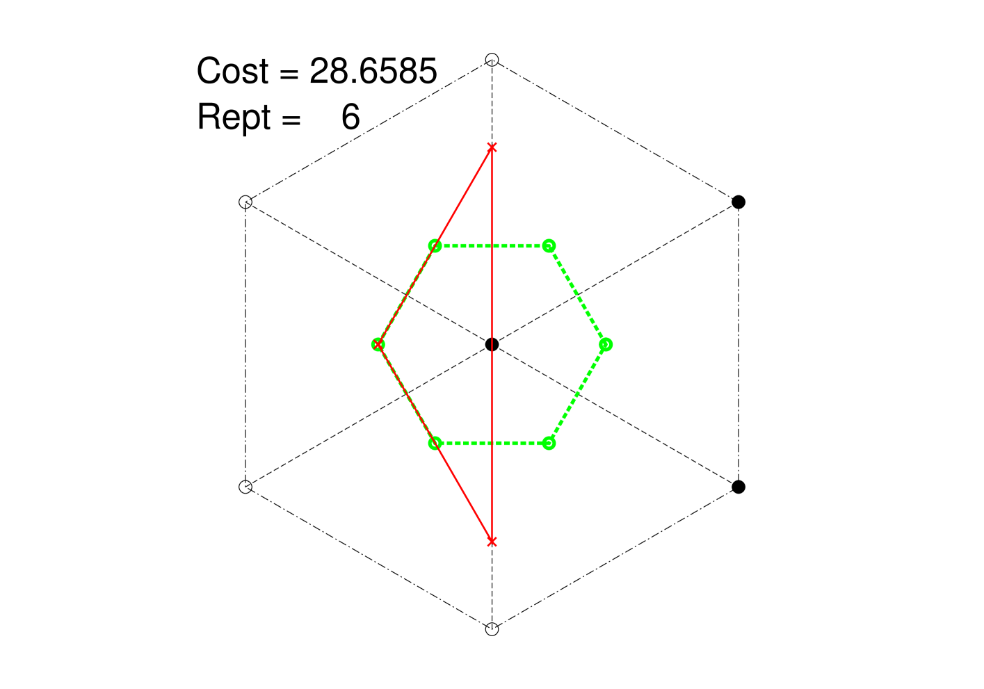
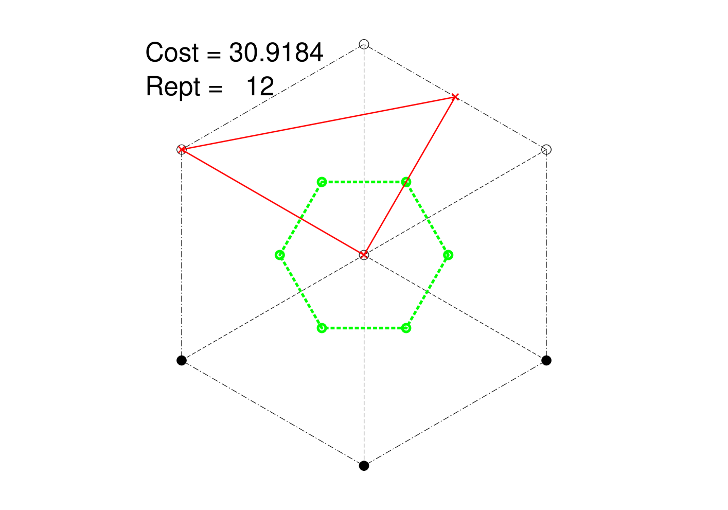
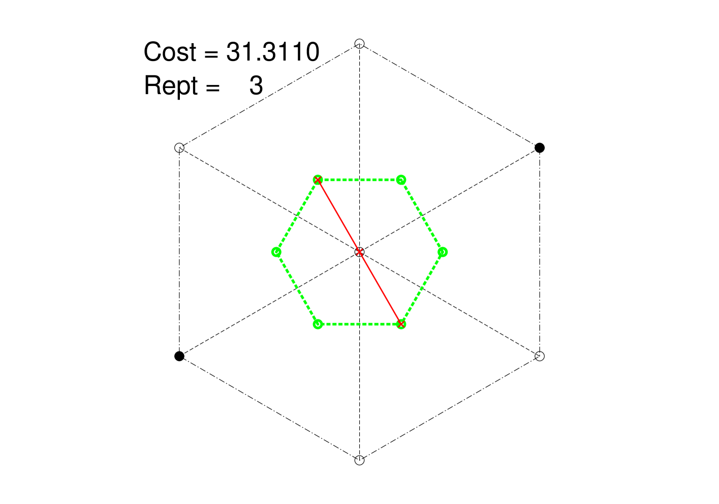
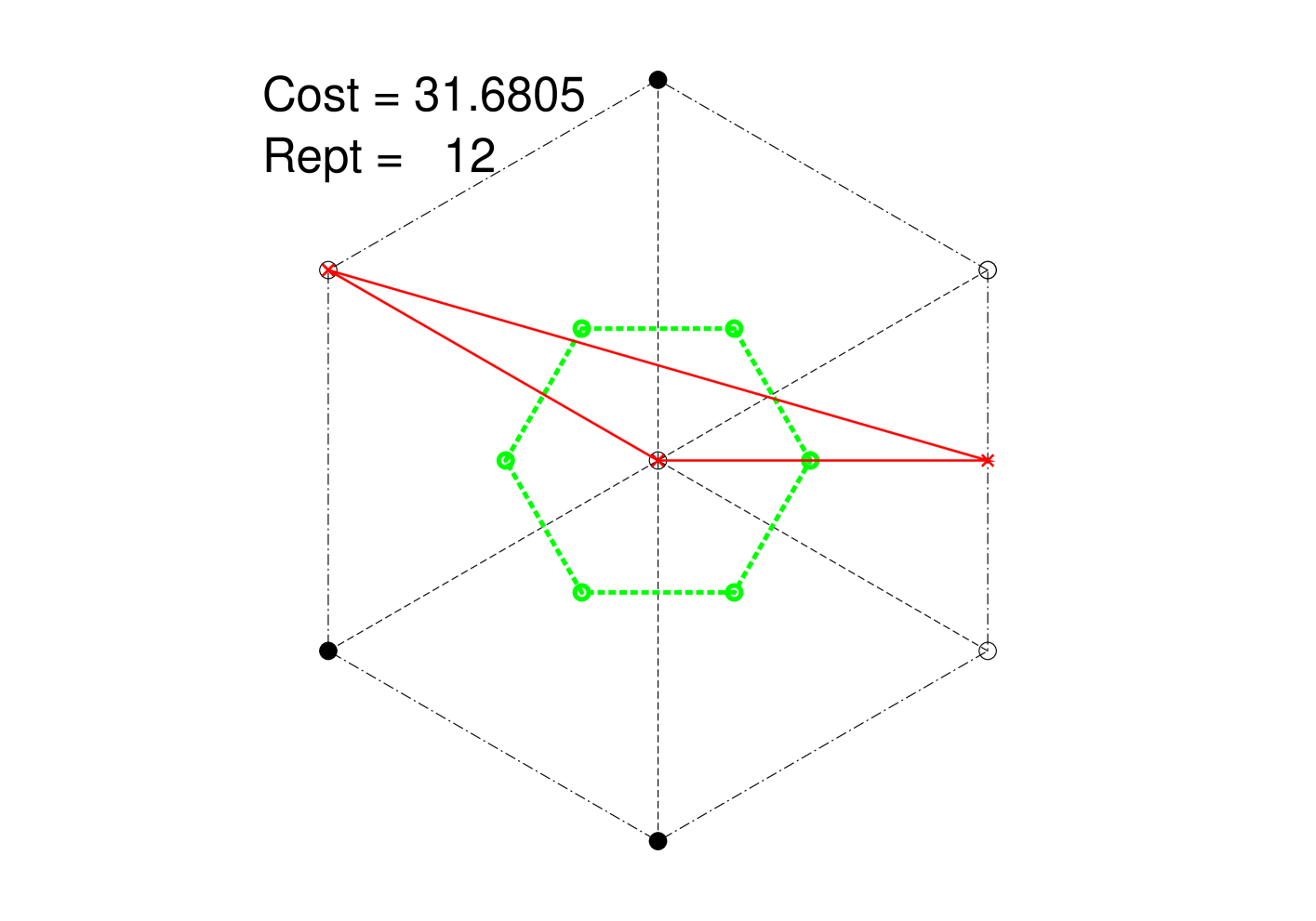
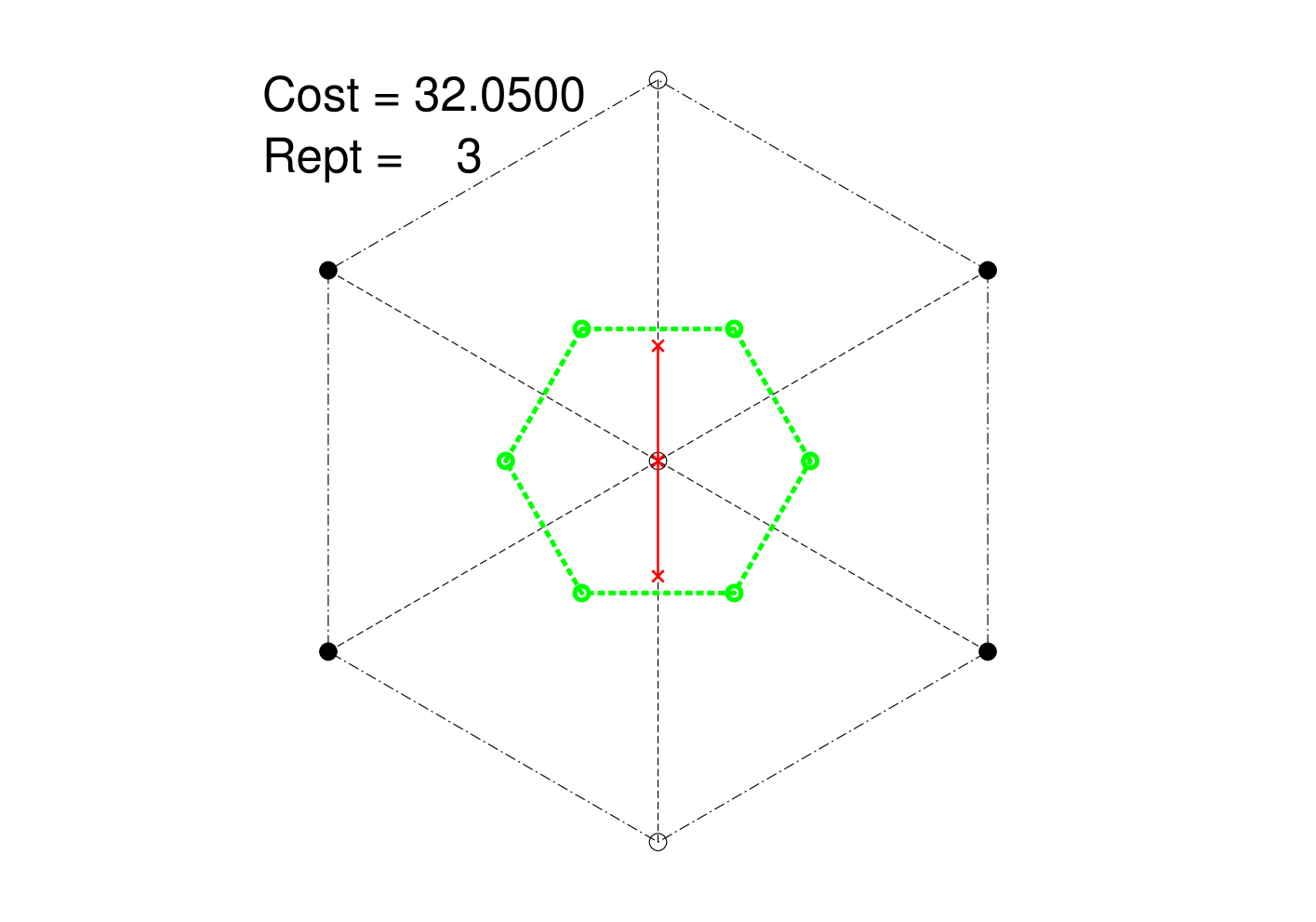
Figure 3: Local Optima: All except the final 4 cases are isolated local optima. The final 4 cases are one example from a 1- or 2-dimensional flat area of local optima.

Now consider the case where it is possible to supply raw materials straight to products without passing thought the mixer bins, but at an extra cost. This removes the need for the convex hull of the bins to contains all the products, and can lead to local optima where the convex hull containing different subsets of the products. Fig 3 shows all the local solutions for the case when the cost of straights is 2.1 time the cost of supply via the bins. We report the cost and the number of repetitions of this solution due to symmetries. When a raw is used as a straight its location is shown with a black dot. In total there are 94 local optimal in addition to the six global solutions in Fig 2. Due to symmetry in the example there are only 13 different values of the cost, but a minor perturbation of the demands or raw material costs would remove this symmetry without destroying the local optimality, and in that case there would be 96 distinct objective values. There is an additional symmetry in the problem as we are assuming all the bins are interchangeable. If this is not the case, for example because the have different capacities or are in different locations with different transport costs, then the number of solutions could increase by a factor of 6.

Finally note that in this example the global solution was the one that did not use any straights. This is due to the relatively high cost of straights. At lower costs this is no longer the optimal solution, and other local solutions become the global one.

4 Solution Methods

The first solution method proposed for the pooling problem was Sequential Linear Programming (SLP) by Lasdon[9]. SLP, as a local method, is not guaranteed to converge to a global minimizer and may even terminate at a local minimum of the corresponding feasibility problem. Even as a local solution method for nonlinear programming problems, SLP has been deemed obsolete due to the development of more sophisticated methods such as Sequential Quadratic Programming (SQP,[5]) and Interior Point Methods (IPM, [14]). Progress made in the implementations of these methods have made the local solution of pooling problems very fast.

More recently advances in dealing with bilinear constraints in MINLP methods [10] within Outer Approximation Branch & Bounds solvers such as Couenne and Baron, have made the global solution pooling problem tractable at least for small instances.

The aim of this study is to evaluate the performance of different local solution methods, namely SQP, SLP and Interior Point using random multistart, and to compare this with a global solution method.

Sequential Linear Programming (SLP).

In order to solve a constrained nonlinear optimization problem

$$\min_{x}f(x),\quad\text{subject to~{}}g(x)\leq 0,$$ (8)

the basic sequential linear programming method uses successive linearizations of the problem around the current solution estimate $x^{(k)}$. That is, given $x^{(k)}$, SLP solves the problem

$$\min_{\Delta x}f(x^{(k)})+\nabla f(x^{(k)})^{T}\Delta x,\quad\text{s.t.~{}}\nabla g(x^{(k)})^{T}\Delta x\leq-g(x^{(k)}).$$ (9)

and then takes a step $x^{k+1}=x^{k}+\Delta x$. Such an iteration will converge to a local solution of the problem only under fortuitous circumstances: even if $x^{(k)}$ is close to the optimal solution, problem (9) may be unbounded or lead to very large steps. In practice the SLP subproblem is therefore wrapped in a Trust Region scheme[3], that is, given a trust region radius $\rho^{(k)}>0$, we solve

$$\min_{\Delta x}f(x^{(k)})+\nabla f(x^{(k)})^{T}\Delta x,\quad\text{s.t.~{}}\nabla g(x^{(k)})^{T}\Delta x\leq-g(x^{(k)}),\|\Delta x\|_{\infty}\leq\rho^{(k)}$$ (10)

and employ the usual Trust Region methodology: that is after every solution we compare the improvement in function value and constraint violation predicted by the linearized model with what can actually be achieved by taking the step $x^{(k)}+\Delta x$. Depending on the outcome of the test we either choose to take the step, that is $x^{(k+1)}=x^{(k)}+\Delta x$ (and possibly enlarge the trust region), or we reject the step, reduce the trust region and keep the same iterate $x^{(k+1)}=x^{(k)}$. Since the test of goodness of the step $\Delta x$ consists of two criteria (objective function and constraint violation) either a merit function or a filter[5] can be employed. In our implementation we are using a filter strategy.

Sequential Quadratic Programming (SQP)

essentially uses the same methodology, but rather than solving the linear approximation (10) it augments this problem by adding the Hessian of the Lagrangian to the problem: that is given a primal-dual estimate $(x^{(k)},\lambda^{(k)})$ of the optimal solution and the constraint multipliers at that point, SQP solves the problem

$$\min_{\Delta x} f(x^{(k)})+\nabla f(x^{(k)})^{T}\Delta x+\tfrac{1}{2}\Delta x^{T}\nabla^{2}_{xx}\mathcal{L}(x,\lambda)\Delta x,$$ (11)

s.t. $$\nabla g(x^{(k)})^{T}\Delta x\leq-g(x^{(k)}),$$

$$\|\Delta x\|_{\infty}\leq\rho^{(k)}$$

where $\mathcal{L}(x,\lambda)=f(x)-\sum_{i=1}^{m}\lambda_{i}g_{i}(x)$ is the Lagrangian function of problem (8).

The second order term can be motivated by realising that the step calculated by (11), without the trust region constraint is the same step that would be calculated by Newton’s Method employed to find a stationary point of the Lagrangian $\mathcal{L}(x,\lambda)$. See for example [5] for further details on the implementation of an SQP method.

5 Results

To evaluate the efficiency of the various problem formulations and solution methods we have tested them on a set of problems taken from the animal feed mix industry.

We have used compared four different formulations, namely the standard pq-formulation (pq), the pq-formulations including the simplifications due to fixed demands (pqs), the qq-formulation (qq) and the qq-formulation strengthened with the pq-equivalent cuts (6b) (qq+). The solvers that we have compared are Baron as a global solver and our own implementation of SLP, FilterSQP[5] and IPOpt (as an Interior Point Method).

Our test problems and their sizes are summarised in Table 1. These are problem instances from industrial practice. In most problems only a subset of the raw materials can be used as straights (i.e. directly feeding into the products). The variants with names ending on ‘fs’, however, allow the full set of straights (at a cost of $10\times$ the normal raw material cost). The problem set is available for download from[6]. The final two columns in Table 1 give the best objective value that has been found by any method in our tests and the best lower bound found by Baron, within 2h of computation time, for any of the tested formulations. Note that for none of the problems and formulations was Baron able to prove optimality. For the strengthened formulations (pq, pqs, qq+) the gap was between 0.1% (af-7b-fs) and 4.5% (af-6), but was between 59% up to 100% (lower bound of $0$) for formulation qq.

problem	N	I	M	P	S	n	m	best known obj	best LB	gap
af-1	8	16	6	25	16	925	310	296.44604	295.93153	0.1%
af-2	9	35	7	30	2	871	407	239334.02	235751.11	1.5%
af-3	11	31	7	27	2	819	442	122257.45	120498.73	1.4%
af-4	14	28	6	32	4	973	608	186097.11	183620.39	1.3%
af-5-fs	17	29	7	18	29	1266	475	119016.92	118763.29	0.2%
af-5	17	29	7	18	5	816	475	124003.48	123243.60	0.6%
af-6-fs	17	31	7	40	31	2555	893	2921.30	2881.41	1.4%
af-6	17	31	7	40	4	1402	893	3074.23	2937.68	4.5%
af-7b-fs	14	35	14	50	35	3788	1024	130290.06	130147.66	0.1%
af-7	14	35	7	50	8	1690	912	151381.81	145928.01	3.6%
af-7b	14	35	14	50	8	2334	1024	147285.00	145928.01	0.9%

Table 1: Test problem statistics: N=#nutrients/qualities, I=#raw materials/inputs, M=#mixing bins/pools, P=#products/outputs, S=#straights (inputs that are allowed to feed directly to outputs), n, m = #variables and constraints in the qq-formulation.

5.1 Local Solvers: SLP, SQP and Interior Point

To compare the different solution algorithms we start with the local solvers: namely SLP, SQP and Interior Point. We have used the qq-formulation for all these runs since it was observed to perform best.

As the Interior Point solvers in these comparisons we have used IPOpt[13], for SQP we have used FilterSQP[5] and our own implementation of a filter-SLP algorithm. FilterSQP uses the active set solver bqpd[4] as the QP solver, whereas SLP uses CPLEX (primal Simplex, which was found to work best in this setting) as the LP solver. Both of these employ LP/QP hotstarts between SLP/SQP iterations and a pre-solve phase that performs bound tightening and scaling of variables. Although bqpd uses a sparse linear algebra implementation, CPLEX is significantly faster than bqpd when both are used to solve the same LP. In order to give a fair comparison of SLP against SQP independent of the subproblem solver used we have in fact tested three SLP/SQP solvers: FilterSQP, FilterSQP as an SLP solver (by simply passing it zero Hessians), and SLP-CPLEX. Apart from the different LP solvers, SLP-CPLEX when compared to FilterSQP without Hessians uses a more aggressive trust region logic and the removal of all features that make use of Hessian information (such as second order correction steps). As we show below, even the ad-hoc SLP setup in FilterSQP-noHess shows some of the advantages of SLP vs SQP, whereas SLP-CPLEX is significantly better than either of them.

As tests were perfomed on a Scientific Linux 7 system using a Intel Xeon E5-2670 CPU running at 2.60GHz. All solvers used only a single thread.

Table 2 shows results from 500 runs of FilterSQP with Hessians (SQP-withHess), FilterSQP without Hessians (SQP-noHess) and our SLP implementation (SLP-CPLEX). Solutions are counted as feasible if the point at which the algorithm stops has a constraint violation of $<10^{-6}$, independent of the status returned by the solver. Column ‘Ti’ shows the average solution time per run, column ‘It’ the average number of SQP or SLP iterations per run and column ‘%Good’ gives the percentage of solutions that are feasible and whose objective value is within $0.2\%$ of the best know solution from any method (which is an acceptable tolerance in practice).

A direct comparison if SQP with either of the two SLP variants is shown in Table 3. The arrows indicate if larger or smaller numbers indicate better results. For columns ‘Ti’, ‘It’ and ‘Ti/It’ we give the value for the SLP variants as a percentage of the corresponding value for SQP-withHess. Column ‘%Good’ gives the percentage point difference of good solutions found between the solvers (positive numbers indicating that SLP found more good solutions, negative numbers show an advantage of SQP). Generally the quality of the solutions found by the SLP variants (SQP-noHessian and SLP-CPLEX) are better than SQP-withHess: the percentage of runs that are within a tolerance of 0.2% of the the best know is on average 4.7% and 18.5% higher for SQP-noHess and SLP-CPLEX respectively. The solution times per run are also better, significantly so in the case of SLP-CPLEX.

The improvements in time per run are due both to a reduction in the number of SQP or SLP iterations and in the time per iteration. On average SQP-noHess and SLP-CPLEX take 55.2% and 3.8% of the SQP-noHess time. This can be accounted for by the time per iteration being significantly less (64.1% and 11.6%), and also because the number of iterations is less (93% and 35%). SQP-withHess and SQP-noHess use the same solver, bqpd, and the reduction in time is due to LP iterations being faster than QP iterations. The further big reduction in time per iteration achieved by SLP-CPLEX is due to the faster LP implementation in CPLEX compared to bqpd. A more surprising reason for the improved time per run is the fact that SQP-noHess and SLP-CPLEX take fewer iterations than SQP-withHess (average 93% and 35% respectively). Intuitively SQP would be expected to be superior to SLP: after all it uses a higher order approximation of the nonlinear programming problem at each iteration. As one (but not the only) consequence SQP displays second order convergence inherited from Newton’s method once it has reached a point close enough to the solution. SLP methods on the other hand may have to resort to reducing the trust region radius to zero after many steps being rejected by the filter in order to terminate. This results in SLP often taking more iterations than SQP to converge to high accuracy.

We do observer this tail effect in our experiments, but note that due to LP hotstarts these iterations are very fast, often requiring only 1 or even 0 simplex basis updates. A larger effect, however, is that away from the neighbourhood of the solution SQP is observed to repeatedly enter the restoration phase before the algorithm is able to “home in” on a solution, and this results in both a higher iteration count and a decreased likelihood of finding a feasible solution than with SLP.

	SQP-withHess			SQP-noHess			SLP-CPLEX
problem	Ti	%Good	It	Ti	%Good	It	Ti	%Good	It
af-1	6.6	66.4	64.9	3.9	81.0	42.2	0.5	79.0	38.0
af-2	44.9	2.0	254.5	19.2	13.2	202.2	1.3	19.4	58.7
af-3	20.6	11.4	105.6	8.0	6.0	111.6	1.3	20.0	50.6
af-4	42.3	12.2	127.4	30.2	10.0	100.7	1.7	19.8	49.1
af-5-fs	145.5	20.2	366.1	26.1	56.0	340.0	1.7	99.6	61.2
af-5	24.2	97.8	106.2	13.2	99.2	151.9	1.5	100.0	53.9
af-6-fs	400.8	0.2	199.5	169.5	0.4	92.7	6.5	5.2	47.0
af-6	112.1	0.0	110.3	87.7	0.0	83.1	4.5	4.0	47.7
af-7b-fs	681.0	0.4	359.0	508.0	0.0	349.0	14.7	52.6	48.5
af-7	99.0	32.6	119.1	58.0	27.2	161.3	4.6	20.4	61.5
af-7b	307.4	27.0	180.1	208.9	33.8	198.2	12.3	71.8	72.0

Table 2: Performance of SQP-withHess, SQP-noHess and SLP-CPLEX:
Average per run: Ti (solution time in sec), It (number of iterations), %Good (percentage of solutions within 0.2% of best known.

	SQP-withHess v SQP-noHess				SQP-withHess v SLP-CPLEX
	Ti$\downarrow$	%Good$\uparrow$	It$\downarrow$	Ti/it$\downarrow$	Ti$\downarrow$	%Good$\uparrow$	It$\downarrow$	Ti/It$\downarrow$
af-1	59.1	14.6	65.0	90.9	7.58	12.6	58.55	12.94
af-2	42.8	11.2	79.4	53.8	2.90	17.4	23.06	12.55
af-3	38.8	-5.4	105.7	36.7	6.31	8.6	47.92	13.17
af-4	71.4	-2.2	79.0	90.3	4.02	7.6	38.54	10.43
af-5-fs	17.9	35.8	92.9	19.3	1.17	79.4	16.72	6.99
af-5	54.5	1.4	143.0	38.1	6.20	2.2	50.75	12.21
af-6-fs	42.3	0.2	46.5	91.0	1.62	5.0	23.56	6.88
af-6	78.2	0.0	75.3	103.8	4.01	4.0	43.25	9.28
af-7b-fs	74.6	-0.4	97.2	76.7	2.16	52.2	13.51	15.98
af-7	58.6	-5.4	135.4	43.3	4.65	-12.2	51.64	9.00
af-7b	68.0	6.8	110.0	61.8	4.00	44.8	39.98	10.01
Average	55.2	4.7	93.1	64.1	3.81	18.5	35.21	10.56

Table 3: Improvements from SQP-withHess to SQP-noHess or SLP-CPLEX:
Ti$\downarrow$, It$\downarrow$ and Ti/It$\downarrow$ are the ratio (as %) of SQP-withHess values to SQP-noHess or SLP-CPLEX values. %Good$\uparrow$ is the difference between the SLP-CPLEX or SQP-noHess quality and the SQP-withHess quality.

As an explanation of this behaviour we offer the following insight: the nonlinearity in the pooling problem is exclusively due to bilinear terms; these give indefinite a Hessian contribution of the form

$$\left[\begin{array}[]{cc}0&1\\ 1&0\end{array}\right].$$

In fact rather than being helpful, these Hessians bias the algorithm towards taking steps along negative curvature directions (increase one bilinear variable while decreasing the other, as much as possible) which is not desirable. Away from the region of quadratic convergence of Newtons method (that is, for the vast majority of the SQP iterations) this can lead to rather erratic behaviour of SQP.

When comparing the two SLP variants, SQP-noHess and SLP-CPLEX, it can be observed that SLP-CPLEX takes significantly fewer iterations and less time to solve each problem, but most noticeably massively increases the likelihood of finding a feasible solution. This does not seem well explained by the algorithmic differences between them. In fact, while the main reason for an infeasible run in the plain SQP algorithm, is convergence to a local solution of the feasibility (phase-I) problem, in the no-Hessian version the main reason for infeasibility is algorithmic failure due to inconsistent second order information – often there are long sequences of rejected second order correction steps that reduce the trust region radius and subsequently lead to premature termination of the algorithm. In SLP-CPLEX this inconsistent algorithm logic has been removed.

	SLP-CPLEX			SQP-withHess			IPOpt
problem	Ti	%Feas	%Good	Ti	%Feas	%Good	Ti	%Feas	%Good
af-1	0.5	100.0	79.0	6.6	80.6	66.4	6.4	96.2	93.2
af-2	1.3	100.0	19.4	44.9	12.6	2.0	30.9	0.0	0.0
af-3	1.3	99.2	20.0	20.6	96.2	11.4	33.9	50.4	33.8
af-4	1.7	98.5	19.8	42.3	56.4	12.2	46.1	53.4	12.8
af-5-fs	1.7	100.0	99.6	145.5	20.6	20.2	58.8	85.0	86.4
af-5	1.5	99.8	100.0	24.2	98.8	97.8	67.3	33.2	33.2
af-6-fs	6.5	95.0	5.2	400.8	15.4	0.2	71.3	99.4	9.6
af-6	4.5	78.4	4.0	112.1	42.8	0.0	37.6	99.4	6.8
af-7b-fs	14.7	99.0	52.6	681.0	22.4	0.4	508.6	58.2	32.0
af-7	4.6	99.0	20.4	99.0	81.0	32.6	82.6	0.0	0.0
af-7b	12.3	98.8	71.8	307.4	72.6	27.0	437.7	2.2	0.6

Table 4: Performance of SLP-CPLEX, SQP-withHess and IPOpt:
Ti (average time per run in sec), %Feas (percentage of runs that are feasible),
%Good (percentage of runs with a solutions within 0.2% of best known) .

Table 4 compares the average solution time of SLP-CPLEX, SQP (with Hessians) and IPOpt. Generally IPOpt takes about the same amount of time as SQP, although with some large variation. In all cases, however, SLP is an order of magnitude faster than either of the other two algorithms. Somewhat surprisingly IPOpt struggles to find feasible solutions for some problems, in particular af-2, af-7  and af-7b where none or almost none of the runs where feasible.

	ETiGood				SLP-CPLEX Speedup relative to:
Problem	SLP-CPLEX	SQP-withHess	IPOpt	Baron	SQP-withHess	IPOpt	Baron
af-1	0.6	9.9	6.9	3	15.7	10.8	4.7
af-2	6.7	2245.0	inf	11	335.0	inf	1.6
af-3	6.5	180.7	100.3	20	27.7	15.4	3.1
af-4	8.6	346.7	360.2	21	40.4	41.9	2.4
af-5-fs	1.7	721.7	68.1	151	422.8	39.9	88.5
af-5	1.5	24.7	202.7	51	16.5	135.1	34.0
af-6-fs	125.0	200400.0	742.7	2331	1603.2	5.9	18.6
af-6	112.5	inf	552.9	147	inf	4.9	1.3
af-7b-fs	27.9	170250.0	1589.4	1362	6091.9	56.9	48.7
af-7	22.5	303.7	inf	268	13.5	inf	11.9
af-7b	17.1	1138.5	72950.0	107	66.5	4258.4	6.2
Average					863.3	507.7	20.1

Table 5: ETiGood is the expected time to find a Good (i.e. 0.2%) solution.
EIiGood = $\mbox{Ti}{100\over\mbox{\%Good}}$ .

Another way to look at the results in Table 4 would be in terms of Expected Time to find a Good solution (ETiGood) which can be worked out as the ratio 100Ti/%Good. These are presented in Table 5. On this measure SLP-CPLEX is significantly faster than the others. The ETiGood speed up of SLP-CPLEX relative to SQP-withHess is in the range 13.5 to 6,091.9 with average 863.3 (excluding the 1 problem where SQP-withHess failed to find a Good solution). The ETiGood speed up of SLP-CPLEX relative to IPOPT is in the range 4.9 to 4,258.4 with average 570.6 (excluding the 2 problem where IPOpt failed to find a Good solution). The ETiGood speed up of SLP-CPLEX relative to Baron is in the range 1.3 to 88.5 with average 20.1.

5.2 Comparison of local and global solvers

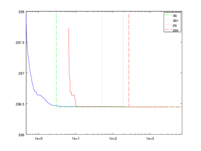
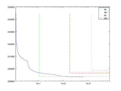
(a)af-1	(b)af-2

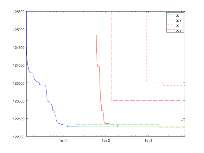
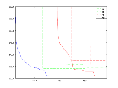
(c)af-3	(d)af-4

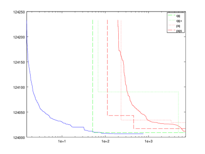
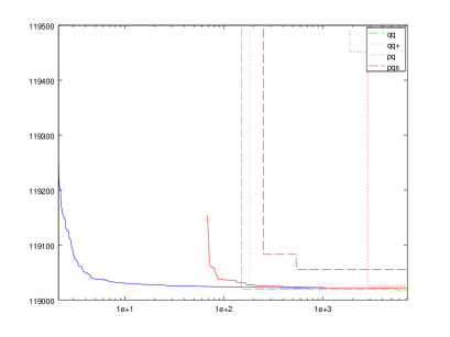
(e)af-5	(f)af-5-fs

Figure 4: Comparing SLP (blue) with IPOpt (red) and Baron for different formulations.

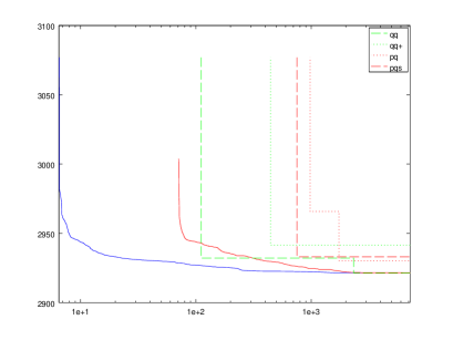
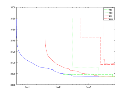
(g)af-6-fs	(h)af-6

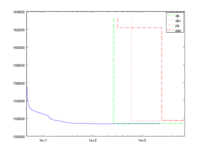
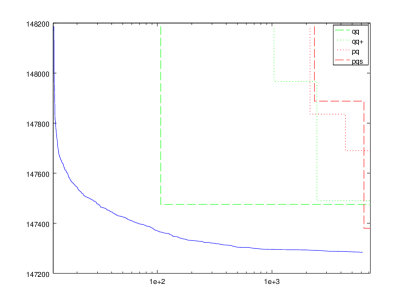
(i)af-7	(j)af-7b

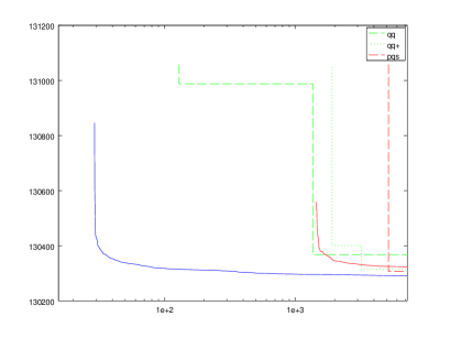
(k)af-7b-fs

Figure 4: Comparing SLP (blue solid) with IPOpt (red solid) and Baron for different formulations (cont).

We have compared the performance of the global solver Baron using the formulations presented in Section 2 with the two best local solvers, namely SLP-CPLEX and IPOpt. Each solve employed a 2 hour time limit for Baron. For the local solvers we have only used the qq-formulation. The results of these experiments are presented in Figure 4.

The graphs should be read as follows: Each gives a plot of quality of solution found ($y$-axis) vs time spend in seconds ($x$-axis, logarithmic). For Baron (for each of the four different formulations) this is a straightforward plot of the progression of the best feasible solution found within the time limit. The lower bounds on the solution obtained are not shown as they are much lower and off the scale of most of the graphs. Indeed the qq+, pq and pqs formulations all obtained the same lower bound (at the root node) that could not be improved within the 2h time limit The qq-formulation leads to significantly weaker lower bounds (gap larger by a factor of 10). The lower bounds are not shown on the graphs since they are (sometimes significantly) below the lower limit of the area shown. Values can be seen in Table 1.

For SLP (blue curve) and IPOpt (red curve) on the qq-formulation we show the expected time that would be needed to obtain a solution at least as good as a given objective value $\hat{v}$. That is let $\bar{t}$ be the average time needed for a local solve. If $k$ out of $n$ SLP/IPOpt runs find a solution better than $\hat{v}$ we model this as a Bernoulli trial with success probability $p=k/n$. The expected number of trials until the first success is $1/p=n/k$ runs or time $\hat{t}=\bar{t}n/k$. From the figures it can be seen that

1. The SLP and IPOpt curves are almost smooth (rather than step functions) indicating that the problems have a huge number of local optima. This ties in with the earlier analysis in Section 3.

2. Baron always finds better solutions with the qq-formulation than with the pq-formulation. The main reason seems to be that the qq-formulation is smaller (since it does not include the pq-constraints) and thus is able to process many more nodes in the same time. In fact the first feasible solution is found by the qq-formulation much faster than for the pq-formulation.

3. Strengthening the qq-formulation by the pq-cut (qq+) does not pay off: neither for the local solvers (due to the larger problem size), nor, somewhat surprisingly, for Baron. While it does strengthen the lower bound, the resulting increase in problem size means that it takes longer to find solutions of the same quality.

4. However, with Baron, the qq-formulation strengthened by the pq-cut (qq+) performs better than the pq-formulation (to which it is in some sense equivalent).

5. SLP is clearly superior to Baron in terms of time taken to find a solution of a given quality: The SLP curve lies well below the Baron curve for almost all problems, times and formulations.

6. Only for the qq-formulation there are a few problems (af-1, af-2, af-6, af-5-fs, af-5) where the first feasible solution found by Baron is better than the best solution that could be expected to be found by SLP in the same time and only for af-2 is the difference more than marginal. However given more time SLP will find a better solution. Also SLP will have already have found very good solutions before Baron with the qq-formulations has found the first feasible solution.

7. At the end of the 2h time limit SLP has always found the best known solution (as given in Table 1). Baron with the qq-formulation fails to find the best solution within 2h for problems af-1, af-5-fs, af-5, af-7b-fs and af-7b.

8. The curve of IPOpt looks similar to the one for SLP but shifted to the right. The reason is that IPOpt needs much longer for a single run ($\overline{t}$) than SLP does. The IPOpt curves seem to drop down quicker than the SLP ones. This is mainly due to the logarithmic scale of the $x$-axis, but also for some problems due to the probability of finding a solution close to globally optimal being larger for IPOpt than for SLP-CPLEX (see Table 4). IPOpt is however clearly uncompetitive for all problems. For problems af-2, af-7 and af-7b the IPOpt curve is not shown (or off the plot) since all (or almost all) of the runs are infeasible.

6 Conclusions

We have given a comparison of several local solvers employing randomized starting points with that of the global solver Baron for the pooling problem.

The best local solver is sequential linear programming, which – while the oldest method – somewhat surprisingly significantly outperforms newer methods such as SQP and Interior Point. Measured by best quality solution obtained in a given time we find that SLP performs much better than Baron for all problem formulations, including the traditional pq-formulation, and almost all time limits. In terms of the expected time to find a solution within 0.2% of the best known SLP with CPLEX as subproblem solver shows an average speedup of respectively 863, 507 and 20 times relative to FilterSQP, IPOpt and Baron.

We further propose a new formulation of the pooling problem, which we term the qq-formulation. This is of comparable size to the q-formulation and can be strengthened by additional cuts analoguous to pq-cuts. When measured as quality of solution found in a given time Baron’s performance on the qq-formulation is superior to all other formulations. However, strengthening this formulation with the pq-like-cuts is not worthwhile on this criterion. The qq-formulation is the only one for which Baron is not totally dominated by SLP for all time limits. With the qq-formulation for a minority of problems the first feasible solution found by Baron is marginally better than the solution that could be expected by randomized SLP in the same time. However for the vast majority of time limits SLP returns better solutions than Baron even for the qq-formulation. One advantage of Baron is that it is able to return a lower bound (and thus an optimality gap), which is not the case for any of the local solvers. However for most of the test examples the bound gap achieved is too large to be of practical value to the problem owner.

References

- [1] Ioannis P Androulakis, Costas D Maranas, and Christodoulos A Floudas. bb: A global optimization method for general constrained nonconvex problems. Journal of Global Optimization, 7(4):337–363, 1995.
- [2] A. Ben-Tal, G. Eiger, and V. Gershovitz. Global minimization by reducing the duality gap. Mathematical Programming, 63:193–212, 1994.
- [3] A. R. Conn, N. I. M. Gould, and P. L. Toint. Trust-Region Methods. MPS-SIAM Series on Optimization, SIAM, Philadelphia, 2000.
- [4] Roger Fletcher. Resolving degeneracy in quadratic programming. Annals of Operations Research, 47:307–334, 1993.
- [5] Roger Fletcher and Sven Leyffer. Nonlinear programming without a penalty function. Mathematical Programming, 91:239–269, 2002.
- [6] A. Grothey and K.I.M. McKinnon. Pooling problem test data. https://www.maths.ed.ac.uk/~agr/PoolingProbs/, 2020.
- [7] Dag Haugland. The computational complexity of the pooling problem. Journal of Global Optimization, 64:199–215, 2016.
- [8] C.A. Haverly. Studies of the behaviour of recursion for the pooling problem. ACM SIGMAP Bulletin, 25:19–28, 1978.
- [9] L.S. Lasdon, A.D. Waren, A. Sarkar, and F. Palacios. Solving the pooling problem using generalized reduced gradient and successive linear programming algorithms. ACM SIGMAP Bulletin, 27, 1979.
- [10] Ruth Misener and Christodoulos A. Floudas. Advances for the pooling problem: Modeling, global optimization, and computational studies survey. Applied and Computational Mathematics, 8:3–23, 2009.
- [11] I. Quesada and I.E. Grossmann. Global optimization of bilinear process networks with multicomponent flows. Computers & Chemical Engineering, 19:1219–1242, 1995.
- [12] M. Tawarmalani and N.V. Sahinidis. Convexification and Global Optimization in Continuous and Mixed- Integer Nonlinear Programming: Theory, Applications, Software, and Applications. Nonconvex Optimization and Its Applications. Kluwer Academic Publishers, 2002.
- [13] A. Wächter and L. T. Biegler. On the implementation of a primal-dual interior point filter line search algorithm for large-scale nonlinear programming. Mathematical Programming, 106:25–57, 2006.
- [14] S. J. Wright. Primal-Dual Interior-Point Methods. SIAM, Philadelphia, 1997.