Combining Learning and Optimization for Transprecision Computing

Abstract

The growing demands of the worldwide IT infrastructure stress the need for reduced power consumption, which is addressed in so-called transprecision computing by improving energy efficiency at the expense of precision. For example, reducing the number of bits for some floating-point operations leads to higher efficiency, but also to a non-linear decrease of the computation accuracy. Depending on the application, small errors can be tolerated, thus allowing to fine-tune the precision of the computation. Finding the optimal precision for all variables in respect of an error bound is a complex task, which is tackled in the literature via heuristics. In this paper, we report on a first attempt to address the problem by combining a Mathematical Programming (MP) model and a Machine Learning (ML) model, following the Empirical Model Learning methodology. The ML model learns the relation between variables precision and the output error; this information is then embedded in the MP focused on minimizing the number of bits. An additional refinement phase is then added to improve the quality of the solution. The experimental results demonstrate an average speedup of 6.5% and a 3% increase in solution quality compared to the state-of-the-art. In addition, experiments on a hardware platform capable of mixed-precision arithmetic (PULPissimo) show the benefits of the proposed approach, with energy savings of around 40% compared to fixed-precision.

1 Introduction

The energy consumption of computing systems keeps growing and, consequently, considerable research efforts aim at finding energy-efficient solutions. A wide class of techniques belongs to the approximate computing[XMK16] field, which has the goal of decreasing the energy associated with computation in exchange for a reduction in the quality of the computation results. In this area, a wide range of techniques have been designed, from specialized HW solutions to SW-based methods[Mit16]. In recent years, a new paradigm called transprecision computing emerged[MSea18, opr], where errors are not merely “tolerated” as byproducts, but rather SW and HW solutions are designed to provide the desired computation quality. Floating-point (FP) operations are a common target for transprecision techniques, as their execution and related data transfers represent a large share of the total energy consumption for many applications involving a wide numerical range[KMBC14, CBB⁺17]. For instance, Tagliavini et al. developed FlexFloat [TMea18], an open-source SW library that allows to specify the number of bits used for the mantissa and the exponent of an FP variable: using a smaller number of bits decreases the precision, thus saving energy.

With the possibility to fine-tune the precision of application variables comes the challenge of finding the best setup. This can be framed as an optimization problem, solvable by paradigms such as Mathematical Programming (MP). The idea is to search for the minimal number of bits that can be assigned to each variable without incurring in a computation error larger than a target. This method requires to analytically express the non-linear relation between precision and the computation error, not a trivial task [MTDM17]. Static analysis of the effect of variables precision is burdensome, and most current approaches have severe limitations[DK17, CBB⁺17]. A possible solution is to learn, rather than directly express, this relation via ML models. We could then embed this knowledge in the optimization model and solve it. This notion is the core idea of Empirical Model Learning (EML)[LMB17], a technique to enable combinatorial optimization over complex real-world systems.

In this paper, we propose a novel optimization method to find optimal variable precision in a transprecision computing setting, based on the EML methodology. The main contributions of this work are:

1. A novel approach, called $SmartFPTuner$, that combines ML models (predicting the error associated with variable precision) and an MP optimization model (finding the optimal precision under a constraint on the error) – this method provides a 55% reduction in solution time w.r.t. state-of-the-art (SoA) tools;

2. An extended model, called $SmartFPTuner^{+}$, that trades off quickness for quality and merges the optimization approach with the SoA algorithm, obtaining a 6.5% speedup over the SoA and a 3% increase in solution quality.

$SmartFPTuner$ enables a significant improvement in execution time that allows integrating this approach into compilation toolchains, but in some cases it produces solutions of lower quality and with marginal energy benefits; $SmartFPTuner^{+}$ bridges this gap, always providing good execution time and high-quality solutions at the same time. Further experiments on PULPissimo, an ultra-low-power platform provided with a mixed-precision HW FP unit, show additional energy savings around 40%.

The rest of the paper is organized as follows. Section 2 discusses the related work in FP precision tuning. Section 3 introduces the proposed approach. Sections 5 and 4 show experimental results on precision tuning and energy efficiency, respectively. Finally, Section 6 provides conclusion and future directions.

2 Related Work

Several works in recent years proposed specific algorithms for FP variable precision tuning [GJea16, RGNea16, GRG18]. The current SoA is the parallel algorithm called fpPrecisionTuning, proposed by Ho et al.[HMWA17]; it is an automated tool that fine-tunes the number of bits to be assigned to FP variables while respecting the constraint on the desired maximum error (for brevity, we refer to this algorithm as FPTuning in the rest of the paper). The algorithm searches for the best solution by running the application to be tuned with different precision levels; a binary search algorithm explores the precision ranges.

Many works have tried to analyze the error introduced by tuning FP variables[RGNea16, MTea17, CBB⁺17]. While promising, these approaches suffer from some limitations: they mostly work at the single-expression level and cannot handle whole benchmarks; those dealing with entire programs (e.g., [RGNea16]) are orders of magnitudes slower than methods such FPTuning; they consider only very few precision levels (e.g., single or double precision).

Finding optimal parameter values for a given algorithm is a well-known area of research. For example, Hutter et al. propose a Sequential Model-based optimization for general Algorithm Configuration (SMAC, [HHLB11]), an automated procedure for algorithm configuration that explores the space of parameter settings. The approach relies on building regression models that describe the relationship between the target algorithm performance and the configuration. Our problem can be cast in the SMAC scheme if we treat the precision of the variables as the algorithm configurations to be explored and the desired target error as a bound on the algorithm performance. We applied SMAC to our problem, but the preliminary attempts were computationally expensive, and the resulting quality lower than problem-specific techniques. Costa et al. developed RBFOpt [CN18], an open-source library for optimization with black-box functions. The method iteratively refines a kernel-based surrogate model of the target function, which is used to guide the search. Our task can be seen as a black-box optimization problem by considering the precision values as the decision variables and the error as the black-box function.

Empirical Model Learning is a relatively new research area, with many potential applications [BLMB12]. We are particularly interested in two specific works, namely: I) Lombardi et al. [BLMB11], which shows how to embed a neural-network-based model in a combinatorial problem, and II) Bonfietti et al. [BLM15], integrating Decision Trees (DT) and Random Forest (RF) models within an MP problem. In our approach, we use their contributions to embed the ML models for predicting the error associated with the variable precision.

3 Proposed Approach

3.1 Problem Description

We consider numerical benchmarks where multiple FP variables take part in the computation of the result for a given input set, which includes a structured set of FP values (typically a vector or a matrix). The number of variables with controllable precision in a benchmark $B$ is $n_{var}^{B}$; these variables are the union of the original variables of the program and the additional variables inserted for handling the intermediate results. For example, if in the original program we have an instruction $V_{1}=V_{2}+V_{3}$ involving three FP variables, the set $B$ contains four FP variables, three corresponding to the $V_{i}$ variables plus the temporary one added to match the precision of the sum before the assignment (i.e., the precision at which the operation is performed). Adopting this approach, each variable is free to contribute to multiple expressions with different precision; practically, HW arithmetic units require operands of the same type, and this requirement can be satisfied with the additional variable.

Our problem consists of assigning a precision to each FP variable while respecting a constraint on the computation error. Assigning a precision means deciding the number of bits for the mantissa; the exponent dictates the extension of dynamic range and is set according to the actual types available on the target HW platform. In the rest of the paper, we refer to the reduction in output quality due to the adjusted precision (reduction w.r.t. the output obtained with maximum precision) as error. If $O$ indicates the result computed with the fine-tuned precision and $O^{M}$ the one obtained with maximum precision, we compute the error $E$ as: $E=\max_{i}\frac{(o_{i}-o_{i}^{M})^{2}}{(o_{i}^{M})^{2}}$ This error metric has been adopted by the current SoA algorithm for precision tuning [HMWA17], and it is one of a broad set of metrics proposed for transprecision computing[MSea18, opr].

In this approach, we focus on the single input set case: we assume a fixed input set to be fed to the benchmark, and we look for the best solution given that precise input set. Consequently, the optimal solution for an input set may not respect the error constraint for other ones. This requirement is not an issue for the comparison with the SoA as it makes the same assumption; our future work aims at overcoming this limitation.

We selected a subset of the applications studied in the context of transprecision computing[opr], chosen because they represent distinct problems and capture different patterns of computation. At this stage, we do not consider whole applications (i.e., training a deep neural net) but we focus on micro-benchmarks that are part of larger applications (i.e., convolution operations, matrix multiplications, etc.). In particular, we chose the following benchmarks:

• FWT, Fast Walsh Transform for real vectors, from the domain of advanced linear algebra ($n_{var}^{FWT}=2$);

• saxpy, a generalized vector addition with the form $y_{i}=a\times x_{i}+y_{i}$, basic linear algebra ($n_{var}^{saxpy}=3$);

• convolution, convolution of a matrix with a $11\times 11$ kernel, ML ($n_{var}^{conv}=4$);

• dwt, Discrete wavelet transform, from signal processing ($n_{var}^{dwt}=7$);

• correlation, compute correlation matrix of input, data mining ($n_{var}^{corr}=7$).

• BScholes, estimates the price for a set of options applying Black-Scholes equation, from computational finance ($n_{var}^{BScholes}=15$);

• Jacobi, Jacobi method to track the evolution of a 2D heat grid, from scientific computing ($n_{var}^{Jacobi}=25$).

We stress out that this is a complex problem, especially the relationship between variable precision and error. First, the error measure is very susceptible to differences between output at maximum precision and output at reduced precision, due to its maximization component. Secondly, the precision-error space is non-smooth, non-linear, non-monotonic, and with many peaks (local optima). In practice, increasing the precision of all variables does not guarantee to reduce the error. This effect is due to multiple factors, such as the impact of rounding operations and the effects of numerical stability on the control flow[DK17]. For instance, suppose to increase only the precision of a variable involved in the condition of an if statement with a constant FP value. Since the modification does not consider this dependence, a rounding of the variable (when its value is near the constant) can trigger different code branches and produce unexpected results on the output.

3.2 Approach Description

We propose an optimization model based on three components: 1) an MP model, 2) an ML model to predict the error associated with a precision configuration, and 3) an ML model to classify configurations in two macro-classes based on the associated error (i.e., small or large). The two ML models are embedded in the MP model and represent the knowledge about the relationship between variables precision and output error.

The MP model finds the optimal bit configuration according to the prediction of the two ML models; to assess the quality of the configuration, we execute the benchmark with the corresponding precision. For this purpose, we employed FlexFloat [TMea18], that allows us to run a benchmark specifying the precision of each FP variable. The task of the ML models is very hard since their goal is to learn a complex function. Hence, the solution found by the MP can be unfeasible; namely, it does not respect the constraint on the target error, due to the gap between estimated and actual error. To fix this problem, we introduce a refinement loop: we test the MP solution by running the benchmark with the specified precision; if the solution is unfeasible, we search for a new one. The wrong one (the configuration plus its actual error) is added to the training set of the ML models, which are then retrained, and cut from the pool of possible solutions of the MP (via a set of constraints). A new MP model is then built based on the refined ML models, and a new search begins; this loop goes on as long as a feasible solution is found. The overall approach is depicted in Figure 1.

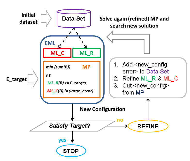
Figure 1: Scheme of the Approach

3.2.1 ML Models

As a first step, we created a collection of data sets containing examples of our benchmarks run at different precision, with the corresponding error values. The configurations used in each data set were obtained via Latin Hypercube Sampling[Ste87], to explore the design space efficiently.

The majority of configurations lead to small errors, from $10^{-1}$ to $10^{-30}$, as the output with fine-tuned variables does not differ drastically from the target one. However, in a minority of cases lowering the precision of critical variables generates errors higher than $100$. Formally, the errors roughly follow a long-tailed distribution: this can be observed by plotting the histogram of the logarithmic error $\log(E)$, as done in Figure 2 for four of our benchmarks. Benchmarks with fewer variables (such as saxpy and conv) have a regular trend, with logarithmic errors always smaller than $0$. When the number of variables increases, for instance with the corr benchmark (green bars), the majority of errors still have a logarithm smaller than $0$; however, we can notice two spikes around $10$ and after $20$. The situation gets even more complicated with BScholes (blue bars); in this case a vast number of configurations correspond to significant errors. This kind of output distribution makes it very difficult for a single model trained in a classical fashion (e.g., for minimum Mean Squared Error) to provide consistently good predictions.

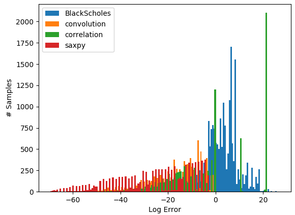
Figure 2: Prediction errors distribution in logarithmic scale

Overly large error values are usually due to numerical issues arising during computation (e.g., overflow, underflow, division by zero, or not-a-number exceptions). This intuitively means that the large-error configurations are likely to follow a distinct pattern w.r.t. the configurations having a lower error value. Accordingly, it makes sense to split the prediction task into two specialized models: a classifier $ML_{C}$ to screen large errors, plus a regressor $ML_{R}$ to evaluate those configurations not ruled-out by the classifier. The $ML_{C}$ needs to make a distinction between normal error and large error configurations. We trained this model by labeling each error in our data set with a class field $c$, equal to $1$ if the error of the example is greater than a threshold ($0.9$ in our experiments), and equal to $0$ otherwise. Configurations classified with class $c=1$ can be discarded by the training set of the regression model.

$ML_{R}$ has the task of predicting the output error for an assignment of precision values. We quickly noticed that any ML model we tried struggled with discerning between small and relatively close errors (i.e., $10^{-20}$ and $10^{-15}$); therefore, we opted to predict the negative of the logarithm of the error, thus magnifying the relative differences and dramatically improving the ML model accuracy. $ML_{C}$ and $ML_{R}$ will be used in the MP model with the aim to, respectively, avoid large-error configurations and enforce the bound on the precision of the variables. Together, the two models offer a more robust prediction, but still not a perfect one.

3.2.2 MP Model

The MP model assigns a precision value to each variable in the benchmark, and it minimizes the total number of bits while respecting the upper bound on the error. We have an integer decision variable $x_{i}^{B},\forall i\in\{1\ldots n_{var}^{B}\}$, namely for each variable of the benchmark. The decision variables represent the number of bits assigned to the variable $x_{i}\in\{nbit_{min}\ldots nbit_{max}\}$. Then we have a continuous variable $e$ that represents the error predicted by $ML_{R}$; as specified earlier, the predicted error is the negative log of the actual error. Finally, we have a variable $c\in\{0,1\}$ which stands for the output of the classifier $ML_{C}$. The decision variables $x_{i}$ and the $e$ and $c$ variables are connected by a set of constraints that encode the $ML_{C}$ and $ML_{R}$ models, generated via the EML library EMLlib.

We then add the constraint that forces the solver not to choose precision values leading to large errors, namely we require $c=0$. We bound the (predicted) error to be below a given target ($E^{target}$, again expressed as log) and then we minimize the total number of bits assigned to the variables:

$$\min z =\sum_{i=1}^{n_{var}^{B}}x_{i}$$ (1)

s.t. $$e\geq E^{target}$$ (2)

s.t. $$c=0$$ (3)

It is important to notice that the constraints described by Equations (1-2) depend on EML methodology, as they encapsulate the empirical knowledge obtained through the ML models. The actual formulation of these constraints has been omitted due to space limitations, as embedding an ML model can require up to hundreds of even thousands of constraints. Nevertheless, the full implementation of the MP model is available on a public code repository . Generally speaking, the number of constraints added due to the embedding of ML models inside MP optimization problems strongly depends on the number of variables in a benchmark, ranging from $38$ in the case of FWT to $4235$ in the case of Jacobi (for an intermediate benchmark such as dwt the number of additional constraints is equal to $513$). We refer to several works already published[BLMB12, LG13, LG16, BLM15] and the publicly available code for details on how ML models can be embedded in MP models as a set of additional constraints.

An additional set of constraints derives from the dependency graph of the benchmark, which specifies how the program variables are related. For instance, consider again the expression $V_{1}=V_{2}+V_{3}$; this corresponds to four precision levels that need to be decided $x_{i},i\in[1,4]$. The first three precision-variables $x_{1}$, $x_{2}$, and $x_{3}$ correspond to the precision of the actual variables of the expression, respectively $V_{1}$, $V_{2}$, and $V_{3}$; the last variable $x_{4}$ is a temporary precision-variable introduced with the FlexFloat API to handle the (possibly) mismatching precision of the operands $V_{2}$ and $V_{3}$ (FlexFloat performs a cast from $x_{2}$ and $x_{3}$ to the intermediate precision $x_{4}$). Each variable is a node in the dependency graph, and the relations among variables are directed edges, as depicted in Fig. 3; an edge entering a node means that the precision of the source-variable is linked to the precision of the destination-variable.

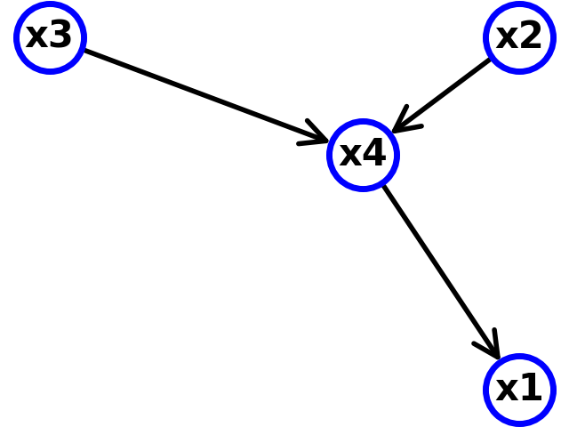
Figure 3: Example of Dependency Graph

From this graph, we can extract additional constraints for the MP model; these constraints greatly prune the search space, thus massively reducing the time needed to find a solution. We focus on two types of relations: I) assignment (e.g., $x_{4}\rightarrow x_{1}$), and II) expression-induced cast (e.g., $x_{2},x_{3}\rightarrow x_{4}$), meaning that the result of an expression involving multiple variables has to converge to the precision associated to the additional variable $x_{4}$.

In assignment expressions, we impose that the precision of the value to be assigned needs to be smaller or equal to the precision of the result, in our example: $x_{4}\leq x_{1}$. Assigning a larger number of bits to the value to be assigned $x_{4}$ would be pointless since the final precision of the expression is ultimately dependent on the precision of the result variable ($x_{1}$). For relations of the second type, we instead bound the additional variable to have a precision equal to the minimum precision of the operands involved in the expression ($x_{4}=min(x_{2},x_{3})$).

4 Experimental Results: Precision Tuning

In this section we provide the implementation of the approach for the selected benchmarks, providing an evaluation of execution time and solution quality.

4.1 ML Models

The current version of the EML library supports two types of ML models, Decision Trees (DT) and Neural Networks (NN): We considered both these techniques in our exploration. The DT and NN models are implemented, respectively, with scikit-learn ML Python module and with Keras and TensorFlow. The NNs are trained with Adam [KB14] optimizer with standard parameters; the number of epochs used in the training phase is 100, and the batch size is 32.

We opted to implement $ML_{R}$ with a NN. After an empirical evaluation, we realized that both NN and DT guaranteed similar prediction errors but with different model complexities: with the NN, few simple layers were needed to reach small errors while good DTs had to be very deep (between 40 and 50 levels). Since the size of a DT (and its encoding) grows exponentially with depth, having so many layers caused issues when constructing the $MP$ model; these issues are solved by the more straightforward structure needed by NN models. Our NN is composed of one input layer (number of neurons equal to $n_{var}^{B}$), three dense hidden layers (with size $2\times n_{var}^{B}$, $2\times n_{var}^{B}$, and $n_{var}^{B}$), and a final output layer of size $1$; all layers employ standard Rectified Linear Units (ReLU), except for the output layer that is linear.

As noted before, we are not interested in having perfect error prediction accuracy in this phase, as $SmartFPTuner$ handles wrong predictions through the refinement phase. Creating a training set needs considerable time, as it requires the execution of multiple configurations. Hence, we use a relatively small training set (1k examples); empirical experiments revealed that more extensive training sets marginally increase the prediction accuracy but not enough to justify the increase in the creation time. The average, normalized error with this training set size and NN is around 8%, though it varies significantly from benchmarks with fewer variables (e.g., 4% for saxpy) to more complex ones (17% for Jacobi).

For $ML_{C}$, after a preliminary evaluation, we settled for using DTs since they provide higher accuracy than NNs even with modest depth ($15$ in our final implementation); averaging on all benchmarks, the $ML_{C}$ accuracy for DT and NN implementations are, respectively, 97% and 82%.

4.1.1 Data set size and prediction error

Since generating the data set used for the ML tasks has non-negligible costs (each benchmark has to be run with many configurations), understanding the impact of the data set size on the prediction error is crucial. Figure 4 shows the effect of the training set size on the prediction error, measured as RMSE (one line for each benchmark). As expected, the error decreases when the training sets contain more examples; however, after a certain size, the gains become marginal (around 4 or 5 thousand examples).

Figure 4: Data set size impact on RMSE

4.1.2 Error Classification

For our classifier, after an empirical evaluation we settled for using a Decision Tree (DT): this proved to reach better accuracy w.r.t. NNs, even with modest depth ($20$ in our final implementation). Table 1 compares the prediction accuracy of DT and NN classifiers (same topology as the regressor one) for different data set sizes. The DTs models neatly outperform NNs, strengthening our conjecture that normal errors and large errors indeed follow different patterns. Furthermore, increasing the training set size does not dramatically improve the performance of the classifier; smaller training sets (around 1000 examples) can be used with good results.

Benchmark	NN					DT
	Data set sizes					Data set sizes
	100	500	1k	2k	8k	100	500	1k	2k	8k
saxpy	1.000	1.000	1.000	1.000	1.000	1.000	1.000	1.000	1.000	1.000
convolution	1.000	1.000	1.000	1.000	1.000	1.000	1.000	1.000	1.000	1.000
FWT	0.850	0.860	0.660	0.677	0.980	0.996	0.997	0.996	0.998	0.998
correlation	0.750	0.790	0.795	0.825	0.962	0.996	0.998	0.995	0.991	0.996
dwt	0.650	0.860	0.930	0.618	0.965	0.991	0.987	0.989	0.992	0.991
BScholes	0.700	0.600	0.675	0.677	0.827	0.983	0.984	0.981	0.985	0.988
Jacobi	0.750	0.810	0.800	0.800	0.836	0.906	0.916	0.919	0.912	0.918
Average	0.740	0.784	0.772	0.719	0.914	0.974	0.976	0.976	0.976	0.978

Table 1: $ML_{C}$ Accuracy Results: DT VS NN

4.2 MP Results

We now examine the solutions found by$SmartFPTuner$. All the experiments were performed using a quad-core processor (Intel i7-5500U CPU 2.40 GHz) with 16 GB of RAM. The MP model was solved using IBM ILOG CPLEX 12.8.0, via the Python API.

4.2.1 Comparison with the State-of-the-Art

We compare our approach with the SoA technique for our problem, the FPTuning algorithm. FPTuning proceeds by testing several precision configurations via binary search; the algorithm is highly parallelized and leads to solutions which are very close to the optimal one, but it has a considerable drawback, namely it has to run the benchmark multiple times to find a feasible solution (we can see it as a variant of a generate-and-test method).

We can highlight two main advantages of $SmartFPTuner$. First, it is more flexible compared to a specific algorithm and more expressive, as more sophisticated constraints can be enforced. For instance, we can constrain the precision of the variables to assume values available on real HW implementations (typically, the only allowed values are 16, 32, and 64 bits). Moreover, the MP can be easily extended for architecture-specific optimization (vectorial instruction sets) and for handling more complex objectives (e.g., minimize the number of casting operations). Secondly, once the ML models have been trained and embedded, the MP model can be used multiple times, relying only on the solver without the need to perform additional benchmark runs. For example, this can be exploited to characterize the error/precision Pareto front, whereas FPTuning would need to start ab initio every time. Considering the current limitations of $SmartFPTuner$, it does not always find good solutions compared to FPTuning; on the contrary, the solutions of $SmartFPTuner$ usually have a higher number of bits.

Table 2 provides an overview of the comparison for all benchmarks. The values reported are computed over all error targets considered, namely $10^{-30}$, $10^{-25}$, $10^{-20}$, $10^{-15}$, $10^{-10}$, $10^{-7}$, $10^{-5}$, $10^{-3}$, $10^{-1}$. Each column from 2-6 corresponds to a benchmark; the last one on the right is the average on all benchmarks. The first row reports the difference (as a percentage) in solution quality between $SmartFPTuner$ and FPTuning, in terms of the number of bits in the solution; a minus sign indicates that our method outperforms FPTuning. The time required to find a solution by $SmartFPTuner$ includes two components: I) the time needed to create the data set to train the ML models and II) the actual solution time, that is the time required to train and integrate the ML models, solve the MP model and eventually repeat the process in case the solution found does not respect the bound on the error. The second row in Table 2 reports the time difference between $SmartFPTuner$ and FPTuning, computed excluding the time needed to create the training sets; including it would not be fair, as after the data set is created it can be reused multiple times and different error targets (it can be used to train different ML models to be integrated via EML). Definitely, the cost for data set creation becomes negligible over repeated calls of $SmartFPTuner$.

The time required to found solutions by FPTuning varies considerably depending on the error given as a target (tighter bounds require longer times), hence the relative differences reported in Tab. 2 are more effective for comparing the approaches. However, it could be useful to provide some actual numbers to give the order of magnitude. For each benchmark and computed as average among all error targets, the solution time (in seconds) required by FPTuning are the following: FWT $24.3$, saxpy $38.5$, convolution $81.9$, correlation $180.9$, dwt $81.8$, BlackScholes $1512.3$, Jacobi $3409.6$.

	FWT	saxpy	convolution	dwt	correlation	BlackScholes	Jacobi	Avg.
SFPT vs FPT – N. Bits (%)	14.1	-1.0	3.7	22.6	14.7	22.3	29.8	15.2
SFPT vs FPT – Time (%)	-62.4	-14.0	-33.5	53.7	-79.5	-80.2	-65.1	-55.4
SFPT+ vs FPT – N. Bits (%)	4.7	-3.9	0.1	0.7	-1.0	-1.7	-4.7	-3.0
SFPT+ vs FPT – Time (%)	-8.2	9.1	9.1	-5.8	-8.3	-22.6	-18.9	-6.51

Table 2: Comparison between $SmartFPTuner$(SFPT in the table), $SmartFPTuner^{+}$(SFPT+)  and FPTuning (FPT)

Concerning the solution quality, FPTuning outperforms us (except for saxpy), since our solutions have a higher number of bits (15% on average). Conversely, $SmartFPTuner$ is markedly quicker, as attested by the average decrease in solution-time of around 55%.

4.3 Extended Approach: $SmartFPTuner^{+}$

As noted in the previous section, $SmartFPTuner$ is extremely fast but produces low-quality solutions, as, generally speaking, higher numbers of bits lead to greater energy consumption. We decided then to extend our approach by combining our method with FPTuning. FPTuning algorithm can be decomposed into two phases: (i) a search for an initial solution satisfying the error target and (ii) a refinement that iteratively improves the solution (by lowering the precision through a heuristic), until two consecutive solutions have the same total number of bits. We propose an extended approach $SmartFPTuner^{+}$ that exploits FPTuning’s refinement phase to improve the initial solution found by $SmartFPTuner$. In practice, $SmartFPTuner^{+}$ starts from the initial solution quickly found by $SmartFPTuner$ and then improves it by attempting to decrease the precision of the variables with the heuristic algorithm introduced by FPTuning (a variant of binary search).

The final two rows of Table 2 show the results.
The time needed by $SmartFPTuner^{+}$ to find a solution contains an additional component w.r.t. to $SmartFPTuner$, namely the time required to improve the initial solution. $SmartFPTuner^{+}$ remains faster than FPTuning (although the gap is reduced, average speedup of around 6.5%) for all but two benchmarks, which are the ones with low number of variables (saxpy and convolution). These “easier” benchmarks can be quickly run multiple times; thus, the FPTuning approach is less penalizing – with applications with more variables $SmartFPTuner^{+}$ is still significantly faster, an encouraging sign for the extension of our approach to more complex programs. More importantly, $SmartFPTuner^{+}$ also outperforms the SoA in terms of solution quality; the improvement is relatively small (3%), but this is remarkable nonetheless, as experiments performing an exhaustive search on small benchmarks reveal that FPTuning finds solutions very close to the optimal ones.

4.3.1 Transfer Learning

As mentioned before, at the moment we are mainly interested in a preliminary evaluation and the comparison with the SoA, hence we considered a single input set for all previous experiments. But at the same time, we want to hint at an additional benefit that can be obtained with the optimization model w.r.t. FPTuning. Our ML models can learn some of the latent proprieties that characterize the benchmarks (their precision-error function); some of these relationships may hold for different input sets. On the contrary, FPTuning focuses exclusively on the problem at hand. Hence, the solutions found by our approach can be more “robust” for different input sets w.r.t. the FPTuning solutions. In a sense, we want to understand if the solution found for a given input set is transferable to different ones.

We tested this hypothesis in this fashion: I) we generated 30 different input sets for each benchmark; II) we found the best configurations for a fixed input set $S_{i}$ using both $SmartFPTuner$ and FPTuning and for a given error target; III) finally, we run the benchmark with the configuration just found but feeding it with the remaining input sets (hence 29 separate runs), and we checked if the configuration satisfies the error target also for other input sets. For these experiments, we considered $SmartFPTuner$ rather than $SmartFPTuner^{+}$ since the focus is on the solution found by the combination of MP and ML models, without the added “noise” introduced by the heuristic refinement phase of $SmartFPTuner^{+}$ (the FPUtning-inspired improvement over the first solution found by $SmartFPTuner$). The different input sets are vectors of randomly generated numbers. The solutions for our approach were obtained using data sets of training size equal to one thousand. Table 3 reports the results. Each row corresponds to an error target; the final one is the average among all targets. For each benchmark, we compute the percentage of input sets that presented an error lower than the target with the configuration found with $S_{i}$ (excluded from this computation); lower values are preferable since they imply that the configuration for $S_{i}$ is more robust. Blacksholes and Jacobi are not reported for space limitations. Columns FPT and Opt (two for each benchmark) indicate, respectively, the results with FPTuning and with $SmartFPTuner$. The last two columns report the average values computed among all benchmarks.

Target	FWT		saxpy		convolution		dwt		correlation		All Benchmarks
	FPT	Opt	FPT	Opt	FPT	Opt	FPT	Opt	FPT	Opt	FPT	Opt
0.1	10.3	44.8	0	0	17.2	0	62.1	79.3	68.9	10.3	31.7	26.9
$10^{-2}$	17.2	89.6	0	0	72.4	0	65.5	62.1	68.9	13.8	44.8	33.1
$10^{-3}$	41.4	41.4	0	0	0	0	65.5	86.2	68.9	10.3	35.2	27.6
$10^{-5}$	0	3.4	0	0	6.8	24.1	75.9	51.7	79.3	62.1	32.4	28.3
$10^{-7}$	0	65.5	62.1	0	0	17.2	55.2	37.9	10.3	24.1	25.5	28.9
$10^{-10}$	0	0	0	0	0	0	86.2	62.1	0	20.7	17.2	16.6
$10^{-12}$	0	0	0	0	0	27.6	62.1	3.4	3.4	0	13.1	6.2
$10^{-15}$	0	0	0	0	0	0	82.7	44.8	0	17.2	16.5	12.4
$10^{-20}$	0	0	86.2	0	0	0	96.5	68.9	0	0	36.5	13.8
$10^{-25}$	0	0	6.9	0	0	0	7.7	0	24.1	0	7.8	0
Average	6.9	24.5	15.5	0	9.6	6.9	72.4	55.2	32.4	15.9	26.1	19.4

Table 3: Transfer Learning Results

From the table we can see that the “transferability” of the solutions strongly depends on the particular benchmark; for example, convolution solutions are very robust to different input sets, while the contrary happens for dwt. For all benchmarks except FWT, $SmartFPTuner$ is more robust compared to FPTuning; this holds true also if we consider all error targets (bold values in the last two columns highlight the method with the more robust solution for a given target). These observations suggest that our approach is capable of learning part of the underlying patterns that characterize an application and thus can obtain solutions that can be reused on different input sets.

However, we are aware that the case of different input sets should be explored in more detail – this is a preliminary approach that we plan to improve in future works. For example, this issue could be dealt with by training the ML models on multiple samples, representative of the target application; the ML model may optionally output a probability distribution rather than a single prediction.

5 Experimental Results: Energy Efficiency

5.1 Deployment & Setup

Our target platform is PULPissimo, an open-source 32-bit microcontroller based on the RISC-V instruction set architecture (ISA). This platform supports the R32IMFC ISA configuration, featuring extensions for integer multiplication and division (“M”), single-precision FP arithmetic (“F”) and compressed encoding (“C”). The core also includes a smallFloat unit (SFU)[MRT⁺18], which provides a set of non-standard ISA extensions to enable operations on smaller-than-32-bit FP formats. This unit supports two IEEE standard formats, single-precision (binary32) and half-precision (16 bit) ones, and two additional formats, namely binary8 and binary16alt. The first is an 8-bit format with low precision (3-bit mantissa), and the second is an alternative 16-bit format featuring a higher dynamic range (8-bit exponent). The SFU also supports a vectorial ISA extension which makes use of SIMD sub-word parallelism by packing multiple smaller-than-32-bit elements into a single register; this is a key feature to reduce energy consumption since it allows to optimize the circuitry of the HW unit and reduce the memory bandwidth required to transfer data between memory and registers.

The software ecosystem of the PULP project includes a virtual platform and a compiler (based on GCC 7.1). The virtual platform is cycle-accurate and provides detailed execution statistics, including instruction and cycle counters, used to evaluate the energy consumption of the benchmarks. The power numbers have been obtained through simulation of the post-layout design set to 350 MHz using worst-case conditions (1.08 V, 125^∘C), as detailed in [MRT⁺18]. Finally, the compiler provides an extended C/C++ type system to make use of the smallFloat types using additional keywords (float8, float16 and float16alt). The GCC auto-vectorizer has been extended to enable the adoption of the vectorial ISA extension; whenever reduced-precision variables can be used, our benchmarks take great advantage of this feature.

5.2 Experimental Evaluation

The energy savings are measured as the energy obtained by running a benchmark with all single-precision variables (the baseline) over the energy obtained with the mixed-precision configuration found by $SmartFPTuner^{+}$; values higher than $1$ indicate energy gains, as the mixed-precision approach leads to lower energy consumption than the baseline. Table 4 reports the results. Each line corresponds to an error bound, and the last line summarizes the average on all targets; each column reports the energy gain compared to the baseline.

Error Target	FWT	saxpy	convolution	dwt	correlation	BlackScholes	Jacobi	Avg. over all benchmarks
$10^{-1}$	1.00	3.99	1.35	1.00	1.08	1.54.	2.90	1.84
$10^{-2}$	1.00	2.26	1.35.	1.00	1.00	1.52	2.90	1.58
$10^{-3}$	1.00	2.00	1.27	1.00	1.00	1.29	1.74	1.33
$10^{-4}$	1.00	1.90	1.22	1.00	1.00	1.08	1.82	1.29
$10^{-5}$	1.00	2.00	1.22	1.00	1.00	1.06	1.77	1.29
$10^{-6}$	1.00	1.13	1.30	1.00	1.00	1.00	1.78	1.17
$10^{-7}$	1.00	1.00	1.00	1.00	1.00	1.00	1.78	1.11
Avg.	1.00	2.04	1.25	1.00	1.00	1.21	2.09	1.37

Table 4: Energy gains measured as energy consumed with single-precision over energy with $SmartFPTuner^{+}$

Overall, the results are extremely promising: the average energy gain obtained with $SmartFPTuner^{+}$ is 1.37 (around 40%), and in the benchmarks showing energy savings the compiler was able to apply automatic vectorization to the code thanks to the precision-reduction enabled by our tool. However, the gains are not homogeneous, as for some benchmarks there is no energy saving w.r.t. the baseline (FWT, dwt, correlation); in these cases, the discrete precision levels offered no margin for energy gain – more fine-grained mixed-precision levels could improve this situation and will be investigated in future works. The results clearly show that, as expected, less strict bounds on the computation accuracy can ensure higher gains since in these cases the variable precision can be reduced more markedly.

6 Conclusion

In this paper we propose a novel approach for solving the problem of tuning the precision of FP variables in numerical applications. Our method combines ML models and an MP optimization model, exploiting the Empirical Model Learning paradigm. The experimental results reveal that the proposed model is very fast but, generally speaking, produces low-quality solutions. Hence we combine our method with a refinement algorithm from the literature, thus obtaining an approach that thoroughly outperforms the SoA.

Moreover, we demonstrate the quality of our approach by measuring the energy gains obtained via static precision tuning on a virtual platform that emulates precision-tunable HW, revealing energy savings around 40% with the static tuning of FP variables.

Acknowledgements

This work has been partially supported by European H2020 FET project OPRECOMP (g.a. 732631).

References

- [BLM15] Alessio Bonfietti, Michele Lombardi, and Michela Milano. Embedding decision trees and random forests in constraint programming. In Proceedings of CPAIOR, pages 74–90, 2015.
- [BLMB11] Andrea Bartolini, Michele Lombardi, Michela Milano, and Luca Benini. Neuron constraints to model complex real-world problems. In Proceedings of CP, pages 115–129, 2011.
- [BLMB12] Andrea Bartolini, Michele Lombardi, Michela Milano, and Luca Benini. Optimization and controlled systems: A case study on thermal aware workload dispatching. In Proceedings AAAI, 2012.
- [CBB+17] Wei-Fan Chiang, Mark Baranowski, Ian Briggs, Alexey Solovyev, Ganesh Gopalakrishnan, and Zvonimir Rakamarić. Rigorous floating-point mixed-precision tuning. ACM SIGPLAN Notices, 52(1):300–315, 2017.
- [CN18] Alberto Costa and Giacomo Nannicini. Rbfopt: an open-source library for black-box optimization with costly function evaluations. Mathematical Programming Computation, 10(4):597–629, 2018.
- [DK17] Eva Darulova and Viktor Kuncak. Towards a compiler for reals. ACM Trans. Program. Lang. Syst., 39(2):8:1–8:28, March 2017.
- [GJea16] Stef Graillat, Fabienne Jézéquel, and et al. Promise: floating-point precision tuning with stochastic arithmetic. In Proceedings of the 17th International Symposium on Scientific Computing, Computer Arithmetics and Verified Numerics (SCAN), pages 98–99, 2016.
- [GRG18] Hui Guo and Cindy Rubio-González. Exploiting community structure for floating-point precision tuning. In Proceedings of the 27th ACM SIGSOFT International Symposium on Software Testing and Analysis, pages 333–343. ACM, 2018.
- [HHLB11] Frank Hutter, Holger H Hoos, and Kevin Leyton-Brown. Sequential model-based optimization for general algorithm configuration. In International Conference on Learning and Intelligent Optimization, pages 507–523. Springer, 2011.
- [HMWA17] Nhut-Minh Ho, Elavarasi Manogaran, Weng-Fai Wong, and Asha Anoosheh. Efficient floating point precision tuning for approximate computing. In Design Automation Conference (ASP-DAC), 2017 22nd Asia and South Pacific, pages 63–68. IEEE, 2017.
- [KB14] Diederik P Kingma and Jimmy Ba. Adam: A method for stochastic optimization. arXiv preprint arXiv:1412.6980, 2014.
- [KMBC14] Pavel Klavík, A Cristiano I Malossi, Costas Bekas, and Alessandro Curioni. Changing computing paradigms towards power efficiency. Phil. Trans. R. Soc. A, 372(2018):20130278, 2014.
- [LG13] Michele Lombardi and Stefano Gualandi. A new propagator for two-layer neural networks in empirical model learning. In Proceedings of CP, pages 448–463, 2013.
- [LG16] Michele Lombardi and Stefano Gualandi. A lagrangian propagator for artificial neural networks in constraint programming. Constraints, 21(4):435–462, 2016.
- [LMB17] Michele Lombardi, Michela Milano, and Andrea Bartolini. Empirical decision model learning. Artificial Intelligence, 244:343–367, 2017.
- [Mit16] Sparsh Mittal. A survey of techniques for approximate computing. ACM Computing Surveys (CSUR), 48(4):62, 2016.
- [MRT+18] S. Mach, D. Rossi, G. Tagliavini, A. Marongiu, and L. Benini. A Transprecision Floating-Point Architecture for Energy-Efficient Embedded Computing. In 2018 IEEE International Symposium on Circuits and Systems (ISCAS), pages 1–5. IEEE, 2018.
- [MSea18] A Cristiano I Malossi, Michael Schaffner, and et al. The transprecision computing paradigm: Concept, design, and applications. In Design, Automation & Test in Europe Conference & Exhibition (DATE), 2018, pages 1105–1110. IEEE, 2018.
- [MTDM17] Mariano Moscato, Laura Titolo, Aaron Dutle, and César A Munoz. Automatic estimation of verified floating-point round-off errors via static analysis. In International Conference on Computer Safety, Reliability, and Security, pages 213–229. Springer, 2017.
- [MTea17] Mariano Moscato, Laura Titolo, and et al. Automatic estimation of verified floating-point round-off errors via static analysis. In Stefano Tonetta, Erwin Schoitsch, and Friedemann Bitsch, editors, Computer Safety, Reliability, and Security, pages 213–229, Cham, 2017. Springer International Publishing.
- [opr] Oprecomp - open transprecision computing. http://oprecomp.eu/. Online; accessed 15 May 2019.
- [RGNea16] Cindy Rubio-González, Cuong Nguyen, and et al. Floating-point precision tuning using blame analysis. In Proceedings of the 38th International Conference on Software Engineering, pages 1074–1085. ACM, 2016.
- [Ste87] Michael Stein. Large sample properties of simulations using latin hypercube sampling. Technometrics, 29(2):143–151, 1987.
- [TMea18] Giuseppe Tagliavini, Stefan Mach, and et al. A transprecision floating-point platform for ultra-low power computing. In Design, Automation & Test in Europe Conference & Exhibition (DATE), 2018, pages 1051–1056. IEEE, 2018.
- [XMK16] Qiang Xu, Todd Mytkowicz, and Nam Sung Kim. Approximate computing: A survey. IEEE Design & Test, 33(1):8–22, 2016.