Pre-thermalization in a classical phonon field: slow relaxation of the number of phonons
François Huveneers
Université Paris Dauphine-PSL, CEREMADE,
Place du Maréchal de Tassigny, 75016 Paris, France
huveneers@ceremade.dauphine.frJani Lukkarinen
University of Helsinki,Department of Mathematics and Statistics,
P.O. Box 68, FI-00014 Helsingin yliopisto, Finland
jani.lukkarinen@helsinki.fi
(March 17, 2024)
Abstract
We investigate the emergence of an astonishingly long pre-thermal plateau in a classical phonon field, here a harmonic chain with on-site pinning.
Integrability is broken by a weak anharmonic on-site potential with strength .
In the small limit, the approach to equilibrium of a translation invariant initial state is described by kinetic theory.
However, when the phonon band becomes narrow, we find that the (non-conserved) number of phonons relaxes on much longer time scales than kinetic.
We establish rigorous bounds on the relaxation time, and develop a theory that yields exact predictions for the dissipation rate in the limit .
We compare the theoretical predictions with data from molecular dynamics simulations and find good agreement.
Our work shows how classical systems may exhibit phenomena which at the first glance appear to require quantization.
Introduction —
Thermalization is one of the most commonly encountered physical phenomena and yet, it still remains poorly understood.
Several materials have been found where the approach to equilibrium can be drastically slowed down or even suppressed:
Anderson insulators Anderson (1958),
many-body localized chains Gornyi et al. (2005); Basko et al. (2006),
ergodic systems featuring many-body scars Turner et al. (2018),
quantum glasses Kagan and Maksimov (1984),
Fermi-Pasta-Ulam-Tsingou chains Fermi et al. (1955),
classical non-linear disordered lattices Basko (2011), etc.
Moreover, some systems with otherwise good ergodic properties, may feature extensive pseudo-conserved quantities that relax only on very long time scales
D’Alessio and Polkovnikov (2013); D’Alessio and Rigol (2014); Lazarides et al. (2014); Abanin et al. (2015, 2017a, 2017b); Mori et al. (2016); Sensarma et al. (2010); Vajna et al. (2018); De Roeck and Verreet (2019); Carati and Maiocchi (2012); Giorgilli et al. (2015); Howell et al. (2019).
The period during which this quantity stays approximately conserved provides an example of pre-thermal state,
that may host a lot of fascinating physical phenomena
Else et al. (2017a, 2019, b); Lindner et al. (2017); Martin et al. (2017).
In this letter, we investigate a classical many-body Hamiltonian in the limit ,
where is integrable (a harmonic lattice or free phonon field) and breaks integrability (an on-site anharmonic potential).
If the system is started in a translation invariant state,
its state evolves swiftly to the generalized Gibbs ensemble (GGE), characterized by all the conserved quantities of
Dudnikova, T. V. and Komech, A. I. and Spohn,
H. (2003); Rigol et al. (2007); Vidmar and Rigol (2016); Essler and Fagotti (2016).
Next, according to kinetic theory and the Boltzmann-Peierls equation, it approaches equilibrium in a time with for
Peierls (1929); Spohn (2006a); Mendl et al. (2016); Lukkarinen (2016).
However, if the phonon band is sufficiently narrow, the (non-conserved) number of phonons is preserved by kinetic processes Spohn (2006b); Mendl et al. (2016),
and only a pre-thermal plateau is reached on kinetic time scales.
As our analysis reveals, the proper equilibrium is only reached after a longer time , scaling as for some .
See Fig. 1 for a summary of the above process.
The presence of an almost conserved quantity (or adiabatic invariant) for the Hamiltonian studied in this letter,
has been realized in Carati and Maiocchi (2012); Giorgilli et al. (2015).
Here, we first provide rigorous quantitative bounds on the dissipation of the number of phonons,
see Claims 1 and 2 below.
In addition, we connect them to the slow dissipation of some quantized fields Sensarma et al. (2010); Abanin et al. (2017b),
a phenomenon that seemed to require quantization.
Second, we provide a theory to compute the dissipation rate of the pseudo-conserved quantity, which we are able to back with numerical results.
General predictions for the rate have been derived in Mallayya et al. (2019) for quantum systems,
see also Lenarčič et al. (2018); Lange et al. (2018); Reimann and Dabelow (2019).
However, we notice that our system is classical
and that an extra time-scale is present since relaxation to the pre-thermal plateau involves kinetic processes.
Figure 1: Expected time evolution of a local observable .
Model –
Let the Hamiltonian be given by
(1)
with an even integer (below we focus on ), and a characteristic frequency of the system.
The dynamics is classical: and
where denotes the time derivative of .
Stability imposes and .
The chain is uncoupled for and unpinned for , and we restrict our attention to .
If needed, we may obviously restrict the summation in eq. (1) to for a length ,
and consider the limit only afterwards.
For , the chain is harmonic.
For a pseudo-momentum in the Brillouin zone , let the phonon mode be defined by
(2)
with the dispersion relation
(3)
and with the Fourier transform of , defined by
.
We identify with the number of phonons with pseudo-momentum and we denote
the total number of phonons by .
From the analyticity of in eq. (3), we deduce that is quasi-local, i.e.
where the kernels decay exponentially with .
When , the Hamiltonian (1) can be written as with
and
(4)
with the notations and .
From eq. (4) and the Poisson bracket rule ,
we deduce that is not conserved, i.e. ,
where denotes the Poisson bracket, due to the terms with .
Pseudo-conservation of —
To compute the time-scales on which gets dissipated, let us first assume that the system is quantized,
i.e. that are creation/annihilation operators for bososns.
Later on, we will see how the conclusions carry over to the classical system.
In this case, has integer spectrum.
In the limit , only resonant processes, preserving the bare energy , do effectively destroy the conservation of .
Therefore, in first order in ,
the process of creating two phonons (since is even, it is not possible to create only one phonon) must satisfy the constraints
(5)
where (we will later consider when dealing with higher order processes),
and where the second constraint is taken modulo 1 and stems from translation invariance, cfr. eq. (4).
Since the width of the dispersion relation in (3) scales as for small ,
larger and larger values of are needed to satisfy the constraints in eq. (5).
Thus, for given even, there exists such that eq. (5) only has solutions for :
(exact), (exact), (numerical),
and in general for , see the Supplemental Material (SM).
From now on, we will assume that is such that for any , leaving these exceptional cases for further studies.
Higher order processes need obviously to be taken into account in the case .
The analysis detailed in the SM yields that a process of order
involves the creation/annihilation of phonons111This
value may also be recovered from a simple power counting argument:
Let ( for a quantum system with ) and expand at order ;
this yields which is a polynomial of order in , with as given.,
and the above analysis caries over with this new value for .
Given and , we may now determine the smallest so that a process of order destroys effectively:
is the only integer such that
Table 1: Order of the processes destroying effectively the conservation of , for in eq. (4).
We observe that, even though quantitative statements are obviously model dependent,
and in particular the threshold values depend on the specific form of the dispersion relation in eq. (3),
the conclusion that as is generic (for a polynomial interaction ),
following from the fact that the width of the band in decays as for .
The above analysis may be turned into rigorous results, using the formalism developed in Abanin et al. (2017b)
that can be straightforwardly adapted to a classical system through the canonical replacement by , see SM and below.
The key observation to proceed is that, even though is no longer quantized, the spectrum of is:
Hence, it acts formally in the same way as the quantum super-operator , and this is eventually what matters.
Let us fix and such that , and let us first express a result in a formulation directly inspired from Abanin et al. (2017b):
There exists a canonical change of variables, bringing into , so that ,
where the term is extensive.
To formulate a precise claim, we will consider extensive observables of the form
(7)
where and where is analytic in , ensuring that is a sum of quasi-local observables.
A function will simply be said to be a polynomial (of order )
if it is of the form with as in eq. (7).
The following claim is shown in the SM:
Claim 1
Let be finite and let us assume periodic boundary conditions.
For small enough,
there exists a polynomial ,
such that is a well defined real analytic function in a neighborhood of the origin in ,
and such that ,
where are polynomials and where the expansion converges to an analytic function in a neighborhood of the origin in .
Claim 1 provides a good way to think about the phenomenon but does not yield as such a very powerful result in the thermodynamic limit:
The radius of convergence of may shrink as
(even though we are interested in the regime , the limit needs to be taken before the limit ).
As a way out, we may undo the above transformation to obtain a dressed number of phonons, , and then truncate its expansion at order .
Doing so, we end up with a well defined pseudo-conserved quantity in the thermodynamic limit, see the SM for details:
Claim 2
Let now the chain be defined on the full lattice .
There exists a quantity ,
where are polynomials of order for ,
such that .
These claims furnish upper bounds on the dissipation rate of , but the determination of this rate requires the knowledge of the instantaneous state of the system.
To proceed further, we will invoke additional assumptions, and leave mathematical rigor behind.
Evaluation of the decay rate —
For , .
The dissipation rate of the density in an instantaneous state and in the infinite volume limit is given by ,
with a flux and where ””
stands for the infinite volume, corresponding to in a chain of finite length.
If the system is prepared in a translation invariant state with zero average, after a short transient time,
it evolves towards a GGE characterized by a Wigner function ,
i.e. a Gaussian state .
Usual kinetic theory yields the following expression for the rate :
Given a function , let , then
(8)
where denotes the average over the GGE, and where the dynamics in the time integral is the free dynamics ().
Expression (8) can thus be evaluated explicitly in leading order.
In the SM, we provide a derivation of eq. (8) which is fully consistent with the derivation used in the more general case .
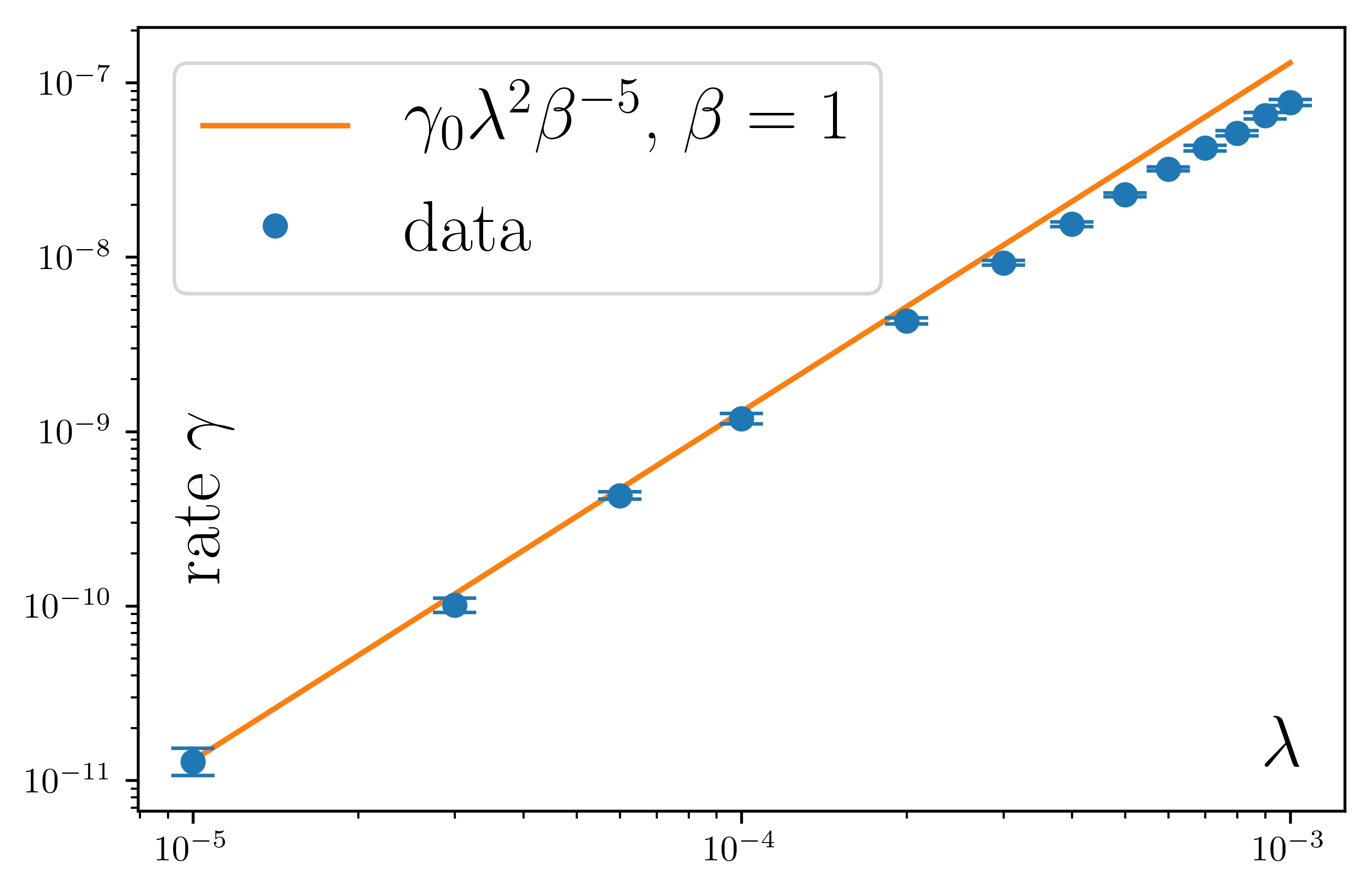
We tested numerically the validity of eq. (8) for and ,
for an out-of-equilibrium initial state corresponding to with and various values of .
We found excellent agreement with the value of extracted from direct simulation of the dynamics,
see Fig. 2.
See SM for the numerical protocol.
Figure 2: as a function of (upper panel) and (lower panel) for and .
Kinetic theory, i.e. eq. (8), predicts with for .
For , we find it convenient to move to the rotated frame where is pseudo-conserved quantity of , see Claim 1.
The GGE is now parametrized by only two extensive quantities and .
Our main assumption (to be discussed later on) is that the system is in a state , -close to the GGE :
(9)
where is some correction that will be determined by maximizing local stationarity.
The key observation is that where Mallayya et al. (2019).
Indeed,
and the integral of a Poisson bracket vanishes.
Hence the instantaneous dissipation rate may be written as
Since this rate scales as , the state itself evolve on that time scale.
Stationarity on shorter time scales determines and an explicit computation yields, see SM:
(10)
Again, the dynamics in the time integral is the dynamics generated by and can thus be computed explicitly in leading order.
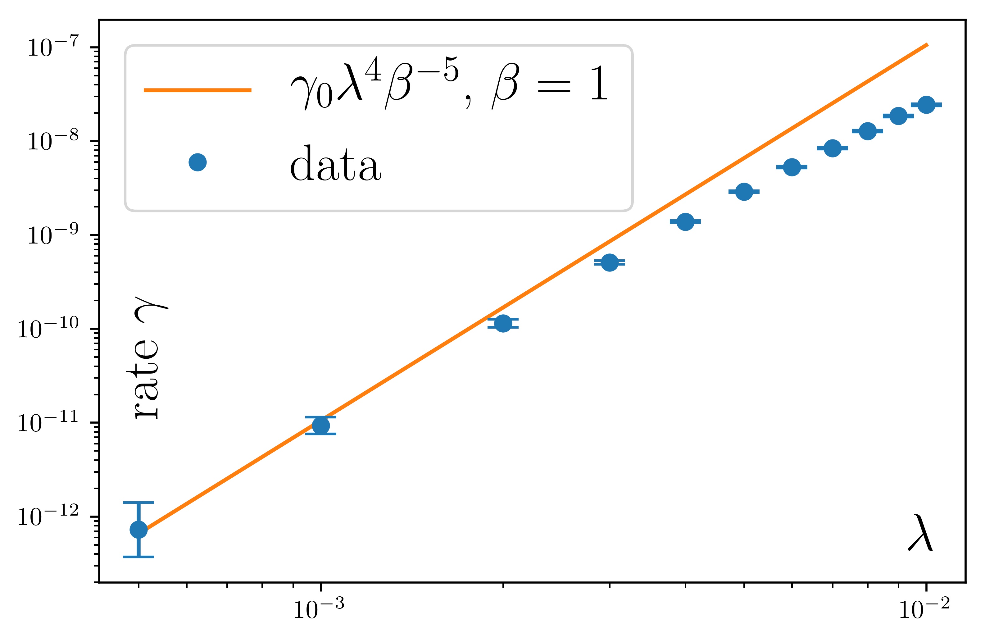
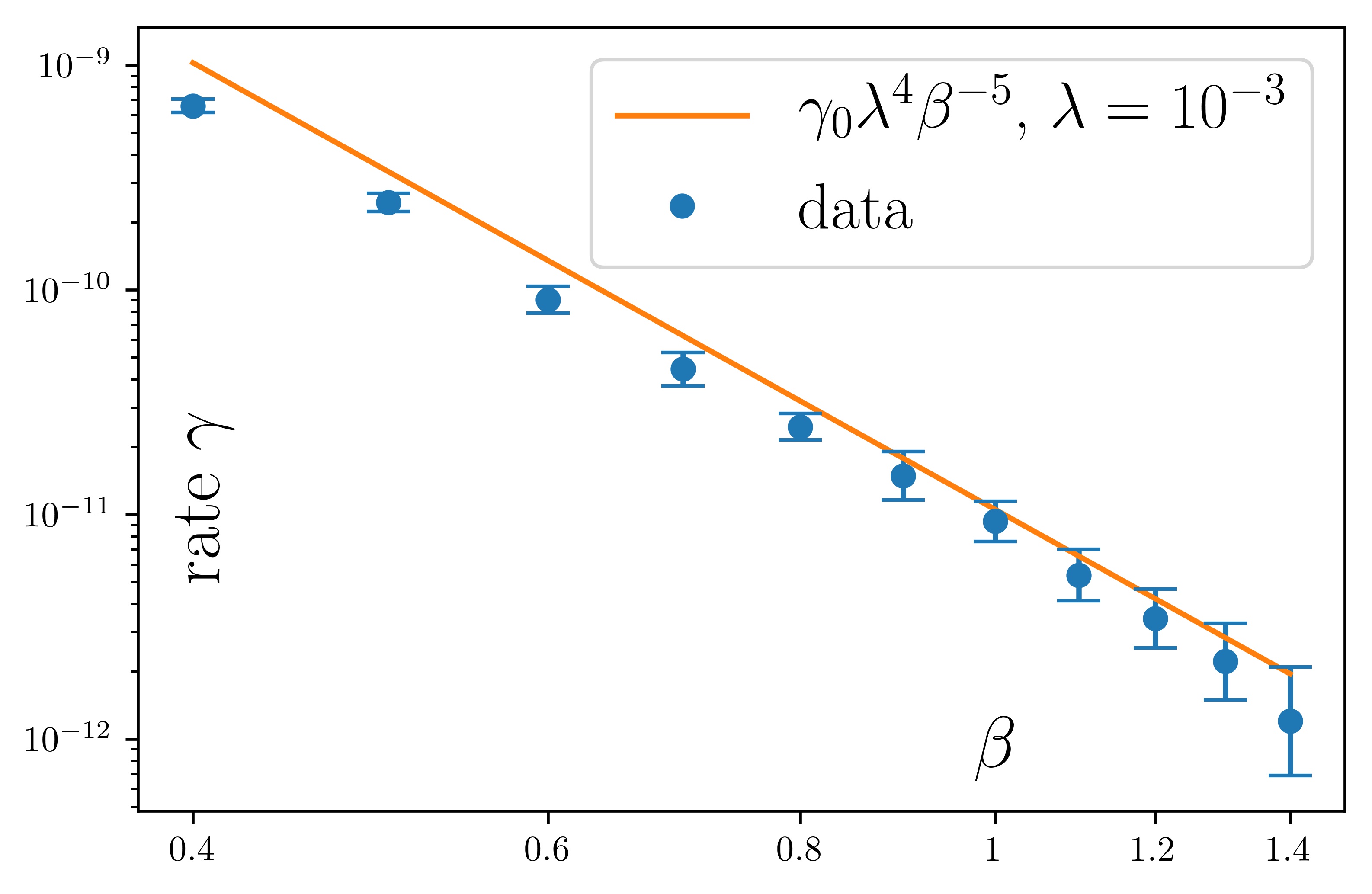
Figure 3: as a function of (upper panel) and (lower panel) for and .
Our theory, eq. (10), predicts with .
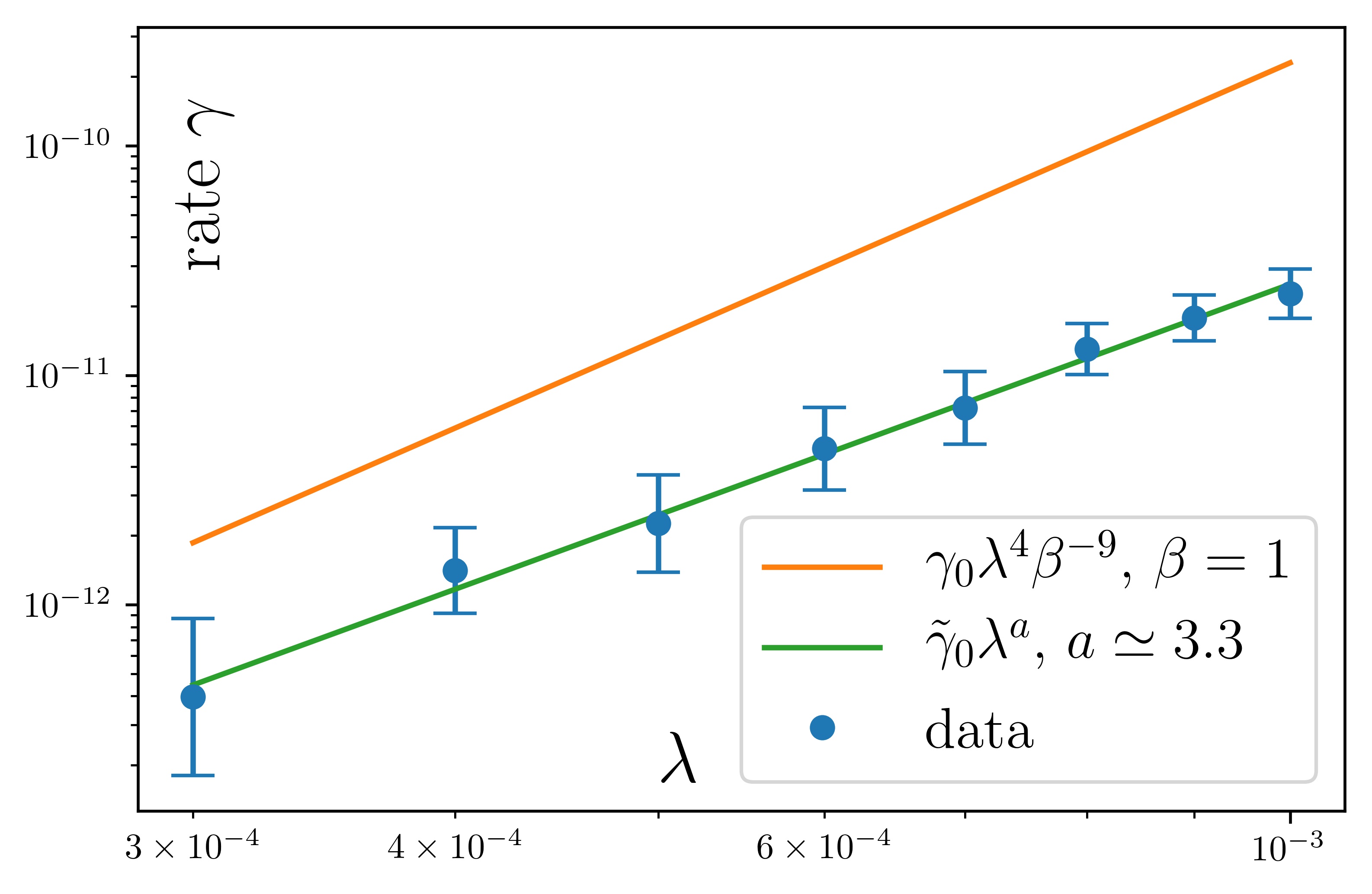
Figure 4: as a function of (upper panel) and (lower panel) for and .
Our theory, eq. (10), predicts with .
We performed two sets of tests in the case
(accessing larger values of would require too long simulation times).
In all cases, we start from a state of the type with and various values of .
For and , the results reported on Fig. 3 show very good agreement between the prediction from eq. (10)
and direct simulation of the dynamics.
For and , the observed rate is significantly smaller than the one predicted by eq. (10),
but it decreases slower as a function of and ,
see Fig. 4.
Comparing with the discrepancies at the largest values of on the upper panel of Fig. 3,
makes it plausible that our theory just needs smaller values of to be validated.
Besides, the fact that the observations are below the theoretical predictions is a second indication that the theory will become accurate for smaller values of ,
since a smaller rate guarantees that our main hypothesis, eq. (9), from which our predictions follow, is more easily satisfied.
Irrespectively of numerical observations, we finally would like to make a consistency check of the main assumption in eq. (9).
On the one hand, due to the dissipation of , the state evolves with time at a rate ,
i.e. evolve at this rate in order to yield correct values for and .
On the other hand, the system relaxes towards the instantaneous pseudo-equilibrium through kinetic processes.
Assuming that the state is at a distance of order from , as required by eq. (9),
we conclude that it moves at a rate .
Consistency of the theory requires that ,
i.e. that the instantaneous fixed point moves slow enough so that the state has the time to relax to it.
Clearly, this is wrong for , marginal for and fine for .
We had treated separately the case , since indeed there is no reason to think that the pre-thermal state should be characterized by the two parameters only.
Unfortunately, the above argument is not conclusive for , while numerical data are only available in this case.
Conclusions and outlook –
Our work provides a new example of long pre-thermal plateau,
it shows how a phenomenology initially explored in quantum systems carries over to a classical set-up,
and it participates to recent efforts to describe accurately the dissipation of pseudo-conserved quantities.
The main features of our theory carry over to and, for ,
we may contemplate the possibility of realizing a pre-thermal Bose-Einstein condensate in this classical system,
exploiting the conservation of the number of phonons over a very long period.
Acknowledgements.
We thank W. De Roeck and H. Spohn for helpful discussions, and C. Mendl for providing the original code for numerical simulations.
F. H. and J. L. benefited from the support of the project EDNHS ANR-14-CE25-0011,
and F. H. from the project LSD ANR-15-CE40-0020-01 of the French National Research Agency (ANR),
as well as from the support of the International Centre for Theoretical Sciences (ICTS) during a visit for the program
- Thermalization, Many body localization and Hydrodynamics (Code: ICTS/hydrodynamics2019/11).
The work has also been supported by the Academy of Finland via the Centre of Excellence in Analysis and Dynamics Research (project 307333)
and the Matter and Materials Profi4 university profiling action.
Gornyi et al. (2005)I. Gornyi, A. Mirlin, and D. Polyakov, “Interacting electrons in
disordered wires: Anderson localization and low-T transport,” Physical Review Letters 95, 206603 (2005).
Basko et al. (2006)D. M. Basko, I. L. Aleiner,
and B. L. Altshuler, “Metal–insulator
transition in a weakly interacting many-electron system with localized
single-particle states,” Annals of Physics 321, 1126–1205 (2006).
Turner et al. (2018)C. J. Turner, A. A. Michailidis, D. A. Abanin, M. Serbyn, and Z. Papic, “Weak ergodicity breaking from quantum
many-body scars,” Nature Physics 14, 745–749 (2018).
Kagan and Maksimov (1984)Y. Kagan and L. Maksimov, “Localization
in a system of interacting particles diffusing in a regular crystal,” Zhurnal
Eksperimental’noi i Teoreticheskoi Fiziki 87, 348–365 (1984).
Fermi et al. (1955)E. Fermi, P. Pasta,
S. Ulam, and M. Tsingou, Studies of the nonlinear problems, Tech. Rep. (Los Alamos Scientific Lab., N.
Mex., 1955).
Basko (2011)D. Basko, “Weak chaos in
the disordered nonlinear Schrödinger chain: destruction of Anderson
localization by Arnold diffusion,” Annals of Physics 326, 1577–1655 (2011).
D’Alessio and Polkovnikov (2013)L. D’Alessio and A. Polkovnikov, “Many-body
energy localization transition in periodically driven systems,” Annals of
Physics 333, 19–33
(2013).
D’Alessio and Rigol (2014)L. D’Alessio and M. Rigol, “Long-time
Behavior of Isolated Periodically Driven Interacting Lattice Systems,” Physical Review X 4, 041048 (2014).
Lazarides et al. (2014)A. Lazarides, A. Das, and R. Moessner, “Equilibrium states of
generic quantum systems subject to periodic driving,” Physical Review E 90, 012110 (2014).
Abanin et al. (2015)D. A. Abanin, W. De Roeck, and F. Huveneers, “Exponentially Slow Heating
in Periodically Driven Many-Body Systems,” Physical Review Letters 115, 256803 (2015).
Abanin et al. (2017a)D. A. Abanin, W. De Roeck,
W. W. Ho, and F. Huveneers, “Effective Hamiltonians, prethermalization, and
slow energy absorption in periodically driven many-body systems,” Physical Review B 95, 014112 (2017a).
Abanin et al. (2017b)D. A. Abanin, W. De Roeck,
W. W. Ho, and F. Huveneers, “A Rigorous Theory of Many-Body
Prethermalization for Periodically Driven and Closed Quantum Systems,” Communications in Mathematical Physics 354, 809–827 (2017b).
Mori et al. (2016)T. Mori, T. Kuwahara, and K. Saito, “Rigorous Bound on Energy Absorption
and Generic Relaxation in Periodically Driven Quantum Systems,” Physical Review Letters 116, 120401 (2016).
Sensarma et al. (2010)R. Sensarma, D. Pekker,
E. Altman, E. Demler, N. Strohmaier, D. Greif, R. Jördens, L. Tarruell, H. Moritz, and T. Esslinger, “Lifetime of double occupancies in the Fermi-Hubbard model,” Physical Review B 82, 224302 (2010).
Vajna et al. (2018)S. Vajna, K. Klobas,
T. Prosen, and A. Polkovnikov, “Replica Resummation of the
Baker-Campbell-Hausdorff Series,” Physical Review Letters 120, 200607 (2018).
De Roeck and Verreet (2019)W. De Roeck and V. Verreet, “Very slow
heating for weakly driven quantum many-body systems,” arXiv (2019), arXiv:1911.01998
[cond-mat.stat-mech] .
Giorgilli et al. (2015)A. Giorgilli, S. Paleari,
and T. Penati, “An extensive adiabatic
invariant for the Klein–Gordon model in the thermodynamic limit,” Annales Henri
Poincaré 16, 897–959 (2015).
Howell et al. (2019)O. Howell, P. Weinberg,
D. Sels, A. Polkovnikov, and M. Bukov, “Asymptotic Prethermalization in Periodically Driven
Classical Spin Chains,” Physical Review Letters 122, 010602 (2019).
Else et al. (2017a)D. V. Else, B. Bauer, and C. Nayak, “Prethermal Phases of Matter Protected
by Time-Translation Symmetry,” Physical Review X 7, 011026 (2017a).
Else et al. (2019)D. V. Else, W. W Ho, and P. T. Dumitrescu, “Long-lived interacting
phases of matter protected by multiple time-translation symmetries in
quasiperiodically-driven systems,” arXiv (2019), arXiv:1910.03584 [cond-mat.str-el]
.
Else et al. (2017b)D. V. Else, P. Fendley,
J. Kemp, and C. Nayak, “Prethermal Strong Zero Modes and Topological
Qubits,” Physical Review X 7, 041062 (2017b).
Lindner et al. (2017)N. H. Lindner, E. Berg, and M. S. Rudner, “Universal chiral quasisteady
states in periodically driven many-body systems,” Physical Review X 7, 011018 (2017).
Martin et al. (2017)I. Martin, G. Refael, and B. Halperin, “Topological Frequency
Conversion in Strongly Driven Quantum Systems,” Physical Review X 7, 041008 (2017).
Rigol et al. (2007)M. Rigol, V. Dunjko,
V. Yurovsky, and M. Olshanii, “Relaxation in a Completely Integrable
Many-Body Quantum System: An Ab Initio Study of the Dynamics of the Highly
Excited States of 1D Lattice Hard-Core Bosons,” Physical Review Letters 98, 050405 (2007).
Mendl et al. (2016)C. B. Mendl, J. Lu, and J. Lukkarinen, “Thermalization of oscillator chains
with onsite anharmonicity and comparison with kinetic theory,” Physical Review E 94, 062104 (2016).
Mallayya et al. (2019)K. Mallayya, M. Rigol, and W. De Roeck, “Prethermalization and
Thermalization in Isolated Quantum Systems,” Physical Review X 9, 021027 (2019).
Lenarčič et al. (2018)Z. Lenarčič, F. Lange, and A. Rosch, “Perturbative approach to weakly driven
many-particle systems in the presence of approximate conservation laws,” Physical Review B 97, 024302 (2018).
Lange et al. (2018)F. Lange, Z. Lenarčič, and A. Rosch, “Time-dependent generalized Gibbs
ensembles in open quantum systems,” Physical Review B 97, 165138 (2018).
Note (1)This value may also be recovered from a simple power
counting argument: Let ( for a quantum system with ) and expand
at order ; this
yields which is a polynomial of
order in , with as given.
Here we derive bounds on the quantity , with even, such that eq. (5) only admits solutions for .
The nearest neighbor dispersion relation is given by eq. (3), i.e.
with , .
Eq. (5) admits a solution if the number non-preserving collisional manifold is not empty,
i.e. if there is and
for which
(11)
with such that (we consider only processes that do not preserve the number of phonons).
To clearly make the connection with eq. (5), we notice that
by sign-change symmetry, we may focus on the case with , permute the labels so that all positive signs come before the negative ones,
and remark that eq. (11) admits a solution for if and only if it admits a solution for .
This last point follows from the fact that for any ,
if for all ,
and from the fact that eq. (11) admits no solution
if and only if does not change sign, i.e. remains strictly positive/negative,
on the set
(and the sign is the sign of since is proportional to ).
Below, for simplicity, we set since its value will not affect the value of .
Denote the minimum of by and maximum by . The minimum is reached at and the maximum at and thus
Denote for which obviously and .
We then have
Since here , it follows that
(12)
Consider then the following function of :
Clearly,
(13)
Here is strictly decreasing from to , and thus there are unique values obtained as a solutions of
A computation yields
(14)
and in particular, as .
Since if and only if , it follows from eq. (12-13)
that for all if , and thus for all .
In particular, .
In the above estimates, we have not used the translation invariance constraint in eq. (11), , at all.
In particular, it plays an important role in the case , :
As shown in (Lukkarinen, 2016, Sec. 2.2), there is a constant such that for ,
whenever modulo one.
Here one may use for instance
which goes to zero as but otherwise is strictly bounded away from zero (note that is symmetric under ).
Therefore, we also have .
Note that this bound is an improvement of the earlier bound which had .
Consider next such that is odd.
As explained earlier, to show that there is a solution to eq. (11),
it is enough to find a value of satisfying the translation invariance constraint and such that for .
Choose , where when , and when .
As in this case is even,
the sum yields an integer and thus satisfies the translation invariance constraint.
On the other hand, and thus if , we have .
Therefore, in this case there is a solution to (11).
We can conclude that, if is odd, then .
Finally, let us consider such that is even.
Define as above, and note that then
.
Set
for which modulo , and thus the translation invariance constraint is satisfied.
On the other hand,
with and .
Now, if , we have ,
and thus and there exists a solution to (11).
We can conclude that, if and is even, then .
In particular, also in this case as .
For , the above bounds yields ,
and further numerical checks of the values of on the values satisfying the translation invariance constraint show that .
We provide here a rigorous proof of Claim 1 and Claim 2.
Let us first deal with Claim 1.
Let and be fixed such that .
Let be the length of the chain, and let us assume that the Hamiltonian in eq. (1) is defined with periodic boundary conditions.
Eq. (2-4) still make sense, provided that we define
with ,
and for and otherwise.
Let finally the Poisson bracket for two functions on the phase space be defined as
(15)
Let us first perform formal computations that we will justify afterwards.
Given a function on the phase space, we can expand the operator
with and
(16)
For , we further decompose as and we notice that only involves coefficients with .
Hence
(17)
For , let us consider functions as in eq. (7),
i.e. translation invariant homogeneous polynomials (TIHP) of order :
(18)
where is analytic on .
Translation invariant polynomials (TIP) of order are functions of the form where are TIHPs of order .
If is a TIHP, it can be decomposed as ,
where collects the terms such that in (18).
TIPs can be decomposed accordingly.
The crucial property implied by this decomposition is that .
Assuming that our computations involve only TIPs, and we will show below that this assumption is legitimate,
we can find the coefficients so that .
For this, we require that solve the set of recursive equations
To show that the above scheme make sense, and establish Claim 1, we need to prove that the equations (19) can be solved,
and that the expansion (20) converges for small enough.
Let us start with eq. (19).
From the definitions (15) and (2), we derive the canonical commutation rule
(22)
Together with the rule ,
we can readily evaluate the Poisson bracket between TIHPs.
In particular we derive that if is a TIHP of order and if is a TIHP of order ,
then is a TIHP of order .
Moreover, if is a TIHP of order with kernel ,
then is again a TIHP of order with kernel
Hence, if is a TIHP of order , and if , ensuring that eq. (5) has no solution,
then the equation
admits a solution given by
(23)
with the convention .
If we first do not pay attention to the regularity of the kernels involved,
i.e. if we ignore possible singularities stemming from the fact that may vanish in eq. (23),
we find that solving eq. (19) are TIPs of order .
To show next that singularities do not occur and that the kernels are analytic, we use that and satisfy eq. (6).
This guarantees in particular that
and therefore analyticity.
Finally, even though this is not needed for the proof,
we notice also that we do not expect to be able to find a regular function solving eq. (19),
since by eq. (6),
i.e. we expect to have reached the optimal order .
We next deal with the convergence of the expansion in (20).
Let us consider the Hamiltonian on the extended space , so as to explicitly include the dependence of on ,
and let us consider the Cauchy problem
(24)
We observe that , if both terms make sense.
By the Cauchy–Kowalevski theorem, eq. (24) admits a real analytic solution in the neighborhood of the origin in .
Moreover, since , we may assume that the solution is well defined up to by shrinking the neighborhood in .
This ensures the convergence of eq. (20).
Let us finally move to Claim 2.
We notice that ,
where both sides of the equality are well defined and analytic in in a neighborhood of the origin, by a similar argument as before.
Moreover, by our construction,
hence also .
Writing and defining ,
we conclude that .
The quantity defines an extensive quantity in the thermodynamic limit , and the last relation remains true in this limit.
This yields thus Claim 2.
III Derivation of the dissipation rate: eq. (8) and eq. (10)
We derive the expressions for the dissipation rate in eq. (8), valid for , and eq. (10), valid for .
Eq. (8): —
Let a Wigner function be given, and let us assume that the systems is in a state of the form
where represents a first order correction.
This assumption is the analog of the assumption (9) that will be used for the case .
If is any observable of the type ,
its flux
vanishes on average in the state : .
Therefore, the occupations of all phonon modes must evolve on time scales of order ,
and the whole state evolves thus only on these time scales.
Expressing this mathematically determines the first order correction :
(25)
where is the adjoint of with respect to the measure .
Let us compute the adjoint .
It is defined as the operator such that for any functions .
We compute
and
Therefore
(26)
Combining eq. (25) and eq. (26), we find that satisfies .
However, due to resonances, i.e. due to the fact that is in the spectrum of , we insert a regularization to solve this equation:
Given , we consider instead the equation and consider the limit .
This can be solved as
(27)
where is the evolution of for the free dynamics generated by .
Eq. (10): —
We proceed in a very similar way.
As explained in the main text, we find it convenient to move to the rotated frame where is a pseudo-conserved quantity for a dressed Hamiltonian .
According to eq. (9), we assume that the system is in a state of the form
where represents the correction at order .
As derived in the main text, the flux of , i.e. vanishes in the state : .
Hence, since is the only quantity that brings the system out of equilibrium,
the evolution of the whole state must itself occur on time scales of order .
This yields in particular a relation analogous to eq. (25):
(29)
where is the adjoint with respect to .
Again, we compute that this operator acts on a function as:
(30)
Thus, combining eq. (29) and eq. (30),
we derive that must satisfy in lowest order in , i.e. .
Again, this equation needs to be regularized, and we get
(31)
where, again, is the evolution of under the free dynamics generated by .
We come to the conclusion that
(32)
IV Explicit evaluation of the dissipation rate in specific cases
We compute explicitly the dissipation rate in the leading order in for the three cases where we want to compare our predictions with numerical data.
Our starting point is always the expression (32)
(even for , since if we take , the expressions (28) and (32) coincide).
Eq. (32) still contains some hidden dependence in through and .
To obtain the leading order, we replace
by the average over a Gaussian measure with density .
Omitting terms in our formulas for simplicity, and writing , we get
(33)
and :
In this case .
Our aim is to show that
(34)
where is a number that depends only on the value of and that can be evaluated explicitly.
We anticipate that, because of cancellations, only the real part of the fraction on the right hand side brings a non-zero contribution, and we compute
(36)
Hence,
We now must expand by performing Gaussian pairings with the rule
We see that we must pair variables with indices to variables ,
as otherwise one would be left with terms involving only four phonons, and these vanish
since .
There are such pairings, all producing the same result, thus
(37)
This yields eq. (34) after numerical evaluation of the remaining integral.
and : In this case .
Our aim is to show that
(38)
where is a number that depends only on the value of and that can be evaluated explicitly.
We first need to evaluate up to corrections of order .
From eq. (21), we get
Hence we may set ,
with and , cfr. (16),
and where solves , cfr. (19).
Hence,
(39)
We compute
where means the such that .
Therefore,
where it is understood that for and that for .
To simplify the exposition, we introduce the notation ,
meaning that we sum over all and that it is counted twice if .
Performing the Poisson bracket yields
where means that this factor is omitted.
Hence,
Next, to compute , we use again the expression (35),
and again only the real part in the fraction featuring in eq. (35) will bring a non-zero contribution.
We will thus make use of eq. (36) and, for notational simplicity, we will omit the term issuing from the imaginary part:
Let us simplify this expression.
By symmetry (changing the labels of the variables), the 16 terms of the sum over all yield the same result,
hence we may write
Next, thanks to the energy constraint and the sum ,
only monomials with or do yield a non-zero contribution.
This will allow an explicit summation over the configurations.
Let us compute the term (the term will be obtained by reversing the signs of all ).
We identify all configurations that yield a non-zero contribution as:
where we have taken into account that the last in each configuration in the first column must be paired with the last in the second column.
Elements in must be counted twice (in the second column).
In all cases, we get .
We arrive at
Let us then perform the integration over :
By changing the labels of the variables, and bringing in front an overall factor , we get
(40)
Here we used the convention that, in the expression , we have .
Finally, we compute .
Let us give a name to the expression in eq. (40):
To perform the Gaussian pairings, we partially symmetrize (additively), so that it is symmetric under the exchanges of the variables and .
We denote by the partial symmetrization of .
Because of the energy constraint, we realize again that pairings must be between variables with indices on the one hand,
and on the other hand.
We get
where is a number that depends only on the value of and that can be evaluated explicitly.
To a large extend, the computation parallels the computation for the case , and we omit intermediate steps when possible.
The expression for is still given by (39)
Next, the pre-factor needs to be changed from to ,
the indices and become respectively and , and
finally the summation over brings an overall factor instead .
Hence we arrive at
Again, thanks to the summation ,
and thanks to the energy constraint, only the terms and do yield a non-zero contribution.
Let us again compute the term .
For this, we list all possibilities, remembering that we pair the last in the 1st column below with the last in the second column.
This time however, we will not explicitly write configurations that differ only by permutations.
Instead we will indicate the number of such terms (with the sign), remembering that terms in are counted twice:
We notice that there is an overall factor for all these terms, and that the summation always.
Hence we get
where the expression in is the same as the previous with all changed to .
Next, we integrate over :
Hence, by changing the labels of the variables, we obtain
Again, we denote the expression in by and we consider the partial symmetrization
with respect to the variables and .
Finally, we evaluate and perform Gaussian pairings.
At the variance of the case and treated above, there are now two distinct possibilities.
First, as before, we may pair each of the variables with a variable .
Second, and this is new, we may pair two variables of the group among them, and two variables of the group among them,
and then pair the variables of the first group with variables of the second group.
It is not possible to pair 4 or more variables from a same group, otherwise the energy constraint cannot be realized.
So we decompose
and compute separately each term.
For , the computation is as previously.
There are pairings, hence we get
For , we first do the two internal pairings.
This amounts to replace the function by a function where the internal pairing is done.
There are ways of making this pairing and by symmetry, we get
and we introduce the notation
which is still symmetric in the variables and .
Hence, we obtain
All data points are generated by directly simulating the dynamics for the Hamiltonian in eq. (1)
with and periodic boundary conditions.
The numerical scheme is a standard Strömer–Verlet algorithm with a time step .
For large , where one does not need to follow the dynamics on very long time scales,
we have checked that changing and only produces marginal differences.
Let us fix the parameters of the Hamiltonian .
Initially, we fix and that determine the initial state, and we fix the value of each phonon mode to be
(43)
A similar kind of initial state (with different choices for ) is used in Mendl et al. (2016).
The data are averaged over initial configurations, corresponding to different realizations of .
Starting from the initial state (43), we expect that the pre-thermal state is reached on very short times,
and this seems to be indeed the case, see the left panel on Fig. 5.
Next, to measure the rate , we measure how evolves with time, and we observe that the evolution is first approximately linear,
see the middle panel on Fig. 5. We identify the slope of this linear piece with .
This should become exact in the limit that we investigate.
For large , there is some arbitrariness in determining the time interval where the evolution is approximately linear.
However, for smaller values of ,
this interval simply corresponds to the longest time on which one is reasonably able to run the simulations and perform sufficient averaging ().
See Fig. 6.
Finally, the value of reaches its equilibrium value on longer time scales, see the right panel on Fig. 5.
Figure 5: as a function of time for , and on three different time scales.
Average over more than 2000 initial configurations.
Left panel: .
We observe a leap between and , corresponding presumably to the stage where the system moves to the pre-thermal state.
Middle panel: .
The value of increases approximately linearly.
The slope is taken as the value for to obtain the corresponding point on Fig. 2 in the main text.
Right panel: . reaches eventually its thermal value (computed at ) (orange).
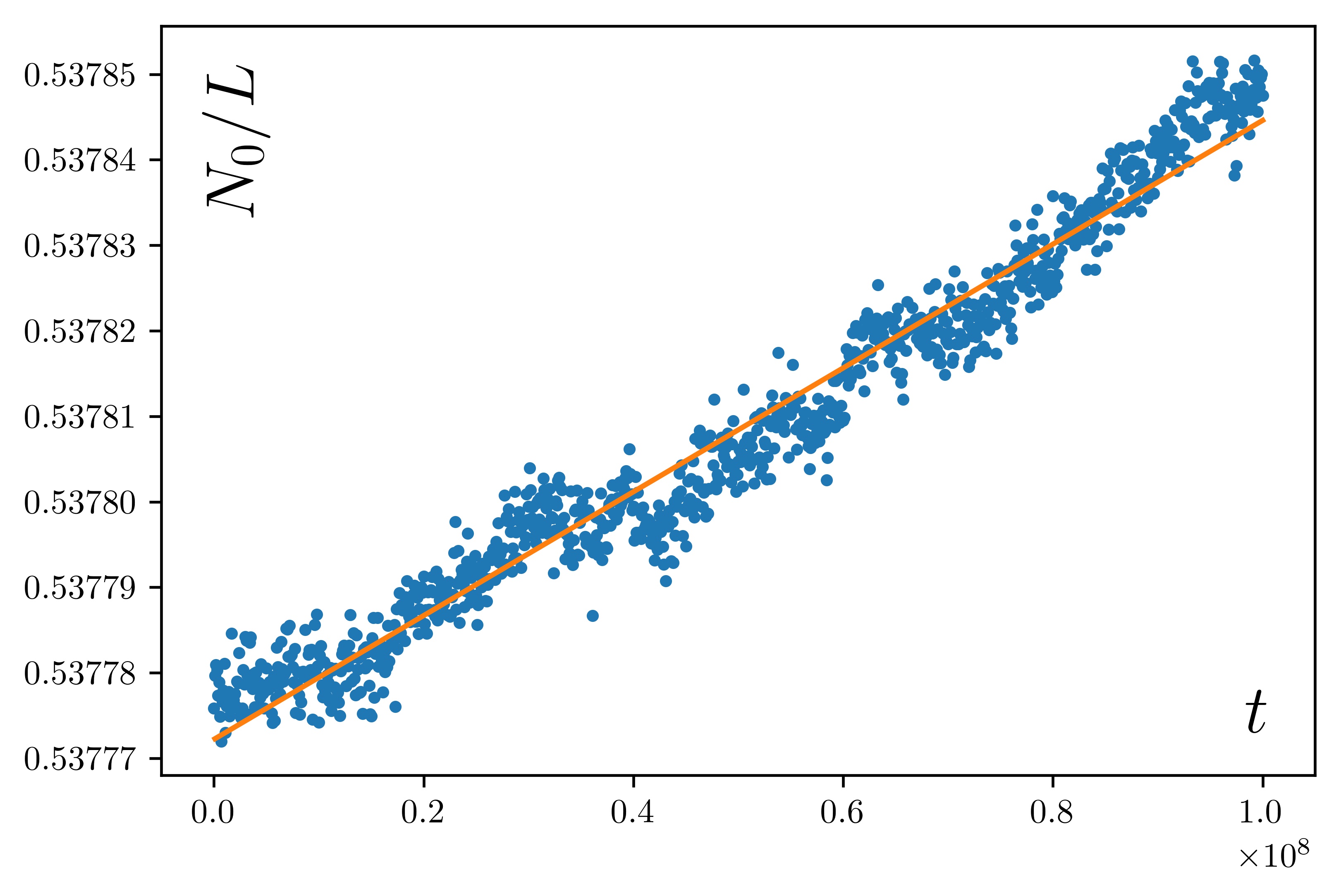
Figure 6: as a function of time for , and (left panel) and (right panel).
The rate is determined by a mean square fit (orange).
Average over more than 250 initial configurations.