Robust Clock Skew and Offset Estimation for IEEE 1588 in the Presence of Unexpected Deterministic Path Delay Asymmetries

Abstract

IEEE 1588, built on the classical two-way message exchange scheme, is a popular clock synchronization protocol for packet-switched networks. Due to the presence of random queuing delays in a packet-switched network, the joint recovery of the clock skew and offset from the timestamps of the exchanged synchronization packets can be treated as a statistical estimation problem. In this paper, we address the problem of clock skew and offset estimation for IEEE 1588 in the presence of possible unknown asymmetries between the deterministic path delays of the forward master-to-slave path and reverse slave-to-master path, which can result from incorrect modeling or cyber-attacks. First, we develop lower bounds on the mean square estimation error for a clock skew and offset estimation scheme for IEEE 1588 assuming the availability of multiple master-slave communication paths and complete knowledge of the probability density functions (pdf) describing the random queuing delays. Approximating the pdf of the random queuing delays by a mixture of Gaussian random variables, we then present a robust iterative clock skew and offset estimation scheme that employs the space alternating generalized expectation-maximization (SAGE) algorithm for learning all the unknown parameters. Numerical results indicate that the developed robust scheme exhibits a mean square estimation error close to the lower bounds.

I Introduction

Clock synchronization is a mechanism to ensure a standard reference time across various devices in a distributed network. This is essential for coordinated activities in a network as time provides the only frame of reference between all devices on the network. Many clock synchronization protocols are available in the literature for synchronizing devices across a packet-switched network. For instance, protocols such as the IEEE 1588 precision time protocol (PTP) [1] and the Network Time Protocol (NTP) [2] are widely used in IP networks, while protocols such as the Timing Protocol for Sensor Networks (TPSN) [3], Lightweight Time Synchronization protocol (LTS) [4] and Reference Broadcast Time synchronization (RBS) protocol [5], are used in wireless sensor networks. In these protocols, the time from a high-cost, high-stability clock (termed master) is distributed to low-cost, low-stability clocks (termed slaves) via an interconnecting network. The clock time at the slave node can be modeled mathematically as a function $c(t)$ of the master node’s clock time $t$, i.e., $c(t)=\phi t+\delta$ [6, 7, 8, 9], where $\phi$ denotes the relative clock skew and $\delta$ denotes the relative clock offset of the slave’s clock time with respect to the master’s clock time. If the clocks at the slave and master node are synchronized, then $c(t)=t$. However, in practice, these clocks are not synchronized, implying a synchronization error $e(t)=|c(t)-t|$ that can grow over time. Time synchronization protocols are utilized to ensure that $e(t)$ remains small.

PTP is a popular clock synchronization protocol used in a number of scenarios, including electrical grid networks [10], cellular base station synchronization in 4G Long Term Evolution (LTE) [11], substation communication networks [12] and industrial control [13]. It is cost-effective and offers accuracy comparable to Global Positioning System (GPS)-based timing. In PTP, as with any clock synchronization protocol built on the two-way message exchange scheme, the slave node exchanges a series of time synchronization packets with the master node and uses the timestamps of these exchanged packets to estimate $\phi$ and $\delta$. The messages traveling between the master and slave nodes can encounter several intermediate switches and routers, accumulating delays at each node. The main factors contributing to the overall delay are: (1) the deterministic (or fixed) propagation and processing delays at the intermediate nodes along the network path between the master and slave nodes and (2) the random queuing delays at each such node. This randomness in the overall network traversal time is referred to as Packet Delay Variation (PDV) [9], and the problem of estimating $\phi$ and $\delta$ in the presence of the PDV is referred to as the “Clock Skew and Offset Estimation” (CSOE) problem. On the other hand, the problem of estimating $\delta$ in the presence of the PDV when $\phi$ is known is referred to as the “Clock Offset Estimation” (COE) problem.

The clock skew and offset can be correctly estimated in PTP (or any time synchronization protocol based on the two-way message exchange scheme such as TPSN and LTS) only if there is a prior known affine relationship between the unknown deterministic path delays in the forward master-to-slave path and the reverse slave-to-master path [14]. However, the presence of an unknown asymmetry between the deterministic path delays can significantly degrade the performance of clock skew and offset estimation schemes [15]. This unknown asymmetry can arise from several sources, including delay attacks [15] and routing asymmetry [16]. In this paper, we look to build on our previous works of [17, 18, 19] to develop joint clock skew and offset estimation schemes that are robust against unknown deterministic path delay asymmetries.

Following [20, 21, 22, 23], we assume the availability of multiple master-slave communication paths in our work. We first develop lower bounds on the best possible performance for invariant clock skew and offset estimation schemes in the presence of possible unknown deterministic path delay asymmetries. Invariant estimators are a reasonable class of estimators in which the estimated parameters scale and shift due to scaling and shifts in the observed timestamps. Also, the commonly employed CSOE schemes in practice are invariant [19]. When developing the performance lower bounds, we assume prior knowledge on whether a master-slave communication path has an unknown asymmetry between the deterministic path delays as well as the complete knowledge of the probability density function (pdf) describing the PDV in the master-slave communication path. The problem of estimating the clock skew and offset in the presence of PDV falls under a variant of the location-scale parameter estimation problems [24], with the unknown clock skew as the scale parameter and the unknown clock offset as the location parameter. Fixing the loss function as the skew-normalized squared error loss, we use invariant decision theory (see Chapter 6 of [24]) to design the optimum approach for combining the information from the various master-slave communication paths to estimate the clock skew and offset. The skew normalized mean square estimation error performance of the developed optimum estimators which assume perfect information (which is usually not available) could be used for comparison against the performance of clock skew and offset estimators that are used in practice. Further, we show the optimum invariant estimators are minimax optimum, i.e., these optimum estimators minimize the maximum skew normalized mean square estimation error over all parameter values.

In specific scenarios, the complete information regarding the pdf of the PDV might not be readily available. To address this issue, we model the pdf of the PDV by a finite mixture of Gaussian distributions. The Gaussian mixture distribution is a prominent model for approximating a pdf as it is a universal approximator in a certain sense [25, 26, 27]. The expectation-maximization (EM) algorithm is a popular iterative approach for obtaining the maximum-likelihood (ML) estimates of the various parameters in problems involving mixture distributions [28, 29]. To obtain closed-form updates for the various parameters, we employ the space alternating generalized Expectation-Maximization (SAGE) algorithm [30], a variant of the EM algorithm, for learning the statistical distribution of the random queuing delays along with the clock skew and offset. The performance of the proposed robust CSOE scheme is evaluated in the LTE backhaul network scenario [11]. In this scenario, PTP is used to synchronize cellular base station clocks using mobile backhaul networks. Typically, the backhaul networks are leased from a commercial Internet Service Provider (ISP), and the network is shared with other commercial and non-commercial users. The background traffic generated by these users results in PDV for the synchronization packets and traffic models for modeling the background traffic are specified in the ITU-T specification G.8261 standard [31]. The class of empirical pdfs corresponding to the PDV according to the ITU-T specification G.8261 [31] was derived in [9]. In our work, we use the empirical pdfs obtained in [9] to evaluate the developed lower bounds as well as the performance of the proposed robust CSOE scheme. Numerical results indicate that the proposed scheme exhibits a skew normalized mean square estimation error close to the performance lower bounds.

I-A Related work

In this paper, we have developed a algorithm for jointly estimating the clock skew and offset for PTP (or any clock synchronization protocol based on the two-way message exchange) that is robust against unknown deterministic path delay asymmetries. To the best of our knowledge, there is no such algorithm available in the literature that addresses the problem of jointly estimating clock skew and offset in the presence of unknown deterministic path delay asymmetries. In this section, we present several approaches available in the literature for synchronizing devices in a network, none of which address the problem of jointly estimating clock skew and offset in the presence of unknown deterministic path delay asymmetries. Data Center Time Protocol (DTP) is a clock synchronization protocol that does not use packets, but rather uses the physical layer of network devices to implement a decentralized clock synchronization protocol [32]. DTP, however, requires additional hardware, necessitating a fully “DTP-enabled network” for its deployment [33]. HUYGENS [33] is a software-based clock synchronization system that incorporates Support Vector Machines and was proposed as an alternative to DTP for synchronizing devices in a data center. In [34], the authors proposed R-Sync, a time synchronization scheme for the industrial Internet of things (IIoT) as an alternative to existing time synchronization algorithms such as TPSN. Although these protocols offer interesting alternatives to PTP, in our work, we primarily look at improving the performance of PTP (or any clock synchronization protocol based on the two-way message exchange) in the presence of PDV and possible unknown asymmetries between the deterministic path delays in the forward and reverse paths.

We now briefly describe some of the popular algorithms available in the literature that have been developed for clock synchronization protocols built on the two-way message exchange scheme and assume a known relationship between the deterministic path delays of the forward and reverse paths [6, 7, 35, 36, 37, 9, 38]. The ML estimate and the corresponding Cramer-Rao bound (CRB) for the CSOE problem under the Gaussian PDV pdf delay model were derived in [6]. Under the exponential PDV pdf delay model, the ML estimate of the clock skew and offset was derived in [7, 36] and the minimum variance unbiased estimate (MVUE) for the COE problem was derived in [35]. CSOE schemes for PTP that incorporate linear programming were proposed in [37]. For an arbitrary pdf-delay model of PDV, the optimum invariant estimator for the COE problem and CSOE problem was derived in [9] and [19], respectively. Further, in [38], the authors developed a sub-optimal clock offset estimation scheme based on the linear combination of order statistics that exhibits performance close to the performance of the optimum clock offset estimator developed in [9].

We now describe some of the algorithms available in the literature for clock synchronization protocols based on the two-way message exchange scheme which do not assume a prior known relationship between the deterministic path delays of the forward and reverse paths [39, 20, 21, 22, 17, 18]. In [39], the authors proposed a COE scheme that uses the median of the observed timing offsets from different master nodes to estimate the clock offset. The proposed scheme is robust against unknown deterministic path delay asymmetries, however, there is a loss in performance due to the significant amount of information being discarded. In [20], the authors proposed the idea of using a group of masters rather than a single master for synchronizing the slave node. The proposed COE scheme works in the presence of a master node failure or a master-slave communication path having unknown deterministic path delay asymmetries. However, it requires prior information regarding the number of the master-slave communication paths that have unknown deterministic path delay asymmetries. This information might not be readily available in many scenarios. Mizrahi [21, 22] proposed the use of multiple master-slave communication paths to improve the accuracy of clock offset estimation schemes assuming clock skew is known and also to help protect against delay attacks (a particular case of unknown deterministic path delay asymmetries). Previously, assuming complete knowledge of the clock skew, we developed performance lower bounds along with robust clock offset estimation schemes for PTP that can handle unknown deterministic path delay asymmetries [17, 18]. However, to the best of our knowledge, there is no algorithm available in the literature for the joint estimation of the clock skew and offset that can handle unknown deterministic path delay asymmetries. None of the algorithms presented in [6, 7, 40, 35, 8, 36, 37, 9, 38, 39, 20, 21, 22, 17, 18] address the problem of jointly estimating the clock skew and offset for PTP in the presence possible unknown deterministic path delay asymmetries.

I-B Notations used

We use bold upper case, bold lower case, and italic lettering to denote matrices, column vectors and scalars respectively. The notations $(.)^{T}$ and $\otimes$ denote the transpose and Kronecker product, respectively. $\bm{I}_{N}$ stands for a $N$-dimensional identity matrix, $\mathbbm{1}_{N}$ denotes a column vector of length $N$ with all the elements equal to $1$ and $\bm{0}_{N}$ denotes a column vector of length $N$ with all the elements equal to $0$. Further, $\mathbb{R}$ denotes the set of real numbers, $\mathbb{R}^{+}$ denotes the set of positive real numbers, $\mathbb{R}^{+}_{0}$ denotes the set of non-negative real numbers and $\mathcal{I}_{A}(x)$ denotes the indicator function having the value $1$ when $x\in A$ and $0$ when $x\notin A$.

II Signal Model and Problem Statement

In this section, we briefly describe the two-way message exchange scheme used in PTP and present the considered problem statement along with the assumptions. We assume the availability of $N$ master-slave communication paths and perfect synchronization between the clocks of the $N$ masters. Recall that the relative clock skew and offset of the slave node with respect to a master node are denoted by $\phi\in\mathbb{R}^{+}$ and $\delta\in\mathbb{R}$, respectively. Assume a total of $P$ rounds of two-way message exchanges at each master-slave communication path. The following sequence of messages are exchanged over the $i^{\mbox{th}}$ master-slave communication path during the $j^{\mbox{th}}$ round of message exchanges: The master node initiates the exchange by sending a sync packet to the slave at time $t_{1ij}$. The value of $t_{1ij}$ is later communicated to the slave via a follow_up message. The slave node records the time of reception of the sync message as $t_{2ij}$. The slave node sends a delay_req message to the master node recording the time of transmission as $t_{3ij}$. The master records the time of arrival of the delay_req packet at time $t_{4ij}$ and this value is later communicated to the slave using a delay_resp packet. The relationship between the received timestamps are given by [6, 7, 35, 8]

$$t_{2ij}=(t_{1ij}+d_{i}^{ms}+w_{1ij})\phi+\delta t_{3ij}=(t_{4ij}-d_{i}^{sm}-w_{2ij})\phi+\delta,$$ ; (1)

for $i=1,2,\cdots,N$ and $j=1,2,\cdots,P$. In (1), $d_{i}^{ms}$ and $d_{i}^{sm}$ denote the unknown deterministic path delays in the forward and reverse path, respectively, at the $i^{\mbox{th}}$ master-slave communication path. The variables $w_{1ij}$ and $w_{2ij}$ denote the random queuing delays in the forward and reverse path, respectively, during the $j^{\mbox{th}}$ round of message exchanges for the $i^{\mbox{th}}$ master-slave communication path. The pdf of $\{w_{kij}\}^{P}_{j=1}$ is denoted by $f_{ki}(.)$ for $k=1,2$ and $i=1,2,\cdots,N$.

Freris et al. [14] provided the necessary conditions for obtaining a unique solution to the clock skew and offset for protocols based on a two-way message exchange scheme for a single forward-reverse path pair of timestamps. We need to know either one of the deterministic path delays (either the deterministic delay of the forward path or the deterministic delay of the reverse path), or have a prior known affine relationship between the unknown deterministic path delays (see Theorem 4 in [14]). Synchronization protocols including PTP [1], NTP [2], TPSN [3] used in real networks generally assume that the deterministic path delays in the forward and reverse paths are equal. In this paper, we classify a master-slave communication path as being symmetric or asymmetric depending on the relationship between the deterministic path delays. A symmetric master-slave communication path denotes a master-slave communication path in which the deterministic path delays in the forward and reverse paths are equal, i.e., $d^{ms}_{i}=d^{sm}_{i}=d_{i}$, where $d_{i}$ denotes the unknown deterministic path delay over the $i^{\mbox{th}}$ master-slave communication path. Similarly, an asymmetric master-slave communication path denotes a master-slave communication path having an unknown asymmetry between the deterministic path delays in the forward and reverse paths, i.e., $d^{ms}_{i}=(d_{i}+\tau_{i})$ and $d^{sm}_{i}=d_{i}$. The parameter $\tau_{i}$ denotes the constant (for all $j$) unexpected asymmetry between the deterministic path delays.

Define $\bm{w}_{ki}=[w_{ki1},w_{ki2},\cdots,w_{kiP}]^{T}$ for $k=1,2$, $i=1,2,\cdots,N$ and $\bm{t}_{ki}=[t_{ki1},t_{ki2},\cdots,$ $t_{kiP}]^{T}$ for $k=1,2,3,4$, $i=1,2,\cdots,N$. We now introduce a new binary state vector variable $\bm{\eta}=[\eta_{1},\eta_{2},\cdots,\eta_{N}]$, which indicates whether a master-slave communication path is symmetric or asymmetric. The $i^{\mbox{th}}$ element of $\bm{\eta}$ is $1$ when the $i^{\mbox{th}}$ master-slave communication path is asymmetric, else it has a value of $0$. If $\eta_{i}=0$, the received timestamps from the $i^{\mbox{th}}$ master-slave communication path can be arranged in vector form as

$$\bm{t}_{2i}=(\bm{t}_{1i}+d_{i}\mathds{1}_{P}+\bm{w}_{1i})\phi+\delta\mathds{1}_{P} \bm{t}_{3i}=(\bm{t}_{4i}-d_{i}\mathds{1}_{P}-\bm{w}_{2i})\phi+\delta\mathds{1}_{P}.$$ ; (2)

Similarly, when $\eta_{i}=1$, the received timestamps from the $i^{\mbox{th}}$ master-slave communication path can be arranged in vector form as

$$\bm{t}_{2i}=(\bm{t}_{1i}+(d_{i}+\tau_{i})\mathds{1}_{P}+\bm{w}_{1i})\phi+\delta\mathds{1}_{P} \bm{t}_{3i}=(\bm{t}_{4i}-d_{i}\mathds{1}_{P}-\bm{w}_{2i})\phi+\delta\mathds{1}_{P}.$$ ; (3)

The complete set of received timestamps is denoted by $\bm{t}=[\bm{t}_{11},\bm{t}_{12},\cdots,\bm{t}_{1N},\bm{t}_{21},\bm{t}_{22},\cdots$, $\bm{t}_{2N},\bm{t}_{31},\bm{t}_{32},\cdots,\allowbreak\bm{t}_{3N},\bm{t}_{41},\bm{t}_{42},\cdots,\bm{t}_{4N}]$. In our work, we seek estimators of $\delta$ and $\phi$ from the received timestamps $\bm{t}$, when $\bm{\eta}$ is unknown. We now state the assumptions made in our work.

Assumption 1: Following [20, 21, 22, 23], we assume the availability of $N$ master-slave communication paths and further assume that fewer than half of the $N$ master-slave communication paths are asymmetric, i.e., $||\bm{\eta}||_{1}<N/2$. The latter assumption of $||\bm{\eta}||_{1}<N/2$ is sufficient to identify the symmetric paths after clustering. Having some protected paths would be an alternative.

Assumption 2: All the queuing delays are strictly positive random variables and have finite support. Following [6, 7, 35, 36, 8, 37, 9, 38, 17, 19], we assume that the random queuing delays $\{w_{kij}\}^{P}_{j=1}$ are independent and identically distributed in our work. The pdf of the random variables are denoted by $f_{ki}(.)$ for $i=1,2,\cdots,N$, $k=1,2$. Usually, the two-way timing message exchanges are sufficiently spaced apart in time to ensure that the random queuing delays are independent. Further the background traffic patterns in networks remain constant over several minutes. Hence, the assumption that all queuing delays in a particular master-slave communication path share a common pdf is fairly realistic.

Assumption 3: Following [6, 7, 35, 8], we assume the unknown deterministic path delays $\{d_{i}\}_{i=1}^{N}$, unknown biases $\{\tau_{i}\}_{i=1}^{N}$, clock skew $\phi$ and the clock offset $\delta$ are constant over $P$ two-way message exchanges for each master-slave communication path.

Assumption 4: As very small $\tau_{i}$ will have little impact, we officially define a master-slave communication path as having an unknown asymmetry ($\eta_{i}=1$) when $|\tau_{i}|\geq d_{\tau}$, where $d_{\tau}$ can be chosen such that $|\tau_{i}|<d_{\tau}$ causes little impact.

III Performance Lower Bounds For a Robust Clock Skew and Offset Estimation Scheme

In this section, we develop useful performance lower bounds that help in evaluating the performance of the proposed clock skew and offset estimation schemes that are robust to unknown path asymmetries. We assume $\bm{\eta}$ is known and further assume complete knowledge of $f_{ki}(.)$ for $i=1,2,\cdots,N$ and $k=1,2$. We use invariant decision theory (see chapter $6$ of [24]) to develop the optimum approach for fusing information from the $N$ master-slave communication paths. For ease of notation, we assume the first $K(<N/2)$ master-slave communication paths are asymmetric and the remaining $(N-K)$ master-slave communication paths are symmetric. Under these assumptions with (2) and (3), we obtain

$$\bm{y}_{i} = (\bm{h}d_{i}+\bm{g}\tau_{i}+\bm{v}_{i})\phi+\delta\mathds{1}_{2P},$$ (4)

for $i=1,2,\cdots,K$ and

$$\bm{y}_{i} = (\bm{h}d_{i}+\bm{v}_{i})\phi+\delta\mathds{1}_{2P},$$ (5)

for $i=K+1,\cdots,N$. In (4) and (5), $\bm{y}_{i}=[\bm{t}_{2i}^{T},\bm{t}_{3i}^{T}]^{T}$, $\bm{h}=[\mathds{1}_{P}^{T},-\mathds{1}_{P}^{T}]^{T}$, $\bm{g}=[\mathds{1}_{P}^{T},\bm{0}_{P}^{T}]^{T}$ and $\bm{v}_{i}=[\bm{v}_{1i}^{T},\bm{v}_{2i}^{T}]^{T}$ with $\bm{v}_{1i}=(\bm{t}_{1i}+\bm{w}_{1i})$ and $\bm{v}_{2i}=(\bm{t}_{4i}-\bm{w}_{2i})$. The complete set of observations from the $N$ master-slave communication paths can be represented in vector form as

$$\bm{y} = (\bm{H}\bm{\gamma}+\bm{v})\phi+\delta\mathds{1}_{2NP},$$ (6)

where $\bm{y}=[\bm{y}_{1}^{T},\bm{y}_{2}^{T},\cdots,\bm{y}_{N}^{T}]$, $\bm{v}=[\bm{v}_{1}^{T},\bm{v}_{2}^{T},\cdots,\bm{v}_{N}^{T}]$ and $\bm{\gamma}=[\bm{d},\bm{\tau}]$ with $\bm{d}=[d_{1},d_{2},\cdots,d_{N}]$ and $\bm{\tau}=[\tau_{1},\tau_{2},\cdots,\tau_{K}]$ and $\bm{H}=\begin{bmatrix}\bm{h}\otimes\bm{I}_{N},\bm{g}\otimes\bm{I}_{K}\end{bmatrix}$. Let $\bm{\theta}=[\phi,\delta,d_{1},d_{2},\cdots,d_{N},\tau_{1},\cdots,\tau_{K}]$ denote the vector of unknown parameters. The parameter space of $\bm{\theta}$, denoted by $\bm{\Theta}$, is given by $\bm{\Theta}=\{(\phi,\delta,\bm{d},\bm{\tau}):\phi\in\mathbb{R}^{+},{\delta}\in\mathbb{R},\bm{d}\in\mathbb{R}^{N},\bm{\tau}\in\mathbb{R}^{K}\}$. From (6), the conditional pdf of $\bm{y}$ is given by

$$f(\bm{y}|\bm{\theta})= \frac{1}{\phi^{2NP}}f_{\bm{v}}\left(\frac{\bm{y}-\delta\mathds{1}_{2NP}}{\phi}-\bm{H}\bm{\gamma}\right),$$ (7)

$$= \frac{1}{\phi^{2NP}}\prod_{i=1}^{K}f_{\bm{v}_{i}}\left(\frac{\bm{y}_{i}-\delta\mathds{1}_{2P}}{\phi}-d_{i}\bm{h}-\tau_{i}\bm{g}\right)\prod_{i=K+1}^{N}f_{\bm{v}_{i}}\left(\frac{\bm{y}_{i}-\delta\mathds{1}_{2P}}{\phi}-d_{i}\bm{h}\right),$$ (8)

where $f_{\bm{v}_{i}}(\bm{v}_{i})=\prod_{j=1}^{P}f_{1i}\left({v}_{1ij}-{t}_{1ij}\right)f_{2i}\left({t}_{4ij}-{v}_{2ij}\right)$ for $i=1,2,\cdots,N$. Let $\mathcal{F}_{M}$ denote the class of all pdfs $f(\bm{y}|\bm{\theta})$ for $\bm{\theta}\in\bm{\Theta}$. The class of such pdfs is invariant under the group of transformations $\mathcal{G}_{M}$ on the observations $\bm{y}$, on $\mathbb{R}^{2NM}$, defined as

$$\mathcal{G}_{M} =\{g_{a,\bm{b},c}(\bm{y}):g_{a,\bm{b},c}(\bm{y})=(\bm{y}+\bm{H}\bm{b})a+c\mathds{1}_{2NP},\forall(a,\bm{b},c)\in\mathbb{R}^{+}\times\mathbb{R}^{N+K}\times\mathbb{R}\},$$ (9)

where $\bm{y}\in\mathbb{R}^{2NM}$, since $\bm{y}_{g}=g_{a,\bm{b},{c}}(\bm{y})$ has a pdf given by $\frac{1}{(a\phi)^{2NM}}$ $f_{\bm{v}}\left(\frac{\bm{y}_{g}-((a{\delta}+{c})\mathds{1}_{2NP})}{a\phi}\allowbreak-\bm{H}\left(\bm{\gamma}+\frac{\bm{b}}{\phi}\right)\right)$. The corresponding group of induced transformations on $\bm{\Theta}$, denoted by $\bar{\mathcal{G}}_{M}$, is given by

$$\bar{\mathcal{G}}_{M} =\{\bar{g}_{a,\bm{b},{c}}((\phi,\bm{\gamma},{\delta})):\bar{g}_{a,\bm{b},{c}}((\phi,\bm{\gamma},{\delta}))=(a\phi,(\bm{\gamma}+\bm{b}/\phi),(a{\delta}+{c})),\forall(a,\bm{b},c)\in\mathbb{R}^{+}\times\mathbb{R}^{N+K}\times\mathbb{R}\},$$ (10)

where $\phi\in\mathbb{R}^{+},\bm{\gamma}\in\mathbb{R}^{N+K}$ and ${\delta}\in\mathbb{R}$.

Let $\hat{\delta}_{I}$ and $\hat{\phi}_{I}$ denote estimators of $\delta$ and $\phi$, respectively and let $\hat{\delta}_{I}(\bm{y})$ and $\hat{\phi}_{I}(\bm{y})$ denote the estimates obtained from the received data $\bm{y}$ characterized by the pdf $f(\bm{y}|\bm{\theta})=\frac{1}{\phi^{2NP}}\allowbreak f_{\bm{v}}\left(\frac{\bm{y}-({\delta}\mathds{1}_{2NP})}{\phi}-\bm{H}\bm{\gamma}\right)$. From (10), the estimators $\hat{\phi}_{I}(\bm{y})$ and $\hat{\delta}_{I}(\bm{y})$ are invariant under $\mathcal{G}_{M}$ from (9), if for all $(a,\bm{b},{c})\in\mathbb{R}^{+}\times\mathbb{R}^{N+K}\times\mathbb{R}$,

$$\hat{\delta}_{I}(g_{a,\bm{b},c}(\bm{y}))=\hat{\delta}_{I}(a(\bm{y}+\bm{Hb})+{c}\mathds{1}_{2NP}) =a\hat{\delta}_{I}(\bm{y})+c,$$ (11)

$$\hat{\phi}_{I}(g_{a,\bm{b},{c}}(\bm{y}))=\hat{\phi}_{I}(a(\bm{y}+\bm{Hb})+{c}\mathds{1}_{2NP}) =a\hat{\phi}_{I}(\bm{y}).$$ (12)

In this paper, we consider the skew-normalized squared error loss functions for $\delta$ and $\phi$ defined by $\frac{(\hat{\delta}_{I}(\bm{y})-\delta)^{2}}{\phi^{2}}$ and $\frac{(\hat{\phi}_{I}(\bm{y})-\phi)^{2}}{\phi^{2}}$, respectively. The corresponding conditional risk for $\hat{\delta}_{I}$ and $\hat{\phi}_{I}$ under the skew normalized square error loss functions are the skew-normalized mean square estimation errors, defined by

$$\mathcal{R}(\hat{\delta}_{I},\bm{\theta})=\frac{1}{\phi^{2}}\int_{\mathbb{R}^{2NM}}(\hat{\delta}_{I}(\bm{y})-\delta)^{2}f(\bm{y}|\bm{\theta})d\bm{y} \mathcal{R}(\hat{\phi}_{I},\bm{\theta})=\frac{1}{\phi^{2}}\int_{\mathbb{R}^{2NM}}(\hat{\phi}_{I}(\bm{y})-\phi)^{2}f(\bm{y}|\bm{\theta})d\bm{y},$$ ; (13)

respectively. The skew-normalized loss functions for $\delta$ and $\phi$ are invariant under $\mathcal{G}_{M}$ from (9), since

$$\frac{(\hat{\delta}_{I}(\bm{y})-\delta)^{2}}{\phi^{2}}=\frac{\left(\hat{\delta}_{I}(g_{a,\bm{b},{c}}(\bm{y}))-(a\delta+c)\right)^{2}}{a^{2}\phi^{2}}\mbox{ and }\frac{(\hat{\phi}_{I}(\bm{y})-\phi)^{2}}{\phi^{2}}=\frac{\left(\hat{\phi}_{I}(g_{a,\bm{b},{c}}(\bm{y}))-a\phi\right)^{2}}{a^{2}\phi^{2}},$$ (14)

for all $g_{a,\bm{b},{c}}\in\mathcal{G}_{M}$. We now present the optimum invariant (or minimum conditional risk) estimators of $\delta$ and $\phi$.

Proposition 1.

(Genie Bound) Assuming knowledge of the paths having an unknown asymmetry and complete knowledge of $f_{1i}(.)$ and $f_{2i}(.)$ for $i=1,2,\cdots,N$, the optimum invariant estimators for $\delta$ and $\phi$, denoted by $\hat{\delta}_{opt}$ and $\hat{\phi}_{opt}$, respectively, are given by

$$\hat{\delta}_{opt}(\bm{y}) =\frac{\int_{\mathbb{R}^{+}}\int_{\mathbb{R}^{N+K+1}}\frac{\delta\Gamma_{1}(\phi,\delta,\bm{d},\bm{\tau},\bm{y})\Gamma_{0}(\phi,\delta,\bm{d},\bm{y})}{\phi^{2NP-N-K+3}}d\bm{\tau}d(\bm{d})d\delta d\phi}{\int_{\mathbb{R}^{+}}\int_{\mathbb{R}^{N+K+1}}\frac{\Gamma_{1}(\phi,\delta,\bm{d},\bm{\tau},\bm{y})\Gamma_{0}(\phi,\delta,\bm{d},\bm{y})}{\phi^{2NP-N-K+3}}d\bm{\tau}d(\bm{d})d\delta d\phi},$$ (15)

and

$$\hat{\phi}_{opt}(\bm{y}) =\frac{\int_{\mathbb{R}^{+}}\int_{\mathbb{R}^{N+K+1}}\frac{\Gamma_{1}(\phi,\delta,\bm{d},\bm{\tau},\bm{y})\Gamma_{0}(\phi,\delta,\bm{d},\bm{y})}{\phi^{2NP-N-K+2}}d\bm{\tau}d(\bm{d})d\delta d\phi}{\int_{\mathbb{R}^{+}}\int_{\mathbb{R}^{N+K+1}}\frac{\Gamma_{1}(\phi,\delta,\bm{d},\bm{\tau},\bm{y})\Gamma_{0}(\phi,\delta,\bm{d},\bm{y})}{\phi^{2NP-N-K+3}}d\bm{\tau}d(\bm{d})d\delta d\phi},$$ (16)

respectively, where we have $\Gamma_{1}(\phi,\delta,\bm{d},\bm{\tau},\bm{y})=\prod_{i=1}^{K}f_{\bm{v}_{i}}\left(\frac{\bm{y}_{i}-\delta\bm{1}_{2M}}{\phi}-d_{i}\bm{h}-\tau_{i}\bm{g}\right)$ and $\Gamma_{0}(\phi,\delta,\bm{d},\bm{y})=\allowbreak\prod_{i=K+1}^{N}\allowbreak f_{\bm{v}_{i}}\left(\frac{\bm{y}_{i}-\delta\bm{1}_{2M}}{\phi}-d_{i}\bm{h}\right)$. Following a proof similar to that given in [19], we can show the estimators $\hat{\delta}_{opt}$ and $\hat{\phi}_{opt}$ are minimax optimum, i.e., they minimize the maximum of the skew-normalized mean square estimation error (NMSE) over all parameter values. As these optimum estimators achieve the smallest NMSE among the class of invariant estimators and are minimax optimum, the performance of these estimators give us useful fundamental lower bounds on the skew-normalized mean square estimation error for a clock skew and offset estimation scheme. We refer to the clock skew and offset estimators presented in (15) and (16) as genie optimum estimators.

In certain scenarios where we have analytical expressions for $f_{1i}(.)$ and $f_{2i}(.)$ for $i=1,2,\cdots,N$, it might be possible to further simplify the integrals in (15) and (16). However, for the general case of arbitrary queuing delay pdfs, these integrals are computed by approximating them with Riemann summations. The width of the Riemann summation bins is set to small values to ensure that the additional error introduced due to the Riemann sum approximation is insignificant relative to the estimation error.

Remark.

Proposition 1 provides us with mathematical expressions for the optimum clock skew and offset estimators for IEEE 1588 under the assumption that we have complete knowledge of $f_{1i}(.)$ and $f_{2i}(.)$ for $i=1,2,\cdots,N$ and prior knowledge of the master-slave communication paths having unknown deterministic path asymmetries. The skew normalized mean square estimation error (NMSE) performance of the optimum estimators described in Proposition 1 cannot be achieved unless we have information that is usually not available (prior information regarding the master-slave communication paths having unknown deterministic path delay asymmetries). Hence, the NMSE performance of the optimum clock skew and offset estimator described in Proposition 1 can be viewed as a performance lower bound. The NMSE performance of the optimum clock skew and offset estimator described in Proposition 1 can be viewed as a performance lower bound as it gives us a lower bound on the NMSE for invariant clock skew and offset estimation schemes in the presence of possible unknown deterministic path delay asymmetries.

IV Robust Clock Skew and Offset Estimation Scheme

In this section, we present our robust scheme for jointly estimating the clock skew and offset in the presence of master-slave communication paths with possible unknown asymmetries. When developing the performance bounds in Proposition 1, we had assumed prior information regarding the paths having an unknown asymmetry as well as the complete knowledge of the distribution of the queuing delays. However in practice, we generally do not have information regarding the asymmetric master-slave communication paths. Hence, we attempt to identify these paths when developing a robust clock skew and offset scheme. Further in some scenarios, we might not have the complete information regarding the pdf of the random queuing delays, $f_{1i}(.)$ and $f_{2i}(.)$ for $i=1,2,\cdots,N$. In this paper, we use the popular Gaussian mixture model (GMM) [26, 27] for approximating the pdf of the random queuing delays as

$$f_{1i}(w)=\sum_{k=1}^{M_{i}}\alpha_{ik}\mathcal{P}_{\mu_{1ik},\sigma_{1ik}}\left(w\right) f_{2i}(w)=\sum_{l=1}^{L_{i}}\beta_{il}\mathcal{P}_{\mu_{2il},\sigma_{2il}}\left(w\right),$$ ; (17)

for $i=1,2,\cdots,N$. In (17), $\{\alpha_{ik}\}_{k=1}^{M_{i}}$ and $\{\beta_{il}\}_{l=1}^{L_{i}}$ denote the unknown mixing coefficients in the forward and reverse path at the $i^{\mbox{th}}$ master-slave communication path with $M_{i}$ and $L_{i}$ denoting the number of assumed mixture components in the forward and reverse path, respectively. Also, we have $\alpha_{ik}\in[0,1]$ and $\beta_{il}\in[0,1]$ with the constraints $\sum_{k=1}^{M_{i}}\alpha_{ik}=1$ and $\sum_{l=1}^{L_{i}}\beta_{il}=1$. Further, $\mathcal{P}_{\mu,\sigma}(.)$ denotes a normal distribution with mean $\mu$ and standard deviation $\sigma$. The variables $\{\mu_{1ik},\sigma_{1ik}\}$ denote the mean and standard deviation of the $k^{\mbox{th}}$ component in the mixture models in the $i^{\mbox{th}}$ forward path and the variables $\{\mu_{2il},\sigma_{2il}\}$ denote the mean and standard deviation of the $l^{\mbox{th}}$ component in the mixture models in the $i^{\mbox{th}}$ reverse path. A set of samples $\tilde{\bm{w}}_{k}=[\tilde{\bm{w}}_{k1},\tilde{\bm{w}}_{k2},\cdots,\tilde{\bm{w}}_{kN}]$ for $k=1,2$, where $\tilde{\bm{w}}_{ki}=[\tilde{{w}}_{ki1},\tilde{{w}}_{ki2},\cdots,\tilde{{w}}_{kiP_{t}}]$ for $i=1,2,\cdots,N$ are obtained from the previous block of $P_{t}$ two-way message exchanges which we call the previous window as we describe next. The full impact of using these samples is characterized in Section V, where it is shown that in the cases studied, they provide positive impact. Let the received timestamps corresponding to the previous block be denoted by $\tilde{\bm{t}}_{ki}=[\tilde{t}_{ki1},\tilde{t}_{ki2},\cdots,$ $\tilde{t}_{kiP_{t}}]$ for $k=1,2,3,4$ and $i=1,2,\cdots,N$ and the previous estimates of the $\delta$, $\phi$, $d_{i}^{ms}$ and $d_{i}^{sm}$ for $i=1,2,\cdots,N$ be denoted by $\tilde{\delta}^{old}$, $\tilde{\phi}^{old}$, $\tilde{d}_{i}^{ms}$ and $\tilde{d}_{i}^{sm}$ for $i=1,2,\cdots,N$, respectively. From (1), we then obtain $\tilde{\bm{w}}_{k}$ for $k=1,2$ as

$$\tilde{\bm{w}}_{1i}=\frac{\tilde{\bm{t}}_{2i}-\tilde{\delta}^{old}\mathds{1}_{P_{t}}}{\tilde{\phi}^{old}}-\tilde{\bm{t}}_{1i}-\tilde{d}_{i}^{ms}\mathds{1}_{P_{t}}; \qquad\tilde{\bm{w}}_{2i}=\frac{\tilde{\delta}^{old}\mathds{1}_{P_{t}}-\tilde{\bm{t}}_{3i}}{\tilde{\phi}^{old}}+\tilde{\bm{t}}_{4i}-\tilde{d}_{i}^{sm}\mathds{1}_{P_{t}}$$ (18)

for $i=1,2,\cdots,N.$

Let $\bm{\Omega}$ denote the vector of unknown parameters defined as $\bm{\Omega}=[\bm{\Psi},\bm{\eta},\bm{\alpha}_{1},\cdots,\bm{\alpha}_{N},\bm{\beta}_{1},\cdots,\bm{\beta}_{N},\bm{\mu}_{11},\cdots$ $\bm{\mu}_{1N},\bm{\sigma}_{11},\cdots,\bm{\sigma}_{1N},\bm{\mu}_{21},\cdots,\bm{\mu}_{2N},\bm{\sigma}_{21},\cdots,\bm{\sigma}_{2N}]$ where we have $\bm{\Psi}=[\phi,\delta,d_{1},\cdots,d_{N},\tau_{1},\cdots,\tau_{N}]$, $\bm{\eta}=[\eta_{1},\eta_{2},\cdots,\eta_{N}]$, $\bm{\alpha}_{i}=[\alpha_{i1},\cdots,\alpha_{iM_{i}}]$ for $i=1,2,\cdots,N$, $\bm{\beta}_{i}=[\beta_{i1},\cdots,\beta_{iL_{i}}]$ for $i=1,2,\cdots,N$, $\bm{\mu}_{1i}=[\mu_{11},\cdots,\mu_{1M_{i}}]$ for $i=1,2,\cdots,N$, $\bm{\mu}_{2i}=[\mu_{21},\cdots,\mu_{2L_{i}}]$ for $i=1,2,\cdots,N$, $\bm{\sigma}_{1i}=[\sigma_{1i1},\cdots,\sigma_{1iM_{i}}]$ for $i=1,2,\cdots,N$ and $\bm{\sigma}_{2i}=[\sigma_{2i1},\cdots,\sigma_{2iL_{i}}]$ for $i=1,\cdots,N$. Given $\bm{\Omega}$, the log-likelihood function of the observed data $\bm{t}$, $\tilde{\bm{w}}_{1}$ and $\tilde{\bm{w}}_{2}$, denoted by $\mathcal{L}(\bm{\Omega}|\bm{t},\tilde{\bm{w}}_{1},\tilde{\bm{w}}_{2})$, is defined as

$$\sum_{i=1}^{N}\sum_{j=1}^{P}\Bigg{[}\ln\left(\eta_{i}\Bigg{(}\sum_{k=1}^{M_{i}}\alpha_{ik}\mathcal{P}_{\mu_{1ik},\sigma_{1ik}}\left(\frac{t_{2ij}-\delta}{\phi}-d_{i}-\tau_{i}\right.\right.\left.-t_{1ij}\right)\Bigg{)}\left.\Bigg{(}\sum_{l=1}^{L_{i}}\beta_{il}\mathcal{P}_{\mu_{2il},\sigma_{2il}}\left(t_{4ij}-d_{i}+\frac{\delta-t_{3ij}}{\phi}\right)\right)\Bigg{)}$$

$$+(1-\eta_{i})\left(\sum_{k=1}^{M_{i}}\alpha_{ik}\mathcal{P}_{\mu_{1ik},\sigma_{1ik}}\left(\frac{t_{2ij}-\delta}{\phi}-d_{i}-t_{1ij}\right)\right.\Bigg{)}\left.\Bigg{(}\sum_{l=1}^{L_{i}}\beta_{il}\mathcal{P}_{\mu_{2il},\sigma_{2il}}\left(t_{4ij}-d_{i}+\frac{\delta-t_{3ij}}{\phi}\right)\right)\Bigg{)}\Bigg{]}$$

$$+\sum_{i=1}^{N}\sum_{j=1}^{P_{t}}\ln\left(\sum_{k=1}^{M_{i}}\alpha_{ik}\mathcal{P}_{\mu_{1ik},\sigma_{1ik}}(\tilde{w}_{1ij})\right)+\sum_{i=1}^{N}\sum_{j=1}^{P_{t}}\ln\left(\sum_{l=1}^{L_{i}}\beta_{il}\mathcal{P}_{\mu_{2il},\sigma_{2il}}(\tilde{w}_{2ij})\right)-2NM\ln\phi.$$ (19)

The maximum likelihood method is widely used and has many attractive features including consistency and asymptotic unbiasedness. Under assumptions $1-3$, the maximum likelihood estimate (MLE) of $\bm{\Omega}$, denoted by $\hat{\bm{\Omega}}_{mle}$, is obtained by solving the following constrained optimization problem.

$$\hat{\bm{\Omega}}_{mle} =\operatorname*{arg\,max}_{\bm{\Omega}}\mathcal{L}(\bm{\Omega}|\bm{t},\tilde{\bm{w}}_{1},\tilde{\bm{w}}_{2})$$ (20)

$$\mbox{ such that }\eta_{i} \in\{0,1\}\mbox{ for }i=1,2,\cdots,N,$$ (20a)

$$\alpha_{ik} \in[0,1]\mbox{ for }i=1,2,\cdots,N,k=1,2,\cdots,M\mbox{, }\sum_{k=1}^{M_{i}}\alpha_{ik}=1,$$ (20b)

$$\beta_{il} \in[0,1]\mbox{ for }i=1,2,\cdots,N\mbox{, }l=1,2,\cdots,M\mbox{, }\sum_{l=1}^{L_{i}}\beta_{il}=1,$$ (20c)

$$|\tau_{i}| \geq d_{\tau}\mbox{ when }\eta_{i}=1,$$ (20d)

$$\sum_{i=1}^{N}\eta_{i} \leq N/2.$$ (20e)

The mixed integer nonlinear programming problem presented in (20) is computationally intensive to solve for large values of $N$ as we would have to generally search across $2^{N}$ possibilities of $\bm{\eta}$. In this paper, we use the idea discussed in [41] to solve a relaxed version of (20) and to obtain a robust estimate of the clock skew and offset.

IV-A Binary Variable Relaxation and EM algorithm

As the constraints in (20a) correspond to binary variables, we relax the problem and introduce real variables with constraints defined as $\pi_{i}=\mbox{Pr}(\eta_{i}=1)\in(0,1)$ for $i=1,2,\cdots,N$. Let $\bm{\Omega}_{\pi}=[\bm{\Psi},\bm{\pi},\bm{\alpha}_{1},\cdots,\bm{\alpha}_{N},\allowbreak\bm{\beta}_{1},\cdots,\bm{\beta}_{N},\bm{\mu}_{11},\cdots,\bm{\mu}_{1N},\bm{\sigma}_{11},\cdots,\bm{\sigma}_{1N},\allowbreak\bm{\mu}_{21},\cdots,\bm{\mu}_{2N},\bm{\sigma}_{21},\cdots,\bm{\sigma}_{2N}]$, where we have $\bm{\pi}=[\pi_{1},\pi_{2},\cdots,\pi_{N}]$. Replacing the binary variables with the corresponding real variables and dropping the constraints in (20d) and (20e), we can rewrite the optimization problem in (20) as

$$\hat{\bm{\Omega}}_{\pi,mle} =\operatorname*{arg\,max}_{\bm{\Omega}_{\pi}}\mathcal{L}_{EM}({\bm{\Omega}}_{\pi}|\bm{t},\tilde{\bm{w}}_{1},\tilde{\bm{w}}_{2})$$ (21)

$$\mbox{ such that }\pi_{i} \in(0,1)\mbox{ for }i=1,2,\cdots,N,$$ (21a)

$$\alpha_{ik} \in(0,1)\mbox{ with }\sum_{k=1}^{M_{i}}\alpha_{ik}=1\mbox{ for }i=1,2,\cdots,N,$$ (21b)

$$\beta_{il} \in(0,1)\mbox{ with }\sum_{l=1}^{L_{i}}\beta_{il}=1\mbox{ for }i=1,2,\cdots,N,$$ (21c)

where $\hat{\bm{\Omega}}_{\pi,mle}$ denotes the MLE of $\bm{\Omega}_{\pi}$ and $\mathcal{L}_{EM}({\bm{\Omega}}_{\pi}|\bm{t},\tilde{\bm{w}}_{1},\tilde{\bm{w}}_{2})$, referred to as the incomplete log-likelihood is defined as

$$\sum_{i=1}^{N}\sum_{j=1}^{P}\ln\left[\pi_{i}\left(\Bigg{(}\sum_{k=1}^{M_{i}}\alpha_{ik}\mathcal{P}_{\mu_{1ik},\sigma_{1ik}}\left(\frac{t_{2ij}-\delta}{\phi}-d_{i}-\tau_{i}-t_{1ij}\right)\right.\right.\Bigg{)}\left.\Bigg{(}\sum_{l=1}^{L_{i}}\beta_{il}\mathcal{P}_{\mu_{2il},\sigma_{2il}}\left(t_{4ij}-d_{i}+\frac{\delta-t_{3ij}}{\phi}\right)\right)\Bigg{)}$$

$$+(1-\pi_{i})\Bigg{(}\left(\sum_{k=1}^{M_{i}}\alpha_{ik}\mathcal{P}_{\mu_{1ik},\sigma_{1ik}}\left(\frac{t_{2ij}-\delta}{\phi}-d_{i}-t_{1ij}\right)\right.\Bigg{)}\left.\left.\Bigg{(}\sum_{l=1}^{L_{i}}\beta_{il}\mathcal{P}_{\mu_{2il},\sigma_{2il}}\left(t_{4ij}-d_{i}+\frac{\delta-t_{3ij}}{\phi}\right)\right)\Bigg{)}\right]$$

$$+\sum_{i=1}^{N}\sum_{j=1}^{P_{t}}\ln\left[\sum_{k=1}^{M_{i}}\alpha_{ik}\mathcal{P}_{\mu_{1ik},\sigma_{1ik}}(\tilde{w}_{1ij})\right]+\sum_{i=1}^{N}\sum_{j=1}^{P_{t}}\ln\left[\sum_{l=1}^{L_{i}}\beta_{il}\mathcal{P}_{\mu_{2ik},\sigma_{2ik}}(\tilde{w}_{2ij})\right]-2NM\ln\phi.$$ (22)

The iterative algorithm for solving (21) is next enumerated in steps $1)-16)$. The SAGE algorithm proposed in [30] is used to derive steps $1)-16)$, and the details are presented in Appendix B. The algorithm begins with the current estimates $\hat{\bm{\Omega}}_{\pi}^{{}^{\prime}}$ of ${\bm{\Omega}}_{\pi}$ and produces updated estimates of ${\bm{\Omega}}_{\pi}$ as follows:

1. In this step, we calculate the variables $D_{ij}$, $\chi_{ijkl}^{(1)}$ and $\chi_{ijkl}^{(0)}$ based on the current parameter estimates, $\hat{\bm{\Omega}}_{\pi}^{{}^{\prime}}$, and the observed timestamps. These variables are necessary for calculating the updated estimates of the parameters in ${\bm{\Omega}}_{\pi}$. Define $D_{ij}$ as

   $$D_{ij}= \sum_{k_{c}=1}^{M_{i}}\sum_{l_{c}=1}^{L_{i}}\Bigg{[}\hat{\pi}_{i}^{{}^{\prime}}\hat{\alpha}_{ik_{c}}^{{}^{\prime}}\hat{\beta}_{il_{c}}^{{}^{\prime}}\mathcal{P}_{\mu^{{}^{\prime}}_{2il_{c}},\sigma^{{}^{\prime}}_{2il_{c}}}\left(t_{4ij}-\hat{d}_{i}^{{}^{\prime}}+\frac{\hat{\delta}^{{}^{\prime}}-t_{3ij}}{\hat{\phi}^{{}^{\prime}}}\right)\mathcal{P}_{\mu^{{}^{\prime}}_{1ik_{c}},\sigma^{{}^{\prime}}_{1ik_{c}}}\left(\frac{t_{2ij}-\hat{\delta}^{{}^{\prime}}}{\hat{\phi}^{{}^{\prime}}}-\hat{d}_{i}^{{}^{\prime}}-\hat{\tau}_{i}^{{}^{\prime}}-t_{1ij}\right)$$

   $$+(1-\hat{\pi}_{i}^{{}^{\prime}})\hat{\alpha}_{ik_{c}}^{{}^{\prime}}\hat{\beta}_{il_{c}}^{{}^{\prime}}\mathcal{P}_{\mu^{{}^{\prime}}_{2il_{c}},\sigma^{{}^{\prime}}_{2il_{c}}}\left(t_{4ij}-\hat{d}_{i}^{{}^{\prime}}+\frac{\hat{\delta}^{{}^{\prime}}-t_{3ij}}{\hat{\phi}^{{}^{\prime}}}\right)\mathcal{P}_{\mu^{{}^{\prime}}_{1ik_{c}},\sigma^{{}^{\prime}}_{1ik_{c}}}\left(\frac{t_{2ij}-\hat{\delta}^{{}^{\prime}}}{\hat{\phi}^{{}^{\prime}}}-\hat{d}_{i}^{{}^{\prime}}-t_{1ij}\right)\Bigg{]}.$$

   for $i=1,2,\cdots,N$ and $j=1,2,\cdots,P$. Then, compute

   $$\chi_{ijkl}^{(1)}=D_{ij}^{-1}\hat{\pi}_{i}^{{}^{\prime}}\hat{\alpha}_{ik}^{{}^{\prime}}\hat{\beta}_{il}^{{}^{\prime}}\mathcal{P}_{\mu^{{}^{\prime}}_{2il},\sigma^{{}^{\prime}}_{2il}}\left(t_{4ij}-\hat{d}_{i}^{{}^{\prime}}+\frac{\hat{\delta}^{{}^{\prime}}-t_{3ij}}{\hat{\phi}^{{}^{\prime}}}\right)\mathcal{P}_{\mu^{{}^{\prime}}_{1ik},\sigma^{{}^{\prime}}_{1ik}}\left(\frac{t_{2ij}-\hat{\delta}^{{}^{\prime}}}{\hat{\phi}^{{}^{\prime}}}-\hat{d}_{i}^{{}^{\prime}}-\hat{\tau}_{i}^{{}^{\prime}}-t_{1ij}\right)$$ (23)

   and

   $$\chi_{ijkl}^{(0)}=D_{ij}^{-1}(1-\hat{\pi}_{i}^{{}^{\prime}})\hat{\alpha}_{ik}^{{}^{\prime}}\hat{\beta}_{il}^{{}^{\prime}}\mathcal{P}_{\mu^{{}^{\prime}}_{2il},\sigma^{{}^{\prime}}_{2il}}\left(t_{4ij}-\hat{d}_{i}^{{}^{\prime}}+\frac{\hat{\delta}^{{}^{\prime}}-t_{3ij}}{\hat{\phi}^{{}^{\prime}}}\right)\mathcal{P}_{\mu^{{}^{\prime}}_{1ik},\sigma^{{}^{\prime}}_{1ik}}\left(\frac{t_{2ij}-\hat{\delta}^{{}^{\prime}}}{\hat{\phi}^{{}^{\prime}}}-\hat{d}_{i}^{{}^{\prime}}-t_{1ij}\right)$$ (24)

   for $i=1,2,\cdots,N$, $j=1,2\cdots,P$, $k=1,2,\cdots,M_{i}$ and $l=1,2,\cdots,L_{i}$.

2. Similar to the first step, we calculate the variables $\tilde{D}_{ij}$ and $\tilde{a}_{ijkl}$ based on the current parameter estimates, $\hat{\bm{\Omega}}_{\pi}^{{}^{\prime}}$, and the observed timestamps. These variables are necessary for calculating the updated estimates of parameters in ${\bm{\Omega}}_{\pi}$. First, we calculate $\tilde{D}_{ij}=\sum_{k_{c}=1}^{M_{i}}\sum_{l_{c}=1}^{L_{i}}\hat{\alpha}_{ik_{c}}^{{}^{\prime}}\hat{\beta}_{il_{c}}^{{}^{\prime}}\mathcal{P}_{\mu^{{}^{\prime}}_{2ik_{c}},\sigma^{{}^{\prime}}_{2ik_{c}}}\left(\tilde{w}_{1ij}\right)\allowbreak\mathcal{P}_{\mu^{{}^{\prime}}_{2il_{c}},\sigma^{{}^{\prime}}_{2il_{c}}}\left(\tilde{w}_{2ij}\right)$ for $i=1,2,\cdots,N$ and $j=1,2,\cdots,P_{t}$. We then compute

   $$\tilde{a}_{ijkl}=\tilde{D}_{ij}^{-1}\hat{\alpha}_{ik}^{{}^{\prime}}\hat{\beta}_{il}^{{}^{\prime}}\mathcal{P}_{\mu^{{}^{\prime}}_{2ik},\sigma^{{}^{\prime}}_{2ik}}\left(\tilde{w}_{1ij}\right)\mathcal{P}_{\mu^{{}^{\prime}}_{2il},\sigma^{{}^{\prime}}_{2il}}\left(\tilde{w}_{2ij}\right)$$ (25)

   for $i=1,2,\cdots,N$, $j=1,2\cdots,P_{t}$, $k=1,2,\cdots,M_{i}$ and $l=1,2,\cdots,L_{i}$.

3. In this step, we calculate the updated estimate of ${\pi}_{i}$, $\alpha_{ik}$ and $\beta_{il}$, denoted by ${\pi}_{i}^{{}^{\prime}}$, $\alpha_{ik}^{{}^{\prime}}$ and $\beta_{il}^{{}^{\prime}}$, respectively, for $i=1,2,\cdots,N,k=1,2,\cdots,M_{i}$ and $l=1,2,\cdots,L_{i}$. We have

   $$\hat{\pi}_{i}=\frac{1}{P}\sum_{j=1}^{P}\sum_{k=1}^{M_{i}}\sum_{l=1}^{L_{i}}\chi_{ijkl}^{(1)},$$ (26)

   $$\hat{\alpha}_{ik} =\frac{1}{(P+P_{t})}\left[\sum_{j=1}^{P}\sum_{l=1}^{L_{i}}\left(\chi_{ijkl}^{(1)}+\chi_{ijkl}^{(0)}\right)\right.+\left.\sum_{j=1}^{P_{t}}\sum_{l=1}^{L_{i}}\tilde{a}_{ikjl}\right],$$ (27)

   $$\hat{\beta}_{il} =\frac{1}{(P+P_{t})}\left[\sum_{j=1}^{P}\sum_{k=1}^{M_{i}}\left(\chi_{ijkl}^{(1)}+\chi_{ijkl}^{(0)}\right)\right.+\left.\sum_{j=1}^{P_{t}}\sum_{k=1}^{M_{i}}\tilde{a}_{ikjl}\right].$$ (28)

4. In this step, we update the current estimates of ${\pi}_{i}$, $\alpha_{ik}$ and $\beta_{il}$ with the estimates obtained from step 3 and we recompute the variables in steps 1 & 2. Set $\hat{\pi}_{i}^{{}^{\prime}}=\hat{\pi}_{i}$, $\hat{\alpha}_{ik}^{{}^{\prime}}=\hat{\alpha}_{ik}$ and $\hat{\beta}_{il}^{{}^{\prime}}=\hat{\beta}_{il}$ for $i=1,2,\cdots,N,k=1,2,\cdots,M_{i}$ and $l=1,2,\cdots,L_{i}$ and recompute $D_{ij}$ and $\tilde{D}_{ij}$. Then recompute $\chi_{ijkl}^{(1)}$, $\chi_{ijkl}^{(0)}$ and $\tilde{a}_{ijkl}$ using (23), (24) and (25), respectively.

5. In this step, we calculate the updated estimates of $\mu_{1ik}$ and ${\mu}_{2il}$, denoted by $\mu_{1ik}^{{}^{\prime}}$ and ${\mu}_{2il}^{{}^{\prime}}$, respectively, for $i=1,2,\cdots,N$, $k=1,2,\cdots,M_{i}$ and $l=1,\cdots,L_{i}$. Define $D_{\mu_{1},ik}=\sum_{j=1}^{P}\sum_{l=1}^{L_{i}}\left(\chi_{ijkl}^{(1)}+\chi_{ijkl}^{(0)}\right)+\sum_{j=1}^{P_{t}}\sum_{l=1}^{L_{i}}\tilde{a}_{ijkl}$ and $D_{\mu_{2},il}=\sum_{j=1}^{P}\sum_{k=1}^{M_{i}}\left(\chi_{ijkl}^{(1)}+\chi_{ijkl}^{(0)}\right)+\sum_{j=1}^{P_{t}}\sum_{k=1}^{M_{i}}\tilde{a}_{ijkl}$ for $i=1,2,\cdots,N$, $k=1,2,\cdots,M_{i}$ and $l=1,\cdots,L_{i}$. Then compute

   $$\hat{\mu}_{1ik}=D_{\mu_{1},ik}^{-1}\left[\sum_{j=1}^{P}\sum_{l=1}^{L_{i}}\Bigg{(}\bigg{(}\frac{t_{2ij}-\hat{\delta}^{{}^{\prime}}}{\hat{\phi}^{{}^{\prime}}}-\hat{d}_{i}^{{}^{\prime}}-t_{1ij}\bigg{)}\right.\left(\chi_{ijkl}^{(1)}+\chi_{ijkl}^{(0)}\right)-\chi_{ijkl}^{(1)}\hat{\tau}_{i}^{{}^{\prime}}\Bigg{)}\left.+\sum_{j=1}^{P_{t}}\sum_{l=1}^{L_{i}}\tilde{a}_{ijkl}\tilde{w}_{1ij}\right],$$ (29)

   and

   $$\hat{\mu}_{2il}= D_{\mu_{2},il}^{-1}\bigg{[}\sum_{j=1}^{P}\sum_{k=1}^{M_{i}}\left(\chi_{ijkl}^{(1)}+\chi_{ijkl}^{(0)}\right)\bigg{(}t_{4ij}-\hat{d}_{i}^{{}^{\prime}}+\frac{\hat{\delta}^{{}^{\prime}}-t_{3ij}}{\hat{\phi}^{{}^{\prime}}}\bigg{)}+\sum_{j=1}^{P_{t}}\sum_{k=1}^{M_{i}}\tilde{a}_{ijkl}\tilde{w}_{2ij}\bigg{]}$$ (30)

   for $i=1,2,\cdots,N$, $k=1,2,\cdots,M_{i}$ and $l=1,\cdots,L_{i}$.

6. In this step, we update the current estimates of $\mu_{1ik}$ and ${\mu}_{2il}$ with the estimates obtained from step 5 and we recompute the variables in steps 1 & 2. Set $\hat{\mu}_{1ik}^{{}^{\prime}}=\hat{\mu}_{1ik}$ and $\hat{\mu}_{2il}^{{}^{\prime}}=\hat{\mu}_{2il}$ for $i=1,2,\cdots,N$, $k=1,2,\cdots,M_{i}$ and $l=1,2,\cdots,L_{i}$. Recompute $D_{ij}$ and $\tilde{D}_{ij}$. Then recompute $\chi_{ijkl}^{(1)}$, $\chi_{ijkl}^{(0)}$ and $\tilde{a}_{ijkl}$ using (23), (24) and (25), respectively.

7. In this step, we calculate the updated estimates of ${\sigma}_{1ik}^{2}$ and ${\sigma}_{2il}^{2}$, denoted by $\hat{\sigma}_{1ik}^{2}$ and $\hat{\sigma}_{2il}^{2}$, respectively, for $i=1,2,\cdots,N$, $k=1,2,\cdots,M_{i}$ and $l=1,2,\cdots,L_{i}$. Define $D_{\mu_{1},ik}=\sum_{j=1}^{P}\sum_{l=1}^{L_{i}}\left(\chi_{ijkl}^{(1)}+\chi_{ijkl}^{(0)}\right)+\sum_{j=1}^{P_{t}}\sum_{l=1}^{L_{i}}\tilde{a}_{ijkl}$ and $D_{\mu_{2},il}=\sum_{j=1}^{P}\sum_{k=1}^{M_{i}}\left(\chi_{ijkl}^{(1)}+\chi_{ijkl}^{(0)}\right)+\sum_{j=1}^{P_{t}}\sum_{k=1}^{M_{i}}\tilde{a}_{ijkl}$ for $i=1,2,\cdots,N$, $k=1,2,\cdots,M_{i}$ and $l=1,\cdots,L_{i}$. Then compute

   $$\hat{\sigma}_{1ik}^{2} =D_{\mu_{1},ik}^{-1}\left[\sum_{j=1}^{P_{t}}\sum_{l=1}^{L_{i}}\tilde{a}_{ijkl}(\tilde{w}_{1ij}-\hat{\mu}_{1ik}^{{}^{\prime}})^{2}\right.+\sum_{j=1}^{P}\sum_{l=1}^{L_{i}}\chi_{ijkl}^{(0)}\left(\frac{t_{2ij}-\hat{\delta}^{{}^{\prime}}}{\hat{\phi}^{{}^{\prime}}}-\hat{d}_{i}^{{}^{\prime}}-t_{1ij}-\hat{\mu}_{1ik}^{{}^{\prime}}\right)^{2}$$

   $$\left.+\chi_{ijkl}^{(1)}\left(\frac{t_{2ij}-\hat{\delta}^{{}^{\prime}}}{\hat{\phi}^{{}^{\prime}}}-\hat{d}_{i}^{{}^{\prime}}-\hat{\tau}_{i}^{{}^{\prime}}-t_{1ij}-\hat{\mu}_{1ik}^{{}^{\prime}}\right)^{2}\right],$$ (31)

   and

   $$\hat{\sigma}_{2il}^{2} =D_{\mu_{2},il}^{-1}\left[\sum_{j=1}^{P_{t}}\sum_{k=1}^{M_{i}}\tilde{a}_{ijkl}(\tilde{w}_{2ij}-\hat{\mu}_{2il}^{{}^{\prime}})^{2}\right.+\left.\sum_{j=1}^{P}\sum_{k=1}^{M_{i}}\left(\chi_{ijkl}^{(1)}+\chi_{ijkl}^{(0)}\right)\left(t_{4ij}-\hat{d}_{i}^{{}^{\prime}}+\frac{\hat{\delta}^{{}^{\prime}}-t_{3ij}}{\hat{\phi}^{{}^{\prime}}}-\hat{\mu}_{2il}^{{}^{\prime}}\right)^{2}\right]$$ (32)

   for $i=1,2,\cdots,N$, $k=1,2,\cdots,M_{i}$ and $l=1,\cdots,L_{i}$.

8. In this step, we update the current estimates of ${\sigma}_{1ik}^{2}$ and ${\sigma}_{2il}^{2}$ with the estimates obtained from step 7 and we recompute the variables in steps 1 & 2. Set $\hat{\sigma}_{1ik}^{{}^{\prime}2}=\hat{\sigma}_{1ik}^{2}$ and $\hat{\sigma}_{2il}^{{}^{\prime}2}=\hat{\sigma}_{2il}^{2}$ for $i=1,2,\cdots,N$, $k=1,2,\cdots,M_{i}$ and $l=1,2,\cdots,L_{i}$. Recompute $D_{ij}$ and $\tilde{D}_{ij}$. Then recompute $\chi_{ijkl}^{(1)}$, $\chi_{ijkl}^{(0)}$ and $\tilde{a}_{ijkl}$ using (23), (24) and (25), respectively.

9. In this step, we calculate the updated estimates of $d_{i}$, denoted by $\hat{d}_{i}$, for the various master-slave communication paths. Define $D_{d,i}=\sum_{j=1}^{P}\sum_{k=1}^{M_{i}}\sum_{l=1}^{L_{i}}\left(\chi_{ijkl}^{(1)}+\chi_{ijkl}^{(0)}\right)\left(\frac{1}{\sigma_{1ik}^{{}^{\prime}2}}+\frac{1}{\sigma_{2il}^{{}^{\prime}2}}\right)$ for $i=1,2,\cdots,N$. Then compute

   $$\hat{d}_{i} =D_{d,i}^{-1}\left[\sum_{j=1}^{P}\sum_{k=1}^{M_{i}}\sum_{l=1}^{L_{i}}\left(\chi_{ijkl}^{(1)}\left[\frac{\left(\frac{\hat{\delta}^{{}^{\prime}}-t_{3ij}}{\hat{\phi}^{{}^{\prime}}}+t_{4ij}-\hat{\mu}_{2il}^{{}^{\prime}}\right)}{\sigma_{2il}^{{}^{\prime}2}}\right.\right.\right.\left.+\frac{\left(\frac{t_{2ij}-\hat{\delta}^{{}^{\prime}}}{\hat{\phi}^{{}^{\prime}}}-\hat{\tau}_{i}^{{}^{\prime}}-t_{1ij}-\hat{\mu}_{1ik}^{{}^{\prime}}\right)}{\sigma_{1ik}^{{}^{\prime}2}}\right]$$

   $$+\chi_{ijkl}^{(0)}\left[\frac{\left(\frac{t_{2ij}-\hat{\delta}^{{}^{\prime}}}{\hat{\phi}^{{}^{\prime}}}-t_{1ij}-\hat{\mu}_{1ik}^{{}^{\prime}}\right)}{\sigma_{1ik}^{{}^{\prime}2}}\right.\left.\left.\left.+\frac{\left(\frac{\hat{\delta}^{{}^{\prime}}-t_{3ij}}{\hat{\phi}^{{}^{\prime}}}+t_{4ij}-\hat{\mu}_{2il}^{{}^{\prime}}\right)}{\sigma_{2il}^{{}^{\prime}2}}\right]\right)\right]$$ (33)

   for $i=1,2,\cdots,N$.

10. In this step, we update the current estimates of $d_{i}$ using the estimates obtained from step 9 and we recompute the variables in steps 1 & 2. Set $\hat{d}_{i}^{{}^{\prime}}=\hat{d}_{i}$ for $i=1,2,\cdots,N$. Recompute $D_{ij}$ and $\tilde{D}_{ij}$. Then recompute $\chi_{ijkl}^{(1)}$, $\chi_{ijkl}^{(0)}$ and $\tilde{a}_{ijkl}$ using (23), (24) and (25), respectively.

11. In this step, we calculate the updated estimates of $\tau_{i}$, denoted by $\hat{\tau}_{i}$, for the various master-slave communication paths. Define $D_{\tau,i}=\sum_{j=1}^{P}\sum_{k=1}^{M_{i}}\sum_{l=1}^{L_{i}}\frac{\chi_{ijkl}^{(1)}}{\sigma_{1ik}^{{}^{\prime}2}}$ for $i=1,2,\cdots,N$. Then compute

    $$\hat{\tau}_{i} =D_{\tau,i}^{-1}\left[\sum_{j=1}^{P}\sum_{k=1}^{M_{i}}\sum_{l=1}^{L_{i}}\chi_{ijkl}^{(1)}\right.\left.\left(\frac{\left(\frac{t_{2ij}-\hat{\delta}^{{}^{\prime}}}{\hat{\phi}^{{}^{\prime}}}-\hat{d}^{{}^{\prime}}_{i}-t_{1ij}-\hat{\mu}_{1ik}^{{}^{\prime}}\right)}{\sigma_{1ik}^{{}^{\prime}2}}\right)\right]$$ (34)

    for $i=1,2,\cdots,N$.

12. In this step, we update the current estimates of $\tau_{i}$ using the estimates obtained from step 11 and we recompute the variables in steps 1 & 2. Set $\hat{\tau}_{i}^{{}^{\prime}}=\hat{\tau}_{i}$ for $i=1,2,\cdots,N$. Recompute $D_{ij}$ and $\tilde{D}_{ij}$. Then recompute $\chi_{ijkl}^{(1)}$, $\chi_{ijkl}^{(0)}$ and $\tilde{a}_{ijkl}$ using (23), (24) and (25), respectively.

13. In this step, we calculate the updated estimate of the clock offset $\delta$, denoted by $\hat{\delta}$. Define $D_{\delta}=\sum_{i=1}^{N}\sum_{j=1}^{P}\sum_{k=1}^{M_{i}}\sum_{l=1}^{L_{i}}\left(\chi_{ijkl}^{(1)}+\chi_{ijkl}^{(0)}\right)$ $\left(\frac{1}{\sigma_{1ik}^{{}^{\prime}2}}+\frac{1}{\sigma_{2il}^{{}^{\prime}2}}\right)$ and compute

    $$\hat{\delta} =\hat{\phi}^{{}^{\prime}}D_{\delta}^{-1}\left[\sum_{i=1}^{N}\sum_{j=1}^{P}\sum_{k=1}^{M_{i}}\sum_{l=1}^{L_{i}}\left(\chi_{ijkl}^{(1)}\right.\right.\left[\frac{\left(\frac{t_{2ij}}{\hat{\phi}^{{}^{\prime}}}-\hat{d}_{i}^{{}^{\prime}}-\hat{\tau}_{i}^{{}^{\prime}}-t_{1ij}-\hat{\mu}_{1ik}^{{}^{\prime}}\right)}{\sigma_{1ik}^{{}^{\prime}2}}\right.$$

    $$\left.-\frac{\left(t_{4ij}-\frac{t_{3ij}}{\hat{\phi}^{{}^{\prime}}}-\hat{d}_{i}^{{}^{\prime}}-\hat{\mu}_{2il}^{{}^{\prime}}\right)}{\sigma_{2il}^{{}^{\prime}2}}\right]+\chi_{ijkl}^{(0)}\left[\frac{\left(\frac{t_{2ij}}{\hat{\phi}^{{}^{\prime}}}-\hat{d}_{i}^{{}^{\prime}}-t_{1ij}-\hat{\mu}_{1ik}^{{}^{\prime}}\right)}{\sigma_{1ik}^{{}^{\prime}2}}\right.\left.\left.\left.-\frac{\left(t_{4ij}-\frac{t_{3ij}}{\hat{\phi}^{{}^{\prime}}}-\hat{d}_{i}^{{}^{\prime}}-\hat{\mu}_{2il}^{{}^{\prime}}\right)}{\sigma_{2il}^{{}^{\prime}2}}\right]\right)\right].$$ (35)

14. In this step, we update the current estimates of $\delta$ using $\hat{\delta}$ obtained from step 13 and we recompute the variables in steps 1 & 2. Set $\hat{\delta}^{{}^{\prime}}=\hat{\delta}$. Recompute $D_{ij}$ and $\tilde{D}_{ij}$. Then recompute $\chi_{ijkl}^{(1)}$, $\chi_{ijkl}^{(0)}$ and $\tilde{a}_{ijkl}$ using (23), (24) and (25), respectively.

15. In this step, we calculate the updated estimate of the clock skew $\phi$, denoted by $\hat{\phi}$. Define $c_{\phi}=\sum_{i=1}^{N}\sum_{j=1}^{P}\sum_{k=1}^{M_{i}}\sum_{l=1}^{L_{i}}(\chi_{ijkl}^{(1)}+\chi_{ijkl}^{(0)})\left(\frac{(t_{2ij}-\hat{\delta}^{{}^{\prime}})^{2}}{\sigma^{{}^{\prime}2}_{1ik}}+\frac{(\hat{\delta}^{{}^{\prime}}-t_{3ij})^{2}}{\sigma^{{}^{\prime}2}_{2il}}\right)$, $a_{\phi}=2NP$ and $b_{\phi}$ as

    $$b_{\phi} =\sum_{i=1}^{N}\sum_{j=1}^{P}\sum_{k=1}^{M_{i}}\sum_{l=1}^{L_{i}}\chi_{ijkl}^{(1)}\left[\frac{(\hat{d}_{i}^{{}^{\prime}}+\hat{\tau}_{i}^{{}^{\prime}}+t_{1ij}+\hat{\mu}_{1ik}^{{}^{\prime}})(t_{2ij}-\hat{\delta}^{{}^{\prime}})}{\sigma^{{}^{\prime}2}_{1ik}}-\frac{(t_{4ij}-\hat{d}_{i}^{{}^{\prime}}-\hat{\mu}^{{}^{\prime}}_{2il})(\hat{\delta}^{{}^{\prime}}-t_{3ij})}{\sigma^{{}^{\prime}2}_{2il}}\right]$$

    $$+\chi_{ijkl}^{(0)}\left[\frac{(\hat{d}_{i}^{{}^{\prime}}+t_{1ij}+\hat{\mu}^{{}^{\prime}}_{1ik})(t_{2ij}-\hat{\delta}^{{}^{\prime}})}{\sigma^{{}^{\prime}2}_{1ik}}-\frac{(t_{4ij}-\hat{d}_{i}^{{}^{\prime}}-\hat{\mu}^{{}^{\prime}}_{2il})(\hat{\delta}^{{}^{\prime}}-t_{3ij})}{\sigma^{{}^{\prime}2}_{2il}}\right].$$ (36)

    Then compute $\hat{\phi}=\frac{\sqrt{b_{\phi}^{2}-4a_{\phi}c_{\phi}}-b_{\phi}}{2a_{\phi}}$.

16. In this step, we update the current estimates of $\phi$ using $\hat{\phi}$ obtained from step 15 and we recompute the variables in steps 1 & 2. Set $\hat{\phi}^{{}^{\prime}}=\hat{\phi}$, and repeat steps $1)-16)$.

Since the update equations in steps $1)-16)$ employ the SAGE algorithm, they inherit the desirable property that the likelihood is non-decreasing at each iteration [30]. When the algorithm converges, we obtain the estimate of the clock skew and offset from $\bm{\Omega}_{\pi}^{{}^{\prime}}$. Initial values for the parameters are required to begin the SAGE algorithm. A simple ad-hoc scheme to obtain the initial values of the various parameters in $\bm{\Omega}_{\pi}$ is presented in Appendix C. We observe from numerical results that the proposed ad-hoc initialization scheme seems to avoid convergence to local minimums in the cases studied.

IV-B Computational complexity

Let $M_{max}$ and $L_{max}$ denote the largest element of the sets $\{M_{1},M_{2},\cdots,M_{N}\}$ and $\{L_{1},L_{2},\cdots,L_{N}\}$, respectively. At every iteration of the proposed algorithm, we would require $\mathcal{O}(N(M+P_{t})M_{max}L_{max})$ additions, $\mathcal{O}(N(M+P_{t})M_{max}L_{max})$ multiplications and $\mathcal{O}(NMM_{max}L_{max})$ divisions, where $\mathcal{O}(.)$ represents the big-O notation, $N$ is the number of master-slave communication paths, $M$ is the total number of two-way message exchanges and $P_{t}$ is the length of the vector $\tilde{\bm{w}}_{ki}$. Hence, the total computational complexity of the proposed algorithm is given by $\mathcal{O}(N_{iter}N(M+P_{t})M_{max}L_{max})$ additions, $\mathcal{O}(N_{iter}N(M+P_{t})M_{max}L_{max})$ multiplications and $\mathcal{O}(N_{iter}NMM_{max}L_{max})$ divisions, where $N_{iter}$ is the total number of iterations required by the algorithm to converge.

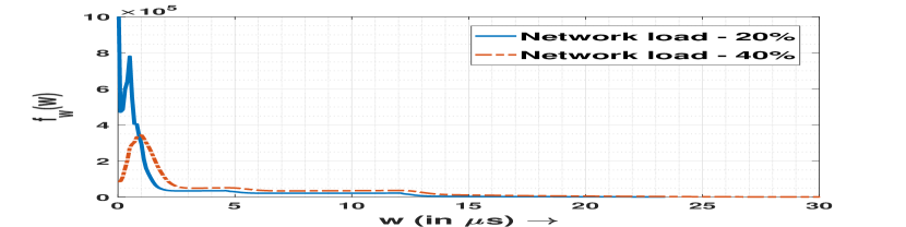
(a) Empirical pdfs of random queuing delays for TM-1 under 20% and 40% load.

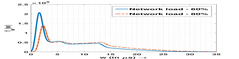
(b) Empirical pdfs of random queuing delays for TM-1 under 60% and 80% load.

Figure 1: Empirical pdfs of the random queuing delays for Traffic Model-1 under various loads.

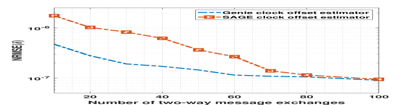
(a) NRMSE of clock offset for TM-1 under 60% load.

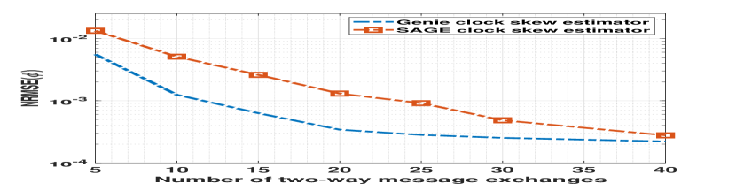
(b) NRMSE of clock skew for TM-1 under 60% load.

Figure 2: NRMSE of clock skew and offset for the considered CSOE schemes under Traffic Model-1.

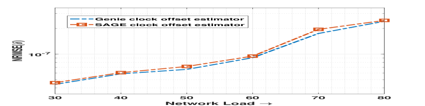
(a) NRMSE of clock offset for $P=100$.

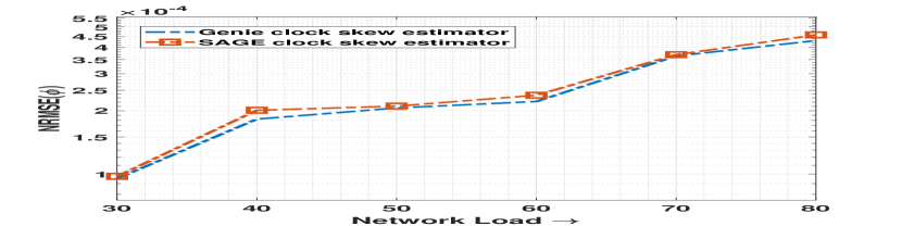
(b) NRMSE of clock skew for $P=40$.

Figure 3: NRMSE of clock offset and skew for the considered CSOE schemes under Traffic Model-1 under different loads.

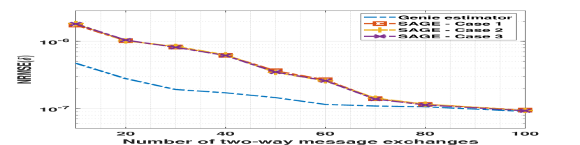
(a) NRMSE of clock offset for TM-1 under 60% load

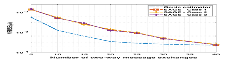
(b) NRMSE of clock skew for TM-1 under 60% load

Figure 4: NRMSE of clock offset and skew for different values of $\{\phi,\delta\}$ under Traffic Model-1. We have for case 1, $\{\phi,\delta\}=\{1.01,1~{}\mu s\}$, for case 2, $\{\phi,\delta\}=\{1.01,0~{}\mu s\}$ and for case 3, $\{\phi,\delta\}=\{1,0~{}\mu s\}$.

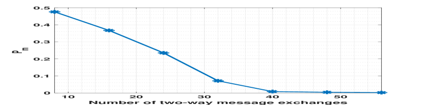
(a) Probability of miss detection for TM-1 under 60% load.

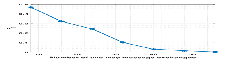
(b) Probability of false alarm detection for TM-1 under 60% load.

Figure 5: Probability of miss detection and probability of false alarm for TM-1 under 60% load.

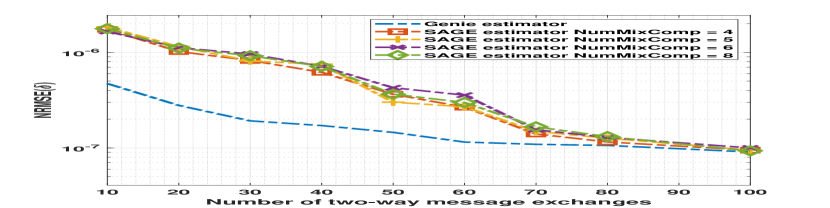
(a) NRMSE of clock offset for TM-1 under 60% load

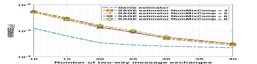
(b) NRMSE of clock skew for TM-1 under 60% load

Figure 6: NRMSE of clock offset and skew for different values of number of mixing components for the Gaussian mixture model.

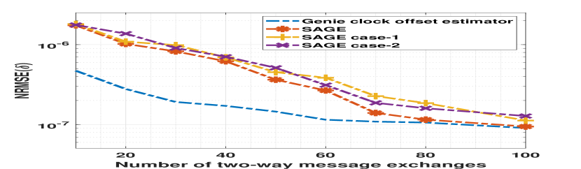
(a) NRMSE of clock offset for TM-1 under 60% load.

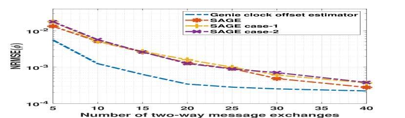
(b) NRMSE of clock skew for TM-1 under 60% load.

Figure 7: NRMSE of clock offset and skew for different cases. The samples $\bm{w}$ are assumed to be generated from a pdf corresponding to TM-1 under 60% load. In SAGE, $\tilde{\bm{w}}_{k}$ is has a pdf corresponding to TM-1 under 60% load (ideal scenario). In SAGE case-1, $\tilde{\bm{w}}_{k}$ is has a pdf corresponding to TM-1 under 50% load. In SAGE case-2, $\tilde{\bm{w}}_{k}$ is has a pdf corresponding to TM-1 under 70% load.

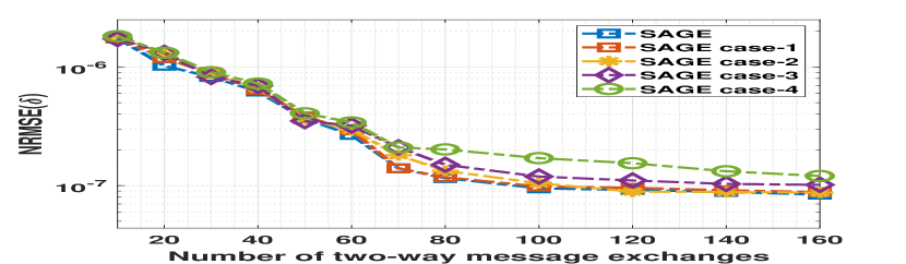
(a) NRMSE of clock offset for TM-1 under 60% load.

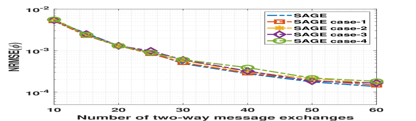
(b) NRMSE of clock skew for TM-1 under 60% load.

Figure 8: NRMSE of clock offset and skew for different cases. For SAGE, we assumed the parameters from the previous synchronization interval are estimated perfectly. In SAGE case-1, the common standard deviation of the estimates of $\delta,d_{i}^{ms},d_{i}^{sm}$ is fixed at $1.01\times 10^{-7}$, while the standard deviation of the estimates of $\phi$ is set to $1.01\times 10^{-4}$. In SAGE case-2, the common standard deviation of the estimates of $\delta,d_{i}^{ms},d_{i}^{sm}$ is fixed at $2.02\times 10^{-7}$, while the standard deviation of the estimates of $\phi$ is set to $2.02\times 10^{-4}$. In SAGE case-3, the common standard deviation of the estimates of $\delta,d_{i}^{ms},d_{i}^{sm}$ is fixed at $4.04\times 10^{-7}$, while the standard deviation of the estimates of $\phi$ is set to $4.04\times 10^{-4}$. In SAGE case-4, the common standard deviation of the estimates of $\delta,d_{i}^{ms},d_{i}^{sm}$ is fixed at $8.08\times 10^{-7}$, while the standard deviation of the estimates of $\phi$ is set to $8.08\times 10^{-4}$.

V Simulation Results

In this section, we compare the performance of the proposed robust clock skew and offset estimator to the performance lower bounds via numerical simulations. We consider the LTE backhaul network scenario described in Section I for packet-swtiched networks without synchronous ethernet. PTP is the primary synchronization option for operators with packet-switched backhaul networks that do not support SyncE [42, 43]. For simplicity, we assume $f_{{1i}}(.)=f_{{2i}}(.)=f_{{w}}(.)$ for $i=1,2,\cdots,N$. However, the proposed algorithm does not assume that all the pdfs are the same. Further, we assume the deterministic path delays are identical across all the master-slave communication paths, i.e., $d_{1}=d_{2}=\cdots=d_{N}=d$, where $d$ denotes an unknown deterministic path delay parameter. We first briefly describe the approach used to generate the random queuing delays in our simulations.

V-A Generation of the random queuing delays

We follow the approach given in [9] for generating the random queuing delays in LTE backhaul networks. We consider a Gigabit Ethernet network consisting of a cascade of $10$ switches between the master and slave nodes. A two-class non-preemptive priority queue is used to model the traffic at each switch. The network traffic at the switch is comprised of the lower priority background traffic and the higher priority synchronization messages. We assume cross-traffic flows, where new background traffic is injected at each switch and this traffic exits at the subsequent switch. The arrival times and size of background traffic packets injected at each switch are assumed to be statistically independent. We use Traffic Model 1 (TM-1) from the ITU-T specification G.8261 [31] for generating the background traffic at each switch. The interarrival times between packets in background traffic are assumed to follow an exponential distribution, and we set the rate parameter of each exponential distribution accordingly to obtain the desired load factor, i.e., the percentage of the total capacity consumed by background traffic[9]. The empirical pdf of the PDV in the backhaul networks was obtained in [9] for different load factors and are shown in 1. The timestamps $t_{1ij}$ and $t_{4ij}$ are set to $60j$ $\mu s$ and $60j$ $\mu s+30\mu s$, respectively, for $i=1,\cdots,N$ and $j=0,1,\cdots,P-1$. For a given value of parameters, the timestamps $t_{2ij}$ and $t_{3ij}$ are then generated using (1).

V-B Numerical results

In our results, we use the $\mbox{NRMSE}(\hat{\delta})=\sqrt{\mbox{NMSE}(\hat{\delta})}$ and $\mbox{NRMSE}(\hat{\phi})=\sqrt{\mbox{NMSE}(\hat{\phi})}$ metrics defined in (13) for evaluating the performance of the considered CSOE schemes. We evaluate the NRMSE performance of the clock skew and offset estimate obtained from the SAGE-CSOE scheme described in Section IV and compare it against the NRMSE performance of the genie optimum estimator of $\delta$ and $\phi$ calculated using (15) and (16), respectively. In our numerical results presented in Figures 2-7, we approximate the multidimensional integrals in (15) and (16) with Riemann summations. We approximate the integral over $\mathbb{R}^{+}$ (corresponding to $\phi$) using Riemann sums by setting the width of the Riemann summation bins to $0.001$ and the limits of the integral to $[0.5,2]$ and the integral over $\mathbb{R}$ (corresponding to $\delta$, $d_{i}$ and $\tau_{i}$) is approximated using Riemann sums by setting the width of the Riemann summation bins to $0.01$ $\mu s$ and the limits of the integral to $[-10\mu s,10\mu s]$. We tried smaller bin-widths and observed from the results that the calculation were quite accurate. We assume the availability of $N=3$ master-slave communication paths with one path having an unknown asymmetry between the deterministic path delays. The values of $\phi$ and $\delta$ are fixed to $1.01$ and $1~{}\mu s$, respectively. The value of $d$ is set as $1~{}\mu s$, i.e., $d_{1}=d_{2}=d_{3}=d=1~{}\mu s$. For the master-slave communication path with an unknown asymmetry, we set the value of $\tau_{i}$ to $4~{}\mu s$. The user-defined parameter $d_{\tau}$ is set to $2~{}\mu s$. The number of mixture components used in the GMM approximation is set to $4$, and the value of $P_{t}$ is fixed as $P$, where $P$ is the number of two-way message exchanges used in the calculation of $\delta$ and $\phi$. Some key observations from the results are listed below:

1. Performance of the robust CSOE schemes: The NRMSE performance of the proposed robust iterative CSOE scheme against the NRMSE of the optimum estimator is presented in Figures 2 and 3. In Figure 2, we observe that the performance of the robust iterative SAGE-CSOE scheme improves with an increase in the number of two-way message exchanges, $P$, and exhibits performance close to the genie optimum estimator for a sufficiently large number of two-way message exchanges. As expected, the optimum estimators exhibits the smallest NRMSE due to prior information on which of the master-slave communication paths have unknown deterministic path asymmetry as well as the complete information regarding $f_{w}(.)$. In Figure 3, we evaluate the performance of the robust scheme for TM-1 under different loads for a fixed value of $P$. We observe that the proposed robust clock skew and offset estimation scheme exhibits a performance close to the NRMSE of the optimum estimators for various network scenarios.

2. Performance comparison for different values of clock skew and offset: Figure 4 shows us the performance of the robust iterative SAGE-CSOE scheme for different values of $\phi$ and $\delta$. The performance lower bounds from Proposition 1 are independent of the parameter values as is any invariant estimation scheme (see Chapter 6, [24]). From the results, we also observe that the NRMSE performance of the SAGE-CSOE appears to be nearly independent of the parameter values in the cases shown.

3. Probability of miss detection ($P_{m}$) and probability of false alarm ($P_{f}$): Let $\hat{\pi}_{i}^{(s)}$ denote the estimate of $\pi_{i}$ (for $i=1,2,\cdots,N$) obtained from the SAGE algorithm after convergence. The $i^{\mbox{th}}$ master-slave communication path is declared as asymmetric if $\hat{\pi}_{i}^{(s)}\geq 0.5$, else the $i^{\mbox{th}}$ master-slave communication path is declared as symmetric. We define the probability of miss detection (denoted by $P_{m}$) as the probability of identifying an asymmetric master-slave communication path as being symmetric, while the probability of false alarm (denoted by $P_{f}$) is defined as the probability of identifying a symmetric master-slave communication path as asymmetric. Figure 5 shows us the $P_{m}$ and $P_{f}$ for the SAGE-CSOE scheme for different values of two-way message exchanges. As expected, $P_{m}$ and $P_{f}$ decrease to $0$ as we increase the number of two-way messages exchanges used.

4. Performance comparison for different values of number of GMM components: Figure 6 shows us the performance of the proposed SAGE algorithm for a different number of mixing components in the GMM. As seen from the results, there is no noticeable degradation in the performance of the SAGE CSOE scheme, possibly indicating that the performance of the algorithm is relatively robust against over-fitting.

5. Performance when the pdf of $\tilde{\bm{w}}_{k}$ is different than the pdf of $\bm{w}_{k}$: In certain scenarios, the pdf of $\tilde{\bm{w}}_{k}$ for $k=1,2$ may be slightly different from the pdf of $\bm{w}_{k}$ for $k=1,2$. This could be a result of some network conditions slowly changing with time across different blocks of two-way message exchanges (what we called windows). Figure 7 shows us the performance of the proposed algorithm for this scenario. We observe a slight degradation in the performance of the algorithm compared to the scenario when the pdf of $\tilde{\bm{w}}_{k}$ is identical to $\bm{w}_{k}$. However, as the number of two-way message exchanges is increased, the performance of the algorithm improves indicating that the algorithm is relatively robust against slowly changing network conditions with a sufficient number of two-way exchanges.

6. Inaccurate previous synchronization parameters: We now consider the scenario where $\phi$, $d_{i}^{ms}$, $d_{i}^{sm}$ and $\delta$ from the previous synchronization window are inaccurate and model them as Gaussian random variables with the mean being the true values of $1.01$, $1~{}\mu s$, $1~{}\mu s$ and $1~{}\mu s$, respectively. The common standard deviation of $d_{i}^{ms}$, $d_{i}^{sm}$ and $\delta$ from the last synchronization is varied from $1.01\times 10^{-7}$ to $8.08\times 10^{-7}$, while the standard deviation of $\phi$ is varied from $1.01\times 10^{-4}$ to $8.08\times 10^{-4}$. Figure 8 shows the performance of the proposed CSOE scheme. From the results, we observe a noticeable degradation in the performance of the robust CSOE scheme, especially for larger values of the standard deviations of $\phi$, $d_{i}^{ms}$, $d_{i}^{sm}$ and $\delta$ from the previous synchronization window. However, the performance improves with an increasing number of two-way message exchanges and is close to the case where the parameters are known perfectly for a sufficiently large number of message exchanges.

VI Conclusion

In this paper, assuming the availability of multiple master-slave communication paths, we have developed useful lower bounds on the skew normalized mean square estimation error for a clock skew and offset estimation scheme in the presence of unknown path asymmetries. Also, we developed a robust iterative clock skew and offset estimation scheme that employs the SAGE algorithm for jointly estimating the clock skew and offset. The robust iterative clock skew and offset estimation scheme has low computational complexity and does not require the complete information regarding the statistical distributions of the queuing delays. The robust scheme exhibits a skew normalized mean square estimation error close to our performance lower bounds in several network scenarios. Furthermore, a number of time synchronization protocols including NTP[2], TPSN [3], LTS [4], and RBS [5] are built on message exchanges. The proposed robust iterative scheme can be easily modified for these protocols.

Appendix A Proof of Proposition 1

Proof.

Here we present the beautiful and complicated invariant decision theory from [24, 44] in a simple way to present our proof. In [24, 44], it was shown that the right invariant prior, $\pi^{r}(.)$, on ${\mathcal{G}}_{M}$ from (9) is obtained by finding the function that satisfies $\int_{\mathcal{A}}\pi^{r}(\bm{\theta})d\bm{\theta}=\int_{\mathcal{A}_{0}^{(r)}}\pi^{r}(\bm{\theta}_{0}^{(r)})d\bm{\theta}_{0}^{(r)}$ for all $\mathcal{A}\subseteq\bm{\Theta}$, for all $\bar{g}_{\phi,\bm{\gamma},{\delta}}(.)\in\bar{\mathcal{G}}_{M}$ and for all $\bm{\theta}_{0}=(\phi_{0},\bm{\gamma}_{0},{\delta}_{0})\in\bm{\Theta}$. The variables $\mathcal{A}_{0}^{(r)}$ and $\bm{\theta}_{0}^{(r)}$ are defined as follows:

$$\mathcal{A}_{0}^{(r)} =\{\bm{\theta}_{0}^{(r)}=\left(\phi_{0}^{(r)},\bm{\gamma}_{0}^{(r)},{\delta}_{0}^{(r)}\right):\bm{\theta}_{0}^{(r)}=\bar{g}_{\phi,\bm{\gamma},{\delta}}(\bm{\theta}_{0}),(\phi,\bm{\gamma},{\delta})\in\mathcal{A}\},$$ (37)

$$=\{\bm{\theta}_{0}^{(r)}=(\phi\phi_{0},\bm{\gamma}_{0}+\bm{\gamma}/\phi_{0},\phi{\delta}_{0}+{\delta}):(\phi,\bm{\gamma},{\delta})\in\mathcal{A}\}.$$ (38)

The right invariant prior for $\bar{\mathcal{G}}_{M}$ is given by $\pi^{r}(\bm{\theta})=\phi^{N+K-1}$. To see this, note that (from change of variables)

$$\int_{\mathcal{A}}\phi^{N+K-1}d\bm{\theta} =\int_{\mathcal{A}_{0}^{(r)}}\left(\frac{\phi_{0}^{(r)}}{\phi_{0}}\right)^{N+K-1}\frac{d\bm{\theta}}{d\bm{\theta}_{0}^{(r)}}d\bm{\theta}_{0}^{(r)}=\int_{\mathcal{A}_{0}^{(r)}}(\phi_{0}^{(r)})^{N+K-1}d\bm{\theta}_{0}^{(r)},$$ (39)

since the Jacobian of the transformation in (38) is given by

$$\frac{d\bm{\theta}_{0}^{(r)}}{d\bm{\theta}} =\det\left(\begin{bmatrix}\frac{\partial\phi_{0}^{(r)}}{\partial\phi}&\frac{\partial\phi_{0}^{(r)}}{\partial\bm{\gamma}}&\frac{\partial\phi_{0}^{(r)}}{\partial{\delta}}\\ \frac{\partial\bm{\gamma}_{0}^{(r)}}{\partial\phi}&\frac{\partial\bm{\gamma}_{0}^{(r)}}{\partial\bm{\gamma}}&\frac{\partial\bm{\gamma}_{0}^{(r)}}{\partial{\delta}}\\ \frac{\partial{\delta}_{0}^{(r)}}{\partial\phi}&\frac{\partial{\delta}_{0}^{(r)}}{\partial\bm{\gamma}}&\frac{\partial{\delta}_{0}^{(r)}}{\partial{\delta}}\\ \end{bmatrix}\right)=\det\left(\begin{bmatrix}\phi_{0}&\bm{0}_{N+K}^{T}&0\\ \bm{0}_{N+K}&\frac{1}{\phi_{0}}\bm{I}_{N+K}&\bm{0}_{N+K}\\ {\delta}_{0}&\bm{0}_{N+K}^{T}&1\end{bmatrix}\right)=\frac{1}{\phi_{0}^{N+K-1}}.$$

A optimum invariant estimator of $\delta$ under $\mathcal{G}_{M}$ from (9), denoted by $\hat{\delta}_{opt}$, can now be obtained by solving [24, 44]

$$\hat{\delta}_{opt}(\bm{y})=\operatorname*{\arg\min}_{\hat{\delta}}\int_{\bm{\Theta}}\frac{(\hat{\delta}(\bm{y})-\delta)^{2}}{\phi^{2}}\pi^{r}(\bm{\theta}|\bm{y})d\bm{\theta},$$ (40)

where $\pi^{r}(\bm{\theta}|\bm{y})=\frac{f(\bm{y}|\bm{\theta})\pi^{r}(\bm{\theta})}{\int_{\bm{\Theta}}f(\bm{y}|\bm{\theta})\pi^{r}(\bm{\theta})d\bm{\theta}}$ and $\pi^{r}(\bm{\theta})$ is the right invariant prior corresponding to $\bar{\mathcal{G}}_{M}$. To find $\hat{\delta}_{opt}$, we differentiate the objective function in (40) with respect to $\hat{\delta}(\bm{y})$, set the result equal to zero and solve for $\hat{\delta}(\bm{y})$. We have

$$\hat{\delta}_{opt}(\bm{y}) =\frac{\int_{\bm{\Theta}}\frac{\delta}{\phi^{2}}\pi^{r}(\bm{\theta}|\bm{y})d\bm{\theta}}{\int_{\bm{\Theta}}\frac{1}{\phi^{2}}\pi^{r}(\bm{\theta}|\bm{y})d\bm{\theta}} =\frac{\int_{\bm{\Theta}}\frac{\delta}{\phi^{2}}f(\bm{y}|\bm{\theta})\pi^{r}(\bm{\theta})d\bm{\theta}}{\int_{\bm{\Theta}}\frac{1}{\phi^{2}}f(\bm{y}|\bm{\theta})\pi^{r}(\bm{\theta})d\bm{\theta}}=\frac{\int_{\mathbb{R}^{+}}\int_{\mathbb{R}^{N+K+1}}\frac{\delta\Gamma_{1}(\phi,\delta,\bm{d},\bm{\tau},\bm{y})\Gamma_{0}(\phi,\delta,\bm{d},\bm{y})}{\phi^{2NP-N-K+3}}d\bm{\tau}d(\bm{d})d\delta d\phi}{\int_{\mathbb{R}^{+}}\int_{\mathbb{R}^{N+K+1}}\frac{\Gamma_{1}(\phi,\delta,\bm{d},\bm{\tau},\bm{y})\Gamma_{0}(\phi,\delta,\bm{d},\bm{y})}{\phi^{2NP-N-K+3}}d\bm{\tau}d(\bm{d})d\delta d\phi},$$ (41)

where $\Gamma_{1}(\phi,\delta,\bm{d},\bm{\tau},\bm{y})$ and $\Gamma_{0}(\phi,\delta,\bm{d},\bm{y})$ are defined in Proposition 1. Using a similar derivative-based approach, we obtain $\hat{\phi}_{opt}(\bm{y})$ defined in Proposition 1. ∎

Appendix B Outline of Derivation of Update Equations

The first step in the EM algorithm is the specification of a set of “complete data” $\bm{X}_{c}$ and “incomplete data” $\bm{X}$ for the problem [29, 28]. The pdf’s for $\bm{X}$ and $\bm{X}_{c}$ are characterized by a set of common parameters $\bm{\Phi}$. The complete data is not available, but it is chosen in such a way so that if it were available, then the MLE of $\bm{\Phi}$ would be easy to find. The EM algorithm addresses this situation and provides an iterative procedure for the maximum likelihood estimation of $\bm{\Phi}$ based on the incomplete data $\bm{X}$. The SAGE algorithm [30] is closely related to the EM algorithm, except that the parameter set is partitioned into subsets $\bm{\Phi}_{1},\bm{\Phi}_{2},\cdots,\bm{\Phi}_{M}$ with $\bm{\Phi}=\bm{\Phi}_{1}\bigcup\bm{\Phi}_{2}\cdots\bigcup\bm{\Phi}_{M}$. Then, on each iteration, $\bm{\Phi}_{1}$ is updated with $\bm{\Phi}_{2},\cdots,\bm{\Phi}_{M}$ fixed, followed by the update of $\bm{\Phi}_{2}$ with $\bm{\Phi}_{1},\cdots,\bm{\Phi}_{M}$ fixed and so on. The sequence of estimates produced by the SAGE algorithm has non-decreasing likelihood for the incomplete data [30]. In this paper, we apply the SAGE algorithm to the considered problem. The SAGE algorithm update equations are derived as follows. The parameter set to be estimated is $\bm{\Omega}_{\pi}=[\phi,\delta,d_{1},\cdots,d_{N},\tau_{1},\cdots,\tau_{N},\bm{\pi},\bm{\alpha}_{1},\cdots,\allowbreak\bm{\alpha}_{N},\bm{\beta}_{1},\cdots,\bm{\beta}_{N},\bm{\mu}_{11},\allowbreak\cdots,\bm{\mu}_{1N},\bm{\sigma}_{11},\cdots,\bm{\sigma}_{1N},\allowbreak\bm{\mu}_{21},\cdots,\bm{\mu}_{2N},\bm{\sigma}_{21},\allowbreak\cdots,\bm{\sigma}_{2N}]$. The number of mixture components in the forward and reverse path, denoted by $M_{i}$ and $L_{i}$, respectively, are assumed to be fixed for $i=1,2,\cdots,N$. The incomplete data set $\bm{X}$ consists of the observed timestamps

$$\bm{X} =\{t_{1ij},t_{2ij},t_{3ij},t_{4ij},\tilde{w}_{1ij_{t}},\tilde{w}_{2ij_{t}}:i=1,2,\cdots,N,j=1,2,\cdots,P,j_{t}=1,2,\cdots,P_{t}\}$$ (42)

from (1). The complete data set, denoted by $\bm{X}_{c}$, is defined as

$$\bm{X}_{c} =\{t_{1ij},(t_{2ij},z_{ij},r_{ij}),(t_{3ij},s_{ij}),t_{4ij},(\tilde{w}_{1ij_{t}},\tilde{r}_{ij}),(\tilde{w}_{2ij_{t}},\tilde{s}_{ij}):i=1,2,\cdots,N,j=1,2,\cdots,P,$$

$$j_{t}=1,2,\cdots,P_{t}\}$$ (43)

where $z_{ij}\in\{0,1\}$ identifies whether the $j^{th}$ two-way message exchange at the $i^{th}$ path has an unknown path asymmetry, $r_{ij}\in\{1,2,\cdots,M_{i}\}$ identifies which term in the mixture pdf approximation of $f_{1i}(.)$ in (17) produced the random queuing sample in the forward path time stamps $t_{2ij}$, and $s_{ij}\in\{1,2,\cdots,L_{i}\}$ identifies which term in the mixture pdf approximation of $f_{2i}(.)$ in (17) produced the random queuing sample in the reverse path time stamps $t_{3ij}$. Similarly, $\tilde{r}_{ij}\in\{1,2,\cdots,M_{i}\}$ and $\tilde{s}_{ij}\in\{1,2,\cdots,L_{i}\}$ identifies which term in the mixture pdf produced the random queuing samples $\tilde{w}_{1ij}$ and $\tilde{w}_{2ij}$, respectively. The definition of the complete data for mixture models is discussed in [29]. The incomplete data log likelihood is given in (IV-A) and the complete data log likelihood, denoted by $\mathcal{L}_{com}({\bm{\Omega}}_{\pi}|\bm{X}_{c})$, is defined in (44) as

$$\sum_{i=1}^{N}\sum_{j=1}^{P}z_{ij}\ln\left[\pi_{i}\alpha_{r_{ij}}\mathcal{P}_{\mu_{1r_{ij}},\sigma_{1r_{ij}}}\left(\frac{t_{2ij}-\delta}{\phi}-d_{i}-\tau_{i}-t_{1ij}\right)\beta_{s_{ij}}\mathcal{P}_{\mu_{2s_{ij}},\sigma_{2s_{ij}}}\left(t_{4ij}-d_{i}+\frac{\delta-t_{3ij}}{\phi}\right)\right]$$

$$+(1-z_{ij})\ln\left[(1-\pi_{i})\alpha_{r_{ij}}\mathcal{P}_{\mu_{1r_{ij}},\sigma_{1r_{ij}}}\left(\frac{t_{2ij}-\delta}{\phi}-d_{i}-t_{1ij}\right)\beta_{s_{ij}}\mathcal{P}_{\mu_{2s_{ij}},\sigma_{2s_{ij}}}\left(t_{4ij}-d_{i}+\frac{\delta-t_{3ij}}{\phi}\right)\right]$$

$$-2NP\ln\phi+\sum_{i=1}^{N}\sum_{j=1}^{P_{t}}\ln\left[\alpha_{\tilde{r}_{ij}}\mathcal{P}_{\mu_{1\tilde{r}_{ij}},\sigma_{1\tilde{r}_{ij}}}\left(\tilde{w}_{1ij}\right)\right.\left.\beta_{\tilde{s}_{ij}}\mathcal{P}_{\mu_{2\tilde{s}_{ij}},\sigma_{2\tilde{s}_{ij}}}\left(\tilde{w}_{2ij}\right)\right].$$ (44)

We now describe the steps of the EM algorithm. The E-step of the EM algorithm performs an average over the unavailable parts of the complete data conditioned on the incomplete data and current parameter estimates $\hat{\bm{\Omega}}_{\pi}^{{}^{\prime}}$ as in $Q(\bm{\Omega}_{\pi}|\hat{\bm{\Omega}}_{\pi}^{{}^{\prime}})=E\left\{\mathcal{L}_{com}({\bm{\Omega}}_{\pi}|\bm{X}_{c})\bigg{|}\bm{X},\hat{\bm{\Omega}}_{\pi}^{{}^{\prime}}\right\}$

$$= \sum_{i=1}^{N}\sum_{j=1}^{P}\sum_{k=1}^{M_{i}}\sum_{l=1}^{L_{i}}\chi^{(1)}_{ijkl}\ln\bigg{[}\pi_{i}\alpha_{ik}\mathcal{P}_{\mu_{1ik},\sigma_{1ik}}\left(\frac{t_{2ij}-\delta}{\phi}-d_{i}-\tau_{i}-t_{1ij}\right)\left.\beta_{il}\mathcal{P}_{\mu_{2il},\sigma_{2il}}\left(t_{4ij}-d_{i}+\frac{\delta-t_{3ij}}{\phi}\right)\right]$$

$$+\chi^{(0)}_{ijkl}\ln\left[(1-\pi_{i})\alpha_{ik}\mathcal{P}_{\mu_{1ik},\sigma_{1ik}}\left(\frac{t_{2ij}-\delta}{\phi}-d_{i}-t_{1ij}\right)\right.\left.\beta_{il}\mathcal{P}_{\mu_{2il},\sigma_{2il}}\left(t_{4ij}-d_{i}+\frac{\delta-t_{3ij}}{\phi}\right)\right]$$

$$+\sum_{i=1}^{N}\sum_{j=1}^{P_{t}}\sum_{k=1}^{M_{i}}\sum_{l=1}^{L_{i}}\tilde{a}_{ijkl}\ln\Big{[}\alpha_{ik}\mathcal{P}_{\mu_{1ik},\sigma_{1ik}}\left(\tilde{w}_{1ij}\right)\beta_{il}\mathcal{P}_{\mu_{2il},\sigma_{2il}}\left(\tilde{w}_{2ij}\right)\Big{]}-2NP\ln\phi,$$ (45)

where $\chi_{ijkl}^{(1)},\chi_{ijkl}^{(0)},\tilde{a}_{ijkl}$ are defined in (23), (24) and (25), respectively. The EM algorithm [45] updates the parameter estimates $\hat{\bm{\Omega}}_{\pi}^{{}^{\prime}}$ to new values $\hat{\bm{\Omega}}_{\pi}$ that maximize $Q(\bm{\Omega}_{\pi}|\hat{\bm{\Omega}}_{\pi}^{{}^{\prime}})$ in (45). This is called the M-step of the EM algorithm, and the updated parameters are guaranteed to not decrease the incomplete data likelihood, defined in (IV-A). The SAGE algorithm inherits this property. The parameter set $\bm{\Omega}_{\pi}$ is partitioned into the following subsets: $\bm{\Omega}_{\pi,1}=\{\bm{\pi},\bm{\alpha}_{1},\cdots,\bm{\alpha}_{N},\bm{\beta}_{1},\cdots,\bm{\beta}_{N}\}$, $\bm{\Omega}_{\pi,2}=\{\bm{\mu}_{11},\cdots,\bm{\mu}_{1N},\bm{\mu}_{21},\cdots,\bm{\mu}_{2N}\}$, $\bm{\Omega}_{\pi,3}=\{\bm{\sigma}_{11},\cdots,\bm{\sigma}_{1N},\bm{\sigma}_{21},\cdots,\bm{\sigma}_{2N}\}$, $\bm{\Omega}_{\pi,4}=\{d_{1},d_{2},\cdots,d_{N}\}$, $\bm{\Omega}_{\pi,5}=\{\tau_{1},\tau_{2},\cdots,\tau_{N}\}$, $\bm{\Omega}_{\pi,6}=\delta$, $\bm{\Omega}_{\pi,7}=\phi$. First, $Q(\bm{\Omega}_{\pi}|\hat{\bm{\Omega}}_{\pi}^{{}^{\prime}})$ is first maximized with respect to $\bm{\Omega}_{\pi,1}$ with all other parameters fixed at the current parameter estimates. Then, $\bm{\Omega}_{\pi,1}$ is set equal to the updated parameter estimate, after which, $Q(\bm{\Omega}_{\pi}|\hat{\bm{\Omega}}_{\pi}^{{}^{\prime}})$ is maximized with respect to $\bm{\Omega}_{\pi,2}$ with all other parameters fixed at the current parameter estimates. This procedure is repeated for all the parameter subsets $\bm{\Omega}_{\pi,1},\bm{\Omega}_{\pi,2},\cdots,\bm{\Omega}_{\pi,7}$ until the algorithm converges (small change in $Q(\bm{\Omega}_{\pi}|\hat{\bm{\Omega}}_{\pi}^{{}^{\prime}})$).

Appendix C Initialization of parameters for SAGE algorithm

As the objective function for the optimization problem in (21) is not necessarily convex, proper initialization of the various parameters is employed to promote convergence to the global minimum instead of local minimums. We present a simple ad-hoc scheme to obtain the initial values of the various parameters, denoted by $\hat{\bm{\Omega}}_{\pi}^{(0)}$ for the SAGE algorithm. The steps of the initialization are enumerated below:

1:  First, we define new variables $\gamma_{i}=(\phi(d_{i}+\tau_{i})+\delta)$ and $\zeta_{i}=(-\phi d_{i}+\delta)$ for $i=1,2,\cdots,N$.

2:  for $i=1:N$ do

3:     For a given value of $M_{i}$, run the EM algorithm for the GMM using the update equations given in [45] on $\tilde{\bm{w}}_{1i}$ to obtain $\hat{\alpha}_{ik}^{(0)}$, $\hat{\mu}_{1ik}^{(0)}$ and $\hat{\sigma}_{1ik}^{(0)}$.

4:     For a given value of $L_{i}$, run the EM algorithm for the GMM using the update equations given in [45] on $\tilde{\bm{w}}_{2i}$ to obtain $\hat{\beta}_{il}^{(0)}$, $\hat{\mu}_{2il}^{(0)}$ and $\hat{\sigma}_{2il}^{(0)}$.

5:     Using $\hat{\alpha}_{ik}^{(0)}$, $\hat{\mu}_{1ik}^{(0)}$ and $\hat{\sigma}_{1ik}^{(0)}$, construct an approximate pdf for $f_{1i}(.)$, denoted by $\tilde{f}_{1i}(.)$. Similarly, using $\hat{\beta}_{il}^{(0)}$, $\hat{\mu}_{2il}^{(0)}$ and $\hat{\sigma}_{2il}^{(0)}$, construct an approximate pdf for $f_{2i}(.)$, denoted by $\tilde{f}_{2i}(.)$.

6:     Consider the timestamps $\bm{t}_{1i}$ and $\bm{t}_{2i}$ from the $i^{\mbox{th}}$ master-slave communication path. We know $\bm{t}_{2i}=(\bm{t}_{1i}+\bm{w}_{1i})\phi+\gamma_{i}\mathds{1}_{P}$. Relaxing the dependency of $\gamma_{i}$ on $\phi$, we use the optimum CSOE scheme proposed in [19] to obtain an estimate of $\phi$ and $\gamma_{i}$, denoted by $\hat{\phi}_{fwd,i}$ and $\hat{\gamma}_{i}$ respectively.

7:     Consider the timestamps $\bm{t}_{3i}$ and $\bm{t}_{4i}$ from the $i^{\mbox{th}}$ master-slave communication path. We have $\bm{t}_{3i}=(\bm{t}_{4i}-\bm{w}_{2i})\phi+\zeta_{i}\mathds{1}_{P}$. Relaxing the dependency of $\zeta_{i}$ on $\phi$, we use the optimum CSOE scheme in [19] to obtain an estimate of $\phi$ and $\zeta_{i}$, denoted by $\hat{\phi}_{rev,i}$ and $\hat{\zeta}_{i}$ respectively.

8:     We then construct the estimate of the clock skew from the timestamps exchanged in the $i^{\mbox{th}}$ master-slave communication path, denoted by $\hat{\phi}_{i}$, as $\hat{\phi}_{i}=(\hat{\phi}_{fwd,i}+\hat{\phi}_{rev,i})/2$. Similarly, we calculate an estimate of $\delta$, denoted by $\hat{\delta}_{i}$, from the timestamps exchanged in the $i^{\mbox{th}}$ master-slave communication path as $\hat{\delta}_{i}=(\hat{\gamma}_{i}+\hat{\zeta}_{i})/2$.

9:  end for

10:  Using the obtained estimates $\hat{\phi}_{i}$ and $\hat{\delta}_{i}$ for $i=1,2,\cdots,N$, we fix our initial estimate of $\delta$, denoted by $\hat{\delta}^{(0)}$, as $\hat{\delta}^{(0)}=\mbox{median}\{\hat{\delta}_{1},\hat{\delta}_{2},\cdots,\hat{\delta}_{N}\}$. Similarly, we fix our initial estimate of $\phi$, denoted by $\hat{\phi}^{(0)}$, as $\hat{\phi}^{(0)}=\mbox{mean}\{\hat{\phi}_{1},\hat{\phi}_{2},\cdots,\hat{\phi}_{N}\}$.

11:  for $i=1:N$ do

12:     Estimate the total deterministic path delay in the forward path of the $i^{\mbox{th}}$ master-slave communication path as $\hat{d}_{fwd,i}=(\hat{\gamma}_{i}-\hat{\delta}^{(0)})/\hat{\phi}^{(0)}$. Similarly, estimate the total deterministic path delay in the reverse path of the $i^{\mbox{th}}$ master-slave communication path as $\hat{d}_{rev,i}=(\hat{\delta}^{(0)}-\hat{\zeta}_{i})/\hat{\phi}^{(0)}$.

13:     Set $\hat{\pi}_{i}^{(0)}$ as $\frac{e^{\left(|\hat{d}_{fwd,i}-\hat{d}_{rev,i}|-d_{\tau}\right)\kappa}}{e^{\left(|\hat{d}_{fwd,i}-\hat{d}_{rev,i}|-d_{\tau}\right)\kappa}+1}$, where $\kappa$ is a normalization constant.

14:     if $\left|\hat{d}_{fwd,i}-\hat{d}_{rev,i}\right|\leq d_{\tau}$ then

15:        Set $\hat{d}_{i}^{(0)}$ to to $(\hat{d}_{fwd,i}+\hat{d}_{rev,i})/2$ and $\hat{\tau}_{i}^{(0)}$ to $0$.

16:     else

17:        Set $\hat{d}_{i}^{(0)}$ to to $\hat{d}_{rev,i}$ and $\hat{\tau}_{i}^{(0)}$ to $(\hat{d}_{fwd,i}-\hat{d}_{rev,i})$.

18:     end if

19:  end for

References

- [1] IEEE, “IEEE Standard for a Precision Clock Synchronization Protocol for Networked Measurement and Control Systems,” IEEE Std 1588-2008 (Revision of IEEE Std 1588-2002), pp. 1–300, July 2008.
- [2] D. L. Mills, “Internet time synchronization: the network time protocol,” IEEE Transactions on Communications, vol. 39, no. 10, pp. 1482–1493, Oct 1991.
- [3] S. Ganeriwal, R. Kumar, and M. B. Srivastava, “Timing-sync Protocol for Sensor Networks,” in Proceedings of the 1st International Conference on Embedded Networked Sensor Systems, ser. SenSys ’03. New York, NY, USA: ACM, 2003, pp. 138–149.
- [4] J. Van Greunen and J. Rabaey, “Lightweight Time Synchronization for Sensor Networks,” in Proceedings of the 2Nd ACM International Conference on Wireless Sensor Networks and Applications, ser. WSNA ’03. New York, NY, USA: ACM, 2003, pp. 11–19.
- [5] J. Elson, L. Girod, and D. Estrin, “Fine-grained network time synchronization using reference broadcasts,” SIGOPS Oper. Syst. Rev., vol. 36, no. SI, pp. 147–163, Dec. 2002. [Online]. Available: http://doi.acm.org/10.1145/844128.844143
- [6] K. L. Noh, Q. M. Chaudhari, E. Serpedin, and B. W. Suter, “Novel Clock Phase Offset and Skew Estimation Using Two-Way Timing Message Exchanges for Wireless Sensor Networks,” IEEE Transactions on Communications, vol. 55, no. 4, pp. 766–777, April 2007.
- [7] Q. M. Chaudhari, E. Serpedin, and K. Qaraqe, “On Maximum Likelihood Estimation of Clock Offset and Skew in Networks With Exponential Delays,” IEEE Transactions on Signal Processing, vol. 56, no. 4, pp. 1685–1697, April 2008.
- [8] Y. C. Wu, Q. Chaudhari, and E. Serpedin, “Clock Synchronization of Wireless Sensor Networks,” IEEE Signal Processing Magazine, vol. 28, no. 1, pp. 124–138, Jan 2011.
- [9] A. Guruswamy, R. S. Blum, S. Kishore, and M. Bordogna, “Minimax Optimum Estimators for Phase Synchronization in IEEE 1588,” IEEE Transactions on Communications, vol. 63, no. 9, pp. 3350–3362, Sept 2015.
- [10] G. Gaderer, T. Sauter, and G. Bumiller, “Clock Synchronization in Powerline Networks,” in International Symposium on Power Line Communications and Its Applications, 2005., April 2005, pp. 71–75.
- [11] I. Hadvzic, D. R. Morgan, and Z. Sayeed, “A Synchronization Algorithm for Packet MANs,” IEEE Transactions on Communications, vol. 59, no. 4, pp. 1142–1153, April 2011.
- [12] “IEEE Standard Profile for Use of IEEE 1588 Precision Time Protocol in Power System Applications,” IEEE Std. C37.238-2011, July 2011.
- [13] K. Harris, “An application of IEEE 1588 to Industrial Automation,” in 2008 IEEE International Symposium on Precision Clock Synchronization for Measurement, Control and Communication, Sept 2008, pp. 71–76.
- [14] N. M. Freris, S. R. Graham, and P. R. Kumar, “Fundamental Limits on Synchronizing Clocks Over Networks,” IEEE Transactions on Automatic Control, vol. 56, no. 6, pp. 1352–1364, June 2011.
- [15] M. Ullmann and M. Vögeler, “Delay attacks — implication on ntp and ptp time synchronization,” in 2009 International Symposium on Precision Clock Synchronization for Measurement, Control and Communication, Oct 2009, pp. 1–6.
- [16] H. Balakrishnan, V. Padmanabhan, G. Fairhurst, and M. Sooriyabandara, “TCP performance implications of network path asymmetry,” Tech. Rep. RFC 3449, Sept. 2002.
- [17] A. K. Karthik and R. S. Blum, “Estimation Theory-Based Robust Phase Offset Determination in Presence of Possible Path Asymmetries,” IEEE Transactions on Communications, vol. 66, no. 4, pp. 1624–1635, April 2018.
- [18] A. K. Karthik and R. S. Blum, “Robust phase offset estimation for ieee 1588 ptp in electrical grid networks,” in 2018 IEEE Power Energy Society General Meeting (PESGM), Aug 2018, pp. 1–5.
- [19] ——, “Optimum full information, unlimited complexity, invariant and minimax clock skew and offset estimators for ieee 1588,” IEEE Transactions on Communications, vol. 67, no. 5, pp. 3624–3637, May 2019.
- [20] G. Gaderer, P. Loschmidt, and T. Sauter, “Improving fault tolerance in high-precision clock synchronization,” IEEE Transactions on Industrial Informatics, vol. 6, no. 2, pp. 206–215, May 2010.
- [21] T. Mizrahi, “Slave diversity: Using multiple paths to improve the accuracy of clock synchronization protocols,” in 2012 IEEE International Symposium on Precision Clock Synchronization for Measurement, Control and Communication Proceedings, Sept 2012, pp. 1–6.
- [22] ——, “A game theoretic analysis of delay attacks against time synchronization protocols,” in 2012 IEEE International Symposium on Precision Clock Synchronization for Measurement, Control and Communication Proceedings, Sept 2012, pp. 1–6.
- [23] A. Shpiner, Y. Revah, and T. Mizrahi, “Multi-path Time Protocols,” in 2013 IEEE International Symposium on Precision Clock Synchronization for Measurement, Control and Communication (ISPCS) Proceedings, Sep. 2013, pp. 1–6.
- [24] J. Berger, Statistical Decision Theory and Bayesian Analysis, 2nd ed. Springer, 1985.
- [25] T. Kariya and B. K. Sinha, Robustness of Statistical Tests. New York, NY, USA: Academic, 1989.
- [26] R. S. Blum, R. J. Kozick, and B. M. Sadler, “An adaptive spatial diversity receiver for non-gaussian interference and noise,” IEEE Transactions on Signal Processing, vol. 47, no. 8, pp. 2100–2111, 1999.
- [27] K. Plataniotis and D. Hatzinakos, “Gaussian mixtures and their applications to signal processing,” Advanced Signal Processing Handbook: Theory and Implementation for Radar, Sonar, and Medical Imaging Real Time Systems, 2000.
- [28] A. P. Dempster, N. M. Laird, and D. B. Rubin, “Maximum likelihood from incomplete data via the em algorithm,” Journal of the Royal Statistical Society. Series B (Methodological), vol. 39, no. 1, pp. 1–38, 1977. [Online]. Available: http://www.jstor.org/stable/2984875
- [29] R. A. Redner and H. F. Walker, “Mixture densities, maximum likelihood and the em algorithm,” SIAM Review, vol. 26, no. 2, pp. 195–239, 1984. [Online]. Available: http://www.jstor.org/stable/2030064
- [30] J. A. Fessler and A. O. Hero, “Space-alternating generalized expectation-maximization algorithm,” IEEE Transactions on Signal Processing, vol. 42, no. 10, pp. 2664–2677, 1994.
- [31] “Timing and synchronization aspects in packet networks,” Telecommunication Standardization Sector., pp. 1–300, April 2008.
- [32] K. S. Lee, H. Wang, V. Shrivastav, and H. Weatherspoon, “Globally synchronized time via datacenter networks,” in Proceedings of the 2016 ACM SIGCOMM Conference, ser. SIGCOMM ’16. New York, NY, USA: Association for Computing Machinery, 2016, p. 454–467. [Online]. Available: https://doi.org/10.1145/2934872.2934885
- [33] Y. Geng and et al., “Exploiting a natural network effect for scalable, fine-grained clock synchronization,” in Proceedings of the 15th USENIX Conference on Networked Systems Design and Implementation. USA: USENIX Association, 2018, p. 81–94.
- [34] T. Qiu, Y. Zhang, D. Qiao, X. Zhang, M. L. Wymore, and A. K. Sangaiah, “A Robust Time Synchronization Scheme for Industrial Internet of Things,” IEEE Transactions on Industrial Informatics, vol. 14, no. 8, pp. 3570–3580, 2018.
- [35] Q. M. Chaudhari, E. Serpedin, and K. Qaraqe, “On minimum variance unbiased estimation of clock offset in a two-way message exchange mechanism,” IEEE Transactions on Information Theory, vol. 56, no. 6, pp. 2893–2904, June 2010.
- [36] J. Li and D. R. Jeske, “Maximum likelihood estimators of clock offset and skew under exponential delays,” Applied Stochastic Models in Business and Industry, vol. 25, no. 4, pp. 445–459, 2009. [Online]. Available: https://onlinelibrary.wiley.com/doi/abs/10.1002/asmb.777
- [37] H. Puttnies, P. Danielis, and D. Timmermann, “Ptp-lp: Using linear programming to increase the delay robustness of ieee 1588 ptp,” in 2018 IEEE Global Communications Conference (GLOBECOM), Dec 2018, pp. 1–7.
- [38] A. Guruswamy, R. S. Blum, S. Kishore, and M. Bordogna, “On the Optimum Design of L-Estimators for Phase Offset Estimation in IEEE 1588,” IEEE Transactions on Communications, vol. 63, no. 12, pp. 5101–5115, Dec 2015.
- [39] K. Sun, P. Ning, and C. Wang, “TinySeRSync: Secure and resilient time synchronization in wireless sensor networks,” in Proceedings of the 13th ACM Conference on Computer and Communications Security, ser. CCS ’06. New York, NY, USA: ACM, 2006, pp. 264–277.
- [40] Q. Chaudhari, E. Serpedin, and Y. C. Wu, “Improved Estimation of Clock Offset in Sensor Networks,” in 2009 IEEE International Conference on Communications, June 2009, pp. 1–4.
- [41] J. Zhang, R. S. Blum, L. M. Kaplan, and X. Lu, “Functional forms of optimum spoofing attacks for vector parameter estimation in quantized sensor networks,” IEEE Transactions on Signal Processing, vol. 65, no. 3, pp. 705–720, Feb 2017.
- [42] Tellabs, “LTE Stretches Synchronization to New Limits,” 2014.
- [43] Huawei, “IEEE 1588v2 Technology White Paper,” 2016.
- [44] E. L. Lehmann and G. Casella, Theory of Point Estimation, 2nd ed. Springer Texts in Statistics, 1998.
- [45] J. Bilmes, “A gentle tutorial of the em algorithm and its application to parameter estimation for gaussian mixture and hidden markov models,” International Computer Science Institute, Berkeley CA, Tech. Rep. TR-97-021, 1998.