MADX - A simple technique for source detection and measurement using multi-band imaging from the Herschel-ATLAS survey.

Abstract

We describe the method used to detect sources for the Herschel-ATLAS survey. The method is to filter the individual bands using a matched filter, based on the point-spread function (PSF) and confusion noise, and then form the inverse variance weighted sum of the individual bands, including weights determined by a chosen spectral energy distribution. Peaks in this combined image are used to estimate the source positions. The fluxes for each source are estimated from the filtered single-band images, interpolated to the exact sub-pixel position.

We test the method by creating simulated maps in three bands with PSFs, pixel sizes and Gaussian instrumental noise that match the 250, 350 and 500 $\mu$m bands of Herschel-ATLAS. We use our method to detect sources and compare the measured positions and fluxes to the input sources. The multi-band approach allows reliable source detection a factor 1.2 to 3 lower in flux compared to single-band source detection, depending on the source colours. The false detection rate is reduced by a factor between 4 and 10, and the variance of the source position errors is reduced by about a factor 1.5. We also consider the effect of confusion noise and find that the appropriate matched filter gives a further improvement in completeness and noise over the standard PSF filter approach. Overall the two modifications give a factor of 1.5 to 3 improvement in the depth of the recovered catalogues compared to a single-band PSF filter approach.

1 Introduction

There are many well-known algorithms to detect sources in imaging data, from simple identification of connected pixels above a threshold (Bertin 1996, Irwin 1985), through matched filtering (Stetson 1987, Tegmark & de Oliveira-Costa 1998, Herranz et al. 2002) to wavelet techniques (Vielva et al. 2003, González-Nuevo et al. 2006, Grumitt et al. 2020). These have generally been developed with single pass-bands in mind, but recently the increase in availability of multi-wavelength data has spurred the development of techniques that make optimal use of several pass bands. This has been particularly useful for sub-mm data (Naselsky, Novikov and Silk 2002, D. Herranz et al. 2005, Lanz et al. 2010, Planck Collaboration Int. LIV. 2018).

This paper describes the method that was used to detect sources for the Herschel Astrophysical Terahertz Large Area Survey, hereafter H-ATLAS (Eales et al. 2010, Rigby et al. 2011, Valiante et al. 2016, Maddox et al. 2018). The H-ATLAS is based on observations in the 100, 160, 250, 350 and 500 $\mu$m bands of the Herschel Space Observatory (Pilbratt et al. 2010), which provide maps, covering $\sim$600 square degrees of sky in the five bands. The unprecedented depth of the Herschel data and the desire to have a blind far-infrared selected survey meant that we could not rely on data from other surveys to identify sources; the source detection had to be based on the Herschel maps alone. Also, the depth of the Herschel data mean that the source density is high, and the maps are significantly affected by source blending and confusion, so standard methods do not perform well.

It is fairly straightforward to show that the optimal way to detect an isolated point source in a map with a uniform background and simple Gaussian noise, is to filter the data with the point-spread function (PSF) and find the peak in the filtered map (e.g. North 1943, Pratt 1978, Kay 1998, Stetson 1987). The value of the peak is equivalent to a least squares fit of the PSF to the data at the position of the peak, and provides the minimum variance flux estimate of the source. Our method is based on this matched filter approach, but includes significant improvements: namely that the matched filter includes the effect of confusion noise; the application of the filter includes a locally defined noise-weighting; that several bands can be combined in an optimal way to maximise the efficiency of detecting sources; and that the fluxes are estimated sequentially to reduce the effects of source blending. Simply detecting images in each band individually and merging the catalogues is not the optimal way to construct a combined catalogue, and combining multi-wavelength data in an optimal way enhances the source detection reliability and automatically produces a band-matched catalogue. There has been extensive research in this area, considering correlated noise between bands, variable source sizes and different spectral behaviour, as reviewed by Herranz, Argüeso and Carvalho (2012). We developed our method to find sources in the H-ATLAS survey, where data is available in five bands, with different angular resolution, and each with spatially varying noise. Note that the spatially non-uniform noise distributions mean that it is not a good approximation to assume simple Gaussian noise with known power spectra and cross-correlation functions. This means that methods such as the matched multi-filter approach of Lanz et al. (2010) are not directly applicable to the H-ATLAS data.

The next four sections in this paper describe the steps in the detection and extraction process: in section 2 we estimate and subtract a non-uniform background; in section 3 we filter the map for each waveband; in section 4 we combine the wavebands and detect sources; in section 5 we estimate the source positions and fluxes. Then in section 6 we describe simulations which show the improvements of our method compared to single-band PSF filtered catalogues.

2 Background Estimation

The first step in detecting sources is to estimate the background, which may be spatially varying. A background may be instrumental or a real astronomical signal which is a contamination to the point sources we wish to extract. In the H-ATLAS, the background was largely local ‘cirrus’ from dust emission in our Galaxy. In general it is impossible to differentiate between multiple confused sources and a smoothly varying background (and/or foreground) component, but in either case, it is necessary to remove the contribution of the background flux from each individual source. So, we need to determine the local background at all relevant positions in the map. We have done this by splitting the map into blocks of pixels corresponding to $\sim 10\times$ the full width at half maximum (FWHM) of the PSF, and constructing a histogram of pixel values for each block. We then fit a Gaussian to the peak of the histogram to find the modal value of the background, and compare to the median value. If the peak is more than 1-$\sigma$ from the median, the fit is flagged as unreliable, and we use the median instead. Near the edges of the map, there may be only a small number of pixels contributing to a block. If there are less than 20 pixels in a block, the background is not estimated from the local pixels, but is set to the final mean background from the whole map. This ensures that the edges do not suffer from higher noise in the background.

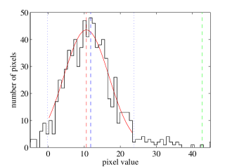
Figure 1: Simulated histogram of pixel values in a background block. The model has a true background of 10mJy with 6mJy Gaussian noise and a single 1Jy source in the centre. The red line is the best fit Gaussian. The fitted peak is is 10.3mJy (red dashed line), the median is 11.3mJy (blue dashed line), and the mean is 42mJy (green dashed line). The dotted blue lines are the $\pm 2\sigma$ from the median.

This technique is valid only so long as the angular scale of a point source is significantly smaller than the scale of background variations. Since we have set the background blocks to be ten times the FWHM of the PSF, this is a good approximation, and the fitted peak of the histogram is very insensitive to bright sources in the block. As a simple test we made a set of 1000 realisations of a model with a background of 10mJy with Gaussian random noise with an rms of 6mJy, and put a single 1Jy Gaussian source in the middle. The resulting histogram for a single realisation is shown in Figure 1. The mean of the block is 42mJy, and so would give an error of 32 mJy if it were used as the background estimate. The median is more robust, leading to an error of 1mJy, and the peak fit is biased by only 0.3 mJy. It is worth noting that background subtraction using simple filtering methods, such as the Mexican Hat filter, are intrinsically linear, and so are approximately equivalent to using the local mean value as the background estimate. This means that they are significantly biased around bright sources.

The background at each pixel is then estimated using a bi-cubic interpolation between the coarse grid of backgrounds, and subtracted from the data. This approach to background estimation is similar to the nebuliser algorithm, developed by the Cambridge Astronomical Survey Unit. After the initial analysis of the science-verification data for the H-ATLAS survey (Rigby et al. 2011), we used nebuliser to perform the background subtraction rather than the inbuilt background subtraction (Valiante et al. 2016, Maddox et al. 2018). This choice was largely based on the much faster run-time of nebuliser compared to the MADX version. The catalogues described in his paper use the built-in MADX background subtraction.

3 Filtering

Typically image data is sampled finely enough that point sources have 2 or 3 pixels within the FWHM in each direction. This means that the flux from a source is spread over many pixels, and the optimal estimate of the source flux is given by a weighted sum over pixels. For an isolated source on a uniform background with uniform Gaussian errors, the minimum variance estimate of the source flux is given by the sum of the data weighted by the point spread function (PSF) at the true position of the source. Cross-correlating the data by the PSF gives the PSF-weighted sum at the position of each pixel, and choosing the peak in the filtered map gives the minimum variance estimate of the source position and source flux (see e.g. Stetson 1987).

If the pixel uncertainties vary spatially, the optimal weighting must also include the inverse of the estimated variance, as derived by Serjeant et al. (2003). If the power spectrum of the noise is not flat, the optimal filter is different from the PSF. In particular, when the source density is high, confusion noise is important, and the optimal filter is narrower than the PSF. The optimal filter, $Q$, can be estimated using a matched filter approach that includes confusion noise (Chapin et al. 2011). In this case, the noise-weighted filtered map, $F$, is given by

$$F=\frac{(DW)\otimes Q}{W\otimes PQ},$$ (1)

where $D$ is the background subtracted data in each pixel, the weight $W=1/\mathrm{var}(D)$ is the inverse of the variance of each pixel, $P$ is the PSF, and $\otimes$ represents the cross-correlation operator. Assuming that the instrumental noise on each pixel in the unfiltered map is uncorrelated, the variance of each pixel in the filtered map is given by

$$V=\frac{W\otimes Q^{2}}{(W\otimes PQ)^{2}},$$ (2)

This is the generalisation of the PSF-filtering approach derived by Serjeant et al. (2003); setting $Q=P$ yields exactly the Serjeant et al. results. The noise-weighting in this step is particularly important for the H-ATLAS data, since the noise varies dramatically on small angular scales depending on the number of detector passes a particular sky position has (Maddox et al. 2018).

The filtered map gives the minimum variance estimate of the flux that a source would have at any given pixel in the map. Standard FFT routines allow easy calculation of the filtered maps at integer pixel positions, but in practice, sources are not centred on pixels. In order to find the best flux estimates, we need to allow for sub-pixel positioning. Without this, the fluxes will be significantly underestimated, particularly when a source lies at the edge of a pixel. Our approach to solving this problem is discussed in Section 5.2.

4 Combining Wavebands

The filtered map in a single band provides an estimate of source flux and uncertainty at any position, and this approach can be extended to include any other wavebands that are available. If we know the observed spectral energy distribution (SED), of a source, $S(\lambda)$, then the flux in a band with response $R(\lambda)$, is given by

$$F=\frac{\int S(\lambda)R(\lambda)d\lambda}{\int R(\lambda)d\lambda},$$ (3)

where we assume the detector measures total energy, as in a bolometer, not the total count of photons as in a CCD. We define the normalised SED as $S_{0}(\lambda)$ where

$$S_{0}(\lambda)=\frac{S(\lambda)}{\int S(\lambda)d\lambda},$$ (4)

so the observed SED of the source is $AS_{0}(\lambda)$, where $A=\int S(\lambda)d\lambda$. Given a set of filter pass-bands, $R_{k}$ and the source SED, the true broad-band flux in each band is $F_{k}=AF_{k0}$, where

$$F_{k0}=\frac{\int S_{0}(\lambda)R_{k}(\lambda)d\lambda}{\int(R_{k}(\lambda)d\lambda}.$$ (5)

Since the value of $A$ does not depend on wavelength, the filtered map in each band gives an independent estimate of $A$. In order to combine the maps, we need to have the estimates at exactly the same position. As discussed in Section 5.2, it is reasonable to use a bi-cubic interpolation to estimate the source flux at non-integer pixel positions. If we interpolate the lower resolution maps to the pixel centres of the highest resolution map, then we can take the inverse variance weighted sum to obtain the minimum variance estimate of $A$ at the pixel positions of the highest resolution map. For waveband $k$ the estimate of $A$ at position $x$ is $A_{k}=F_{k}(x)/F_{k0}$, and the variance is $\sigma_{A,k}^{2}=V_{k}(x)/F_{k0}^{2}$. Hence the overall minimum variance estimate of $A_{\mathrm{tot}}$ is given by

$$A_{\mathrm{tot}}=\frac{\sum_{k}{F_{k}\frac{F_{k0}}{V_{k}}}}{\sum_{k}{\frac{F_{k0}^{2}}{V_{k}}}},$$ (6)

and the uncertainty on $A_{\mathrm{tot}}$ is given by

$$\sigma_{A}^{2}=\frac{1}{\sum_{k}{\frac{F_{k0}^{2}}{V_{k}}}}.$$ (7)

So, the significance of a source detection at any position is $A_{\mathrm{tot}}/\sigma_{A}$. This is a very simple derivation of the standard result first presented by Naselsky, Novikov and Silk (2002). As for the case of a filtered map in a single band, we estimate the most likely position of the source as the position of the peak in the combined significance map.

Note that these formulae include a factor $F_{k0}^{2}$ as part of the weight given to the waveband $k$, so that the true SED acts as a weighting term for each band as well as the inverse variance factor. This makes intuitive sense: if a source’s flux is expected to peak in a particular band, we should give that band the most weight in determining the position of the source; if a source has a flat spectrum, so that the flux is equal in all bands, then all bands are given equal weight. In general we do not actually know the true SED of any particular source, and clearly don’t know the SED of sources that we have not yet detected. However, we can maximise the detection rate of a particular type of source by choosing an SED prior to match.

This derivation considers an isolated source, but we can filter and combine the full area of available data to produce a global significance map, and find all the peaks to consider as potential sources. For H-ATLAS, we kept those that are more than $2.5\sigma$ as potential sources. In principle we could retain all peaks, but rejecting the low-significance peaks gives a large saving in computing time, while not losing any significant detections.

5 Source parameters

5.1 Estimating positions and fluxes

To estimate the position of each source, we perform a variance weighted least-squares fit of a Gaussian to the $5\times 5$ pixels around each peak. The position of the peak is allowed to vary freely, and is not constrained to be at integer pixel positions. We fit only to pixels near the peak to minimise the effects of confusion from other nearby sources. Since the individual maps have been filtered, the peak pixels already include data from the surrounding raw pixels, combined in an optimal way; the peak fitting is solely to find the position at the sub-pixel level.

In order to estimate the flux in each band, we use the individual filtered maps, and interpolate to find the value of each map at the position of the peak in the combined map. For an isolated source, this will provide the optimal flux estimates. However, if there are sources that are close together, so that the PSFs significantly overlap, this simple approach will ‘double-count’ flux, because the wings of each source add on to the peak of its neighbour. A simple way to avoid this problem is to sort the sources in order of decreasing flux based on their initial peak-pixel value, and then estimate the optimal fluxes in sequence. After getting the optimal fluxes for a source, we subtract the scaled filtered PSF from the maps before estimating the fluxes for the next source. This is similar in concept to the clean algorithm (Högbom 1974) but with just one pass. This process is done separately for each band, so the ‘clean’ works from the brightest sources in each band. In principle, the procedure could be iterated to a stable solution, but in practice the difficult cases are blends of sources that require a more sophisticated de-blending technique to improve the flux estimates. So iterating this simple clean algorithm would provide a very small gain in reliability at a large computational cost.

To provide the uncertainty for each flux measurement, we create a map of the filtered noise, using equation 2 and perform the same interpolation to estimate the flux variance in each band at each source position.

5.2 Sub-pixel subtleties

The above analysis ignores the complication that our data typically sample the sky with only 2 or 3 pixels across the FWHM of the PSF. When the PSF is sampled into coarse pixels, the value of the peak pixel is averaged over the whole area of the central pixel, and so is suppressed relative to the peak of the true PSF. For a PSF that is close to a Gaussian with 3 pixels across the FWHM, this suppression is typically $\sim 5$ per cent. Since we use the pixelated PSF (the Point Response Function - or PRF) when filtering the data, the filtered data is boosted by the suppression factor, and so the estimated flux for source that is centred in a pixel is unbiased. For a source that is not centred in a pixel, the observed peak value is suppressed compared to a pixel centred source.

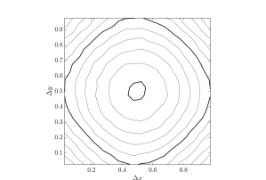
Figure 2: Mean fractional flux errors as a function of the precise source position within a pixel. The contours are linearly space from 0 to $-0.9$ per cent. The central thicker contour corresponds to mean error of 0, and the outer thicker contour is $-0.5$ per cent. The maximum error is $\sim-1$ per cent for a source in the corner of 4 pixels.

In order to obtain the most accurate estimates of source flux for an arbitrary position, we need to consider the true flux distribution within the footprint of each pixel. An obvious way to improve on the flux estimated from individual pixel values is to interpolate between them. However, a bi-linear interpolation does not remove the bias, as can be seen by considering a source that is exactly half way between two pixels; each pixel will have the same value that is less than the true peak value, so the interpolated value will also be biased low. A bi-cubic interpolation allows the interpolated value to be higher than either individual pixel, and so gives a better flux estimate.

Since we estimate the source positions by fitting a Gaussian to the central $5\times 5$ pixels of each source, the positions are not directly affected by the pixelization; for signal to noise ratio greater than 20 we find that the source positions are accurate to better than 1/12 of a pixel (see Figure 7). So, to estimate the flux of the source, we use the filtered maps interpolated to the best fit sub-pixel position. If the source position lies at the centre of a pixel, the interpolation returns that pixel value, and this will be an unbiased flux estimate. If the source position lies at the boundary between two pixels, the pixel values are suppressed relative to the peak of the pixel-centred PSF, but the bi-cubic interpolation means that the estimated flux will be higher than the pixel values, thus reducing the suppression. We tested this effect by creating simulated data at higher resolution, averaging over the small pixels to produce a low-resolution data, and then measuring the recovered flux from the interpolated, filtered low-resolution data. We find the interpolation reduces the suppression due to pixelization, but does leave a slight underestimate of the actual peak. The fractional flux error as a function of position is shown in Figure 2. The error is zero at the centre of a pixel, and smoothly increases towards the pixel edges. It is largest for a source at the corner of 4 pixels when the flux is underestimated by $\sim 1$ per cent. Although the simulations are specific to a simple Gaussian PSF, this is a good approximation to the H-ATLAS data. In fact, the PSF in most astronomical data can be approximated by a Gaussian near the peak, and the pixel scales are typically chosen to sample the FWHM at a similar spacing, and so similar improvements are likely for other data.

6 Tests of the methods

6.1 Simulations

As a simple test of the source detection algorithm we generated maps covering $3.4^{\circ}\times 13.6^{\circ}$, in three bands: 250, 350 and 500 $\mu$m . This is equivalent to a single one of the three H-ATLAS equatorial fields (Valiante et al. 2016). Sources are placed on a grid of positions separated by 3 arcminutes on the sky with a small blank area around the edges of the maps, leading to 17750 sources in the maps. Each source is assigned a small random offsets from the exact grid centre, so that the pixels sample the PSF with random offsets from the pixel centres. The PSF for each band is chosen to be a Gaussian with full-width half maximum of 18, 24 and 36 arc seconds respectively, roughly matching the Herschel beam in the three bands. The PSF is over-sampled by a factor of 50, (corresponding to 0.12 arc-second pixels in the 250 $\mu$m band) and re-binned to the final pixel sizes of 6, 8 and 12 arc seconds, chosen to match the H-ATLAS maps. Each source is given a 250 $\mu$m flux between 1mJy and 1Jy, uniformly spaced in log flux. This is clearly not a good match to the flux distribution of real sources, but is a simple way to provide good statistics over the full flux range. The 350 $\mu$m and 500 $\mu$m fluxes for each source are then assigned so that the SED matches a modified black body with $\beta$ chosen from a uniform random distribution between 1 and 2, and temperature, $T$, randomly chosen from a log-normal distribution centred on $T=25$K, and ranging from 20K to 35K, as shown in Figure 3. This distribution roughly matches the SEDs of low-redshift galaxies seen in the H-ATLAS survey (Smith et al. 2012).

Sources are included following a two-component redshift distribution with a low-redshift population peaking at $z=0.3$, and a high redshift population extending to $z\sim 2$ with a peak at $z=1.2$. This reproduces the $F_{250}/F_{350}$ colour distribution observed in the H-ATLAS survey, as shown in Figure 4. Although these simulations provide a reasonable match to the $F_{250}/F_{350}$ colour of real data, they are not red enough in the $F_{500}/F_{350}$ colour distribution. To investigate the impact for redder sources, we also considered simulations with an extended tail of high redshift sources which leads to an enhanced population of extremely red sources (Ivison et al. 2016). Finding a best fit model which reproduces the observed colour distributions is beyond the scope of this paper, but the real H-ATLAS data will be somewhere between these two sets of simulations.

Figure 3: The temperature distribution of simulated sources. The red line shows the scaled and shifted log-normal probability distribution used to generate the temperatures. The blue histogram shows the source counts for a single realisation of the simulations.

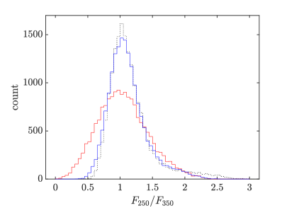
Figure 4: The $F_{250}/F_{350}$ colour distribution of simulated sources compared to that observed in the H-ATLAS survey. The black dotted histogram shows the observed colour distribution. The blue histogram shows the distribution for a particular realisation with matching colour distribution. The Red histogram shows a simulation with a extended high-z population .

We also added a galactic background by taking the 100 $\mu$m and temperature maps from Schlegel, Finkbeiner and Davis (1998) and scaling the 100 $\mu$m emission to the relevant wavelength using a modified black-body. The resolution of these maps is several arcminutes, and so does not contain small-scale structure in the cirrus background. The HATLAS data show that in some patches of sky there is strong cirrus emission with significant structure on sub-arc-minute scales, but in most areas, the emission is relatively smooth. Our simulated background is a reasonable approximation for most of the sky, but will be somewhat easier to subtract than the areas where the true cirrus is particularly strong and structured.

Finally we add Gaussian noise to the maps. The standard deviation is set to roughly match the instrumental noise in the H-ATLAS survey (Valiante et al. 2016). The values we use here are 9.3, 9.8 and 13.5 mJy per pixel in the 250, 350 and 500 $\mu$m bands respectively. Note that the sources are positioned on a grid, and so do not suffer from confusion noise, meaning that the appropriate matched filter is the PSF. We consider confusion noise and the modified matched filter in Section 6.3

We then run MADX on the simulated maps to detect the sources and measure their position and fluxes. We used several different priors: first using only the single bands for the detection: weights 1,0,0 for the 250 $\mu$m band; weights 0,1,0 for the 350 $\mu$m band; weights 0,0,1 for the 500 $\mu$m band. Second, we used equal weighting for each band (weights 1,1,1), corresponding to a flat spectrum source. By design, the sources are on a grid, and cannot overlap, so a simple positional match allows us to associate the detected sources to the corresponding input sources, and calculate the errors in position and fluxes. We identify a recovered source with an input source if the recovered position is within one pixel of the input position. For very low signal-to-noise detections, the large standard deviation of the positional errors means that some detections are not matched within the one pixel radius. This has a small effect on the catalogue completeness, but the dominant source of incompleteness is simply noise on the flux estimates.

6.2 Results

(a)
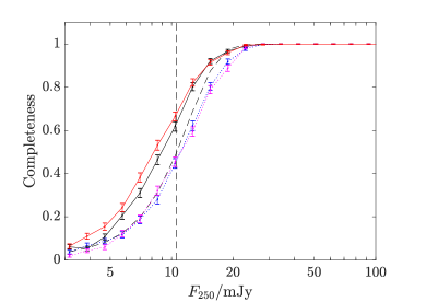
(b)
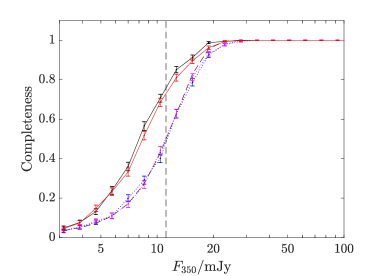
(c)

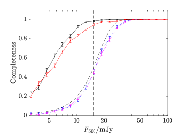
Figure 5: Completeness of recovered source catalogues as a function of flux in each band. The blue and black lines are for simulations which match the H-ATLAS colour distribution; the red and magenta include a high-redshift red population. The dotted lines are for source detection using only the relevant single band in each panel, and the solid lines are for detection using the equal weighting of bands. The dashed curves show the expected completeness from Gaussian errors and the vertical dashed lines show the 2.5-$\sigma$ detection threshold. In the 250 $\mu$m band, using the flat prior pushes the 50 per cent completeness limit about a factor 1.25 deeper. In the 350 $\mu$m and 500 $\mu$m bands the gains using the flat prior are factors of 1.28 and 3 for the colour-matched simulations. The effect of the red population is to slightly reduce the completeness in the 350 and 500 $\mu$m bands. This is a small effect as a percentage of the full catalogue, but represents a significant improvement for the red population itself.

(a)
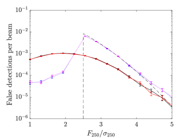
(b)
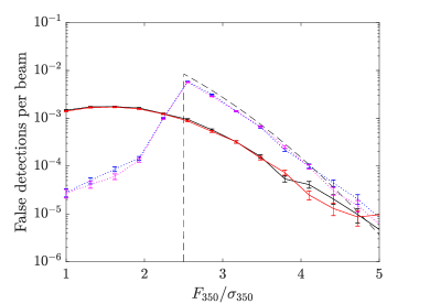
(c)

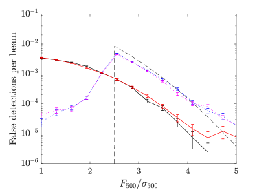
Figure 6: The number of false detections per beam as a function of signal to noise. The blue and black lines are for simulations which match the H-ATLAS colour distribution; the red and magenta include a high-redshift red population. The dotted lines are for source detection using only the relevant single band and the solid lines show the equal weighting of bands. The dashed lines show the expected rate of false detections from Gaussian errors and the 2.5-$\sigma$ threshold applied during the MADX detection. For the 250 $\mu$m and 350 $\mu$m bands, the flat prior reduces the false detection rate by about a factor 4 at the 4-$\sigma$ limit, and a factor 6 at 3-$\sigma$. In the 500 $\mu$m band the gain is roughly a factor 10 between 2 and 4-$\sigma$. The inclusion of the extra red population does not significantly change the false detection rates.

For each simulation, we measure the completeness by simply counting the fraction of input sources that are detected as a function of flux. Figure 5 shows the completeness as a function of flux in each band for both the colour-matched and red-population simulations, and for catalogues using the single-band priors and the flat priors. The blue lines are for colour matched simulations with catalogues using the single band prior and the black lines use the flat prior. It is clear that including information from all three bands significantly improves the completeness of the resulting catalogue. The flux limit at 50 per cent completeness in the 250 $\mu$m and 350 $\mu$m band samples is a factor $\sim 1.4$ deeper using the multi-band approach compared to the single band method. The gain for the 500 $\mu$m band is about a factor of 3, reflecting the very large gain in signal to noise ratio by using the information from the other bands to identify sources. The improvements are very similar for the simulations with extra red sources.

The noise in the maps leads to peaks that are detected as a source, but do not correspond to an input source. The number of false detections per beam area is shown as a function of signal to noise for each band in Figure 6. Using the flat-prior detection reduces the number by a factor between 4 and 10 in all bands compared to the single-band detection. Including extra red sources in the simulations makes no significant difference to the rate of false detections. For the single band detections, the expected number of noise peaks for Gaussian noise with a 2.5-$\sigma$ cut is shown by the dashed line. The observed number of false detections follows this very well above the 2.5-$\sigma$ cut. There are a small number of sources with fluxes below the 2.5-$\sigma$ limit, and this is because cut is applied to the initial peak pixel value, while the final flux plotted on $x$-axis uses the flux measured at the interpolated peak position. The noise between the two flux estimates scatters some sources below the initial cut. In practise for the real H-ATLAS data we apply a much higher limit (between 4 and 5$\sigma$) in the final catalogue, so this effect is not visible.

(a)
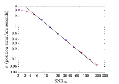
(b)

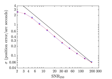
Figure 7: The measured positional errors of simulated sources plotted as a function of signal-to-noise in the 250 $\mu$m band. The standard deviation of the errors in RA are shown as blue circles, and in Dec shown as red crosses. Panel (a) shows the measurements using only the 250 $\mu$m band to detect sources and measure their positions. Panel (b) shows the measurements using the flat-prior detection. The black line in both panels shows the variation expected from the theoretical analysis of Ivison et al. (2007). For signal-to-noise ratio less than four the 1 pixel matching criterion means that some true matches with large positional errors have not been included in the matched sample, and this reduces the apparent $\sigma$. A 2-d Gaussian with $\sigma=4$ truncated at 1 pixel radius ($=6^{\prime\prime}$) has a standard deviation of $2.7^{\prime\prime}$, as we see here.

Next we compare the measured positions to the input positions. While including data from lower resolution, or lower signal-to-noise bands could increase the positional errors, extra information is provided by summing data with the correct weighting, and the positional accuracy is improved. This can be seen in Figure 7, which shows the rms position error in RA and Dec as a function of signal-to-noise, defined as $A_{tot}/\sigma_{A}$ from equations 6 and 7. Using only the 250 $\mu$m band to detect the sources leads to positional errors in good agreement with the theoretical expectations from Ivison et al. (2007). Including all bands significantly reduces the positional errors, even though the other bands have poorer resolution. At low signal-to-noise (SNR$\mathrel{\hbox{\hbox to0.0pt{\hbox{\lower 4.0pt\hbox{$\sim$}}\hss}\hbox{$<$}}}4$) the apparent positional error starts to flatten because only the sources within one pixel are counted as matches, and the apparent standard deviation is biased too low.

Finally we compare the measured and input fluxes for the sources, in terms of both random and systematic errors. To assess the random errors, we simply calculate the standard deviation of the between the difference between the measured and input fluxes. Over the range of interest, we find that this does not vary significantly as a function of flux, and is 4.4, 4.6 and 6.4 mJy for the 250 $\mu$m , 350 $\mu$m and 500 $\mu$m bands respectively. These are between 3 and 6 per cent higher than the values of 4.2, 4.5 and 6.1 mJy expected from the simple application of equation 2 the estimate the flux errors. This small discrepancy is likely to be caused by sub-pixel positioning effects and residual background subtraction errors. The choice of prior makes no significant difference to the flux errors, as these errors are dominated by the pixel-to-pixel flux errors on the map for each band. Also the colour distribution used in the simulations makes no significant difference to the errors.

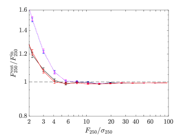
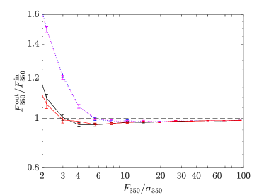
(a) (b) (c)

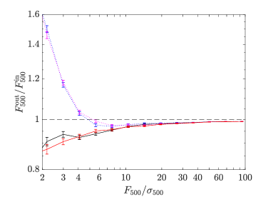
Figure 8: The ratio of mean measured flux compared to the mean input flux as a function of input signal to noise for different source detection priors. The blue lines show the single-band priors, and the black lines use a flat prior. Panels (a),(b) and (c) shows the results for the 250 $\mu$m , 350 $\mu$m and 500 $\mu$m fluxes respectively. Using the single-band source detection leads to significant flux boosting in the measured fluxes. For the 250 $\mu$m and 350 $\mu$m bands, the flat prior reduces the boosting effect at fainter fluxes. For the 500 $\mu$m band, the flat-prior fluxes are systematically underestimated at fainter fluxes. The red and magenta lines show the results from simulations with extra red sources. The red sources do not introduce any significant changes.

Figure 8(a) shows the mean ratio of measured to input flux as a function of signal to noise. At high signal to noise there is a small ($\sim$0.5 per cent) underestimate of flux due the peak pixelization issues discussed in Section 5.2. For sources with fluxes near the detection limit, there is a systematic bias to higher fluxes when using the single-bands to detect sources (flux boosting). This is related to Eddington/Malmquist bias when selecting sources to be above a signal-to-noise threshold: faint sources with negative errors are not retained in the catalogue, whereas those with positive errors are detected to a fainter level. The precise form of the boosting depends on the distribution of true source fluxes, as well as the measurement errors. For our current simulations we chose to distribute sources uniformly in log flux, and so they do not match real source flux distributions, even though the colours are realistic. Hence we cannot use them to estimate the boosting as a function of flux for real data. Valiante et al. (2016) created realistic simulations and used them to estimate both the completeness and boosting correction factors that apply to the H-ATLAS data.

Using the flat prior combination to detect sources includes information from all three bands, and so reduces the bias from noise peaks in any single band, leading to significantly reduced flux boosting. For the 500 $\mu$m band, the angular size of the PSF is larger, and the signal-to-noise is significantly smaller than the other two bands. This mean that it contributes only a small amount to the detection signal and positional measurement. The positional errors mean that the local peak is missed and the flux estimate is systematically underestimated. This bias can be corrected using the average values measured from simulations (Valiante et al. 2016).

The flux boosting and biases are not significantly affected by the inclusion of extra red sources in the simulations.

6.3 Confusion Noise

The simulations described so far contain no confusion noise, and so the appropriate optimal filter is simply the PSF. To test the performance of the modified matched filter approach, we have added confusion noise to each pixel in the simulations as an extra term consisting of PSF-filtered Gaussian noise, with the variance as seen in the H-ATLAS data (Valiante et al. 2016). The corresponding standard deviation is $\sim$7 mJy per pixel in all three bands. We use these values of confusion noise to calculate the matched filters as described in Appendix A of Chapin et al. (2011). We then re-ran the image detection based on the single-band priors, and used both the PSF filter and the matched filter. We also used the flat-prior detection with the matched filters. The resulting completeness comparisons are shown in Figure 9. The matched filter selection improves the completeness at a given signal to noise cut, providing a catalogue $\sim$20 per cent deeper. As before, using the flat prior detection also provides an improvement of a factor $\sim 1.3$ in flux at the same completeness level for the 250 $\mu$m and 350 $\mu$m bands, and a factor 2 for the 500 $\mu$m band. Overall the two modifications give a catalogue that is a factor of 1.5 to 3 deeper in flux at 50 per cent completeness.

The added confusion noise means that the flux errors are larger than for the simulations with only Gaussian noise. Using the matched filter reduces the errors by about 10 per cent compared to using the PSF. As an aside, we note that using the matched filter for the Gaussian noise simulations leads to a 14 per cent increase in flux errors compared to the PSF filter. This is exactly as would be expected since the optimal filter for data with Gaussian noise is the PSF, and the optimal filter for data with confusion noise is the appropriate matched filter.

As shown in Figure 10, using the matched filter reduces the number of false detections by a factor 8 at the 4-$\sigma$ limit for the 250 $\mu$m band. Using the flat prior as well reduces the rate by a further factor 2. In the 350 $\mu$m and 500 $\mu$m bands the matched filter provides similar reductions in the false detection rate.

Figure 11 shows the ratio of measured to input fluxc when confusion noise is included. The behaviour is very similar to that shown in Figure 8 for simple Gaussian noise. At high signal to noise there is a small ($\sim$0.5 per cent) underestimate of flux due the peak pixelization issues discussed in Section 5.2. Near the detection limit, the single-band detection leads to significant flux boosting. Using the flat prior to detect sources reduces this effect. For the 500 $\mu$m band, the positional errors again mean that the fluxes are underestimated, but the effect is slightly smaller than for Gaussian noise because the confusion noise has less power on the small scales that directly affect the position estimates.

7 Summary

We have presented a simple approach to detecting sources in data which consists of multiple broad-band images. For high signal to noise sources, fitting a Gaussian to estimate the source position and using bi-cubic interpolation to estimate fluxes significantly improves the accuracy over single pixels estimates. Combining multiple bands in an optimal way before detecting images leads to a significant improvement in sensitivity to faint sources, a reduction in the number of false detections, and an improvement in positional accuracy. Using a matched filter which accounts for confusion noise improves the signal-to-noise ratio of individual flux measurements and so further improves the source detection reliability. Together the two modifications provide catalogues a factor two to three deeper than possible with a standard single-band PSF filter approach.

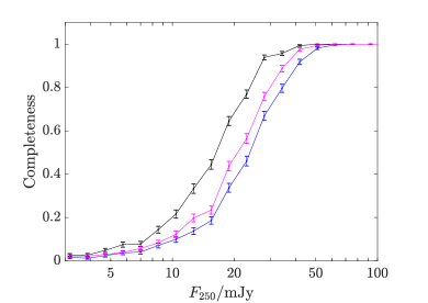
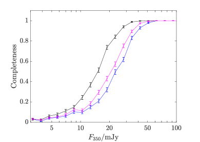
(a) (b) (c)

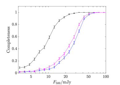
Figure 9: Completeness of recovered source catalogue as a function of flux in each band for simulations with confusion noise included. The blue lines are for source detection using the appropriate single-band prior and PSF filtering; the magenta lines are for source detection using the single-band priors, but with the matched filters; and the black lines use the matched filters and equal weighting of bands.

(a)
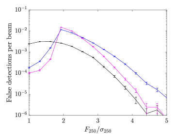
(b)
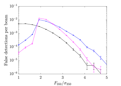
(c)

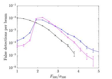
Figure 10: The number of false detections per beam as a function of signal to noise for simulations with confusion noise. The blue lines are for source detection using the appropriate single-band priors and PSF filtering; the magenta lines are for source detection using the single-band priors, but with the matched filters; and the black lines use the matched filters and the equal weighting of bands. In the 250 $\mu$m band, using the matched filter reduces the false detection rate by a factor 8 at the 4-$\sigma$ limit. Using the flat prior source detection reduces it by a further factor of 3. In the 350 and 500 $\mu$m bands the gain is roughly a factor 10 between 2 and 4-$\sigma$.

(a)
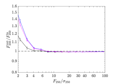
(b)
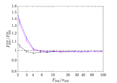
(c)

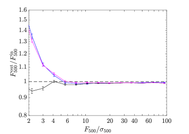
Figure 11: The ratio of mean measured flux compared to the mean input flux as a function of input signal to noise for different source detection priors for simulations with confusion noise included. The blue lines show the single-band priors with a PSF filter; the magenta lines show the single-band priors with a matched filter; the black lines show the flat prior with a matched filter. Panels (a), (b) and (c) shows the results for the 250 $\mu$m , 350 $\mu$m and 500 $\mu$m fluxes respectively. Using the single-band source detection leads to significant flux boosting in the measured fluxes. The flat prior reduces the boosting effect at fainter fluxes.

References

- Amvrosiadis et al. (2019) Amvrosiadis, A., et al. 2019, MNRAS, 483, 4649
- Bertin (1996) Bertin, E., 1996, AAPS, 117, 393
- Chapin et al. (2011) Chapin, E. L. et al. 2011, MNRAS, 411, 505
- Eales et al. (2010) Eales, S., et al. 2010, PASP, 122, 499
- González-Nuevo et al. (2006) González-Nuevo et al. 2006 MNRAS, 369, 1603
- Grumitt et al. (2020) Grumitt et al. 2020 arXiv:1910.08583v1
- Herranz et al. (2002) Herranz et al. 2002 MNRAS, 336, 1057
- D. Herranz et al. (2005) Herranz, D., et al., MNRAS, 356, 944
- Herranz, Argüeso and Carvalho (2012) Herranz, Argüeso and Carvalho 2012, Advances in Astronomy, 2012 id. 410965
- Högbom (1974) Högbom, J.A., 1974, ApJSup, 15, 417
- Irwin (1985) Irwin, M.J. 1985, MNRAS, 214, 575
- Ivison et al. (2016) Ivison, R.J., et al. 2016, ApJ, 832, 78.
- Ivison et al. (2007) Ivison, R. J., et al. 2007, MNRAS, 380, 199
- Kay (1998) Kay, S.M, 1998, Fundamentals of Statistical Signal Processing: Detection Theory, (Prentice-Hall, London).
- Lanz et al. (2010) Lanz et al. 2010 MNRAS, 403, 2120
- Maddox et al. (2010) Maddox, S. J., Dunne, L., Rigby, E., et al. 2010, A&A, 518, 11.
- Maddox et al. (2018) Maddox, S. J., Valiante, E., Cigan, P., et al, 2018, ApJSup, 236, 30.
- Naselsky, Novikov and Silk (2002) Naselsky, P., Novikov, D. and Silk, J., 2002, MNRAS, 335, 550
- North (1943) North, D. O., 1943, Proc IRE 51, 1016-1028 (rep. July 1963)
- Pilbratt et al. (2010) Pilbratt, G. et al., 2010, A&A, 518. 1.
- Planck Collaboration Int. LIV. (2018) Planck Collaboration Int. LIV. 2018, A&A, 619, A94
- Pratt (1978) Pratt, W.K, 1978 Digital Image Processing, Wiley.
- Rigby et al. (2011) Rigby et al, 2011, MNRAS, 415, 2336.
- Schlegel, Finkbeiner and Davis (1998) Schlegel, Finkbeiner and Davis, 1998, ApJ, 500, 525.
- Serjeant et al. (2003) Serjeant et al. 2003, MNRAS, 344, 887.
- Smith et al. (2012) Smith, D. J. B., et al., 2012, MNRAS, 427, 703.
- Stetson (1987) Stetson 1987, PASP, 99, 191.
- Tegmark & de Oliveira-Costa (1998) Tegmark & de Oliveira-Costa 1998, ApJ, 500, 83
- Valiante et al. (2016) Valiante, E., et al., 2016, MNRAS, 462, 3146
- Vielva et al. (2003) Vielva et al., 2003 MNRAS, 344, 89
(a) (b)
(b) (c)
(c)
(a)
(b)
(c)
(a)
(b)
(c)