Model-based Joint Bit Allocation between Geometry and Color for Video-based 3D Point Cloud Compression

Abstract

Rate distortion optimization plays a very important role in image/video coding. But for 3D point cloud, this problem has not been investigated. In this paper, the rate and distortion characteristics of 3D point cloud are investigated in detail, and a typical and challenging rate distortion optimization problem is solved for 3D point cloud. Specifically, since the quality of the reconstructed 3D point cloud depends on both the geometry and color distortions, we first propose analytical rate and distortion models for the geometry and color information in video-based 3D point cloud compression platform, and then solve the joint bit allocation problem for geometry and color based on the derived models. To maximize the reconstructed quality of 3D point cloud, the bit allocation problem is formulated as a constrained optimization problem and solved by an interior point method. Experimental results show that the rate-distortion performance of the proposed solution is close to that obtained with exhaustive search but at only 0.68% of its time complexity. Moreover, the proposed rate and distortion models can also be used for the other rate-distortion optimization problems (such as prediction mode decision) and rate control technologies for 3D point cloud coding in the future.

I Introduction

With the rapid development of 3D scanning techniques [1], point clouds are now readily available and popular [2]. There are already many 3D point cloud applications in the fields of 3D modeling [3] [4], automatic driving [5], 3D printing [6], augmented reality [7], etc. Compared with traditional 2D images and videos, a 3D point cloud describes the 3D scene or object with the geometry information and the corresponding attributes (e.g., color, reflectance) [8]. To represent a 3D scene accurately, millions of points must be captured and processed. This huge data volume poses a severe challenge for efficient storage and transmission. In the past few years, major progress in both static and dynamic point cloud compression has been made [9]. To compress the 3D point cloud (especially the attribute information) effectively, transforms that can adapt to the irregular structure of the 3D point cloud were exploited. These include the shape-adaptive discrete cosine transform [10], graph transforms [11] [12] [13], region-adaptive hierarchical transforms [14, 15, 16, 17], Gaussian process transforms [18] [19], and sparse representation based on virtual adaptive sampling [20] [21]. Based on the previously mentioned graph transforms, Shao et al. [22] further combined a slice partition scheme and an intra prediction technique to improve the performance of attribute compression. Instead of compressing the irregular data directly, some researchers [23] [24] try to map the irregular data to a regular representation (e.g., a 2D plane) to simplify the task. Similar ideas were previously proposed to compress 3D human motion [25] and 3D facial expression [26, 27, 28, 29]. All the described methods are mainly designed for static point clouds. Since dynamic point clouds are becoming more and more essential in practical applications, efficient compression methods for dynamic point clouds are also required. Because of the inter-frame redundancy of dynamic point clouds, motion estimation and motion compensation are the key technologies to effectively compress dynamic point clouds. Thanou, Chou and Frossard [30] focused on motion estimation by using a spectral graph wavelet descriptor. De Queiroz and Chou [31] proposed a motion compensation approach to encode dynamic voxelized point clouds. Anis, Chou and Ortega [32] simplified motion compensation by representing sets of frames in a consistently evolving high-resolution subdivisional triangular mesh.

To standardize 3D point cloud compression (PCC) technologies, the Moving Pictures Expert Group (MPEG) launched a call for proposals in 2017. As a result, three point cloud compression technologies were developed: surface point cloud compression (S-PCC) with software platform TMC1 [33] for static point cloud data, video-based point cloud compression (V-PCC) with software platform TMC2 [34] for dynamic content, and LIDAR point cloud compression (L-PCC) with software platform TMC3 [35] for dynamically acquired point clouds. Recently, L-PCC and S-PCC were merged under the name geometry-based point cloud compression (G-PCC) with software platform TMC13 [36].

In this paper, we focus on the V-PCC platform (TMC2) due to its excellent performance for compressing both static and dynamic point clouds. As shown in Fig. 1, the main philosophy behind V-PCC is to leverage state-of-the-art video coders for PCC [37].

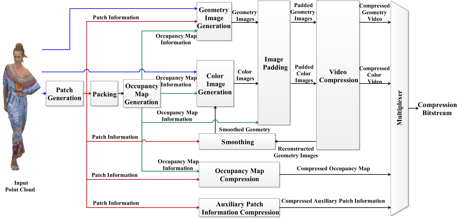
Figure 1: General framework of the V-PCC encoder.

This is essentially achieved by decomposing each point cloud of a sequence of 3D point clouds into a set of patches, which are independently mapped to a 2D grid of uniform blocks. This mapping is then used to store the geometry and color information as one geometry image and one color image. The sequences of geometry images and color images corresponding to the dynamic point cloud are then compressed separately with a video coder, e.g., H.265/HEVC. Finally, the geometry and color videos, together with metadata (occupancy map for the 2D grid, auxiliary patch and block information) are used to reconstruct the dynamic 3D point cloud. Please refer to [38] for more details.

The bitstream of a compressed 3D point cloud consists of two parts: geometry information and color information. For a given platform, the size of each part is controlled by a quantization parameter, which can take a large number of values. At the same time, quantization introduces distortion, which may affect the reconstruction quality. The aim of this paper is to find the pair of quantization parameter values (one for the geometry and one for color) that minimizes the reconstruction error subject to a constraint on the total number of bits. Since the number of candidates is very large, finding an optimal solution with exhaustive search is too time consuming and infeasible in practice as it requires encoding and decoding the point cloud multiple times. In this paper, we address this challenge by proposing analytical models for the rate and distortion and using an interior point method to efficiently solve the rate-distortion optimization problem. The contributions in this paper are as follows.

1. We propose analytical models that characterize the rate and distortion of the geometry and color as functions of the V-PCC quantization steps.

2. We exploit the proposed analytical models to formulate the bit allocation problem for V-PCC as a constrained optimization problem.

3. We use an interior point method to efficiently solve the optimization problem.

Rate distortion optimization plays a very important role in video/image coding. But for 3D point cloud, rate distortion optimization as well as bit allocation/rate control technologies are not investigated before our research. To the best of our knowledge, this is the first time that the rate and distortion characteristics of 3D point cloud are investigated in detail. The proposed rate and distortion models can not only be used for the joint bit allocation of geometry and color but also used for the rate-distortion optimization and rate control technologies for 3D point cloud coding. Based on the derived rate and distortion model, in this paper, we focus on the typical and challenging rate distortion optimization problem, i.e., optimal quantization parameters decision for geometry and color, for 3D point cloud coding. Extensive experimental results demonstrate the advantage and effectiveness of our method. In [8], we used a similar approach for the Point Cloud Library (PCL)-based codec [23] [39]. The PCL-based encoder recursively subdivides the point cloud into eight subsets. This results in an octree data structure, where the position of each voxel is represented by its center whose attribute (color) is set to the average of the attributes of the enclosed points. Then the octree data is encoded by an entropy coder. In order to encode the color attributes, the octree attributes are mapped directly to a structured image grid using depth first tree traversal and then the image grid is encoded with the JPEG codec.

There are three main differences between this paper and our previous work [8].

First, since the two codecs are different, both the rate-distortion analysis and the modeling of the rate and distortion functions are different.

Second, the objective function for the rate-distortion optimization, as well as the optimization variables are different. In this paper, the objective function is the overall distortion, which includes the distortion of both geometry and color information, and the optimization variables are the quantization parameters for the geometry and color information. In [8], only the color distortion is minimized, and the optimization variables are the octree level and the JPEG quality factor.

Third, in contrast to our previous paper [8], where the models are obtained using a simple and rough statistical analysis without theoretical justification, we derived the models theoretically in this paper, and then verified the accuracy of the models by experiments.

The remainder of this paper is organized as follows. In Section II, we formulate the rate-distortion optimization problem for V-PCC and provide analytical models for the distortion and rate as a function of the quantization steps. In Section III, we use these models to solve the rate-distortion optimization problem with an interior point method. In Section IV, we present experimental results where we compare the accuracy of our approach to that of exhaustive search. Section V gives our conclusions and suggests future work.

II Rate and Distortion Models Derivation

To efficiently solve the bit allocation problem, we formulate it as a constrained optimization problem by deriving rate and distortion models for the 3D point cloud. As the distortion of a 3D point cloud is determined by the coding distortion of both geometry and color information, the bit allocation problem can be expressed as

$$\min_{(\emph{$R_{g},R_{c}$})} D(D_{g},D_{c})$$ (1)

$$\mathrm{s.t.} R_{g}+R_{c}\leq\emph{$R_{T}$},$$

where the distortion $D$ of the reconstructed 3D point cloud is determined by the color distortion ($D_{c}$) and the geometry distortion ($D_{g}$); $R_{g}$ and $R_{c}$ are the geometry and color bitrate, respectively, and $R_{T}$ is the target bitrate for both the geometry and color. It is worth noting that the occupancy map and auxiliary information also consume bitrate resources. The occupancy map is a binary array that indicates whether a pixel position is occupied or not. The auxiliary information is just used to store a few encoder parameters. In general, both the occupancy map and the auxiliary information are compressed without loss. In addition, their bitrate cost is small and fixed for a given 3D point cloud. Therefore, we do not consider the bitrate of the occupancy map and auxiliary information in (1). Because both $R_{g}$ and $R_{c}$ are controlled by the quantization parameters (QPs) of the color and geometry coders, the problem is to find the values of the corresponding quantization steps $Q_{g}$ and $Q_{c}$ to achieve optimal quality under a given target bitrate. In the next section, we develop distortion and rate models with respect to the quantization steps, so that the bit allocation problem (1) can be solved analytically.

II-A Distortion Model

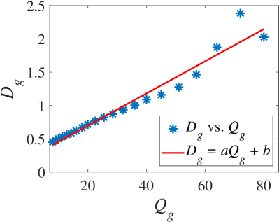
Figure 2: Illustration of the relationship between the geometry distortion $D_{g}$ and the geometry quantization step $Q_{g}$. (a) Phil, (b) Longdress, (c) David, (d) Loot.

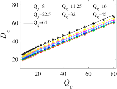
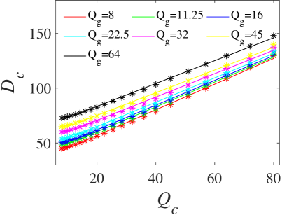
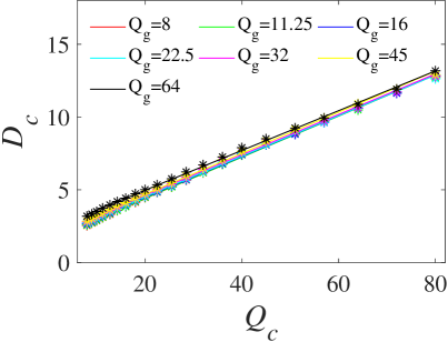
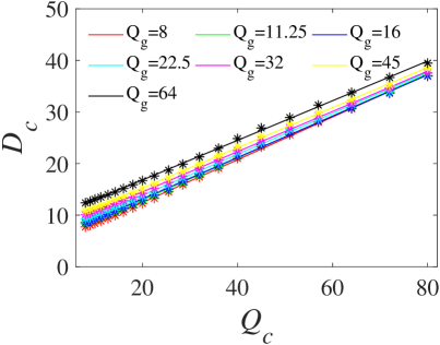
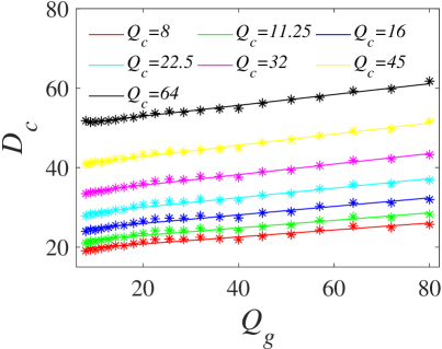
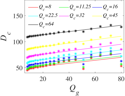
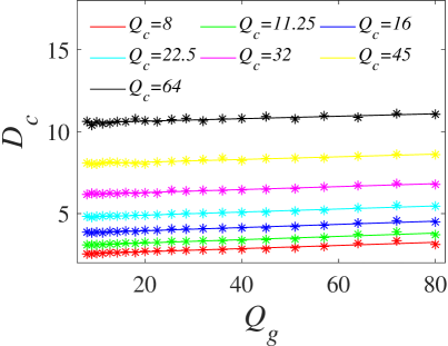
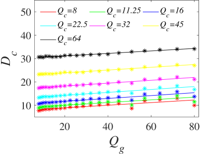
Figure 3: Statistical results for $f_{g}(Q_{g})=\alpha_{gc}Q_{g}+\beta_{gc}$ and $f_{c}(Q_{c})=\alpha_{cc}Q_{c}+\beta_{cc}$. (a)-(d): relationship between $D_{c}$ and $Q_{c}$ for Phil, Longdress, David, and Loot, (e)-(f): relationship between $D_{c}$ and $Q_{g}$ for Phil, Longdress, David, and Loot.

The mean squared error (MSE) is widely used as the distortion metric for point clouds. We calculate it as a linear combination of the geometry distortion and color distortion. That is,

$$D=\omega D_{g}+\left(1-\omega\right)D_{c},$$ (2)

where $D_{g}$ is the geometry distortion, $D_{c}$ is the color distortion, and $\omega$ is a weighting factor. In this paper, we use the symmetric point-to-point distortion defined as follows  [40]. Let A and B denote the original point cloud and the reconstructed point cloud, respectively. Then $D_{g}=max(e^{B,A}_{g},e^{A,B}_{g})$. Here, for two point clouds $A$ and $B$,

$$e^{B,A}_{g}=\frac{1}{|B|}\sum_{b_{i}\in B}\|b_{i}n_{A}(b_{i})\|^{2}_{2},$$ (3)

where $|B|$ denotes the number of points in $B$, $n_{A}(b_{i})$ is the nearest neighbor of $b_{i}$ in $A$, and $\|\|^{2}_{2}$ is the Euclidean norm. Similarly, $D_{c}=max(e^{B,A}_{c},e^{A,B}_{c})$ where

$$e^{B,A}_{c}=\frac{1}{|B|}\sum_{b_{i}\in B}|C(b_{i})-C(n_{A}(b_{i}))|^{2},$$ (4)

Here $C(x)$ is a color attribute of point $x$. For simplicity, we consider only the $Y$ (luminance) component [41] in this paper. Because of the structure of the V-PCC encoder, $D_{g}$ only depends on $Q_{g}$. To obtain a relationship between $D_{g}$ and $Q_{g}$, statistical analysis was conducted by compressing point clouds with different $Q_{g}$s, as shown in Fig. 2.

Table I: Accuracy of Proposed Geometry Distortion Model (5)

Point Cloud	SCC	RMSE
Andrew	0.99	0.04
David	0.95	0.13
Phil	1.00	0.03
Ricardo	0.99	0.03
Longdress	0.91	0.18
Loot	0.92	0.16
Queen	0.96	0.10
Redandblack	0.90	0.18
Average	0.95	0.11

The results suggest that a linear model

$$D_{g}=\alpha_{g}Q_{g}+\beta_{g},$$ (5)

where $\alpha_{g}$ and $\beta_{g}$ are model parameters is appropriate. This is confirmed by Table I which gives the squared correlation coefficient (SCC) and the root mean squared error (RMSE) between the actual data and the fitted data. We can see that the SCCs are close to 1, while the maximum RMSE is only 0.18.

Because color compression is based on the reconstructed geometry in the V-PCC encoder, we need to further study the influence of geometry distortion on color distortion. Since $D_{c}=max(e^{B,A}_{c},e^{B,A}_{c})$, we will analyze $e^{B,A}_{c}$ and $e^{B,A}_{c}$. Based on  (4), $e^{B,A}_{c}$ can be rewritten as

$$e^{B,A}_{c} =\frac{1}{|B|}\sum_{j=1}^{|B|}\big{|}\textbf{\emph{C}}_{v_{j}}-\textbf{\emph{C}}_{v_{j}^{*}}\big{|}^{2},$$ (6)

where $\textbf{\emph{C}}_{v_{j}}$ denotes the color of a point $v_{j}$ in the point cloud $B$, $v_{j}^{*}$ is the nearest neighbor of $v_{j}$ in the point cloud $A$, and $\textbf{\emph{C}}_{v_{j}^{*}}$ is the color of $v_{j}^{*}$. $e^{B,A}_{c}$ can be decomposed into two functions of $Q_{g}$ and $Q_{c}$, i.e.,

$$e^{B,A}_{c} =f^{B,A}_{g}(Q_{g})+f^{B,A}_{c}(Q_{c}),$$ (7)

where $f^{B,A}_{g}(Q_{g})$ and $f^{B,A}_{c}(Q_{c})$ are the function of $Q_{g}$ and $Q_{c}$ respectively. Appendix A gives the details of the derivation. Similarly, $e^{A,B}_{c}$ can also be decomposed to be the similar functions, i.e., $f^{A,B}_{g}(Q_{g})$ and $f^{A,B}_{c}(Q_{c})$ of $Q_{g}$ and $Q_{c}$ respectively, and $D_{c}$ can be written as

$$D_{c} =max(e^{B,A}_{c},e^{A,B}_{c})$$ (8)

$$=max(f^{B,A}_{g}(Q_{g})+f^{B,A}_{c}(Q_{c}),f^{A,B}_{g}(Q_{g})+f^{A,B}_{c}(Q_{c}))$$

$$=f_{g}(Q_{g})+f_{c}(Q_{c}).$$

To obtain an analytical expression for $f_{g}(Q_{g})$ and $f_{c}(Q_{c})$, statistical experiments were conducted, as shown in Fig. 3. To investigate the exact expression of $f_{c}(Q_{c})$, which characterizes the relationship between $Q_{c}$ and $D_{c}$, the influence of $Q_{c}$ on the distortion of the comparison color point cloud was statistically analyzed by setting $Q_{g}$ to fixed values. As suggested in Fig. 3-3, for a fixed $Q_{g}$, a linear model

$$f_{c}(Q_{c})=\alpha_{cc}Q_{c}+\beta_{cc},$$ (9)

where $\alpha_{cc}$ and $\beta_{cc}$ are model parameters, is appropriate. Similarly, to derive an analytical expression for $f_{g}(Q_{g})$, the relationship between $Q_{g}$ and $D_{c}$ was statistically analyzed for a fixed $Q_{c}$. Fig. 3-3 suggests that a linear model

$$f_{g}(Q_{g})=\alpha_{gc}Q_{g}+\beta_{gc},$$ (10)

where $\alpha_{gc}$ and $\beta_{gc}$ are model parameters is suitable.

Consequently, based on (7), (9), and (10), the color distortion can be finally written as

$$D_{c} =\alpha_{gc}Q_{g}+\beta_{gc}+\alpha_{cc}Q_{c}+\beta_{cc}$$ (11)

$$=\alpha_{gc}Q_{g}+\alpha_{cc}Q_{c}+\beta_{c},$$

where $\beta_{c}=\beta_{gc}+\beta_{cc}$. The accuracy of (11) is verified in Table II, which shows that all SCCs are larger than or equal to 0.96, and the average RMSE is only 1.42.

Table II: Accuracy of Proposed Color Distortion Model (11)

Point Cloud	SCC	RMSE
Andrew	1.00	1.16
David	1.00	0.11
Phil	1.00	0.82
Ricardo	1.00	0.14
Longdress	0.97	4.27
Loot	1.00	0.55
Queen	0.96	3.46
Redandblack	0.99	0.81
Average	0.99	1.42

Finally, (2) can be rewritten as

$$D =\omega D_{g}+\left(1-\omega\right)D_{c}$$ (12)

$$=\omega(\alpha_{g}Q_{g}+\beta_{g})+\left(1-\omega\right)(\alpha_{gc}Q_{g}+\alpha_{cc}Q_{c}+\beta_{c})$$

$$=aQ_{g}+bQ_{c}+c,$$

where $a=\omega\alpha_{g}+\left(1-\omega\right)\alpha_{gc}$, $b=\left(1-\omega\right)\alpha_{cc}$, and $c=\omega\beta_{g}+\left(1-\omega\right)\beta_{c}$. Table III shows the SCC and RMSE between the actual $D$ and the one provided by our model. In this table, the SCC and RMSE were calculated by setting the weighting factor $\omega$ to 0.5. We can see that the average SCC and RMSE are 0.99 and 0.74, respectively, which indicates that (12) is an accurate model. Different from the previous work [8], in this paper, both the color and the geometry distortion are considered as given in (9).

Table III: Accuracy of Proposed Distortion Model (12)

Point Cloud	SCC	RMSE
Andrew	1.00	0.59
David	1.00	0.09
Phil	1.00	0.42
Ricardo	1.00	0.07
Longdress	0.97	2.21
Loot	0.99	0.34
Queen	0.96	1.76
Redandblack	0.99	0.47
Average	0.99	0.74

II-B Rate Model

The total bitrate $R$ is the sum of the geometry bitrate and color bitrate, i.e.,

$$R =R_{g}+R_{c},$$ (13)

where $R_{g}$ is the geometry bitrate, which depends only on $Q_{g}$, whereas $R_{c}$ is the color bitrate, which depends on both $Q_{g}$ and $Q_{c}$. For $R_{g}$, we used the Cauchy-based rate model [42]:

$$R_{g}=\gamma_{g}Q_{g}^{\theta_{g}},$$ (14)

where $\gamma_{g}$ and $\theta_{g}$ are model parameters. Because the bitrate of a 3D point cloud is relatively large, we used kilobits per million points (kbpmp) as the bitrate unit. Fig. 4 shows the results of statistical experiments to verify the accuracy of (14).

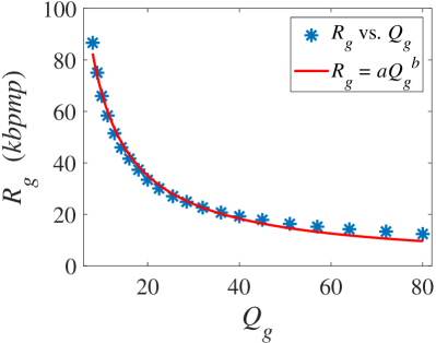
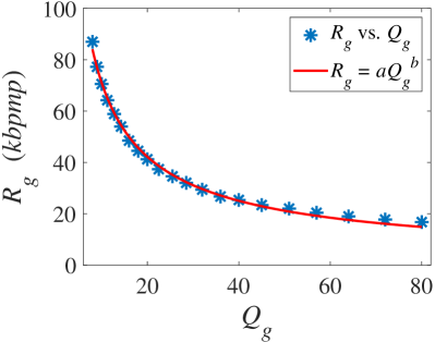
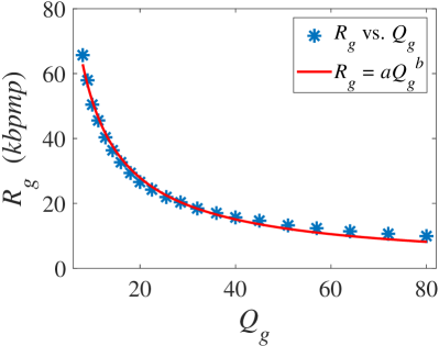
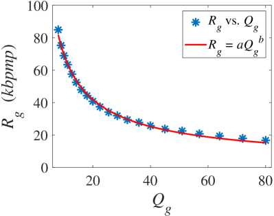
Figure 4: Illustration of the relationship between $R_{g}$ and $Q_{g}$. (a) Phil, (b) Longdress, (c) David, (d) Loot.

From this figure, we can observe that the $R_{g}$ model (14) is appropriate. This is confirmed by Table IV, which shows that the SCCs between the actual $R_{g}$ and the fitted values are always larger than or equal to 0.99.

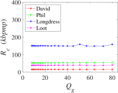
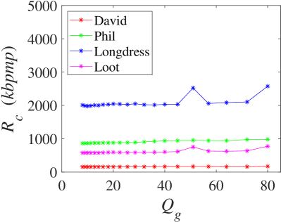
Figure 5: Influence of $Q_{g}$ on $R_{c}$. (a) $Q_{c}$=80, $Q_{g}=8,9,\dots,80$; (b) $Q_{c}$=8, $Q_{g}=8,9,\dots,80$.

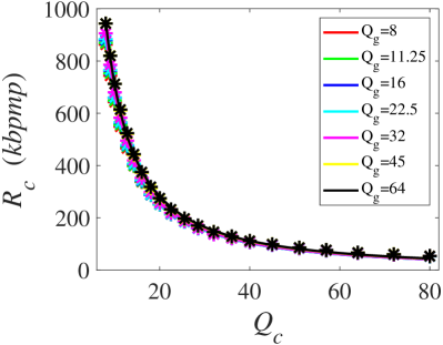
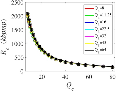
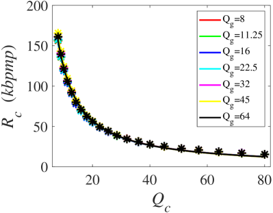
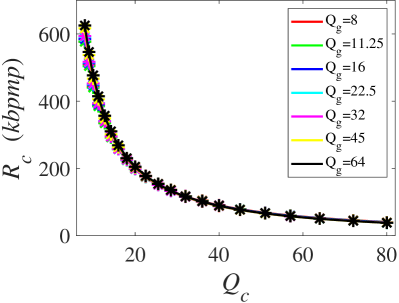
Figure 6: Illustration of the relationship between $R_{c}$ and $Q_{c}$ ($R_{c}=\gamma_{c}Q_{c}^{\theta_{c}}$). (a) Phil, (b) Longdress, (c) David, (d) Loot.

Table IV: Verification of $R_{g}$ Model (14)

Point Cloud	SCC	RMSE (kbpmp)	$\rm Rate_{max}$ (kbpmp)	NRMSE
Andrew	0.99	1.53	75.89	0.02
David	0.99	1.33	65.66	0.02
Phil	0.99	1.93	86.64	0.02
Ricardo	0.99	1.40	67.48	0.02
Longdress	1.00	1.21	86.99	0.01
Loot	1.00	1.23	84.89	0.01
Queen	1.00	1.11	69.23	0.02
Redandblack	1.00	1.53	102.74	0.01

Because the bitrate of a 3D point cloud is typically very large, the RMSE seems to be large. Therefore, we also calculated the normalized RMSE to illustrate the fitting error effectively. The normalized RMSE ($NRMSE$) is defined as

$$NRMSE =\frac{RMSE}{Rate_{\max}},$$ (15)

where $Rate_{\max}$ is the maximum bitrate. Table IV shows that the NRMSE is as low as 0.01, which confirms that (14) is accurate.

To study the effect of $Q_{g}$ on $R_{c}$, we compressed the color information with a fixed $Q_{c}$ and multiple $Q_{g}$s. The results, shown in Fig. 5, indicate that the effect of $Q_{g}$ on $R_{c}$ is negligible. This is also confirmed by Fig. 6, which shows $R_{c}$ as a function of $Q_{c}$ for various $Q_{g}$s.

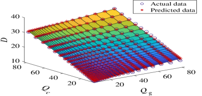
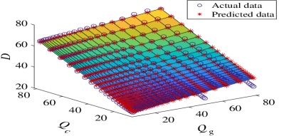
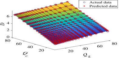
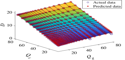
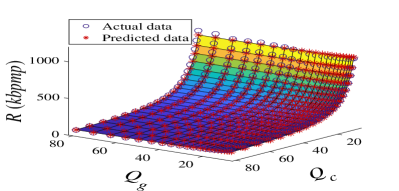
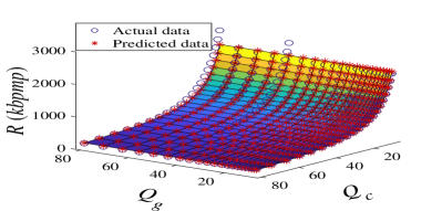
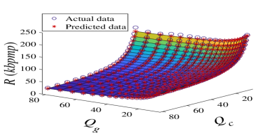
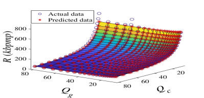
Figure 7: Illustration of the accuracy of the $R$ model (17) and $D$ model (12). (a)-(d): accuracy of the $D$ model (12) for Phil, Longdress, David, and Loot, (e)-(f): accuracy of the $R$ model (17) for Phil, Longdress, David, and Loot.

Thus, for simplicity, we can assume that $R_{c}$ is only affected by $Q_{c}$. Moreover, Fig. 6 suggests that the exponential model

$$R_{c}=\gamma_{c}Q_{c}^{\theta_{c}},$$ (16)

where $\gamma_{c}$ and $\theta_{c}$ are model parameters is appropriate to describe the relationship between $Q_{c}$ and $R_{c}$. This is confirmed in Table V, which shows that the SCC of the relationship between $R_{c}$ and $Q_{c}$ is always greater than or equal to 0.98, while the NRMSE is always smaller than 0.03.

Table V: Verification of $R_{c}$ Model (16)

Point Cloud	SCC	RMSE (kbpmp)	$\rm Rate_{max}$ (kbpmp)	NRMSE
Andrew	1.00	21.78	1192.01	0.02
David	1.00	2.59	172.32	0.02
Phil	0.99	19.10	983.27	0.02
Ricardo	0.99	3.41	179.67	0.02
Longdress	0.98	76.67	2576.12	0.03
Loot	0.98	20.96	774.43	0.03
Queen	0.99	15.94	732.89	0.02
Redandblack	0.99	30.21	1182.12	0.03

Accordingly, (13) can be rewritten as

$$R =R_{g}+R_{c}$$ (17)

$$=\gamma_{g}Q_{g}^{\theta_{g}}+\gamma_{c}Q_{c}^{\theta_{c}}.$$

Different from our previous work [8], the rate of color and geometry are considered separately in this paper, which may lead to more accurate bit allocation result. Table VI validates (17) by showing that the SCC was always greater than or equal to 0.99, and the NRMSE was always smaller than or equal to 0.03.

Table VI: Accuracy of Rate Model (17)

Point Cloud	SCC	RMSE (kbpmp)	$\rm Rate_{max}$ (kbpmp)	NRMSE
Andrew	1.00	17.85	1202.71	0.01
David	1.00	2.97	221.89	0.01
Phil	1.00	17.22	995.64	0.02
Ricardo	0.99	3.94	228.18	0.02
Longdress	0.99	71.07	2592.90	0.03
Loot	0.99	20.36	791.11	0.03
Queen	1.00	11.60	745.44	0.02
Redandblack	0.99	29.30	1201.44	0.02

Finally, Fig. 7 illustrates the accuracy of models (17) and (12) by comparing the actual values to the values predicted by the models.

III Model-based Optimal Bit Allocation Algorithm

Based on the analysis in Section II, the optimal bit allocation problem (1) can be converted to the problem of finding the optimal solution of the constrained optimization problem

$$\min_{(\emph{$Q_{g}$},\emph{$Q_{c}$})} \quad aQ_{g}+bQ_{c}+c$$ (18)

$$\mathrm{s.t.} \gamma_{g}Q_{g}^{\theta_{g}}+\gamma_{c}Q_{c}^{\theta_{c}}\leq\emph{$R_{T}$}.$$

To solve (18), we first need to determine the model parameters $a$, $b$, $c$, $\gamma_{g}$, $\theta_{g}$, $\gamma_{c}$, and $\theta_{c}$. This is done by encoding the 3D point cloud with three different pairs of quantization steps ($Q_{g,1}$,$Q_{c,1}$), ($Q_{g,2}$,$Q_{c,2}$), ($Q_{g,3}$,$Q_{c,3}$) and solving the systems of equations (19) and (20):

$$\begin{cases}D_{1}&=aQ_{g,1}+bQ_{c,1}+c\\ D_{2}&=aQ_{g,2}+bQ_{c,2}+c\\ D_{3}&=aQ_{g,3}+bQ_{c,3}+c\end{cases}$$ (19)

$$\begin{aligned} \begin{cases}R_{g,1}&=\gamma_{g}Q_{g,1}^{\theta_{g}}\\ R_{g,2}&=\gamma_{g}Q_{g,2}^{\theta_{g}}\\ R_{c,1}&=\gamma_{c}Q_{c,1}^{\theta_{c}}\\ R_{c,2}&=\gamma_{c}Q_{c,2}^{\theta_{c}}\end{cases}\end{aligned},$$ (20)

where $D_{1}$, $D_{2}$, $D_{3}$ are the corresponding distortions and $R_{g,1}$, $R_{g,2}$, $R_{c,1}$, $R_{c,2}$ are the corresponding geometry and color bitrates, respectively. Because both the objective function and the constraint function in (18) are convex, the optimal quantization steps, $Q_{g,opt}$ and $Q_{c,opt}$ can be obtained by using an interior point method [43]. In this method, the convex optimization problem is first converted to an unconstrained optimization problem using a logarithmic barrier function [44]:

$$\begin{aligned} \min_{(\emph{$Q_{g}$},\emph{$Q_{c}$})}(aQ_{g}+bQ_{c}+c)-\mu\log[-(\gamma_{g}Q_{g}^{\theta_{g}}+\gamma_{c}Q_{c}^{\theta_{c}}-R_{T})]\end{aligned},$$ (21)

where $\mu$ is the barrier parameter. The details of the interior point method are as follows:
Input: a barrier parameter $\mu>0$, a decline factor $\eta<1$ and          a desired level of accuracy $\epsilon>0$.
Output: ($Q_{g,opt}$, $Q_{c,opt}$), an optimal solution to (18).
Initialization: $k=0$, $(Q_{g,opt},Q_{c,opt})=(Q^{(k)}_{g},Q^{(k)}_{c})=$
                 $(80,80)$, $\mu^{(k)}=\mu$.
While $\mu^{(k)}\geq\epsilon$ :
   Step 1: compute $(Q_{g,opt},Q_{c,opt})$ as solution to (21) using
            Newton’s method initialized with $(Q_{g},Q_{c})=$
            $(Q^{(k)}_{g},Q^{(k)}_{c})$;
   Step 2: update $k=k+1$, $(Q^{(k)}_{g},Q^{(k)}_{c})=(Q_{g,opt},Q_{c,opt})$,
             $\mu^{(k)}=\eta\mu^{(k-1)}$.
The output of the interior point method is subsequently rounded to obtain a solution that belongs to the finite set of discrete quantization steps used by the V-PCC coder. While rounding makes the solution practical for coding, it may lead to a slight violation of the constraint on the target bitrate.

Unlike exhaustive search, the proposed algorithm does not necessarily find an optimal solution to the original problem (1). This is not only due to rounding but also because our analytical rate and distortion models are only approximations. However, the experimental results (see Section IV) show that the rate-distortion performance of the proposed algorithm is very close to that of exhaustive search.

The flowchart of the proposed bit allocation algorithm is shown in Fig. 8.

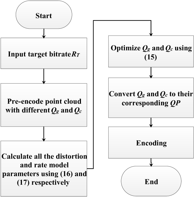
Figure 8: Flow chart of the proposed bit allocation algorithm for geometry and color information.

IV Experimental Results

In this section, we evaluate the accuracy, rate-distortion performance, and time complexity of the proposed bit allocation algorithm. We implemented the proposed algorithm in the test model category 2 version 1.0 (TMC2) [37], which uses High Efficiency Video Coding Test Model Version 16.16 (HM16.16) [45] to compress the generated geometry and color video frames. The barrier parameter $\mu$, decline factor $\eta$, and level of accuracy $\epsilon$ were set to 0.1, $10^{-6}$, and $10^{-10}$, respectively. The quality evaluation software PC_error [46] was used to calculate the point-to-point distortion for both color and geometry. The performance of the proposed algorithm was evaluated on the eight 3D point cloud sequences [47] [48] shown in Fig. 9.

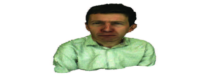
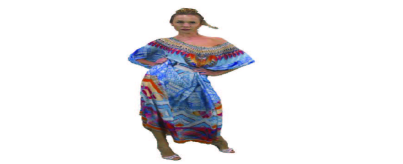
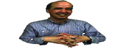
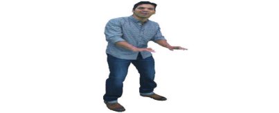
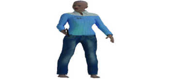
Figure 9: 3D point cloud sequences used in the experiments. (a) Andrew, (b) Longdress, (c) Phil, (d) Redandblack, (e) Ricardo, (f) Loot, (g) David, (h) Queen.

Table VII: Bit Allocation Accuracy for ESA and PBA ($\omega$=0.25) using the bitrate error ($BE$) and the QP error ($QPE$).

Point Cloud	Target Bitrate    ($kbpmp$)	ESA				PBA				BE(%)		$\left|\Delta BE\right|$	QPE
		$QP_{g}$	$QP_{c}$	Bitrate ($kbpmp$)		$QP_{g}$	$QP_{c}$	Bitrate ($kbpmp$)		ESA	PBA
Andrew	240	27	33	232.7		27	33	232.7		3.0	3.0	0.0	0
	450	22	29	444.5		22	29	444.5		1.2	1.2	0.0	0
	600	22	27	594.2		22	27	594.2		1.0	1.0	0.0	0
	760	22	26	683.4		22	25	786.0		10.1	3.4	6.7	1
	1070	22	23	1019.1		22	23	1019.1		4.8	4.8	0.0	0
Phil	240	26	32	237.5		26	32	237.5		1.1	1.1	0.0	0
	450	22	28	423.8		22	28	423.8		5.8	5.8	0.0	0
	600	22	26	552.8		22	25	635.6		7.9	5.9	2.0	1
	760	22	24	729.5		22	24	729.5		4.0	4.0	0.0	0
	1070	22	22	949.4		22	22	949.4		11.3	11.3	0.0	0
Longdress	240	30	40	236.6		30	40	236.6		1.4	1.4	0.0	0
	450	24	35	449.4		24	35	449.4		0.1	0.1	0.0	0
	600	22	33	585.9		22	33	585.9		2.3	2.3	0.0	0
	760	22	31	752.4		22	31	752.4		1.0	1.0	0.0	0
	1070	22	28	1067.4		22	28	1067.4		0.2	0.2	0.0	0
Redandblack	240	29	34	238.2		31	34	230.2		0.8	4.1	3.3	2
	450	23	29	448.0		25	29	429.6		0.5	4.5	4.0	2
	600	22	27	572.2		22	27	572.2		4.6	4.6	0.0	0
	760	22	25	721.6		22	25	721.6		5.1	5.1	0.0	0
	1070	22	22	1011.4		22	22	1011.4		5.5	5.5	0.0	0
David	70	33	31	69.7		36	30	72.7		0.4	3.8	3.4	4
	86	31	29	86.0		34	29	80.9		0.0	5.9	5.9	3
	96	31	28	93.3		33	28	90.5		2.8	5.7	2.9	2
	180	26	23	176.4		27	23	171.8		2.0	4.6	2.6	1
	224	22	22	221.9		22	22	221.9		0.9	0.9	0.0	0
Ricardo	70	36	31	69.0		32	32	69.5		1.4	0.6	0.8	5
	86	30	30	84.6		30	30	84.6		1.6	1.6	0.0	0
	96	29	29	94.7		29	29	94.7		1.3	1.3	0.0	0
	180	24	24	176.5		23	24	182.4		1.9	1.4	0.5	1
	224	23	22	219.9		22	22	228.2		1.8	1.9	0.1	1
Loot	70	42	40	69.6		40	40	70.2		0.6	0.4	0.2	2
	86	36	39	84.5		38	38	93.9		1.8	9.2	7.4	3
	96	35	38	94.8		37	37	100.6		1.2	4.8	3.6	3
	180	35	32	178.9		31	32	188.6		0.6	4.8	4.2	4
	224	28	31	223.7		29	31	220.6		0.1	1.5	1.4	1
Queen	70	34	42	68.2		37	42	65.8		2.6	6.0	3.4	3
	86	30	41	84.2		30	42	77.3		2.1	10.1	8.0	1
	96	27	41	94.3		29	41	89.0		1.8	7.3	5.5	2
	180	22	36	171.9		22	35	184.9		4.5	2.7	1.8	1
	224	22	33	220.6		22	33	220.6		1.5	1.5	0.0	0
Average										2.6	3.7	1.7	1.1

Table VIII: Bit Allocation Accuracy for ESA and PBA ($\omega$=0.5) using the bitrate error ($BE$) and the QP error ($QPE$).

Point Cloud	Target Bitrate    ($kbpmp$)	ESA				PBA				BE(%)		$\left|\Delta BE\right|$	QPE
		$QP_{g}$	$QP_{c}$	Bitrate ($kbpmp$)		$QP_{g}$	$QP_{c}$	Bitrate ($kbpmp$)		ESA	PBA
Andrew	240	27	33	232.7		27	33	232.7		3.0	3.0	0.0	0
	450	22	29	444.5		22	29	444.5		1.2	1.2	0.0	0
	600	22	27	594.2		22	27	594.2		1.0	1.0	0.0	0
	760	22	26	683.4		22	25	786.0		10.1	3.4	6.7	1
	1070	22	23	1019.1		22	23	1019.1		4.8	4.8	0.0	0
Phil	240	26	32	237.5		26	32	237.5		1.1	1.1	0.0	0
	450	22	28	423.8		22	28	423.8		5.8	5.8	0.0	0
	600	22	26	552.8		22	25	635.6		7.9	5.9	2.0	1
	760	22	24	729.5		22	24	729.5		4.0	4.0	0.0	0
	1070	22	22	949.4		22	22	949.4		11.3	11.3	0.0	0
Longdress	240	30	40	236.6		30	40	236.6		1.4	1.4	0.0	0
	450	24	35	449.4		24	35	449.4		0.1	0.1	0.0	0
	600	22	33	585.9		22	33	585.9		2.3	2.3	0.0	0
	760	22	31	752.4		22	31	752.4		1.0	1.0	0.0	0
	1070	22	28	1067.4		22	28	1067.4		0.2	0.2	0.0	0
Redandblack	240	29	34	238.2		30	34	234.4		0.8	2.3	1.5	1
	450	23	29	448.0		24	29	440.1		0.5	2.2	1.7	1
	600	22	27	572.2		22	27	572.2		4.6	4.6	0.0	0
	760	22	25	721.6		22	25	721.6		5.1	5.1	0.0	0
	1070	22	22	1011.4		22	22	1011.4		5.5	5.5	0.0	0
David	70	33	31	69.7		34	31	68.5		0.4	2.2	1.8	1
	86	31	29	86.0		32	29	83.6		0.0	2.8	2.8	1
	96	31	28	93.3		31	28	93.3		2.8	2.8	0.0	0
	180	26	23	176.4		25	23	181.5		2.0	0.9	1.1	1
	224	22	22	221.9		22	22	221.9		0.9	0.9	0.0	0
Ricardo	70	32	32	69.5		31	32	70.1		0.6	0.1	0.5	1
	86	30	30	84.6		29	30	87.6		1.6	1.9	0.3	1
	96	29	29	94.7		28	29	97.8		1.3	1.9	0.6	1
	180	24	24	176.5		22	24	189.8		1.9	5.5	3.6	2
	224	23	22	219.9		22	22	228.2		1.8	1.9	0.1	1
Loot	70	42	40	69.6		39	40	71.7		0.6	2.5	1.9	3
	86	36	39	84.5		37	38	90.2		1.8	4.9	3.1	2
	96	35	38	94.8		36	38	92.4		1.2	3.8	2.6	1
	180	29	33	179.6		30	33	175.0		0.2	2.8	2.6	1
	224	28	31	223.7		28	31	223.7		0.1	0.1	0.0	0
Queen	70	34	42	68.2		37	42	65.8		2.6	6.0	3.4	3
	86	30	41	84.2		30	42	77.3		2.1	10.1	8.0	1
	96	27	41	94.3		28	41	92.0		1.8	4.1	2.3	1
	180	22	36	171.9		22	35	184.9		4.5	2.7	1.8	1
	224	22	33	220.6		22	33	220.6		1.5	1.5	0.0	0
Average										2.5	3.1	1.2	0.7

Table IX: Rate-PSNR Performance of ESA and PBA

Point Cloud	Target Bitrate ($kbpmp$)	ESA						PBA						BD-PSNR ($dB$)
		Bitrate ($kbpmp$)			PSNR ($dB$)			Bitrate ($kbpmp$)			PSNR ($dB$)			$\omega=0.25$	$\omega=0.5$
		$\omega=0.25$	$\omega=0.5$		$\omega=0.25$	$\omega=0.5$		$\omega=0.25$	$\omega=0.5$		$\omega=0.25$	$\omega=0.5$
Andrew	240	233	233		32.8	34.5		233	233		32.8	34.5
	450	445	445		33.8	35.6		445	445		33.8	35.6
	600	594	594		34.2	36.0		594	594		34.2	36.0		0.00	0.00
	760	683	683		34.4	36.1		786	786		34.5	36.3
	1070	1019	1019		34.8	36.5		1019	1019		34.8	36.5
Phil	240	237	237		34.5	36.3		237	237		34.5	36.3
	450	424	424		35.6	37.3		424	424		35.6	37.3
	600	553	553		36.0	37.7		636	636		36.1	37.9		0.00	0.00
	760	730	730		36.3	38.1		730	730		36.3	38.1
	1070	949	949		36.6	38.3		949	949		36.6	38.3
Longdress	240	237	237		28.8	30.6		237	237		28.8	30.6
	450	449	449		30.5	32.3		449	449		30.5	32.3
	600	586	586		31.2	33.0		586	586		31.2	33.0		0.00	0.00
	760	752	752		31.7	33.4		752	752		31.7	33.4
	1070	1067	1067		32.2	34.0		1067	1067		32.2	34.0
Redandblack	240	238	238		36.0	37.8		230	234		35.9	37.7
	450	448	448		37.7	39.4		430	440		37.6	39.4
	600	572	572		38.3	40.1		572	572		38.3	40.1		0.01	0.00
	760	722	722		38.7	40.5		722	722		38.7	40.5
	1070	1011	1011		39.3	41.0		1011	1011		39.3	41.0
David	70	70	70		42.4	44.1		73	68		42.7	44.1
	86	86	86		43.0	44.8		81	84		42.9	44.7
	96	93	93		43.4	45.1		91	93		43.3	45.1		0.04	0.03
	180	176	176		44.9	46.7		172	182		44.9	46.8
	224	222	222		45.3	47.1		222	222		45.3	47.1
Ricardo	70	69	70		41.8	43.5		70	70		41.8	43.5
	86	85	85		42.3	44.0		85	88		42.3	44.1
	96	95	95		42.6	44.4		95	98		42.6	44.3		0.01	-0.07
	180	177	177		43.9	45.7		182	190		44.0	45.8
	224	220	220		44.3	46.1		228	228		44.3	46.1
Loot	70	70	70		34.0	35.8		70	72		34.1	35.9
	86	84	84		34.7	36.4		94	90		34.9	36.7
	96	95	95		35.1	36.8		101	92		35.3	36.8		0.00	0.05
	180	179	180		37.2	38.9		189	175		37.4	38.9
	224	224	224		37.9	39.7		221	224		37.9	39.7
Queen	70	68	68		30.3	32.0		66	66		29.5	31.2
	86	84	84		31.4	33.2		77	77		31.1	32.8
	96	94	94		32.0	33.7		89	92		31.7	33.5		0.02	-0.01
	180	172	172		33.9	35.7		185	185		34.1	35.9
	224	221	221		34.6	36.4		221	221		34.6	36.4
Average														0.01	0.00

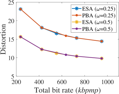
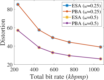
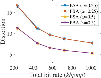
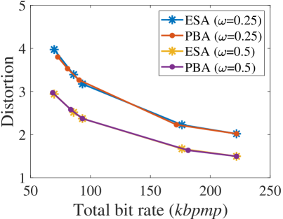
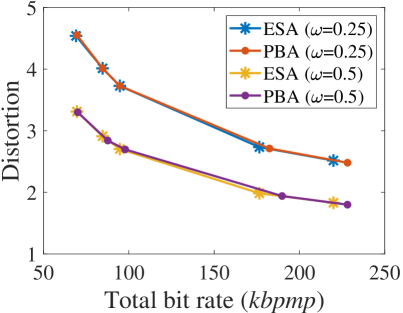
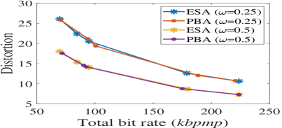
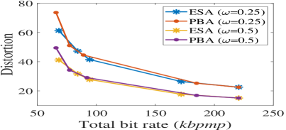
Figure 10: R-D performance of the proposed algorithm (PBA) and exhaustive search (ESA). (a) Andrew, (b)Phil , (c) Longdress, (d) Redandblack, (e) David, (f) Ricardo, (g) Loot, (h) Queen.

Because the color of the 3D point cloud sequences in Figs. 9-9 is more diverse than that of the sequences in Figs. 9-9, we divided the point clouds in Fig. 9 into two groups, a complex 3D point cloud group (Andrew, Longdress, Phil and Redandblack) and a simple 3D point cloud group (Ricardo, Loot, David, and Queen). The performance of exhaustive search was used as the benchmark. In exhaustive search, a 3D point cloud was first encoded by all the possible geometry and color quantization step pairs (ranging from 8 to 80), which correspond to $QP$ values 22, 23, 24, …, 42. Then the subset of admissible pairs (that is, those for which the bitrate is smaller than the target bitrate) was identified. Finally, the pair that gave the smallest distortion was selected from this subset.

In the proposed method, to derive the rate and distortion models, the point clouds were empirically pre-encoded with three geometry-color QP pairs (33, 25), (34, 35), and (24, 33). The distortion model parameters $a$, $b$ and $c$ were computed by solving (19), and the rate model parameters $\gamma_{g}$, $\theta_{g}$, $\gamma_{c}$, and $\theta_{c}$ were obtained by solving (20). Then, given the target bitrate $R_{T}$, the optimal $Q_{g,opt}$ and $Q_{c,opt}$ were obtained by solving (18) using the interior point method.

IV-A Bit Allocation Accuracy of Proposed Algorithm

To evaluate the accuracy of the proposed bit allocation algorithm for the tested point clouds, we set different target bitrates according to the geometry and color characteristics of each sequence to cover different compression levels. For the complex 3D point clouds, the common target bitrates are 240 kbpmp, 450 kbpmp, 600 kbpmp, 760 kbpmp, and 1070 kbpmp. For the simple 3D point cloud group, the target bitrates are 70 kbpmp, 86 kbpmp, 96 kbpmp, 180 kbpmp, and 224 kbpmp. In practical applications, the target bitrate for geometry and color can be obtained by subtracting the bitrate of the occupancy map and the auxiliary information, which can be obtained by pre-encoding. To evaluate the bit allocation accuracy, we used the bitrate error ($BE$), defined as

$$BE =\frac{\left|B_{actual}-B_{target}\right|}{B_{target}}\times 100\%,$$ (22)

where $B_{actual}$ is the actual bitrate and $B_{target}$ represents the target bitrate. The lower the BE, the more accurate the algorithm. Because the proposed bit allocation algorithm allocated the bits for geometry and color components by selecting the QPs, QP error ($QPE$) was also used to measure the performance as follows:

$$QPE =\left|QP_{g,PBA}-QP_{g,ESA}\right|+\left|QP_{c,PBA}-QP_{c,ESA}\right|,$$ (23)

where $QP_{g,PBA}$ and $QP_{c,PBA}$ denote the geometry and color QPs obtained from the proposed algorithm, and $QP_{g,ESA}$ and $QP_{c,ESA}$ represent the geometry and color QPs obtained from exhaustive search.

Table VII and Table VIII show the $BE$ and $QPE$ of the proposed bit allocation algorithm (PBA) and exhaustive search (ESA) for different values of $\omega$ (0.25 and 0.5). Note that ESA produces an optimal solution but has a much higher computational cost. As shown in Table VII and Table VIII, the $BE$ of ESA was as small as zero, while its average was 2.6% and 2.5% when $\omega$ was set to 0.25 and 0.5, respectively. For PBA, $BE$ was as low as 0.1%, while its average was about 3.7% and 3.1% when $\omega$ was set to 0.25 and 0.5, respectively. The average absolute difference in BE between ESA and PBA was only 1.7% and 1.2% for $\omega=0.25$ and 0.5, respectively. On the other hand, the average $QPE$ was only 1.1 when $\omega$ was set to 0.25 and only 0.7 when $\omega$ was set to 0.5. In 50% of the cases, our algorithm (PBA) found the same solution as exhaustive search (ESA), so the BE of the two algorithms was the same. In the remaining cases, our algorithm found a suboptimal solution (see the discussion at the end of Section III), which had a higher BE in 36.25% of the cases and a lower one in 13.75% of the cases.

IV-B Rate-Distortion Performance

In addition to bit allocation accuracy, the rate-distortion performance should also be taken into account. After determining the coding parameters with ESA and PBA, we compressed the point clouds and computed their respective distortion and peak signal-to-noise ratio (PSNR) using the PC_error reference software [46].

Fig. 10 shows the distortion $D=\omega D_{g}+(1-\omega)D_{c}$ as a function of the bitrate (in $kbpmp$) for PBA and ESA. We can see that the rate-distortion performance of the proposed algorithm was very close to that of exhaustive search.

In addition to the distortion (measured in MSE), we used the BD-PSNR  [49] to compare the performance of the two algorithms. In general, it is necessary to normalize with respect to the peak value when converting MSE into $PSNR$. However, the peak values of geometry and color are completely different. To calculate the $PSNR$ of the reconstructed 3D point cloud reasonably, the geometry and color values were both normalized to [0,1]. Hence, the $PSNR$ of the reconstructed 3D point cloud was calculated as:

$$PSNR =10\log_{10}\left[\frac{1}{NMSE(NMSE_{g},NMSE_{c})}\right],$$ (24)

where $NMSE_{g}$ and $NMSE_{c}$ are the normalized geometry and color (Y channel) distortion (i.e., $D_{g}$ and $D_{c}$), respectively and $NMSE(NMSE_{g},NMSE_{c})=\omega NMSE_{g}+(1-\omega)NMSE_{c}$.

Table IX shows that there is almost no BD-PSNR degradation of PBA when $\omega=0.5$. Interestingly, an average 0.01 dB BD-PSNR gain was achieved when $\omega=0.25$. The main reason is that ESA is optimal for the distortion $D=\omega D_{g}+(1-\omega)D_{c}$ but not necessarily optimal for the PSNR (24).

IV-C Complexity Comparison

We run the experiments on a PC with a 3.40 GHz Intel Core i7 Processor and 8.00 GB RAM and used the encoding time to evaluate the time complexity. The ratio between the encoding time of PBA and that of ESA was used to define the complexity quotient (CQ) as

$$CQ =\frac{T_{PBA}}{T_{ESA}}\times 100\%,$$ (25)

where $T_{PBA}$ and $T_{ESA}$ denote the encoding time of PBA and ESA, respectively. The time complexity of ESA and PBA mainly depends on the pre-encoding times. ESA needs to pre-encode the 3D point cloud for all possible combinations of QPs for the geometry and color components. Because both the geometry and color QP search range was [22, 42] with a search step size of 1, a 3D point cloud needs to be encoded $21\times 21=441$ times to find the optimal $Q_{g}$ and $Q_{c}$ with ESA. In contrast, only three pre-encodings were required by PBA to compute the model parameters. As the time complexity of the interior point method is very small compared to the pre-encoding procedure (for example the time spent to obtain the optimal $Q_{g}$ and $Q_{c}$ by the interior point method was only 1.47 s for the $Andrew$ point cloud, while a single pre-encoding required 120.96 s), the time complexity of PBA was only about 0.68% of that of ESA, as shown in Table X.

Table X: Complexity Comparison for ESA and PBA

Point Cloud	Encoding Time ($s$)		CQ(%)
	ESA	PBA
Andrew	53342.84	364.08	0.68
Phil	56716.51	366.50	0.65
Longdress	38476.52	247.17	0.64
Redandblack	33958.65	234.23	0.69
David	50537.59	335.58	0.66
Ricardo	38867.25	251.00	0.65
Loot	35673.09	256.62	0.72
Queen	41749.56	298.17	0.71
Average			0.68

V Conclusion

This paper presented a model-based joint bit allocation algorithm for the V-PCC encoder. To reduce the time complexity of exhaustive search as well as preserve its rate-distortion performance, we first derived rate and distortion models for point clouds through theoretical analysis and statistical validation. Based on the derived rate and distortion models, the optimal bit allocation problem was formulated as a convex constrained optimization problem and solved by an interior point method. Model parameters were calculated by pre-encoding a 3D point cloud only three times. Experimental results showed that the bit allocation accuracy and the rate-distortion performance of the PBA were very close to those of exhaustive search at only 0.68% of its computational cost. As future work, we plan to use our rate and distortion models to develop a rate control algorithm for 3D point clouds.

Appendix A

From the law of large numbers [50], the average value of the coding error of the point cloud approximates to its expectation value. Thus, (6) can be written as

$$e^{B,A}_{c} \approx E\{(\textbf{\emph{C}}_{v}-\textbf{\emph{C}}_{v^{*}})^{2}\},$$ (26)

where $E\{.\}$ denotes the expectation operator, $\textbf{\emph{C}}_{v}$ is the random variable corresponding to the color of the point cloud $A$, and $\textbf{\emph{C}}_{v^{*}}$ is the random variable corresponding to the color of the point cloud $B$. In the V-PCC encoder, the color information of the points is reassigned to the reconstructed geometry information [37]. Let $\textbf{\emph{C}}_{v^{g}}$ denote the reassigned color that is not compressed. Then (26) can be rewritten as:

$$e^{B,A}_{c} \approx E\{(\textbf{\emph{C}}_{v}-\textbf{\emph{C}}_{v^{g}}+\textbf{\emph{C}}_{v^{g}}-\textbf{\emph{C}}_{v^{*}})^{2}\}$$ (27)

$$=E\{(\textbf{\emph{C}}_{v}-\textbf{\emph{C}}_{v^{g}})^{2}\}+E\{(\textbf{\emph{C}}_{v^{g}}-\textbf{\emph{C}}_{v^{*}})^{2}\}$$

$$\quad+2E\{(\textbf{\emph{C}}_{v}-\textbf{\emph{C}}_{v^{g}})(\textbf{\emph{C}}_{v^{g}}-\textbf{\emph{C}}_{v^{*}})\},$$

where $E\{(\textbf{\emph{C}}_{v}-\textbf{\emph{C}}_{v^{g}})^{2}\}$ represents the color distortion induced only by $Q_{g}$, and $E\{(\textbf{\emph{C}}_{v^{g}}-\textbf{\emph{C}}_{v^{*}})^{2}\}$ represents the color distortion induced only by $Q_{c}$. Because $(\textbf{\emph{C}}_{v}-\textbf{\emph{C}}_{v^{g}})$ and $(\textbf{\emph{C}}_{v^{g}}-\textbf{\emph{C}}_{v^{*}})$ can be thought of as two independent random variables, $E\{(\textbf{\emph{C}}_{v}-\textbf{\emph{C}}_{v^{g}})(\textbf{\emph{C}}_{v^{g}}-\textbf{\emph{C}}_{v^{*}})\}$ approximates to zero [51] [52]. Accordingly, (27) can be further written as

$$e^{B,A}_{c} =f^{B,A}_{g}(Q_{g})+f^{B,A}_{c}(Q_{c}),$$ (28)

where $f^{B,A}_{g}(Q_{g})=E\{(\textbf{\emph{C}}_{v}-\textbf{\emph{C}}_{v^{g}})^{2}\}$ and $f^{B,A}_{c}(Q_{c})=E\{(\textbf{\emph{C}}_{v^{g}}-\textbf{\emph{C}}_{v^{*}})^{2}\}$.

References

- [1] Y. Cui, S. Schuon, S. Thrun, D. Stricker, and C. Theobalt, “Algorithms for 3D shape scanning with a depth camera,” IEEE Transactions on Pattern Analysis and Machine Intelligence, vol. 35, no. 5, pp. 1039–1050, May 2013.
- [2] R. B. Rusu and S. Cousins, “3D is here: Point cloud library (PCL),” in 2011 IEEE international conference on robotics and automation. IEEE, 2011, pp. 1–4.
- [3] E. Vlachos, A. S. Lalos, A. Spathis-Papadiotis, and K. Moustakas, “Distributed consolidation of highly incomplete dynamic point clouds based on rank minimization,” IEEE Transactions on Multimedia, vol. 20, no. 12, pp. 3276–3288, Dec 2018.
- [4] J. Chen, C. Lin, P. Hsu, and C. Chen, “Point cloud encoding for 3D building model retrieval,” IEEE Transactions on Multimedia, vol. 16, no. 2, pp. 337–345, Feb 2014.
- [5] X. Chen, H. Ma, J. Wan, B. Li, and T. Xia, “Multi-view 3D object detection network for autonomous driving,” in Proceedings of the IEEE Conference on Computer Vision and Pattern Recognition, 2017, pp. 1907–1915.
- [6] W. Oropallo, L. A. Piegl, P. Rosen, and K. Rajab, “Point cloud slicing for 3-D printing,” Computer-Aided Design and Applications, vol. 15, no. 1, pp. 90–97, 2018.
- [7] Y. Park, V. Lepetit, and W. Woo, “Multiple 3d object tracking for augmented reality,” in Proceedings of the 7th IEEE/ACM International Symposium on Mixed and Augmented Reality. IEEE Computer Society, 2008, pp. 117–120.
- [8] Q. Liu, H. Yuan, J. Hou, H. Liu, and R. Hamzaoui, “Model-based encoding parameter optimization for 3D point cloud compression,” in 2018 Asia-Pacific Signal and Information Processing Association Annual Summit and Conference (APSIPA ASC). IEEE, 2018, pp. 1981–1986.
- [9] S. Schwarz, M. Preda, V. Baroncini, M. Budagavi, P. Cesar, P. A. Chou, R. A. Cohen, M. Krivokuća, S. Lasserre, Z. Li et al., “Emerging mpeg standards for point cloud compression,” IEEE Journal on Emerging and Selected Topics in Circuits and Systems, vol. 9, no. 1, pp. 133–148, 2018.
- [10] R. A. Cohen, D. Tian, and A. Vetro, “Point cloud attribute compression using 3-D intra prediction and shape-adaptive transforms,” in 2016 Data Compression Conference (DCC). IEEE, 2016, pp. 141–150.
- [11] C. Zhang, D. Florencio, and C. Loop, “Point cloud attribute compression with graph transform,” in 2014 IEEE International Conference on Image Processing (ICIP). IEEE, 2014, pp. 2066–2070.
- [12] R. A. Cohen, D. Tian, and A. Vetro, “Attribute compression for sparse point clouds using graph transforms,” in 2016 IEEE International Conference on Image Processing (ICIP). IEEE, 2016, pp. 1374–1378.
- [13] P. de Oliveira Rente, C. Brites, J. Ascenso, and F. Pereira, “Graph-based static 3D point clouds geometry coding,” IEEE Transactions on Multimedia, vol. 21, no. 2, pp. 284–299, Feb 2019.
- [14] R. L. de Queiroz and P. A. Chou, “Compression of 3D point clouds using a region-adaptive hierarchical transform,” IEEE Transactions on Image Processing, vol. 25, no. 8, pp. 3947–3956, 2016.
- [15] G. P. Sandri, P. A. Chou, M. Krivokuća, and R. L. de Queiroz, “Integer alternative for the region-adaptive hierarchical transform,” IEEE Signal Processing Letters, vol. 26, no. 9, pp. 1369–1372, 2019.
- [16] D. Flynn and S. Lasserre, “Report on upsampled transform domain prediction in RAHT,” ISO/IEC JTC1/SC29/WG11 MPEG M49380, 2019, Jul.
- [17] M. Khaled, A. Tourapis, J. Kim, F. Robinet, V. Valentin, and Y. Su, “Lifting scheme for lossy attribute encoding in TMC1,” ISO/IEC JTC1/SC29/WG11 MPEG M42640, 2018, Apr.
- [18] P. A. Chou and R. L. de Queiroz, “Gaussian process transforms,” in 2016 IEEE International Conference on Image Processing (ICIP). IEEE, 2016, pp. 1524–1528.
- [19] R. L. de Queiroz and P. A. Chou, “Transform coding for point clouds using a gaussian process model,” IEEE Transactions on Image Processing, vol. 26, no. 7, pp. 3507–3517, 2017.
- [20] S. Gu, J. Hou, H. Zeng, H. Yuan, and K.-K. Ma, “3D point cloud attribute compression using geometry-guided sparse representation,” IEEE Transactions on Image Processing, vol. 29, pp. 796–808, 2019.
- [21] J. Hou, L.-P. Chau, Y. He, and P. A. Chou, “Sparse representation for colors of 3D point cloud via virtual adaptive sampling,” in 2017 IEEE International Conference on Acoustics, Speech and Signal Processing (ICASSP). IEEE, 2017, pp. 2926–2930.
- [22] Y. Shao, Q. Zhang, G. Li, and Z. Li, “Hybrid point cloud attribute compression using slice-based layered structure and block-based intra prediction,” arXiv preprint arXiv:1804.10783, 2018.
- [23] R. Mekuria, K. Blom, and P. Cesar, “Design, implementation, and evaluation of a point cloud codec for tele-immersive video,” IEEE Transactions on Circuits and Systems for Video Technology, vol. 27, no. 4, pp. 828–842, 2016.
- [24] C. Tu, E. Takeuchi, C. Miyajima, and K. Takeda, “Compressing continuous point cloud data using image compression methods,” in 2016 IEEE 19th International Conference on Intelligent Transportation Systems (ITSC). IEEE, 2016, pp. 1712–1719.
- [25] J. Hou, L. Chau, N. Magnenat-Thalmann, and Y. He, “Compressing 3-D human motions via keyframe-based geometry videos,” IEEE Transactions on Circuits and Systems for Video Technology, vol. 25, no. 1, pp. 51–62, Jan 2015.
- [26] J. Hou, L. Chau, M. Zhang, N. Magnenat-Thalmann, and Y. He, “A highly efficient compression framework for time-varying 3-D facial expressions,” IEEE Transactions on Circuits and Systems for Video Technology, vol. 24, no. 9, pp. 1541–1553, Sep. 2014.
- [27] J. Hou, L. Chau, Y. He, M. Zhang, and N. Magnenat-Thalmann, “Rate-distortion model based bit allocation for 3-D facial compression using geometry video,” IEEE Transactions on Circuits and Systems for Video Technology, vol. 23, no. 9, pp. 1537–1541, Sep. 2013.
- [28] J. Xia, D. T. P. Quynh, Y. He, X. Chen, and S. C. H. Hoi, “Modeling and compressing 3-D facial expressions using geometry videos,” IEEE Transactions on Circuits and Systems for Video Technology, vol. 22, no. 1, pp. 77–90, Jan 2012.
- [29] X. Gu, S. J. Gortler, and H. Hoppe, “Geometry images,” in ACM Transactions on Graphics (TOG), vol. 21, no. 3. ACM, 2002, pp. 355–361.
- [30] D. Thanou, P. A. Chou, and P. Frossard, “Graph-based compression of dynamic 3D point cloud sequences,” IEEE Transactions on Image Processing, vol. 25, no. 4, pp. 1765–1778, 2016.
- [31] R. L. de Queiroz and P. A. Chou, “Motion-compensated compression of dynamic voxelized point clouds,” IEEE Transactions on Image Processing, vol. 26, no. 8, pp. 3886–3895, 2017.
- [32] A. Anis, P. A. Chou, and A. Ortega, “Compression of dynamic 3D point clouds using subdivisional meshes and graph wavelet transforms,” in 2016 IEEE International Conference on Acoustics, Speech and Signal Processing (ICASSP). IEEE, 2016, pp. 6360–6364.
- [33] P. A. Chou, O. Nakagami, and E. S.Jang, “Point cloud compression test model for category 1 v0,” ISO/IEC JTC1/SC29/WG11 MPEG N17223, 2017.
- [34] M. Khaled, “PCC test model category 2 v0,” ISO/IEC JTC1/SC29/WG11 MPEG N17248, 2017.
- [35] ——, “PCC test model category 3 v0,” ISO/IEC JTC1/SC29/WG11 MPEG N17249, 2017.
- [36] M. Khaled, P. A. Chou, D. Flynn, M. Krivokuća, O. Nakagami, and T. Sugio, “G-PCC codec description v2,” ISO/IEC JTC1/SC29/WG11 MPEG N18189, 2019.
- [37] K. Mammou, “PCC test model category 2 v1,” ISO/IEC JTC1/SC29/WG11 MPEG, N17348, 2018.
- [38] H. Liu, H. Yuan, Q. Liu, J. Hou, and J. Liu, “A comprehensive study and comparison of core technologies for MPEG 3D point cloud compression,” IEEE Transactions on Broadcasting, 2019, doi: 10.1109/TBC.2019.2957652, to be appeared.
- [39] MPEG. (2017) Test code PCC in 3DG. [Online]. Available: https://github.com/RufaelDev/pcc-mp3dg
- [40] C. T. P. C. Rufael Mekuria, Zhu Li, “Evaluation criteria for pcc (point cloud compression),” ISO/IEC JTC1/SC29/WG11 MPEG, N16332, 2016.
- [41] R. Mekuria, S. Laserre, and C. Tulvan, “Performance assessment of point cloud compression,” in 2017 IEEE Visual Communications and Image Processing (VCIP). IEEE, 2017, pp. 1–4.
- [42] F. Cen, Q. Lu, and W. Xu, “Efficient rate control for intra-frame coding in high efficiency video coding,” in 2014 International Conference on Signal Processing and Multimedia Applications (SIGMAP). IEEE, 2014, pp. 54–59.
- [43] Y. Zhang, “Solving large-scale linear programs by interior-point methods under the matlab environment,” Optimization Methods and Software, vol. 10, no. 1, pp. 1–31, 1998.
- [44] S. Boyd and L. Vandenberghe, Convex optimization. Cambridge University press, 2004.
- [45] JCT-VC. (2017) HEVC test model. [Online]. Available: Available: https: //hevc.hhi.fraunhofer.de/svn/svn_HEVCSoftware
- [46] S. Schwarz and D. Flynn, “Common test conditions for point cloud compression,” ISO/IEC JTC1/SC29/WG11 MPEG, N18175, 2019.
- [47] MPEG, “MPEG point cloud datasets,” vailable: http://mpegfs.int-evry.fr/MPEG/PCC/DataSets/pointCloud/CfP/datasets, 2018, May.
- [48] E. d’Eon, B.Harrison, T. Myers, and P.A.Chou, “8i voxelized full bodies -a voxelized point cloud dataset,” ISO/IEC JTC1/SC29/WG11 MPEG, input document WG11M40059/WG1M74006, Geneva, Jan.2017.
- [49] G. Bjøntegaard, “Calculation of average PSNR differences between RD curves,” ITU-T SC16/Q6, VCEG-M33, 2001, Apr.
- [50] S. Idele, “The law of large numbers: Some issues of interpretation and application for beginners,” Journal of the Royal Statistical Society: Series D (The Statistician), vol. 28, no. 3, pp. 209–217, 1979.
- [51] H. Yuan, Y. Chang, J. Huo, F. Yang, and Z. Lu, “Model-based joint bit allocation between texture videos and depth maps for 3-D video coding,” IEEE Transactions on Circuits and Systems for Video Technology, vol. 21, no. 4, pp. 485–497, 2011.
- [52] F. Shao, G. Jiang, W. Lin, M. Yu, and Q. Dai, “Joint bit allocation and rate control for coding multi-view video plus depth based 3D video,” IEEE Transactions on Multimedia, vol. 15, no. 8, pp. 1843–1854, Dec 2013.