Quantum Rotor Atoms in Light Beams with Orbital Angular Momentum: Highly Accurate Rotation Sensor

Abstract

Atoms trapped in a red detuned retro-reflected Laguerre-Gaussian beam undergo orbital motion within rings whose centers are on the axis of the laser beam. We determine the wave functions, energies and degeneracies of such quantum rotors (QRs), and the microwave transitions between the energy levels are elucidated. We then show how such QR atoms can be used as high-accuracy rotation sensors when the rings are singly-occupied.

Introduction: We show that quantum rotor (QR) atoms (atoms whose motion is constrained to a circular ring) Kuzmenko_19 can be formed in light beams having orbital angular momentum and that they can be used as an extremely high accuracy rotation sensor. QR atoms are trapped in a red-detuned linearly polarized retro-reflected Laguerre-Gaussian (LG) beam Goubau_61 ; Allen_92 ; Clifford_98 ; LG-beam-lens-2004 ; LG-beam-lens-1987 . A line of singly-occupied rings filled with QR atoms can be easily formed (see Fig. 1) Viverit_04 ; Bloch_08 ; Gibbons_08 . Single-occupation and negligible tunneling between rings are important to suppress deleterious spin exchange collisions between QR atoms for sensor applications. The accuracy obtained here suggests that this can be the highest precision rotation sensor proposed so far in the literature.

A LG beam propagating along the $z$-axis with orbital angular momentum $l$ and polarization ${\bf e}_{\alpha}$ can be written in terms of a slowly varying envelope $u_{l,p}(r,\phi,z)$ of the electric field as

$${\bf E}_{\alpha,l,p}({\bf r},t)=u_{l,p}(r,\phi,z)\,e^{i(kz-kz_{0}-\omega t)}\,{\bf e}_{\alpha}+{\mathrm{c.c.}},$$ (1)

with field amplitude mode ${\rm{LG}}_{p}^{l}({\bf r})\equiv u_{l,p}({\bf r})$ Goubau_61 ; Allen_92 ; Clifford_98 ,

$$u_{l,p}(r,\phi,z)=\sqrt{\frac{2p!}{\pi\left({p+\left|l\right|!}\right)}}\frac{{\sqrt{P_{0}/c}}}{{w\left(z\right)}}{\left({\frac{r\sqrt{2}}{w\left(z\right)}}\right)^{\left|l\right|}}\exp\left({-\frac{{{r^{2}}}}{{{w^{2}}\left(z\right)}}}\right)$$ (2)

$$\times L_{p}^{\left|l\right|}\left({\frac{{2{r^{2}}}}{{{w^{2}}\left(z\right)}}}\right)\exp\left({-\frac{{ik{r^{2}}z}}{{2\left({{z^{2}}+z_{R}^{2}}\right)}}}\right)\exp\left({-il\phi}\right)$$

$$\times\exp\left[{i\left({2p+|l|+1}\right){{\tan}^{-1}}\left({\frac{z}{{{z_{R}}}}}\right)}\right].$$

Here $z$ is the longitudinal distance from the beam waist located at $z=0$, $P_{0}$ is the laser beam power, $w_{0}$ is the beam waist at $z=0$, $R(z)=z(1+(z_{R}/z)^{2})$ is the radius of curvature of the beam wavefront, $w(z)=w_{0}(1+(z/z_{R}))^{1/2}$ is the radius at which the beam intensity falls to $1/e$ of its axis value at $z$, $z_{R}=\pi w_{0}^{2}/\lambda$ is the Rayleigh range for the laser with wavelength $\lambda=2\pi/k$ where $k=\omega/c$ is the wavenumber, $0<z_{0}<\lambda/2$ is a phase parameter, $L_{p}^{\left|l\right|}(x)$ is the associated Laguerre polynomial, $\phi$ is the azimuthal angle, and $\tan^{-1}\left(z/z_{R}\right)$ is the Gouy phase. Figure 1 is a schematic diagram of a retro-reflected LG beam propagating along the $z$-axis, and Fig. 1 shows superposition of two counter-propagating beams that form a standing wave along the $z$-axis. The slowly varying envelope $u_{l,p}(r,\phi,z)$ of the counter-propagating (cp) standing wave has the form

$${\bf E}^{\mathrm{cp}}_{\alpha,l,p}({\bf r},t)=u_{l,p}(r,\phi,z)\,{\bf e}_{\alpha}\,(e^{i(kz-kz_{0}-\omega t)}+e^{i(-kz+kz_{0}-\omega t)}).$$ (3)

This standing wave configuration results in a series of ring shaped optical potentials [see the orange rings in Fig. 1] stacked perpendicular to the axis of the beams. Since our interest is in trapping atoms in the light beam, the light is red-detuned from atomic resonance, and atoms will be trapped in the ring shaped optical potentials that are singly occupied so that spin relaxation collisions are suppressed Kuga_97 .

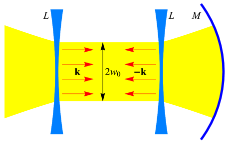
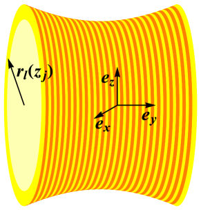
Figure 1: (a) Two lenses ($L$) refract the LG beam (yellow region). The mirror ($M$) reflects the beam, and two counter-propagating beams result. An almost uniform beam waist $w_{0}$ between the lenses, and a series of ring optical potentials with zero amplitude at the center are stacked perpendicular to the beam axis. The wave vectors of the incident and reflected beams are $\pm{\bf k}$. (b) Blowup of the region between the two mirrors where the LG beam forms the ring shaped potential wells. Yellow and orange denote potential minima and maxima. $\mathbf{e}_{x}$, $\mathbf{e}_{y}$ and $\mathbf{e}_{z}$ are unit vectors parallel to the $x$, $y$ and $z$-axes, and $(r_{l}(z_{j}),z_{j})$ are minima of the potential energy.

QR Bound States in LG Rings: The QR Hamiltonian operator in cylindrical coordinates is

$$H=-\frac{\hbar^{2}}{2M}\left(\frac{\partial^{2}}{\partial r^{2}}+\frac{1}{r}\frac{\partial}{\partial r}+\frac{1}{r^{2}}\frac{\partial^{2}}{\partial\phi^{2}}+\frac{\partial^{2}}{\partial z^{2}}\right)+V\left(r,\phi,z\right),$$ (4)

where the first term is the atom kinetic energy in polar coordinates and $V(r,\phi,z)$ is the optical potential resulting from the LG beams, which is calculated as a second-order ac Stark shift SOI-EuroPhysJ-13 and is given in terms of the ac polarizability $\alpha(\omega)$ by $V({\bf r})=-\alpha(\omega)|{\bf E}^{\mathrm{cp}}_{\alpha,l,p}({\bf r},t)|^{2}$. In the standing wave configuration in the nearly constant beam waist region, the optical potential can be taken to be two-dimensional since the width of the rings are very small. For a ${\rm{LG}}_{0}^{l}$ mode ($p=0$ and $l\neq 0$), the potential is independent of $\phi$,

$$V(r,z)=-V_{0}~{}\cos^{2}\big{(}k(z-z_{0})\big{)}~{}\frac{\rho^{2|l|}(z)}{\mathfrak{w}^{2}(z)}e^{-|l|(\rho^{2}(z)-1)},$$ (5)

where $\rho(z)=r/r_{l}(z)$ and $\mathfrak{w}(z)=w(z)/w_{0}$. Potential (5) has a minimum at

$$z=z_{j}\equiv\frac{\pi}{k}j+z_{0},\quad r=r_{l}(z_{j})\equiv w(z_{j})\sqrt{|l|/2},$$ (6)

where $j$ is integer. The trapped atoms execute circular motion around the $z$ axis, i.e., they are QRs. $V(r_{l}(z_{j}),z_{j})$ is given by $V\big{(}r_{l}(z_{j}),z_{j}\big{)}=-V_{0}~{}\big{(}w_{0}/w(z_{j})\big{)}^{2}$. For $z$ close to $z_{j}$,

$$V(r,z)\approx V_{l}(r)+W_{j}(z),$$ (7)

where

$$V_{l}(r)=V(r,z_{j}),\quad W_{j}(z)=\frac{V_{0}k^{2}}{\mathfrak{w}^{2}(z_{j})}~{}(z-z_{j})^{2}.$$ (8)

$W_{j}(z)$ is a harmonic potential in $z-z_{j}$. The corresponding harmonic frequency and length are

$$\omega_{z}(z_{j})={\frac{2}{\mathfrak{w}(z_{j})}\frac{\sqrt{{\mathcal{E}}_{0}V_{0}}}{\hbar},\quad b_{z}(z_{j})=\frac{\sqrt{\mathfrak{w}(z_{j})}}{k}}\bigg{(}\frac{{\mathcal{E}}_{0}}{V_{0}}\bigg{)}^{1/4},$$ (9)

where ${\mathcal{E}}_{0}=\hbar^{2}k^{2}/(2M)$ is the recoil energy.

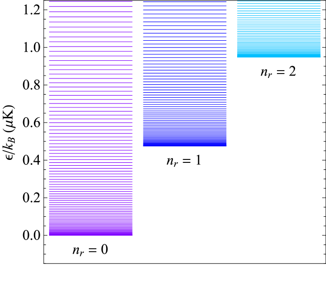
Figure 2: Energies $\epsilon(n_{z},n_{r},m_{\ell})$ of the QR (relative to the QR ground state energy) trapped in an LG beam with $w_{0}=10~{}\mu$m, $l=5$, $p=0$, and $V_{0}=10~{}{\mathcal{E}}_{0}$, where ${\mathcal{E}}_{0}$ is the recoil energy. This gives $r_{l}\equiv r_{l}(z_{j})$ with $j=0$ equal to $15.81~{}\mu$m. Energies with $n_{r}=0$ are shown as purple lines, $n_{r}=1$ as blue lines and $n_{r}=2$ as sky-blue lines. Quantum states with $n_{z}\geq 1$ have very high energies and fall out of the scale of the figure, hence only $n_{z}=0$ are shown.

The optical potential (5) is invariant with respect to rotations about the $z$ axis, therefore the quantum states of the QR in the harmonic approximation (7) are parametrized by radial and vertical quantum numbers $n_{r}$ and $n_{z}$ describing radial and $z$ motion ($n_{r},n_{z}=0,1,2,\ldots$), the orbital momentum quantum number $m_{\ell}$ and projection $m_{F}$ of the hyperfine orbital momentum ${\bf F}$ on the $z$ axis. The ground state has $n_{z}=n_{r}=m_{\ell}=0$, and is $2F+1$ fold degenerate. Orbitally excited states with $m_{\ell}\neq 0$ are $2(2F+1)$ fold degenerate, and have angular momentum $\pm m_{\ell}$. Radial and vertical excitations have $n_{r}\neq 0$ and $n_{z}\neq 0$ respectively. For simplicity, in this paragraph, let us consider an atom trapped at the $z_{0}$ site (i.e., near $z_{j}$ with $j=0$). The QR wave functions and eigen-energies satisy the Schrödinger equation,

$$\Big{[}-\frac{\hbar^{2}}{2M}~{}\nabla^{2}+V(r,z)-\epsilon_{\bf n}\Big{]}\Psi_{\bf n}(\mathbf{r})=0,$$ (10)

where $\mathbf{n}=(n_{z},n_{r},m_{\ell})$. The wave function can be written in cylindrical coordinates $\mathbf{r}=(r,\phi,z)$ as

$$\Psi_{\mathbf{n}}(\mathbf{r})=\frac{1}{\sqrt{2\pi}}~{}\eta_{n_{z}}(z)\psi_{n_{r},m_{\ell}}(r)e^{im\phi},$$ (11)

where $\eta_{n_{z}}(z)$ and $\psi_{n_{r},m_{\ell}}(r)$ satisfy the equations,

$$\Big{[}-\frac{\hbar^{2}}{2M}~{}\frac{d^{2}}{dr^{2}}+W_{0}(z)-\epsilon_{z}(n_{z})\Big{]}\eta_{n_{z}}(z)=0\,,$$ (12)

$$\Big{[}-\frac{\hbar^{2}}{2Mr}~{}\frac{d}{dr}\bigg{(}r~{}\frac{d}{dr}\bigg{)}+V_{l}(r)+m_{\ell}^{2}~{}C(r)-\epsilon_{r}(n_{r},m_{\ell})\Big{]}~{}\psi_{n_{r},m_{\ell}}(r)=0.$$ (13)

$V_{l}(r)$ and $W_{j}(z)$ are given by Eq. (8), and $C(r)=\frac{\hbar^{2}}{2Mr^{2}}$ is the rotational energy of the QR around the $z$ axis. The eigen-energy of the trapped atom is

$$\epsilon(\mathbf{n}) = \epsilon_{z}(n_{z})+\epsilon_{r}(n_{r},m_{\ell}),$$ (14)

where $r_{l}\equiv r_{l}(z_{j})$ with $j=0$. The QR vertical, radial and orbital excitation energies are

$$\varepsilon_{z} = \epsilon_{z}(1)-\epsilon_{z}(0)~{}\approx~{}\hbar\omega_{z},$$

$$\varepsilon_{r} = \epsilon_{r}(1,0)-\epsilon_{r}(0,0),$$

$$\varepsilon_{\ell} = \epsilon_{r}(0,1)-\epsilon_{r}(0,0)~{}\approx~{}C(r_{l}).$$

We assume they satisfy the inequalities,

$$\varepsilon_{z}~{}\gg~{}\varepsilon_{r}~{}\gg~{}\varepsilon_{\ell},$$ (15)

i.e., the orbital excitations are the lowest-energy excitations, whereas the radial and longitudinal excitations have relatively high energies. The energies $\epsilon(n_{z}=0,n_{r},m_{\ell})$, Eq. (14), are shown in Fig. 2. For $l=5$, $w_{0}=10~{}\mu$m, $r_{l}=15.81~{}\mu$m and $V_{0}=10~{}{\mathcal{E}}_{0}=k_{B}\times 35.36~{}\mu$K, the excitation energies are $C(r_{l})=k_{B}\times 0.1613$ nK, $\hbar\omega_{r}=k_{B}\times 0.4776~{}\mu$K and $\hbar\omega_{z}=k_{B}\times 22.36~{}\mu$K, so the inequalities (15) are valid. Quantum states with $n_{z}\geq 1$ have high energies and are not shown in Fig. 2.

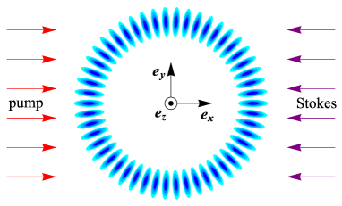
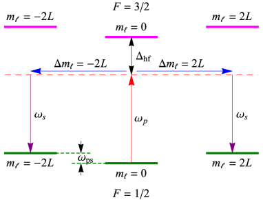
Figure 3: (a) Pump and Stokes radio-frequency pulses (red and purple arrows) and optical rotational counter-propagating LG rotational-kick-pulses with $L=25$ along the $z$ axis. The blue regions indicate the depth of the rotational-kick optical pulse potential. $\mathbf{e}_{x}$, $\mathbf{e}_{y}$ and $\mathbf{e}_{z}$ are unit vectors along the $x$-, $y$- and $z$-axes. (b) Quantum transitions due to the pump, Stokes and rotational-kick pulses (red, purple and blue arrows). The frequencies of the pump and Stokes pulses are $\omega_{p}$ and $\omega_{s}$, and their difference $\omega_{ps}=\omega_{p}-\omega_{s}$ is equal to the transition frequency $\omega_{2L,0}$. Detuning of $\omega_{p}$ from the resonant frequency of the ²S${}_{1/2}(F=1/2)$ to ²S${}_{1/2}(F=3/2)$ quantum transition is $\Delta_{\mathrm{hf}}$.

Rabi Oscillation Method with Raman Pulses: In order to measure the excitation energies of the QR atoms with quantum numbers $n_{r}$, $m_{\ell}$ and $m_{F}$, we propose to subject the QRs to three pulses, as shown in Fig. 3: pump and Stokes radio-frequency pulses with frequencies $\omega_{p}\gtrapprox\omega_{s}$ that are detuned from the quantum transition between the hyperfine states of the ground state, and a LG pulse with frequency $\omega_{e}$ far-detuned from the resonant frequency of the ²S${}_{1/2}\rightarrow{}^{2}$P_3/2 electronic transition. The radio-frequency pump and Stokes light cannot change the orbital quantum number $m_{\ell}$. Therefore we use a LG pulse that allows quantum transitions $|m_{\ell}\rangle\to|m^{\prime}_{\ell}\rangle$ between quantum states with different orbital quantum numbers $m_{\ell}$ and $m^{\prime}_{\ell}$ [see Fig. 3]. The pump and Stokes pulses propagate parallel and anti-parallel to the $x$-axis and are linearly polarized with magnetic field along the $z$ axis (see the supplemental materials (SM) SM ). The pump and Stokes magnetic fields are given by $\mathbf{B}_{\mu}(\mathbf{r},t)=\mathbf{B}_{\mu}^{(0)}~{}\cos(k_{\mu}x-i\omega_{\mu}t)\Theta(t)\Theta(\tau-t)\approx\mathbf{B}_{\mu}^{(0)}\cos(\omega_{\mu}t)\Theta(t)\Theta(\tau-t)$, where $\mu=p,s$ (pump and Stokes beams) and we have assumed square pulses, hence the presence of the $\Theta$ functions. Here we take into account that the wavelengths $\lambda_{\mu}$ are much longer than the radius $r_{l}$ of the QR, hence $\mathbf{B}_{\mu}$ depends on $t$, but not on $\mathbf{r}$, and therefore these pulses do not possess Raman transitions between the quantum states $|n_{r},m_{\ell}\rangle$ and $|n^{\prime}_{r},m^{\prime}_{\ell}\rangle$ and we can approximate $\mathbf{B}_{\mu}(\mathbf{r},t)$ by $\mathbf{B}_{\mu}(t)\equiv\mathbf{B}_{\mu}(0,t)$. Hence, the dipole magnetic interaction between the QR and the radio waves, $H_{\mu}=-g_{F}\mu_{B}\mathbf{F}\cdot\mathbf{B}_{\mu}(t)$, does not depend on $\mathbf{r}$ (the position of the atom), and therefore $\langle n_{r},m_{\ell}|H_{\mu}|n^{\prime}_{r},m^{\prime}_{\ell}\rangle\propto\delta_{n_{r},n^{\prime}_{r}}\delta_{m_{\ell},m^{\prime}_{\ell}}$. For Raman transitions $|n_{r},m_{\ell}\rangle\to|n_{r},m^{\prime}_{\ell}\rangle$ with $m_{\ell}\neq m^{\prime}_{\ell}$, an optical square pulse which breaks the cylindrical symmetry of the QR is required. The electric field of the optical pulse is ${\bf E}_{e}(\mathbf{r},t)=\frac{1}{2}(u_{L,0}(\mathbf{r})+u_{-L,0}(\mathbf{r}))~{}\cos(k_{e}z)~{}\Theta(t)\Theta(\tau-t)~{}e^{-i\omega_{e}t}~{}\mathbf{e}_{x}+{\mathrm{c.c.}}$, where $k_{e}=\omega_{e}/c$ is the wavenumber of the optical pulse and $u_{L,0}(\mathbf{r})$ is given by Eq. (2). We choose the waist radii of the LG pulse $w_{e}$ and the LG beam waist $w_{0}$, and their orbital angular momentums $L$ and $l$ in such a way that $w_{e}\sqrt{|L|/2}=w_{0}\sqrt{|l|/2}$.

The stimulated Raman process corresponding to absorption of a pump photon and stimulated emission of a Stokes photon gives rise to excitation of the QR. This scattering is described by the time-dependent Hamiltonian with matrix elements given by

$${\mathcal{H}}_{n_{r},m_{\ell};n^{\prime}_{r},m^{\prime}_{\ell}}(t)=-2{\mathcal{V}}\cos(\omega_{ps}t)\Theta(t)\Theta(\tau-t)\delta_{n_{r},n^{\prime}_{r}}\sum_{m=\pm 2L}\delta_{m_{\ell},m^{\prime}_{\ell}+m},$$ (16)

where $\omega_{ps}=\omega_{p}-\omega_{s}$ is the difference of frequencies of the pump and Stokes pulses, and

$${\mathcal{V}}=\frac{{\mathcal{V}}_{e}{\mathcal{V}}_{b}}{\hbar\Delta_{\mathrm{hf}}},\ \ {\mathcal{V}}_{b}=\frac{g^{2}\mu_{B}^{2}B_{p}^{(0)}B_{s}^{(0)}}{3\hbar\Delta_{\mathrm{hf}}},\ \ {\mathcal{V}}_{e}=\frac{4\alpha(\omega_{e})}{\pi L!}~{}\frac{P_{e}L^{L}e^{-L}}{w_{e}^{2}c},$$ (17)

$P_{e}$ and $w_{e}$ are the power and the beam waist of the optical pulse, $B_{p}^{(0)}$ and $B_{s}^{(0)}$ are the magnetic field strengths of the pump and Stokes radio-frequency pulses. The subscript $e$ symbolizes the electric dipole interaction of the atom with the optical pulse, and the subscript $b$ symbolizes the magnetic dipole interaction of the atoms with the pump and Stokes radio-frequency pulses. The detuning $\Delta_{\mathrm{hf}}$ of the pump pulse frequency from the ²S${}_{1/2}(F=1/2)\to{}^{2}$S${}_{1/2}(F=1/2)$ quantum transition frequency greatly exceeds the frequency $\omega_{2L,0}$ of the $|0\rangle\to|2L\rangle$ quantum transition,

$$\Delta_{\mathrm{hf}}~{}\gg~{}\omega_{2L,0},$$ (18)

hence we can assume that $\omega_{p}$ and $\omega_{s}$ have the same detuning $\Delta_{\mathrm{hf}}$ from resonance. Details of the Raman scattering of the pump and Stokes light, the Rabi oscillations with Raman pulses used to measure the energy differences of the QR states are presented Ref. Kuzmenko_19 and also in the SM SM .

Consider the QR initially in the ground state $|0\rangle$ subjected to Raman pulses of duration $\tau$ and generalized Rabi frequency $\Omega_{R}=2\sqrt{2}{\mathcal{V}}/\hbar$, such that $\Omega_{R}\tau\approx\pi$. In the 3-level rotating wave approximation rotating-wave-approx-PRL-2007 , the temporal evolution of a single QR wave function is given by $|\Psi(\tau)\rangle=e^{-i{\mathcal{H}}_{R}\tau/\hbar}|0\rangle$, where ${\mathcal{H}}_{R}$ is the Hamiltonian (see SM SM ),

$${\mathcal{H}}_{R} = \hbar\left(\begin{array}[]{ccc}0&\Omega_{R}\sqrt{2}/4&\Omega_{R}\sqrt{2}/4\\ \Omega_{R}\sqrt{2}/4&-\delta&0\\ \Omega_{R}\sqrt{2}/4&0&-\delta\end{array}\right),$$ (22)

$\delta=\omega_{ps}-\omega_{2L,0}$, and the basis vectors are,

$$|0\rangle=\left(\begin{array}[]{c}1\\ 0\\ 0\end{array}\right),\quad|2L\rangle=\left(\begin{array}[]{c}0\\ 1\\ 0\end{array}\right),\quad|-2L\rangle=\left(\begin{array}[]{c}0\\ 0\\ 1\end{array}\right).$$

The probability of finding the quantum rotor in the final state $|f\rangle=2^{-1/2}(|2L\rangle+|-2L\rangle)$ is

$$P_{0}(\delta,\Omega_{R})=\big{|}\langle f|\Psi(\tau)\rangle\big{|}^{2}=\frac{\Omega_{R}^{2}}{\Omega_{R}^{2}+\delta^{2}}\sin^{2}\bigg{(}\frac{\tau}{2}\sqrt{\Omega_{R}^{2}+\delta^{2}}\bigg{)}.$$ (23)

$P_{0}(\delta,\Omega_{R})$ has a peak, $P_{0}(0,\Omega_{R})=1$ at $\delta=0$. The peak width at half maximum is $1.597~{}\Omega_{R}$.

When we have $N=2j_{\max}+1$ atoms singly occupying the sites with $|j|\leq j_{\max}$, the detuning of $\omega_{ps}$ from the resonant frequency of the $j$-th quantum rotor is $\delta_{j}=\delta+4L^{2}j^{2}\big{(}\omega_{0}(r_{l}(0))-\omega_{0}(r_{l}(z_{j}))\big{)}$, where $\delta$ is the detuning of $\omega_{ps}$ from the resonant frequency of the $j=0$ QR, $\omega_{0}(r_{l}(z))=\hbar/(2Mr_{l}^{2}(z_{j}))$ and $r_{l}(z_{j})$ is the radius of the classical circular trajectory. As a result, the peak in the probability to find a QR in the final state is shifted and broadened. The probability to find a QR in the final state is

$$P(\delta,\Omega_{R}) = \frac{1}{2j_{\max}+1}\sum_{j=-j_{\max}}^{j_{\max}}P_{0}\big{(}\delta_{j},\Omega_{R}\big{)}.$$ (24)

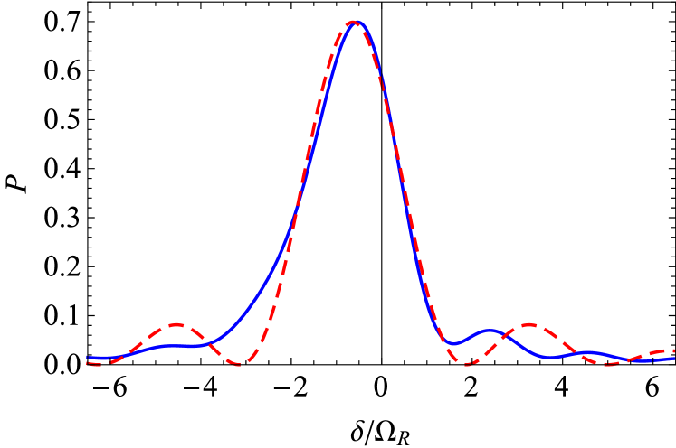
Figure 4: The probability $P$ in Eq. (24) for absorption of a pump photon and stimulated reemission of a Stokes photon with QRs quantum transition from state $|m_{\ell}=0\rangle$ to $|m^{\prime}_{\ell}=50\rangle$ as a function of the difference $\omega_{ps}=\omega_{p}-\omega_{s}$ of the pump and Stokes frequencies $\omega_{p}$ and $\omega_{s}$ (solid blue curve). The dashed red curve shows the fit of $P(\delta,\Omega_{R})$ obtained as explained in the text.

Figure 4 shows $P(\delta,\Omega_{R})$ of Eq. (24) plotted as a function of $\delta$, for $\omega_{0}=21.13$ s^-1, which corresponds to a LG beam with $w_{0}=10~{}\mu$m and $l=25$, Rabi frequency $\Omega_{R}=3.142$ s^-1, pulse duration $\tau\approx\pi/\Omega_{R}=1$ s, $j_{\max}=80$, $m_{\ell}=0$ and $m^{\prime}_{\ell}=50$. The solid blue curve shows that $P(\delta,\Omega_{R})$ has a peak, $P_{\max}=P(\delta_{\max},\Omega_{R})=0.6989$, at $\delta_{\max}=-0.5374\Omega_{R}$. The dashed red curve shows the fitting of $P(\delta,\Omega_{R})$ by the function $P(\delta,\Omega_{R})\approx{\mathcal{A}}\,P_{0}(\delta-\delta_{0},\tilde{\Omega}_{R})$ with ${\mathcal{A}}=0.67987$ and $P_{0}$ is given by Eq. (23) with $\delta_{0}=-0.64002~{}\Omega_{R}$, $\tilde{\Omega}_{R}=1.4865~{}\Omega_{R}$. Note that $\delta_{\max}\neq\delta_{0}$. This is partly because the function $P(\delta,\Omega_{R})$ is not symmetric with respect to the inversion $\delta-\delta_{\max}\to-(\delta-\delta_{\max})$, whereas the function $P_{0}(\delta,\Omega_{R})=P_{0}(-\delta,\Omega_{R})$ is symmetric.

We now show that ground-state QRs in an LG beam can serve as extremely accurate rotation sensors.

Rotation Sensor: Consider a QR in a non-inertial frame rotating with angular velocity $\bm{\Omega}=\Omega~{}\mathbf{e}_{z}$ (see Fig. 2 in the SM SM ). The additional term needed in the Hamiltonian is

$$H_{\Omega}=\hbar\Omega\ell_{z},$$ (25)

where $\ell_{z}=-i\partial_{\phi}$ is the orbital momentum operator. The Hamiltonian (25) lifts the symmetry under the transformation $(x,y,z)\to(-x,y,z)$ but not the rotational symmetry about the $z$-axis. As a result, $m_{\ell}$, the eigenvalue of $\ell_{z}$, is a good quantum number, and the energy levels $\epsilon_{m_{\ell}}$ of the rotational motion become $\epsilon_{m_{\ell}}(\Omega)=\epsilon_{m_{\ell}}+\hbar\Omega\,m_{\ell}$. Hereafter we use the inequalities (15) and restrict ourselves by considering the quantum states with $n_{z}=n_{r}=0$. Moreover, using the inequalities (15), we approximate the rotational energies as $\epsilon_{m_{\ell}}=m_{\ell}^{2}C(r_{l})$, where $r_{l}$ is given by Eq. (6).

Let us consider the frequencies of the quantum transitions between the quantum states $|m_{\ell}\rangle$ and $|m^{\prime}_{\ell}\rangle$ with $m_{\ell}=0,\pm 1$ and $m^{\prime}_{\ell}=m_{\ell}\pm 2L$. We have six spectral lines with frequencies $\omega_{m_{\ell},m_{\ell}\pm 2L}(\Omega)$ which are convenient to order as follows: $\omega_{0,\pm 2L}(\Omega)$, $\omega_{\pm 1,\pm(1+2L)}(\Omega)$, and $\omega_{\pm 1,\pm(1-2L)}(\Omega)$. The frequencies of the quantum transitions between $|\zeta m_{\ell}\rangle$ and $|\zeta m_{\ell}+2\zeta L\rangle$ are

$$\omega_{m_{\ell},m_{\ell}+2\zeta L}(\Omega)=4L\big{(}L+m_{\ell}\big{)}\omega_{0}+2\zeta L\Omega.$$ (26)

where $\zeta=\pm 1$, and the rotational frequency is

$$\omega_{0}=C(r_{l})/\hbar.$$ (27)

Hence, when $\Omega=0$, $\omega_{m_{\ell},m_{\ell}+2L}(0)=\omega_{-m_{\ell},-(m_{\ell}+2L)}(0)$. One can measure the three spectral lines $\omega_{0,2L}(0)=\omega_{0,-2L}(0)$, $\omega_{1,1-2L}(0)=\omega_{-1,-1+2L}(0)$, and $\omega_{1,1+2L}(0)=\omega_{0,-1-2L}(0)$. When $\Omega\neq 0$, the degeneracy of the spectral lines is lifted and the splitting is

$$\Delta\omega_{m_{\ell},m_{\ell}+2L}\equiv\omega_{m_{\ell},m_{\ell}+2L}(\Omega)-\omega_{-m_{\ell},-m_{\ell}-2L}(\Omega)=4L\Omega.$$ (28)

Eq. (28) shows that measuring the splitting of the spectral lines (26), can be used to determine $\Omega$. Figure 5 shows the transition frequencies of the $|m_{\ell}\rangle\to|m_{\ell}\pm 50\rangle$ transitions as functions of $\Omega$. The frequency splitting (28) due to $\Omega$ distinguishes between clockwise and counter-clockwise rotations. All the spectral lines have the same splittings. Hence, the frequencies satisfy the periodic condition,

$$\omega_{m_{\ell}+m_{\Omega},m_{\ell}+m_{\Omega}+2L}\big{(}\Omega-2m_{\Omega}\omega_{0}\big{)}~{}=~{}\omega_{m_{\ell},m_{\ell}+2L}\big{(}\Omega\big{)},$$

where $m_{\Omega}$ is integer.

Figure 5: The frequencies (26) of the quantum transitions $|m_{\ell}\rangle\to|m_{\ell}\pm 50\rangle$ versus the magnitude of the rotational velocity $\Omega$. $\omega_{0}$ is given by Eq. (27).

Rotation measurement accuracy estimate: Note that Eq. (28) does not contain any information regarding the optical potential, the laser frequency or the intensity. Therefore the uncertainty of $\Omega$, $\delta\Omega$, is determined solely by uncertainty $\delta\omega$ of the pump and Stokes frequencies,

$$\delta\Omega = \frac{1}{\sqrt{N}}\,\frac{\delta\omega}{4L}.$$ (29)

Here $N=2j_{\max}+1$ is the number of atoms singly occupying the sites with $|j|\leq j_{\max}$, $\delta\omega=\delta\omega_{p}+\delta\omega_{s}$, and $\delta\omega_{p}$ and $\delta\omega_{s}$ are the uncertainties of the pump and Stokes frequencies. For ⁶Li atoms, we take $\omega_{p}~{}\gtrapprox~{}\omega_{s}~{}\approx~{}1.43\times 10^{9}~{}{\text{s}}^{-1}$. $\delta\omega$ can be estimated as $\delta\omega=2\times 10^{-18}\omega_{p}\approx 2.86\times 10^{-9}~{}{\text{s}}^{-1}$. From Eq. (29) we see that the larger $L$, the smaller is $\delta\Omega$; when $L=25$ and $j_{\max}=80$, $\delta\Omega=2.25\times 10^{-12}$ s^-1.

In order to measure angular velocity when gravity $\mathbf{g}$ is present, place the QRs in the plane perpendicular to $\mathbf{g}$ (let us call this the $x$-$y$ plane), in order to measure the component of the angular velocity in the $z$ direction. If an additional acceleration $\mathbf{a}$ in the $x$-$y$ plane is present, there is an additional splitting of the QR ground state degeneracy due to the acceleration, and the frequency splitting in Eq. (28) becomes dependent on $m_{\ell}$. Hence, turn the plane of the QRs to be perpendicular to ${\mathbf{g}}^{\prime}=\mathbf{g}-\mathbf{a}$ so that the frequency splitting (28) is independent on $m_{\ell}$, and obtain the energy splitting of the levels caused just by $\Omega^{\prime}=\bm{\Omega}\cdot\mathbf{e}^{\prime}_{z}$, where $\mathbf{e}^{\prime}_{z}$ is the unit vector along $-\mathbf{g}^{\prime}$. For details see the SM SM .

Summary and Conclusion: Cold atoms trapped in a Laguerre-Gauss optical potential (5) are confined to circular rings (donuts) of radius $r_{l}$ with centers on the axis of the Laguerre-Gauss beam. Rings with one atom per site (to suppress spin-exchange collisions) can be used as high-accuracy rotation sensors. When $r_{l}=15.81~{}\mu$m, the accuracy obtained with $N=161$ atoms singly occupying the sites with $|j|\leq 80$ is $\delta\Omega=2.25\times 10^{-12}$ s^-1. This is better than the accuracy $\delta\Omega=6.4\times 10^{-10}$ s^-1 reported in Ref. Kuzmenko_19 . Moreover, the rotation sensor accuracy is much better than $\delta\Omega_{\mathrm{NIST}}=3\times 10^{-8}$ s^-1 reported in Ref. rotation-sensor-NIST-2016 .

The rings between the lenses in Fig. 1 have slightly different radii [see Eq. (6)]. As a result, different transition frequencies are obtained from of the $m_{\ell}\to m^{\prime}_{\ell}$ transition for different $z_{j}$: $\omega_{m_{\ell},m^{\prime}_{\ell}}(z_{j})=\omega_{m_{\ell},m^{\prime}_{\ell}}(0)C(r_{l}(z_{j}))/C(r_{l}(0))$. Hence, the width of the Rabi oscillation is broadened. For example, when $\omega_{0}=21.13$ s^-1, $\Omega_{R}=3.142$ s^-1, and there are $N=161$ singly occupied sites with $|j|\leq 80$, the resulting effective width of the Rabi oscillation peak is $\tilde{\Omega}_{R}=1.4865~{}\Omega_{R}$ instead of $\Omega_{R}$ for a single QR (see Fig. 4).

References

(1)
I. Kuzmenko, T. Kuzmenko, Y. Avishai and Y. B. Band,
Phys. Rev. A 100, 033415 (2019).
(2)
G. Goubau, and F. Schwering,
IRE Trans. 9, 248 256 (1961).
(3)
L. Allen, et al.,
Phys. Rev. A 45, 8185 (1992).
(4)
M.A. Clifford, J. Arlt, J. Courtial, K. Dholakia,
Optics Communications 156, 300 (1998).
(5) F. Pampaloni, Joerg Enderlein, arXiv:physics/0410021.
(6) W. H. Carter, M. F. Aburdene, J. Opt. Soc. Am. A 4, 1949 (1987).
(7) L. Viverit, C. Menotti, T. Calarco, and A. Smerzi, Phys. Rev. Lett.93, 110401 (2004).
(8) I. Bloch, J. Dalibard, W. Zwerger, Rev. Mod. Phys. 80, 885 (2008).
(9) J. M. Gibbons et al,
Phys. Rev. A 78, 043418 (2008).
(10)
Alternatively, one could consider a different configuration consisting of a red-detuned version of a trap developed by T. Kuga et al.,
Phys. Rev. Lett. 78, 4713 (1997), with a LG beam and two additional ``plugging'' laser beams which limit the atomic motion along the optical axis of the LG beam.
(11) F. Le Kien, P. Schneeweiss and A. Rauschenbeutel,
Eur. Phys. J. D 67, 92 (2013).
(12)
N. F. Ramsey,
Phys. Rev. 78, 695 (1950).
(13)
T. Zanon-Willette et al.,
Phys. Rev. A 90, 053427 (2014).