Globally Optimal Contrast Maximisation for Event-based Motion Estimation

Abstract

Contrast maximisation estimates the motion captured in an event stream by maximising the sharpness of the motion-compensated event image. To carry out contrast maximisation, many previous works employ iterative optimisation algorithms, such as conjugate gradient, which require good initialisation to avoid converging to bad local minima. To alleviate this weakness, we propose a new globally optimal event-based motion estimation algorithm. Based on branch-and-bound (BnB), our method solves rotational (3DoF) motion estimation on event streams, which supports practical applications such as video stabilisation and attitude estimation. Underpinning our method are novel bounding functions for contrast maximisation, whose theoretical validity is rigorously established. We show concrete examples from public datasets where globally optimal solutions are vital to the success of contrast maximisation. Despite its exact nature, our algorithm is currently able to process a $50,000$-event input in $\approx 300$ seconds (a locally optimal solver takes $\approx 30$ seconds on the same input). The potential for GPU acceleration will also be discussed.

1 Introduction

By asynchronously detecting brightness changes, event cameras offer a fundamentally different way to detect and characterise physical motion. Currently, active research is being conducted to employ event cameras in many areas, such as robotics/UAVs [10, 23], autonomous driving[34, 24, 33], and spacecraft navigation [8, 7]. While the utility of event cameras extends beyond motion perception, e.g., object recognition and tracking [28, 30], the focus of our work is on estimating visual motion using event cameras.

Due to the different nature of the data, new approaches are required to extract motion from event streams. A recent successful framework is contrast maximisation (CM) [14]. Given an event stream, CM aims to find the motion parameters that yield the sharpest motion-compensated event image; see Fig. 1. Intuitively, the correct motion parameters will align corresponding events, thereby producing an image with high contrast. We formally define CM below.

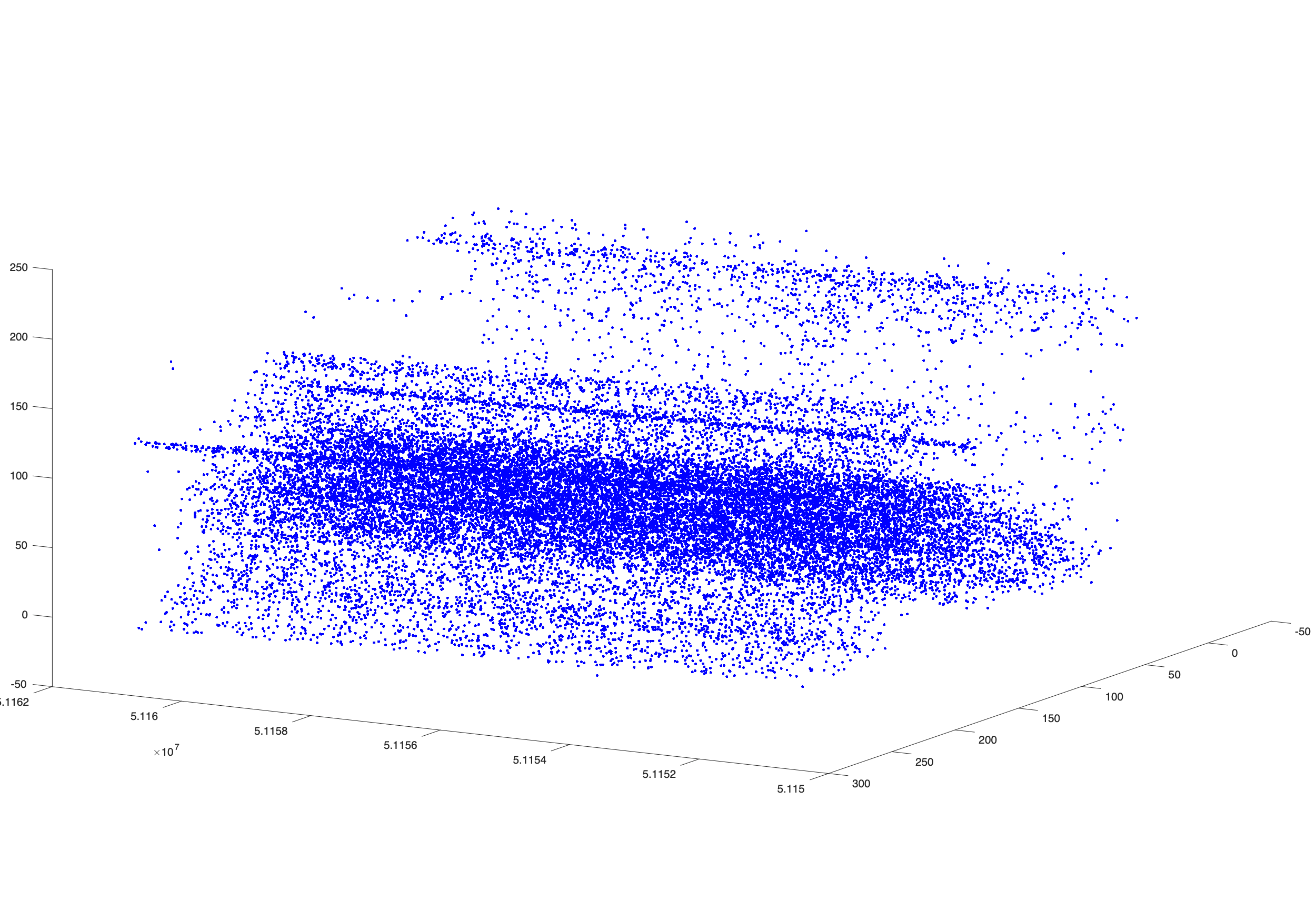
(a) Event stream (w/o polarity).

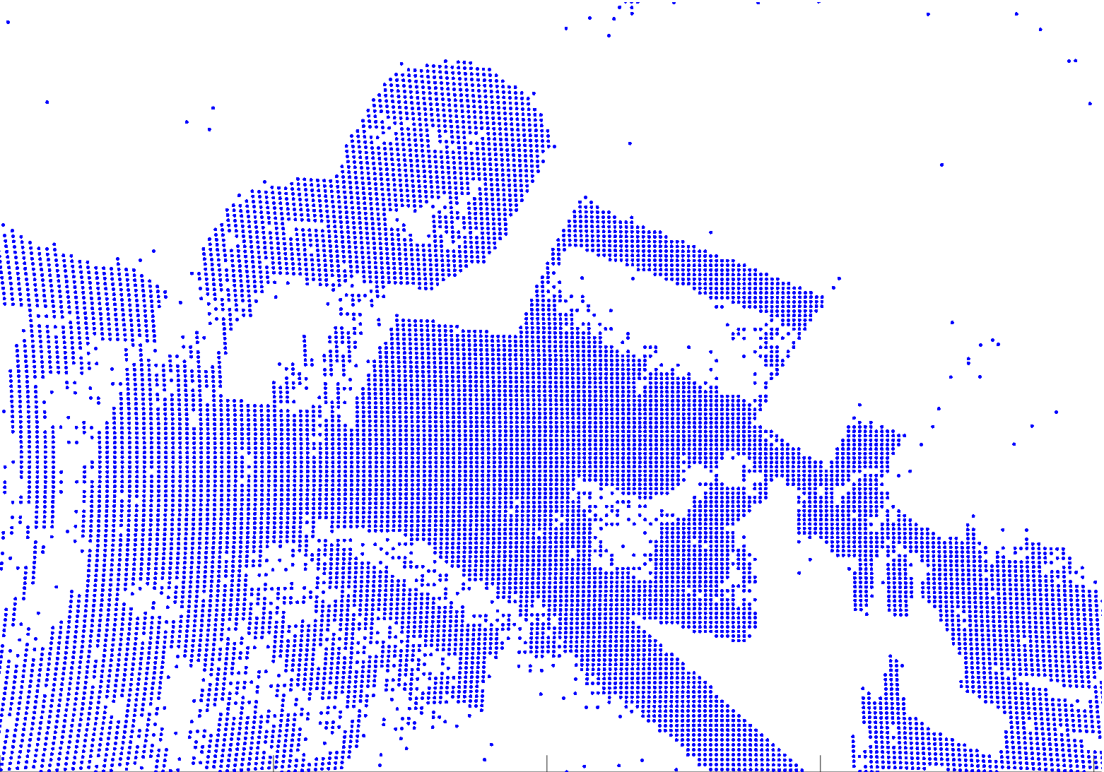
(b) Contrast = $0.9993$ (identity).

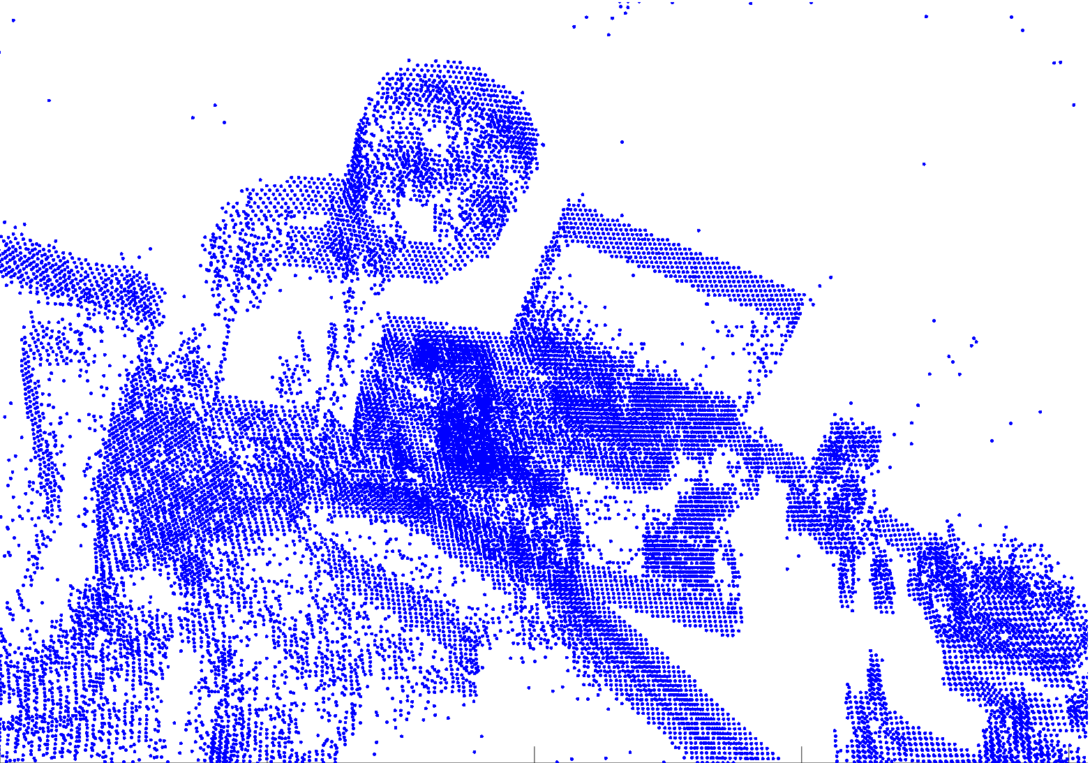
(c) Contrast = $1.0103$ (local).

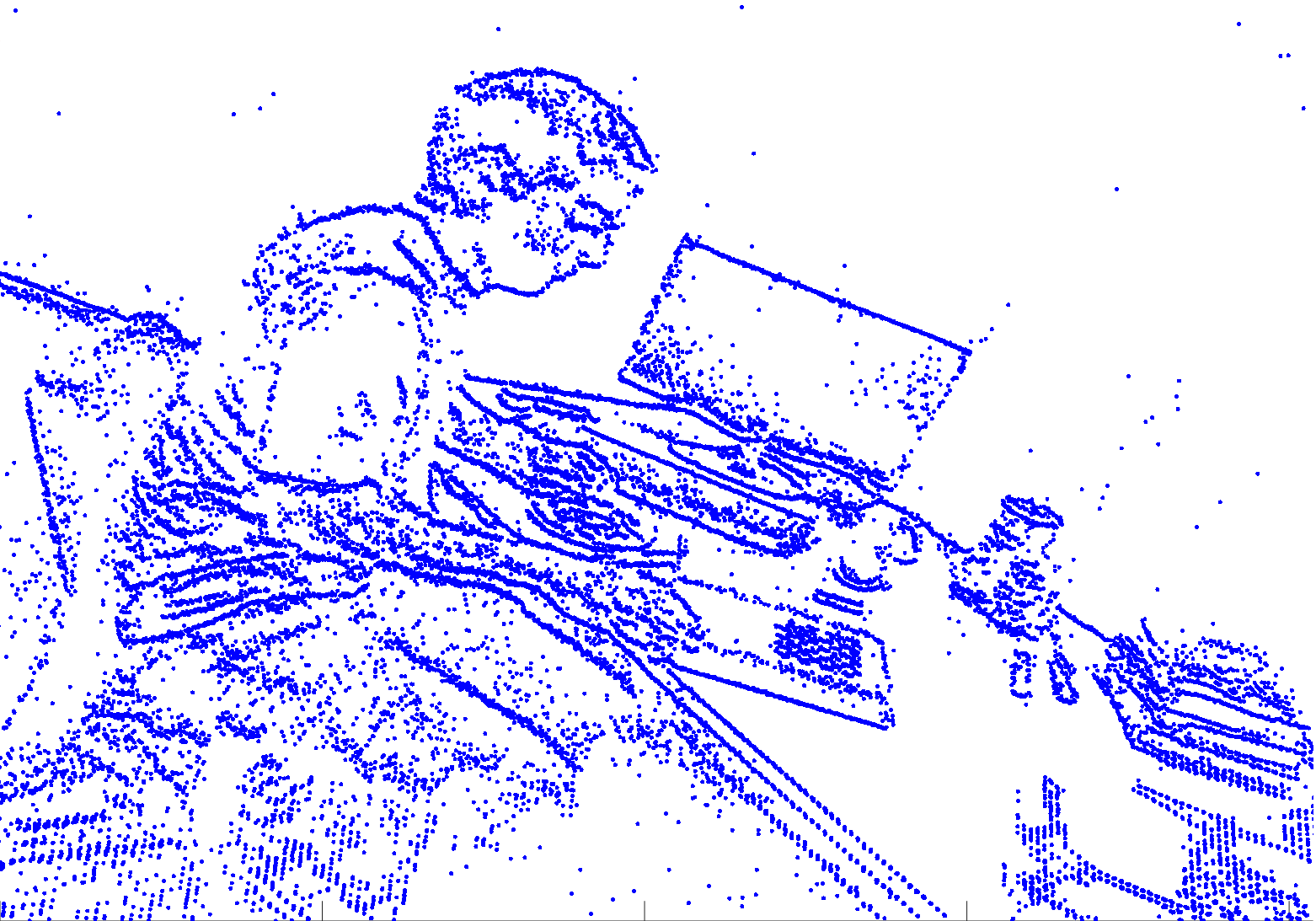
(d) Contrast = $1.9748$ (global).

Figure 1: (a) $10$ ms event stream under rotational motion [15]. Since event polarity is not used in our work, the events are plotted in the same colour. (b) Event image without motion compensation (identity transformation). (c)(d) Event images produced with locally and globally optimal contrast maximisation.

Event image

Let $\mathcal{E}=\{\bm{e}_{i}\}_{i}^{N}$ be an event stream recorded over time duration $\mathcal{T}=[0,t_{\max}]$. Each event $\bm{e}_{i}=(\mathbf{u}_{i},t_{i},p_{i})$ contains an image position $\mathbf{u}_{i}$, time stamp $t_{i}\in\mathcal{T}$, and polarity $p_{i}\in\{-1,+1\}$. We assume $\mathcal{E}$ was produced under camera motion $\mathcal{M}$ over a 3D scene, thus each $\bm{e}_{i}$ is associated with a scene point that triggered the event.

We parameterise $\mathcal{M}$ by a vector $\bm{\omega}\in\Omega$, and let $X=\{\mathbf{x}_{j}\}_{j=1}^{P}$ be the centre coordinates of the pixels in the image plane of the event sensor. Under CM, the event image $H_{c}$ is defined as a function of $\bm{\omega}$, and the intensity at pixel $\mathbf{x}_{j}$ is

$$H_{c}(\mathbf{x}_{j};\bm{\omega})=\sum_{i=1}^{N}\bm{\delta}(\mathbf{x}_{j}-f(\mathbf{u}_{i},t_{i};\,\bm{\omega})),$$ (1)

where $\bm{\delta}$ is a kernel function (e.g., Gaussian). Following [14, Sec. 2.1], we do not use event polarities in (1). $H_{c}$ is regarded to be captured at time $0$, and the function

$$\mathbf{u}^{\prime}_{i}=f(\mathbf{u}_{i},t_{i};\,\bm{\omega})$$ (2)

warps $\mathbf{u}_{i}$ to $\mathbf{u}^{\prime}_{i}$ in $H_{c}$ by “undoing” the motion $\mathcal{M}$ between time $0$ and $t_{i}$. Intuitively, $\mathbf{u}^{\prime}_{i}$ is the image position of the 3D scene point that triggered $\bm{e}_{i}$, if it was observed at time $0$.

In practice, the region of support of the kernel $\bm{\delta}$ in (1) is small w.r.t. image dimensions, e.g., Gaussian kernels with bandwidth $\sigma=1$ pixel were used in [14, Sec. 2]. This motivates the usage of “discrete” event images

$$H_{d}(\mathbf{x}_{j};\bm{\omega})=\sum_{i=1}^{N}\mathbb{I}(f(\mathbf{u}_{i},t_{i};\,\bm{\omega})\leavevmode\nobreak\ \text{lies in pixel}\leavevmode\nobreak\ \mathbf{x}_{j}),$$ (3)

where $\mathbb{I}$ returns $1$ if the input predicate is true, and $0$ otherwise. As we will show later, conducting CM using $H_{c}$ (with small bandwidth) and $H_{d}$ yields almost identical results.

Contrast maximisation

The contrast of an event image $H$ (continuous or discrete) is the variance of its pixel values. Since $H$ depends on $\bm{\omega}$, the contrast is also a function of $\bm{\omega}$

$$C(\bm{\omega})=\dfrac{1}{P}\sum_{j=1}^{P}(H(\mathbf{x}_{j};\bm{\omega})-\mu(\bm{\omega}))^{2},$$ (4)

where $\mu(\bm{\omega})$ is the mean intensity

$$\mu(\bm{\omega})=\dfrac{1}{P}\sum_{j=1}^{P}H(\mathbf{x}_{j};\bm{\omega}).$$ (5)

CM [14] estimates $\mathcal{M}$ by maximising the contrast of $H$, i.e.,

$$\max_{\bm{\omega}\in\Omega}\leavevmode\nobreak\ \leavevmode\nobreak\ C(\bm{\omega}).$$ (6)

The intuition is that the correct $\bm{\omega}$ will allow $\mathcal{M}$ to align events that correspond to the same scene points in $H$, thus leading to a sharp or high-contrast event image; see Fig. 1.

Global versus local solutions

By globally optimal (or “global”) solution to CM (6), we mean $\bm{\omega}^{*}\in\Omega$ such that

$$C(\bm{\omega}^{*})\geq C(\bm{\omega})\;\;\forall\bm{\omega}\in\Omega.$$ (7)

A solution $\hat{\bm{\omega}}$ is approximate if $C(\hat{\bm{\omega}})<C(\bm{\omega}^{*})$. Also, a solution is locally optimal (or “local”) if it is the maximiser of its neighbourhood [26, Chap. 2]. All global solutions are locally optimal, but the converse is not true.

1.1 Previous works

Previous works on CM (e.g., [14, 12, 30, 31]) apply nonlinear optimisation (e.g., conjugate gradient) to solve (6). Given an initial solution $\bm{\omega}^{(0)}$, the solution is successively updated until convergence to a locally optimal solution. In practice, if the local solution is a bad approximate solution, there can be significant differences in its quality compared to the global solution; see Fig. 1. This can occur when $\bm{\omega}^{(0)}$ is too distant from good solutions, or $C(\bm{\omega})$ is too nonconcave (e.g., when $\bm{\delta}$ has a very small bandwidth). Thus, algorithms that can find $\bm{\omega}^{*}$ are desirable.

Recent improvements to CM include modifying the objective function to better suit the targeted settings [12, 31]. However, the optimisation work horse remains locally optimal methods. Other frameworks for event processing [6, 20, 21, 13, 19, 7] conduct filtering, Hough transform, or specialised optimisation schemes; these are generally less flexible than CM [14]. There is also active research in applying deep learning to event data [37, 38, 35, 29], which require a separate training phase on large datasets.

Contributions

We focus on estimating rotational motion from events, which is useful for several applications, e.g., video stabilisation [15] and attitude estimation [8].

Specifically, we propose a BnB method for globally optimal CM for rotation estimation. Unlike previous CM techniques, our algorithm does not require external initialisations $\bm{\omega}^{(0)}$, and can guarantee finding the global solution $\bm{\omega}^{*}$ to (6). Our core contributions are novel bounding functions for CM, whose theoretical validity are established. As we will show in Sec. 4, while local methods generally produce acceptable results [15, 14], they often fail during periods with fast rotational motions. On the other hand, our global method always returns accurate results.

2 Rotation estimation from events

If duration $\mathcal{T}$ is small (e.g., $t_{\max}=10ms$), a fixed axis of rotation and constant angular velocity can be assumed for $\mathcal{M}$ [14]. Following [14, Sec. 3], $\mathcal{M}$ can be parametrised as a $3$-vector $\bm{\omega}$, where the direction of $\bm{\omega}$ is the axis of rotation, and the length $\|\bm{\omega}\|_{2}$ of $\bm{\omega}$ is the angular rate of change. Between time $0$ and $t$, the rotation undergone is

$$\mathbf{R}(t;\bm{\omega})=\text{exp}([\bm{\omega}\,t]_{\times}),$$ (8)

where $\bm{\omega}t$ is the axis-angle representation of the rotation, $[\bm{\omega}t]_{\times}$ is the skew symmetric form of $\bm{\omega}t$, and exp is the exponential map (see [1] for details).

Let $\mathbf{K}$ be the $3\times 3$ intrinsic matrix of the event camera ($\mathbf{K}$ is known after calibration [36, 2]). The warp (2) is thus

$$f(\mathbf{u}_{i},t_{i};\,\bm{\omega})=\frac{\mathbf{K}^{(1:2)}\mathbf{R}(t_{i};\bm{\omega})\tilde{\mathbf{u}}_{i}}{\mathbf{K}^{(3)}\mathbf{R}(t_{i};\bm{\omega})\tilde{\mathbf{u}}_{i}},$$ (9)

where $\tilde{\mathbf{u}}_{i}=[\mathbf{u}_{i}^{T}\leavevmode\nobreak\ 1]^{T}$ is the homogeneous version of $\mathbf{u}_{i}$, and $\mathbf{K}^{(1:2)}$ and $\mathbf{K}^{(3)}$ are respectively the first-two rows and third row of $\mathbf{K}$. Intuitively, (9) rotates the ray that passes through $\mathbf{u}_{i}$ using $\mathbf{R}(t_{i};\bm{\omega})$, then projects the rotated ray onto $H$.

Following [14, Sec. 3], we also assume a known maximum angular rate $r_{\max}$. The domain is thus an $r_{\max}$-ball

$$\Omega=\{\bm{\omega}\in\mathbb{R}^{3}\mid\|\bm{\omega}\|_{2}\leq r_{\max}\},$$ (10)

and our problem reduces to maximising $C(\bm{\omega})$ over this ball, based on the rotational motion model (9).

2.1 Main algorithm

Algorithm 1 summarises our BnB algorithm to achieve globally optimal CM for rotation estimation. Starting from the tightest bounding cube $\mathbb{B}$ on the $r_{\max}$-ball $\Omega$ (the initial $\mathbb{B}$ is thus of size $(2r_{\max})^{3}$), the algorithm recursively subdivides $\mathbb{B}$ and prunes the subcubes until the global solution is found. A lower bound $\underline{C}$ and upper bound $\overline{C}(\mathbb{B})$ are used to prune each $\mathbb{B}$. When the difference between the bounds is smaller than $\tau$, the algorithm terminates with $\hat{\bm{\omega}}$ being the global solution $\bm{\omega}^{*}$ (up to error $\tau$, which can be chosen to be arbitrarily small). See [17, 16] for details of BnB.

As alluded to above, our core contributions are novel and effective bounding functions for CM using BnB. We describe our bounding functions in the next section.

Algorithm 1 BnB for rotation estimation from events.

0:  Event stream $\mathcal{E}=\{\bm{e}_{i}\}^{N}_{i=1}$, maximum angular rate of change $r_{\max}$, convergence threshold $\tau$.

1:  $q\leftarrow$ Initialise priority queue.

2:  $\mathbb{B}\leftarrow$ Cube in $\mathbb{R}^{3}$ of size $(2r_{\max})^{3}$ centred at origin.

3:  $\bm{\omega}_{c}\leftarrow$ Centre of $\mathbb{B}$.

4:  $\hat{\bm{\omega}}\leftarrow\bm{\omega}_{c}$.

5:  Insert $\mathbb{B}$ into $q$ with priority $\overline{C}(\mathbb{B})$.

6:  while $q$ is not empty do

7:     $\mathbb{B}\leftarrow$ Dequeue top item from $q$.

8:     If $\overline{C}(\mathbb{B})-C(\hat{\bm{\omega}})\leq\tau$, then terminate.

9:     $\bm{\omega}_{c}\leftarrow$ Centre of $\mathbb{B}$.

10:     If $C(\bm{\omega}_{c})\geq C(\hat{\bm{\omega}})$, then $\hat{\bm{\omega}}\leftarrow\bm{\omega}_{c}$.

11:     Uniformly subdivide $\mathbb{B}$ into $8$ subcubes $\mathbb{B}_{1},\ldots,\mathbb{B}_{8}$.

12:     for $i=1,\cdots,8$ do

13:        if $\overline{C}(\mathbb{B}_{i})\geq C(\hat{\bm{\omega}})$ then

14:           Insert $\mathbb{B}_{i}$ into $q$ with priority $\overline{C}(\mathbb{B}_{i})$.

15:        end if

16:     end for

17:  end while

18:  return  $\hat{\bm{\omega}}$ as $\bm{\omega}^{*}$.

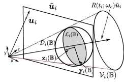
(a)

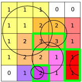
(b)

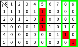
(c)

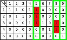
(d)

Figure 2: (a) The vector $R(t_{i},\bm{\omega})\tilde{\mathbf{u}}_{i}$ for all $\bm{\omega}\in\mathbb{B}$ lies in the cone $\mathcal{V}_{i}(\mathbb{B})$, and the projection of $\mathcal{V}_{i}(\mathbb{B})$ onto the image plane is an elliptical region $\mathcal{L}_{i}(\mathbb{B})$. (b) Example with $5\times 5$ pixel image and $N=5$ events; there are thus $N=5$ discs $\{\mathcal{D}_{i}(\mathbb{B})\}_{i=1}^{5}$ on the image. The value in a pixel is the number of discs that intersect the pixel. Pixels with the same color are from the same connected component (CC); there are $9$ CCs in this example. (c)(d) Incidence matrix $\mathbf{M}$ corresponding to the example in (b). The solution of IQP and R-IQP are indicated respectively in (c) and (d), where entries $(i,k)$ of $\mathbf{Z}$ that are set to $1$ are marked in red. The dominant columns of $\mathbf{M}$ are outlined in green, and their corresponding CCs are also outlined in green in (b).

3 Bounds for contrast maximisation

To search for the maximum of $C(\bm{\omega})$ using BnB, a lower and upper bound on the objective are required.

The lower bound $\underline{C}$ must satisfy the condition

$$\underline{C}\leq\max_{\bm{\omega}\in\Omega}\leavevmode\nobreak\ C(\bm{\omega}),$$ (11)

which is trivially achieved by any (suboptimal) solution. In Algorithm 1, the current best solution $\hat{\bm{\omega}}$ is used to provide $\underline{C}$, which is iteratively raised as the search progresses.

The upper bound $\overline{C}(\mathbb{B})$ is defined over a region (a subcube) $\mathbb{B}$ of $\Omega$, and must satisfy the condition

$$\overline{C}(\mathbb{B})\geq\max_{\bm{\omega}\in\mathbb{B}}\leavevmode\nobreak\ C(\bm{\omega}).$$ (A1)

Also, as $\mathbb{B}$ collapses to a single point $\bm{\omega}$, $\overline{C}(\mathbb{B})$ should equate to $C(\bm{\omega})$; more formally,

$$\overline{C}(\mathbb{B})\to C(\bm{\omega})\leavevmode\nobreak\ \leavevmode\nobreak\ \text{when}\leavevmode\nobreak\ \leavevmode\nobreak\ \mathbb{B}\to\bm{\omega}.$$ (A2)

See [17] for the rationale of the above conditions for BnB.

Deriving the upper bound is a more involved process. Our starting point is to rewrite (4) as

$$C(\bm{\omega})=\dfrac{1}{P}\sum_{j=1}^{P}H(\mathbf{x}_{j};\bm{\omega})^{2}-\mu(\bm{\omega})^{2},$$ (12)

which motivates a bound based on two components

$$\overline{C}(\mathbb{B}):=\dfrac{1}{P}\overline{S}(\mathbb{B})-\underline{\mu}(\mathbb{B})^{2},$$ (13)

where $\overline{S}(\mathbb{B})$ is an upper bound

$$\overline{S}(\mathbb{B})\geq\max_{\bm{\omega}\in\mathbb{B}}\leavevmode\nobreak\ \sum_{j=1}^{P}H(\mathbf{x}_{j};\bm{\omega})^{2}$$ (14)

on the “sum of squares (SoS)” component, and

$$\underline{\mu}(\mathbb{B})\leq\min_{\bm{\omega}\in\mathbb{B}}\leavevmode\nobreak\ \mu(\bm{\omega})$$ (15)

is a lower bound of the mean pixel value. Given (14) and (15), then (13) satisfies A1. If equality holds in (14) and (15) when $\mathbb{B}$ is singleton, then (13) also satisfies A2.

In Secs. 3.1 and 3.2, we develop $\overline{S}(\mathbb{B})$ for continuous and discrete event images, before deriving $\underline{\mu}(\mathbb{B})$ in Sec. 3.3.

3.1 SoS bound for continuous event image

For the continuous event image $H_{c}$ (1), our SoS upper bound (denoted $\overline{S}_{c}$) is defined as

$$\overline{S}_{c}(\mathbb{B}):=\sum_{j=1}^{P}\overline{H}_{c}(\mathbf{x}_{j};\mathbb{B})^{2},$$ (16)

where $\overline{H}_{c}(\mathbf{x}_{j};\mathbb{B})$ is an upper bound on the value of $H_{c}$ at $\mathbf{x}_{j}$. To obtain $\overline{H}_{c}(\mathbf{x}_{j};\mathbb{B})$, we bound the position

$$\{\mathbf{u}^{\prime}_{i}=f(\mathbf{u}_{i},t_{i};\,\bm{\omega})\mid\bm{\omega}\leavevmode\nobreak\ \in\mathbb{B}\}$$ (17)

of each warped event, under all possible $\bm{\omega}\in\mathbb{B}$ for the warping function (9). To this end, let $\bm{\omega}_{\mathbf{c}}$ be the centre of a cube $\mathbb{B}$, and $\bm{\omega}_{\mathbf{p}}$ and $\bm{\omega}_{\mathbf{q}}$ be opposite corners of $\mathbb{B}$. Define

$$\alpha_{i}(\mathbb{B}):=0.5\|\bm{\omega}_{\mathbf{p}}t_{i}-\bm{\omega}_{\mathbf{q}}t_{i}\|_{2}.$$ (18)

Then, the following inequality can be established

$$\angle(\mathbf{R}(t_{i};\bm{\omega}_{\mathbf{c}})\tilde{\mathbf{u}}_{i},\mathbf{R}(t_{i};\bm{\omega})\tilde{\mathbf{u}}_{i})\leq\alpha_{i}(\mathbb{B}),$$ (19)

which is an extension of  [16, Lemma 3.2]. Intuitively, (19) states that the rotated vector $\mathbf{R}(t_{i};\bm{\omega})\tilde{\mathbf{u}}_{i}$ under all $\bm{\omega}\in\mathbb{B}$ must lie within the cone

$$\mathcal{V}_{i}(\mathbb{B}):=\left\{\tilde{\mathbf{u}}\in\mathbb{R}^{3}\mid\angle(\mathbf{R}(t_{i};\bm{\omega}_{\mathbf{c}})\tilde{\mathbf{u}}_{i},\tilde{\mathbf{u}})\leq\alpha_{i}(\mathbb{B})\right\}.$$ (20)

Fig. 2a illustrates the cone $\mathcal{V}_{i}(\mathbb{B})$. Now, the pinhole projection of all the rays in $\mathcal{V}_{i}(\mathbb{B})$ yields the 2D region

$$\mathcal{L}_{i}(\mathbb{B})=\left\{\mathbf{x}=\frac{\mathbf{K}^{(1:2)}\tilde{\mathbf{u}}}{\mathbf{K}^{(3)}\tilde{\mathbf{u}}}\,\middle|\,\tilde{\mathbf{u}}\in\mathcal{V}_{i}(\mathbb{B})\right\},$$ (21)

which is an elliptical region [25, Chap. 2]; see Fig. 2a. Further, the centre $\mathbf{c}_{i}(\mathbb{B})$, semi-major axis $\mathbf{y}_{i}(\mathbb{B})$ and semi-minor axis $\mathbf{z}_{i}(\mathbb{B})$ of $\mathcal{L}_{i}(\mathbb{B})$ can be analytically determined (see the supplementary material). We further define

$$\mathcal{D}_{i}(\mathbb{B})=\left\{\mathbf{x}\in\mathbb{R}^{2}\,\middle|\,\|\mathbf{x}-\mathbf{c}_{i}(\mathbb{B})\|\leq\|\mathbf{y}_{i}(\mathbb{B})\|\right\},$$ (22)

i.e., the smallest disc that contains $\mathcal{L}_{i}(\mathbb{B})$.

By construction, $\mathcal{D}_{i}(\mathbb{B})$ fully contains the set of positions that $\mathbf{u}_{i}^{\prime}$ can take for all $\bm{\omega}\in\mathbb{B}$, i.e., the set (17). We thus define the upper bound on the pixel values of $H_{c}$ as

$$\overline{H}_{c}(\mathbf{x}_{j};\mathbb{B})=\sum_{i=1}^{N}\bm{\delta}\left(\max\left(\|\mathbf{x}_{j}-\mathbf{c}_{i}(\mathbb{B})\|-\|\mathbf{y}_{i}(\mathbb{B})\|,0\right)\right).$$ (23)

Intuitively, we take the distance of $\mathbf{x}_{j}$ to the boundary of $\mathcal{D}_{i}(\mathbb{B})$ to calculate the intensity, and if $\mathbf{x}_{j}$ is within the disc then the distance is zero.

Lemma 1.

$$\overline{H}_{c}(\mathbf{x}_{j};\mathbb{B})\geq\max_{\bm{\omega}\in\mathbb{B}}\leavevmode\nobreak\ H_{c}(\mathbf{x}_{j};\bm{\omega})$$ (24)

with equality achieved if $\mathbb{B}$ is singleton, i.e., $\mathbb{B}=\{\bm{\omega}\}$.

Proof.

See supplementary material. ∎

Given Lemma 5, it is clear that $\overline{S}_{c}(\mathbb{B})$ satisfies the conditions (see Sec. 3) to be a valid component in the upper bound (13) for the continuous event image $H_{c}$.

3.2 SoS bound for discrete event image

Given the $N$ discs $\{\mathcal{D}_{i}(\mathbb{B})\}^{N}_{i=1}$ associated with the $N$ events, define the intersection matrix $\mathbf{T}\in\{0,1\}^{N\times P}$:

$$\mathbf{T}_{i,j}=\begin{cases}1&\mathcal{D}_{i}(\mathbb{B})\leavevmode\nobreak\ \text{intersects pixel}\leavevmode\nobreak\ \mathbf{x}_{j};\\ 0&\text{otherwise}.\end{cases}$$ (25)

The disc-pixel intersections can be computed efficiently using established techniques [32, 11]. We assume $\sum_{j=1}^{P}\mathbf{T}_{i,j}>0$ for all $i$, i.e., each disc intersects at least one pixel. If there are discs that lie beyond the image plane, we ignore these discs without loss of generality.

A direct extension of $\overline{H}_{c}$ (23) to the discrete case would be to calculate the pixel upper bound value as

$$\overline{H}_{d}(\mathbf{x}_{j};\mathbb{B})=\sum_{i=1}^{N}\mathbf{T}_{i,j},$$ (26)

i.e., number of discs that intersect the pixel; see Fig. 2b. This can however be overly pessimistic, since the pixel value for the discrete event image (3) satisfies

$$\sum_{j=1}^{P}H_{d}(\mathbf{x}_{j};\bm{\omega})\leq N\implies\sum_{j=1}^{P}H_{d}(\mathbf{x}_{j};\bm{\omega})^{2}\leq N^{2},$$ (27)

whereas by using (26),

$$\sum_{j=1}^{P}\overline{H}_{d}(\mathbf{x}_{j};\mathbb{B})\leq PN\implies\sum_{j=1}^{P}\overline{H}_{d}(\mathbf{x}_{j};\bm{\omega})^{2}\leq(PN)^{2}.$$ (28)

Note that $P$ is the number of pixels (e.g., $P=240\times 320=76k$ for IniVation Davis 240C [3]), thus $(PN)^{2}\gg N^{2}$.

To get a tighter bound, we note that the discs $\{\mathcal{D}_{i}(\mathbb{B})\}^{N}_{i=1}$ partition $X$ into a set of connected components (CC)

$$\{\mathcal{G}_{k}\}^{K}_{k=1},$$ (29)

where each $\mathcal{G}_{k}$ is a connected set of pixels that are intersected by the same discs; see Fig. 2b. Then, define the incidence matrix $\mathbf{M}\in\{0,1\}^{N\times K}$, where

$$\mathbf{M}_{i,k}=\begin{cases}1&\exists\mathbf{x}_{j}\in\mathcal{G}_{k}\;\text{such that}\leavevmode\nobreak\ \mathbf{T}_{i,j}=1;\\ 0&\text{otherwise.}\end{cases}$$ (30)

In words, $\mathbf{M}_{i,k}=1$ if $\mathcal{D}_{i}(\mathbb{B})$ is a disc that intersect to form $\mathcal{G}_{k}$. We then formulate the integer quadratic program

$$\begin{aligned} \overline{S}^{*}_{d}(\mathbb{B})=\max_{\mathbf{Z}\in\{0,1\}^{N\times K}}\quad&\sum^{K}_{k=1}\left(\sum_{i=1}^{N}\mathbf{Z}_{i,k}\mathbf{M}_{i,k}\right)^{2}\\ \text{s.t.}\quad&\mathbf{Z}_{i,k}\leq\mathbf{M}_{i,k},\;\;\forall i,k,\\ &\sum_{k=1}^{K}\mathbf{Z}_{i,k}=1,\;\;\forall i.\end{aligned}$$ (IQP)

In words, choose a set of CCs that are intersected by as many discs as possible, while ensuring that each disc is selected exactly once. Intuitively, IQP warps the events (under uncertainty $\bm{\omega}\in\mathbb{B}$) into “clusters” that are populated by as many events as possible, to encourage fewer clusters and higher contrast. See Fig. 2c for a sample solution of IQP.

Lemma 2.

$$\overline{S}^{*}_{d}(\mathbb{B})\geq\max_{\bm{\omega}\in\mathbb{B}}\leavevmode\nobreak\ \sum_{j=1}^{P}H_{d}(\mathbf{x}_{j};\bm{\omega})^{2},$$ (31)

with equality achieved if $\mathbb{B}$ is singleton, i.e., $\mathbb{B}=\{\bm{\omega}\}$.

Proof.

See supplementary material. ∎

Solving IQP is challenging, not least because $\{\mathcal{G}_{k}\}^{K}_{k=1}$ and $\mathbf{M}$ are costly to compute and store (the number of CCs is exponential in $N$). To simplify the problem, first define the density of a CC $\mathcal{G}_{k}$ (corresponding to column $\mathbf{M}_{:,k}$) as

$$\Delta_{k}=\sum_{i=1}^{N}\mathbf{M}_{i,k}.$$ (32)

We say that a column $\mathbf{M}_{:,\eta}$ of $\mathbf{M}$ is dominant if there exists a subset $\Lambda\subset\{1,\dots,K\}$ (including $\Lambda=\emptyset$) such that

$$\mathbf{M}_{i,k}\leq\mathbf{M}_{i,\eta}\;\;\forall i\in\{1,\dots,N\},\forall k\in\Lambda,$$ (33)

whereas for all $k\notin\Lambda$, the above does not hold. In words, the $1$ elements of columns in $\Lambda$ is a subset of the $1$ elements of $\mathbf{M}_{:,\eta}$. Geometrically, a dominant column $\mathbf{M}_{:,\eta}$ corresponds to a CC $\mathcal{G}_{\eta}$ such that for all discs that intersect to form the CC, $\mathcal{G}_{\eta}$ is the densest CC that they intersect with; mathematically, there exists $\mathcal{D}_{i}(\mathbb{B})\supseteq\mathcal{G}_{\eta}$ such that

$$\max_{\mathbf{x}_{j}\in\mathcal{D}_{i}(\mathbb{B})}\sum_{i=1}^{N}\mathbf{T}_{i,j}=\sum_{i=1}^{N}\mathbf{M}_{i,\eta}.$$ (34)

Figs. 2b and 2c illustrate dominant columns.

Algorithm 2 Computing dominant columns $\mathbf{M}^{\prime}$.

0:  Pixels $\{\mathbf{x}_{j}\}^{P}_{j=1}$, set of discs $\{\mathcal{D}_{i}(\mathbb{B})\}^{N}_{i=1}$ (22).

1:  $\mathbf{T}\leftarrow$ $N\times P$ intersection matrix (25) from discs.

2:  $\left\{\overline{H}_{d}(\mathbf{x}_{j};\mathbb{B})\right\}^{P}_{j=1}\leftarrow$ Pixel upper bound image (26).

3:  $\{a_{j}\}^{P}_{j=1}\leftarrow$ Array of $P$ elements initialised to $0$.

4:  $\mathbf{M}^{\prime}\leftarrow[\leavevmode\nobreak\ ]$ (empty matrix).

5:  for $i=1,\dots,N$ do

6:     $c_{max}\leftarrow\max_{\mathbf{x}_{j}\in\mathcal{D}_{i}(\mathbb{B})}\overline{H}_{d}(\mathbf{x}_{j};\mathbb{B})$.

7:     $\mathcal{R}\leftarrow\left\{\mathbf{x}_{j}\in\mathcal{D}_{i}(\mathbb{B})\mid\overline{H}_{d}(\mathbf{x}_{j};\mathbb{B})=c_{max},a_{j}=0\right\}$.

8:     while $\mathcal{R}$ is not empty do

9:        Pick a pixel $\mathbf{x}_{j}\in\mathcal{R}$ and $a_{j}\leftarrow 1$.

10:        $\mathbf{M}^{\prime}\leftarrow\left[\begin{matrix}\mathbf{M}^{\prime}&\mathbf{T}_{:,j}\end{matrix}\right]$ and $\mathcal{R}\leftarrow\mathcal{R}\setminus\{\mathbf{x}_{j}\}$.

11:        for $\mathbf{x}_{\ell}\in\mathcal{R}$ do

12:           if $\mathbf{T}_{:,\ell}=\mathbf{T}_{:,j}$ then

13:              $a_{\ell}\leftarrow 1$ and $\mathcal{R}\leftarrow\mathcal{R}\setminus\{\mathbf{x}_{\ell}\}$.

14:           end if

15:        end for

16:     end while

17:  end for

18:  return  $\mathbf{M}^{\prime}$.

Let $\mathbf{M}^{\prime}\in\{0,1\}^{N\times K^{\prime}}$ contain only the dominant columsn of $\mathbf{M}$. Typically, $K^{\prime}\ll K$, and $\mathbf{M}^{\prime}$ can be computed directly without first building $\mathbf{M}$, as shown in Algorithm 2. Intuitively, the method loops through the discs and incrementally keeps track of the densest CCs to form $\mathbf{M}^{\prime}$.

Lemma 3.

Problem IQP has the same solution if $\mathbf{M}$ is replaced with $\mathbf{M}^{\prime}$.

Proof.

See supplementary material. ∎

It is thus sufficient to formulate IQP based on the dominant columns $\mathbf{M}^{\prime}$. Further, we relax IQP into

$$\begin{aligned} \overline{S}_{d}(\mathbb{B})=\max_{\mathbf{Z}\in\{0,1\}^{N\times K^{\prime}}}\quad&\sum^{K^{\prime}}_{k=1}\left(\sum_{i=1}^{N}\mathbf{Z}_{i,k}\mathbf{M}^{\prime}_{i,k}\right)^{2}\\ \text{s.t.}\quad&\mathbf{Z}_{i,k}\leq\mathbf{M}^{\prime}_{i,k},\;\;\forall i,k,\\ &\sum_{k=1}^{K^{\prime}}\sum^{N}_{i=1}\mathbf{Z}_{i,k}=N.\end{aligned}$$ (R-IQP)

where we now allow discs to be selected more than once. Since enforcing $\sum_{k=1}^{K^{\prime}}\mathbf{Z}_{i,k}=1$ for all $i$ implies $\sum_{k=1}^{K^{\prime}}\sum^{N}_{i=1}\mathbf{Z}_{i,k}=N$, R-IQP is a valid relaxation. See Fig. 2d for a sample result of R-IQP, and cf. Fig. 2c.

Lemma 4.

$$\overline{S}_{d}(\mathbb{B})\geq\overline{S}^{*}_{d}(\mathbb{B})$$ (35)

with equality achieved if $\mathbb{B}$ is singleton, i.e., $\mathbb{B}=\{\bm{\omega}\}$.

Proof.

See supplementary material. ∎

Bound computation and tightness

R-IQP admits a simple solution. First, compute the densities $\{\Delta_{k}\}^{K^{\prime}}_{k=1}$ of the columns of $\mathbf{M}^{\prime}$. Let $\Delta_{(k)}$ be the $k$-th highest density, i.e.,

$$\Delta_{(k_{1})}\geq\Delta_{(k_{2})}\;\;\text{if}\;\;k_{1}<k_{2}.$$ (36)

Obtain $\gamma$ as the largest integer such that

$$\sum_{k=1}^{\gamma}\Delta_{(k)}<N.$$ (37)

Then, the SoS upper bound for the discrete event image is

$$\overline{S}_{d}(\mathbb{B})=\sum_{k=1}^{\gamma}\Delta^{2}_{(k)}+\left(N-\sum_{k=1}^{\gamma}\Delta_{(k)}\right)^{2}.$$ (38)

Intuitively, the procedure greedily takes the densest CCs while ensuring that the quota of $N$ discs is not exceeded. Then, any shortfall in the number of discs is met using the next largest CC partially. Given $\mathbf{M}^{\prime}$, the costliest routine is just the sorting of the column sums of $\mathbf{M}^{\prime}$.

Given the final constraint in R-IQP, it is clear that $\overline{S}_{d}(\mathbb{B})\leq N^{2}$. This represents a much tighter SoS upper bound than $\sum_{j=1}^{P}\overline{H}_{d}(\mathbf{x}_{j};\bm{\omega})^{2}$; see (28).

3.3 Lower bound of mean pixel value

For the continuous event image (1), the lower bound of the pixel value is the “reverse” of the upper bound (23), i.e.,

$$\underline{H}_{c}(\mathbf{x}_{j};\mathbb{B})=\sum_{i=1}^{N}\bm{\delta}\left(\|\mathbf{x}_{j}-\mathbf{c}_{i}(\mathbb{B})\|+\|\mathbf{y}_{i}(\mathbb{B})\|\right),$$ (39)

whereby for each $\mathcal{D}_{i}(\mathbb{B})$, we take the maximum distance between $\mathbf{x}_{j}$ and a point on the disc. Then, the lower bound of the mean pixel value is simply

$$\underline{\mu}_{c}(\mathbb{B})=\frac{1}{P}\sum^{P}_{j=1}\underline{H}_{c}(\mathbf{x}_{j};\mathbb{B}).$$ (40)

In the discrete event image (3), if all the $N$ discs lie fully in the image plane, the lower bound can be simply calculated as $N/P$. However, this ideal case rarely happens, hence the the lower bound on the mean pixel vale is

$$\underline{\mu}_{d}(\mathbb{B})=\dfrac{1}{P}\sum_{i=1}^{N}\mathbb{I}(\mathcal{D}_{i}\leavevmode\nobreak\ \text{fully lie in the image plane}).$$ (41)

See the supplementary material for proofs of the correctness of the above lower bounds.

3.4 Computational cost and further acceleration

Our BnB method is able to process $N\approx 50,000$ events in $\approx 300$ seconds. While this does not allow online low latency event processing, it is nonetheless useful for event sensing applications that permit offline computations, e.g., video stabilisation with post-hoc correction. Note that a local method can take up to $30$ seconds to perform CM on the same input, which also does not enable online processing (Sec. 4 will present more runtime results).

There is potential to speed-up our algorithm using GPUs. For example, in the bound computations for the discrete event image case, the disc-pixel intersection matrix $\mathbf{T}$ (25) could be computed using GPU-accelerated ray tracing [27, 5], essentially by backprojecting each pixel and intersecting the ray with the cones (20) in parallel. We leave GPU acceleration as future work.

4 Results

We first examine the runtime and solution quality of our algorithms, before comparing against state-of-the-art methods in the literature. The results were obtained on a standard desktop with a 3.0GHz Intel i5 CPU and 16GB RAM.

4.1 Comparison of bounding functions

The aim here is to empirically compare the performance of BnB (Algorithm 1) with continuous and discrete event images. We call these variants CMBnB1 and CMBnB2.

For this experiment, a $10$ ms subsequence (which contains about $N=50,000$ events) of the boxes data [15] was used. The underlying camera motion was a pure rotation.

For CMBnB1, a Gaussian kernel with bandwidth $1$ pixel was used (following [14, Sec. 2]). Fig. 3 plots the upper and lower bound values over time in a typical run of Algorithm 1. It is clear that the discrete case converged much faster than the continuous case; while CMBnB2 terminated at about $12k$ iterations, CMBnB1 requried no fewer than $30k$ iterations. It is evident from Fig. 3 that this difference in performance is due to the much tighter bounding in the discrete case. The next experiment will include a comparison of the solution quality of CMBnB1 and CMBnB2.

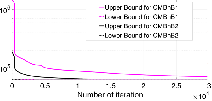
Figure 3: Upper and lower bound evolution in branch-and-bound.

4.2 Qualitative comparisons

To highlight the importance of globally optimal CM, we tested on select $10$ ms subsequences (about $N=50k$ events each) from the boxes data [15]—in the next experiment, a more comprehensive experiment and quantitative benchmarking will be described. Here, on the subsequences chosen, we compared BnB against the following methods:

• CMGD1: locally optimal solver (fmincon from Matlab) was used to perform CM with initialisation $\bm{\omega}=0$ (equivalent to identity rotation).

• CMGD2: same as above, but initialised with the optimised $\bm{\omega}$ from the previous $10$ ms time window.

Both local methods were executed on the continuous event image with Gaussian kernel of bandwidth $1$ pixel.

Fig. 4 depicts motion compensated event images from two subsequences (Subseq 1 and Subseq 2); see supplementary material for more results. The examined cases show that the local methods (both CMGD1 and CMGD2) can indeed often converge to bad local solutions. Contrast this to BnB which always produced sharp event images.

These results also show that CM based on continuous and discrete event images yield practically identical solutions. Since CMBnB2 usually converges much faster than CMBnB1, we use CMBnB2 in the remaining experiments.

	CMBnB1	CMBnB2	CMGD1	CMGD2
Subseq 1
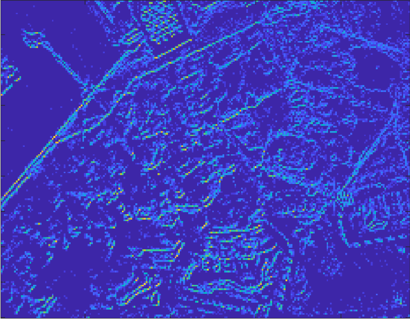
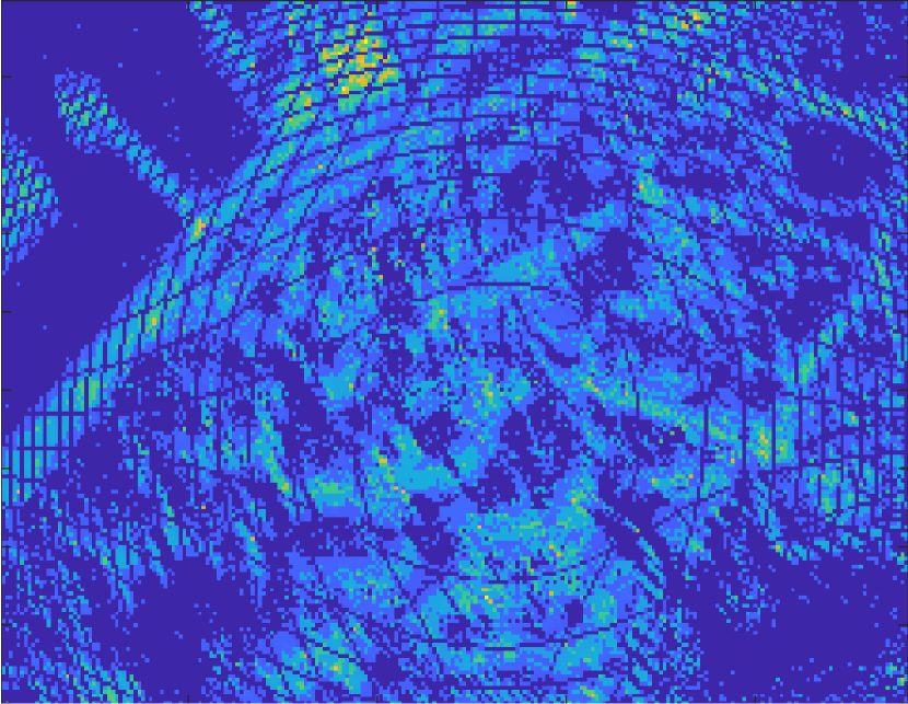
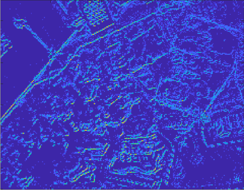
Subseq 2

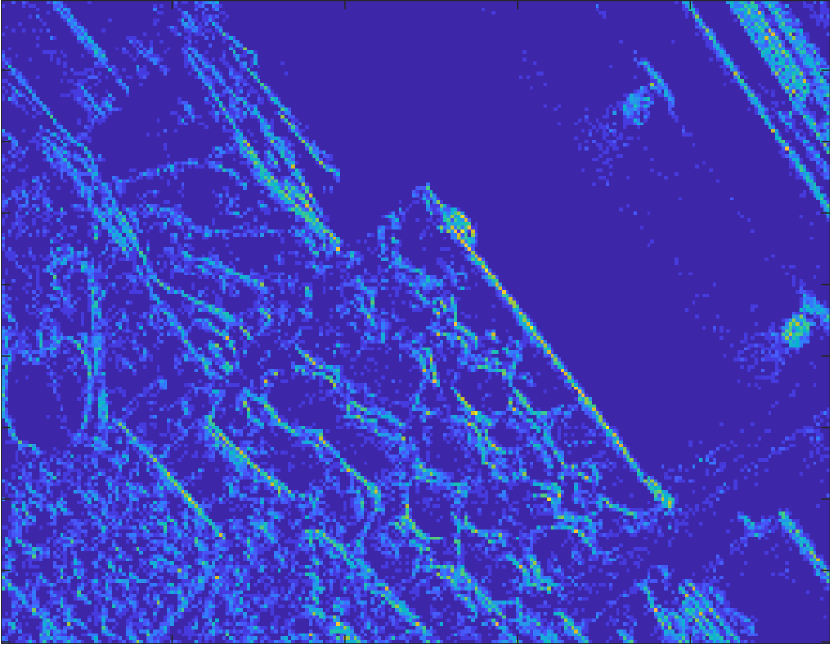
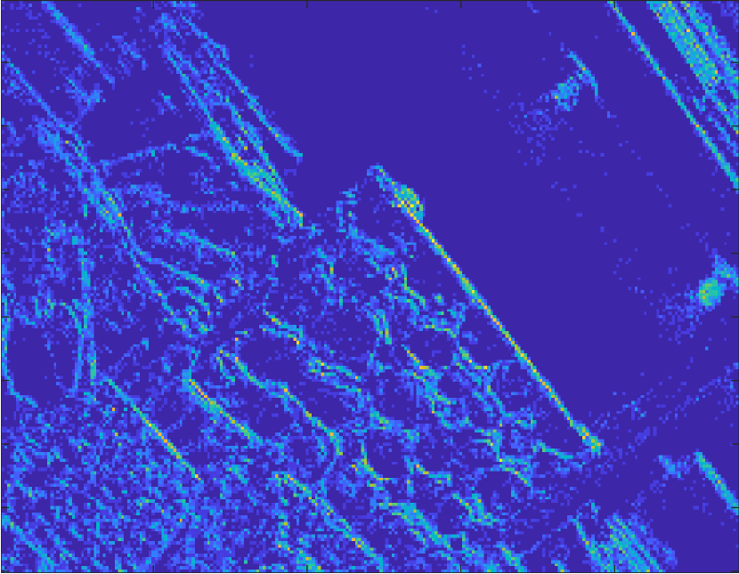
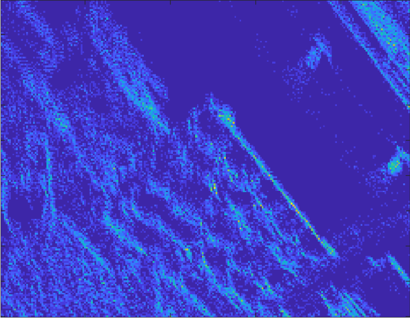
Figure 4: Qualitative results (motion compensated event images) from Subseq 1 and Subseq 2 of boxes.

4.3 Quantitative benchmarking

We performed benchmarking using publicly available datasets [24, 8]. We introduced two additional variants to CMGD1 and CMGD2:

• CMRW1: A variant of CM [31] that uses a different objective function (called reward):

  $$Rw(\bm{\omega})=C(\bm{\omega})+\dfrac{1}{P}\sum_{j=1}^{P}(e^{(-H(\mathbf{x}_{j};\bm{\omega}))}+e^{(H(\mathbf{x}_{j};\bm{\omega}))}).$$

  The initial solution is taken as $\bm{\omega}=0$.

• CMRW2: Same as CMRW1 but initialised with the optimised $\bm{\omega}$ from the previous subsequence.

We also compared against EventNet [29], which is based on deep learning. However, similar to the error reported in [29], we found that the error for EventNet was much higher than the error of the CM methods (e.g., the translated angular velocity error of the maximum of EventNet is 17.1%, while it is around 5% for CM). The lack of publicly available implementation also hampered objective testing of EventNet. We thus leave comparisons against deep learning methods as future work.

4.3.1 Rotational motion in indoor scene

We used event sequences poster, boxes and dynamic from [15, 24], which were recorded using a Davis 240C [4] under rotational motion over a static indoor scene. The ground truth motion was captured using a motion capture system. Each sequence has a duration of $1$ minute and around $100$ million events. For these sequences, the rotational motion was minor in a large part of the sequences (thereby producing trivial instances to CM), thus in our experiment we used only the final $15$ seconds of each sequence, which tended to have more significant motions.

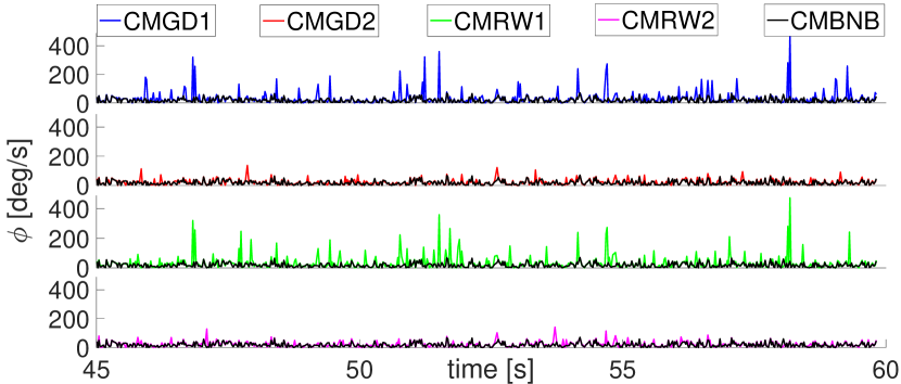
(a) boxes

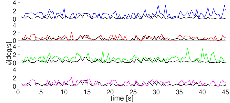
(b) Sequence 1

Figure 5: Error $\phi$ of all CM methods (plotted against time) for (a) boxes sequence [15] and (b) Sequence 1 of [8]. In each subplot, the error of CMBNB is superimposed for reference.

We split each sequence into contiguous $10$ ms subsequences which were then subject to CM. For boxes and poster, each CM instance was of size $N\approx 50k$, while for dynamic, each instance was of size $N\approx 25k$. For each CM instance, let $\bar{\bm{\omega}}$ and $\hat{\bm{\omega}}$ be the ground truth and estimated parameters. An error metric we used is

$$\epsilon=\|\bar{\bm{\omega}}-\hat{\bm{\omega}}\|_{2}.$$ (42)

Our second error metric, which considers only differences in angular rate, is

$$\phi=\lvert\|\bar{\bm{\omega}}\|_{2}-\|\hat{\bm{\omega}}\|_{2}\rvert.$$ (43)

Fig. 5a plots $\epsilon$ over all the CM instances for the boxes sequence, while Table 1 shows the average ($\mu$) and standard deviation ($\sigma$) of $\epsilon$ and $\phi$ over all CM instances.

Amongst the local methods, the different objective functions did not yield significant differences in quality. The more important observation was that CMGD2/CMRW2 gave solutions of much higher quality than CMGD1/CMRW1, which confirms that good initialisation is essential for the local methods. Due to its exact nature, CMBnB provided the best quality in rotation estimation; its standard deviation of $\epsilon$ is also lower, indicating a higher stability over the sequences. Moreover, CMBnB does not require any initialisation, unlike the local methods.

For the three sequences used (dynamic, boxes, poster), the maximum absolute angular velocities are $500$, $670$ and $1000$ deg/s respectively [15, 24]. The average $\phi$ error of CMBnB of $10.09$, $17.97$ and $46.34$ deg/s thus translate into $2.2\%$, $2.7\%$ and $4.6\%$ of the maximum, respectively.

Runtime

The average runtimes of CMBnB over all instances in the three sequences (dynamic, boxes, poster) were $163.2$, $278.3$ and $320.6$ seconds. CMGD optimised with the conjugate gradient solver in fmincon has average runtimes of $20.2$, $31.1$ and $35.3$ seconds.

Method	dynamic				boxes				poster
	$\mu(\epsilon)$	$\mu(\phi)$	$\sigma(\epsilon)$	$\sigma(\phi)$	$\mu(\epsilon)$	$\mu(\phi)$	$\sigma(\epsilon)$	$\sigma(\phi)$	$\mu(\epsilon)$	$\mu(\phi)$	$\sigma(\epsilon)$	$\sigma(\phi)$
CMGD1	21.52	20.07	24.38	31.13	31.29	31.47	34.30	45.94	56.58	54.92	47.03	58.95
CMGD2	15.09	13.31	10.39	12.08	22.01	21.70	12.79	18.83	49.64	50.12	35.93	42.77
CMRW1	21.03	18.59	25.41	28.83	32.28	32.23	36.11	46.01	59.03	58.71	49.49	60.87
CMRW2	14.55	12.29	9.85	11.21	21.95	21.41	13.71	18.42	49.49	50.04	37.51	43.35
CMBnB	11.93	10.09	7.82	8.74	18.76	17.97	10.06	14.66	44.34	46.34	24.79	36.79

Table 1: Average and standard deviation of $\epsilon$ and $\phi$ over all CM instances in boxes, dynamic, and poster (best result bolded).

4.3.2 Attitude estimation

We repeated the above experiment on the event-based star tracking (attitude estimation) dataset of [8, 7], which contains $11$ event sequences of rotational motion over a star field. Each sequence has a constant angular velocity of $4$ deg/s over a duration of $45$ seconds and around $1.5$ million events. We split each sequence into $400$ ms subsequences, which yielded $N\approx 15,000$ events per subsequence. Fig. 5b plots the $\phi$ errors for Sequence 1 in the dataset. The average errors and standard deviation over all CM instances are shown in Table 2. Again, CMBnB gave the highest quality solutions; its average $\phi$ error of $0.234$ deg/s translate into $5.8\%$ of the maximum. The average runtime of CMBnB and CMGD over all instances were $80.7$ and $11.1$ seconds.

Method	$\mu(\epsilon)$	$\mu(\phi)$	$\sigma(\epsilon)$	$\sigma(\phi)$
CMGD1	0.448	0.652	0.314	0.486
CMGD2	0.294	0.423	0.232	0.323
CMRW1	0.429	0.601	0.346	0.468
CMRW2	0.318	0.461	0.234	0.341
CMBnB	0.174	0.234	0.168	0.217

Table 2: Average and standard deviation of $\epsilon$ and $\phi$ over all CM instances in the star tracking dataset (best result bolded).

5 Conclusions

We proposed a novel globally optimal algorithm for CM based on BnB. The theoretical validity of our algorithm has been established, and the experiments showed that it greatly outperformed local methods in terms of solution quality.

A Geometric derivations of the elliptical region

Here we present the analytic form of the centre $\mathbf{c}$, semi-major axis $\mathbf{y}$, and semi-minor axis $\mathbf{z}$ of the elliptical region $\mathcal{L}$ (see Sec. 3) following the method in [22, 9] (subscript $i$ and explicit dependency on $\mathbb{B}$ are omitted for simplicity). See Fig. 2a in the main text for a visual representation of the aforementioned geometric entities.

1. Calculate direction of the cone-beam

   $$\hat{\mathbf{u}}=\dfrac{\mathbf{R}(t;\bm{\omega}_{\mathbf{c}})\tilde{\mathbf{u}}}{\|\mathbf{R}(t;\bm{\omega}_{\mathbf{c}})\tilde{\mathbf{u}}\|_{2}},$$ (44)

   its radius

   $$r=\sin{\alpha({\mathbb{B}})},$$ (45)

   and the norm vector to the image plane $\hat{\mathbf{n}}=[0\;0\;1]^{T}$.

2. Calculate the semi-major axis direction within the cone-beam

   $$\hat{\mathbf{y}}=\dfrac{\hat{\mathbf{u}}\times(\hat{\mathbf{u}}\times\hat{\mathbf{n}})}{\|\hat{\mathbf{u}}\times(\hat{\mathbf{u}}\times\hat{\mathbf{n}})\|}$$ (46)

   and semi-minor axis direction

   $$\hat{\mathbf{z}}=\dfrac{\hat{\mathbf{y}}\times\hat{\mathbf{n}}}{\|\hat{\mathbf{y}}\times\hat{\mathbf{n}}\|}.$$ (47)

3. Calculate the intersecting points between the ray with the direction of the semi-major axis and the cone-beam

   $$\mathbf{y}^{(a)} =\hat{\mathbf{u}}-r\hat{\mathbf{y}}$$ (48)

   $$\mathbf{y}^{(b)} =\hat{\mathbf{u}}+r\hat{\mathbf{y}},$$

   and the analogous points for the semi-minor axis

   $$\mathbf{z}^{(a)} =\hat{\mathbf{u}}-r\hat{\mathbf{z}}$$ (49)

   $$\mathbf{z}^{(b)} =\hat{\mathbf{u}}+r\hat{\mathbf{z}}.$$

4. Obtain $\mathbf{y}^{\prime(a)}$, $\mathbf{y}^{\prime(b)}$, $\mathbf{z}^{\prime(a)}$ and $\mathbf{z}^{\prime(b)}$ as the projection of (48) and (49) into the image plane with the intrinsic matrix $\mathbf{K}$.

5. Calculate $\mathbf{c}=0.5(\mathbf{y}^{\prime(a)}+\mathbf{y}^{\prime(b)})$, $\mathbf{y}=\|\mathbf{y}^{\prime(a)}-\mathbf{y}^{\prime(b)}\|_{2}$, and $\mathbf{z}=\|\mathbf{z}^{\prime(a)}-\mathbf{z}^{\prime(b)}\|_{2}$.

B Proofs

We state our integer quadratic problem again.

$$\begin{aligned} \overline{S}^{*}_{d}(\mathbb{B})=\max_{\mathbf{Z}\in\{0,1\}^{N\times K}}\quad&\sum^{K}_{k=1}\left(\sum_{i=1}^{N}\mathbf{Z}_{i,k}\mathbf{M}_{i,k}\right)^{2}\\ \text{s.t.}\quad&\mathbf{Z}_{i,k}\leq\mathbf{M}_{i,k},\;\;\forall i,k,\\ &\sum_{k=1}^{K}\mathbf{Z}_{i,k}=1,\;\;\forall i.\end{aligned}$$ (IQP)

B.1 Proof of Lemma 1 in the main text

Lemma 5.

$$\overline{H}_{c}(\mathbf{x}_{j};\mathbb{B})\geq\max_{\bm{\omega}\in\mathbb{B}}\leavevmode\nobreak\ H_{c}(\mathbf{x}_{j};\bm{\omega})$$ (50)

with equality achieved if $\mathbb{B}$ is singleton, i.e., $\mathbb{B}=\{\bm{\omega}\}$.

Proof.

This lemma can be demonstrated by contradiction. Let $\bm{\omega}^{*}$ be the optimiser for the RHS of (50). If

$$H_{c}(\mathbf{x}_{j};\bm{\omega}^{*})>\overline{H}_{c}(\mathbf{x}_{j};\mathbb{B}),$$ (51)

it follows from the definition of pixel intensity (Eq. (1) ) and its upper bound (Eq. (23)) that

$$\|\mathbf{x}_{j}-f(\mathbf{u}_{i},t_{i},\bm{\omega}^{*})\|<\max\left(\|\mathbf{x}_{j}-\mathbf{c}_{i}(\mathbb{B})\|-\|\mathbf{y}_{i}(\mathbb{B})\|,0\right),$$ (52)

for at least one $i=1,\ldots,N$.

In words, the shortest distance between $\mathbf{x}_{j}$ and the disc $\mathcal{D}_{i}(\mathbb{B})$ is greater than the distance between $\mathbf{x}_{j}$ and the optimal position $f(\mathbf{u}_{i},t_{i},\bm{\omega}^{*})$. However, $f(\mathbf{u}_{i},t_{i},\bm{\omega}^{*})$ is always inside the disc $\mathcal{D}_{i}(\mathbb{B})$, and hence Eq. (52) cannot hold. If $\mathbb{B}=\{\bm{\omega}\}$, then from definition (23) in the main text $\overline{H}_{c}(\mathbf{x}_{j};\mathbb{B})=H_{c}(\mathbf{x}_{j};\bm{\omega})$. ∎

B.2 Proof of Lemma 2 in the main text

Lemma 6.

$$\overline{S}^{*}_{d}(\mathbb{B})\geq\max_{\bm{\omega}\in\mathbb{B}}\leavevmode\nobreak\ \sum_{j=1}^{P}H_{d}(\mathbf{x}_{j};\bm{\omega})^{2},$$ (53)

with equality achieved if $\mathbb{B}$ is singleton, i.e., $\mathbb{B}=\{\bm{\omega}\}$.

Proof.

We pixel-wisely reformulate IQP:

$$\begin{aligned} \overline{S}^{*}_{d}(\mathbb{B})=\max_{\mathbf{Q}\in\{0,1\}^{N\times P}}\quad&\sum^{P}_{j=1}\left(\sum_{i=1}^{N}\mathbf{Q}_{i,j}\right)^{2}\\ \text{s.t.}\quad&\mathbf{Q}_{i,j}\leq\mathbf{T}_{i,j},\;\;\forall i,j,\\ &\sum_{j=1}^{P}\mathbf{Q}_{i,j}=1,\;\;\forall i,\end{aligned}$$ (P-IQP)

and we express the RHS of (53) as a mixed integer quadratic program:

$$\begin{aligned} \max_{\bm{\omega}\in\mathbb{B},\mathbf{Q}\in\{0,1\}^{N\times P}}\quad&\sum^{P}_{j=1}\left(\sum_{i=1}^{N}\mathbf{Q}_{i,j}\right)^{2}\\ \text{s.t.}\quad&\mathbf{Q}_{i,j}=\mathbb{I}(f(\mathbf{u}_{i},t_{i};\,\bm{\omega})\leavevmode\nobreak\ \text{in}\leavevmode\nobreak\ \mathbf{x}_{j}),\;\forall i,j.\end{aligned}$$ (MIQP)

Problem P-IQP is a relaxed version of MIQP - hence (53) holds - as for every $\bm{e}_{i}$, the feasible pixel $\mathbf{x}_{j}$ is in $\mathcal{D}_{i}(\mathbb{B})$; whereas for MIQP, the feasible pixel is dictated by a single $\bm{\omega}\in\mathbb{B}$. If $\mathbb{B}$ collapses into $\bm{\omega}$, every event $\bm{e}_{i}$ can intersect only one pixel $\mathbf{x}_{j}$, hence $\mathbf{T}_{i,j}=\mathbb{I}(f(\mathbf{u}_{i},t_{i};\,\bm{\omega})\leavevmode\nobreak\ \text{in}\leavevmode\nobreak\ \mathbf{x}_{j}),\;\forall i,j$; $\sum_{j=1}^{P}\mathbf{T}_{i,j}=1,\;\forall i$; and $\sum_{j=1}^{P}\mathbf{Q}_{i,j}=1\implies\mathbf{Q}_{i,j}=\mathbf{T}_{i.j},\forall i$; therefore, MIQP is equivalent to P-IQP if $\mathbb{B}=\{\bm{\omega}\}$.

∎

B.3 Proof of Lemma 3 in the main text

Lemma 7.

Problem IQP has the same solution if $\mathbf{M}$ is replaced with $\mathbf{M}^{\prime}$.

Proof.

We show that removing an arbitrary non-dominant column from $\mathbf{M}$ does not change the solution of IQP. Without loss of generality, assume the last column of $\mathbf{M}$ is non-dominant. Equivalent to solving IQP on $\mathbf{M}$ without its last column is the following IQP reformulation:

$$\overline{S}^{*}_{d}(\mathbb{B})=\max_{\mathbf{Z}\in\{0,1\}^{N\times K}}\quad \sum^{K-1}_{k=1}\left(\sum_{i=1}^{N}\mathbf{Z}_{i,k}\mathbf{M}_{i,k}\right)^{2}+$$ (54a)

$$\left(\sum_{i=1}^{N}\mathbf{Z}_{i,K}\mathbf{M}_{i,K}\right)^{2}$$ (54b)

s.t. $$\mathbf{Z}_{i,k}\leq\mathbf{M}_{i,k},\;\;\forall i,k,$$ (54c)

$$\sum_{k=1}^{K}\mathbf{Z}_{i,k}=1,\;\;\forall i,$$ (54d)

$$\mathbf{Z}_{i,K}=0,\;\;\forall i,$$ (54e)

which is same as IQP but with additional constraint (54e). Since $\mathbf{M}_{:,K}$ is non-dominant, it must exists a dominant column $\mathbf{M}_{:,\eta}$ such that

$$\mathbf{M}_{i,K}\leq\mathbf{M}_{i,\eta},\;\;\forall i.$$ (55)

Hence, if $\mathbf{M}_{i,K}=1$, then $\mathbf{M}_{i,\eta}=1$ must holds $\forall i$. Let $\mathbf{Z}^{*}$ be the optimiser of IQP with $\mathbf{Z}^{*}_{i_{a},K},\ldots,\mathbf{Z}^{*}_{i_{b},K}=1$. Let define $\mathbf{Z}^{\prime*}$ same as $\mathbf{Z}^{*}$ but with $\mathbf{Z}^{\prime*}_{:,K}=\mathbf{0}$ and $\mathbf{Z}^{\prime*}_{i_{a},\eta},\ldots,\mathbf{Z}^{\prime*}_{i_{b},\eta}=1$. In words, we “move” the $1$ values from the last column to its dominant one. We show that $\mathbf{Z}^{\prime*}$ is an equivalent solution (same objective value than $\mathbf{Z}^{*}$). $\mathbf{Z}^{\prime*}$ is feasible since (55) ensures condition (54c), (54d) is not affected by “moving ones” in the same row, and (54e) is true for the definition of $\mathbf{Z}^{\prime*}$. Finally we show that

$$\sum_{i=1}^{N}\mathbf{Z}^{*}_{i,K}\mathbf{M}_{i,K}=\sum_{i=1}^{N}\mathbf{Z}^{\prime*}_{i,\eta}\mathbf{M}_{i,\eta}$$ (56)

therefore $\mathbf{Z}^{\prime*}$ produces same objective value than IQP. We prove (56) by contradiction. Assume exists at least one $i^{\prime}\not\in\{i_{a},\ldots,i_{b}\}$ such that $\mathbf{Z}^{*}_{i^{\prime},\eta}=1\implies\mathbf{Z}^{\prime*}_{i^{\prime},\eta}=1$. Then, $\mathbf{Z}^{\prime*}$ produces a larger objective value than $\mathbf{Z}^{*}$ which is a contradiction since problem (54) is most restricted than IQP. Thus, removing any arbitrary non-dominant column will not change the solution which implies this is also true if we remove all non-dominant columns (i.e., if we replace $\mathbf{M}$ with $\mathbf{M}^{\prime}$).

∎

B.4 Proof of Lemma 4 in the main text

Lemma 8.

$$\overline{S}_{d}(\mathbb{B})\geq\overline{S}^{*}_{d}(\mathbb{B})$$ (57)

with equality achieved if $\mathbb{B}$ is singleton, i.e., $\mathbb{B}=\{\bm{\omega}\}$.

Proof.

To prove (57), it is enough to show

$$\begin{aligned} \overline{S}_{d}(\mathbb{B})=\max_{\mathbf{Z}\in\{0,1\}^{N\times K^{\prime}}}\quad&\sum^{K^{\prime}}_{k=1}\left(\sum_{i=1}^{N}\mathbf{Z}_{i,k}\mathbf{M}^{\prime}_{i,k}\right)^{2}\\ \text{s.t.}\quad&\mathbf{Z}_{i,k}\leq\mathbf{M}^{\prime}_{i,k},\;\;\forall i,k,\\ &\sum_{k=1}^{K^{\prime}}\sum^{N}_{i=1}\mathbf{Z}_{i,k}=N,\end{aligned}$$ (R-IQP)

is a valid relaxation of IQP. This is true as the constraint $\sum_{k=1}^{K^{\prime}}\sum^{N}_{i=1}\mathbf{Z}_{i,k}=N$ in R-IQP is a necessary but not sufficient condition for the constraints $\sum_{k=1}^{K^{\prime}}\mathbf{Z}_{i,k}=1,\forall i$ in IQP. If $\mathbb{B}$ collapse into $\bm{\omega}$, every event $\bm{e}_{i}$ can intersect only one CC $\mathcal{G}_{k}\implies\sum_{k=1}^{K^{\prime}}\mathbf{Z}_{i,k}=1$; hence, R-IQP is equivalent to IQP. ∎

B.5 Proof of lower bound (39) in the main text

Lemma 9.

$$\underline{H}_{c}(\mathbf{x}_{j};\mathbb{B})\leq\min_{\bm{\omega}\in\mathbb{B}}\leavevmode\nobreak\ H_{c}(\mathbf{x}_{j};\bm{\omega})$$ (58)

with equality achieved if $\mathbb{B}$ is singleton, i.e., $\mathbb{B}=\{\bm{\omega}\}$.

Proof.

Analogous to Lemma 5, we prove this Lemma by contraction. Let $\bm{\omega}^{*}$ be the optimiser for the RHS of (58). If

$$H_{c}(\mathbf{x}_{j};\bm{\omega}^{*})<\underline{H}_{c}(\mathbf{x}_{j};\mathbb{B}),$$ (59)

it follows from the definition of pixel intensity (Eq. (1)) and its lower bound (Eq. (39)) that

$$\|\mathbf{x}_{j}-f(\mathbf{u}_{i},t_{i},\bm{\omega}^{*})\|>\|\mathbf{x}_{j}-\mathbf{c}_{i}(\mathbb{B})\|+\|\mathbf{y}_{i}(\mathbb{B})\|,$$ (60)

for at least one $i=1,\ldots,N$.

In words, the longest distance between $\mathbf{x}_{j}$ and the disc $\mathcal{D}_{i}(\mathbb{B})$ is less than the distance between $\mathbf{x}_{j}$ and the optimal position $f(\mathbf{u}_{i},t_{i},\bm{\omega}^{*})$. However, $f(\mathbf{u}_{i},t_{i},\bm{\omega}^{*})$ is always inside the disc $\mathcal{D}_{i}(\mathbb{B})$, and hence Eq. (60) cannot hold. If $\mathbb{B}=\{\bm{\omega}\}$, then from definition (39) in the main text $\underline{H}_{c}(\mathbf{x}_{j};\mathbb{B})=H_{c}(\mathbf{x}_{j};\bm{\omega})$.

∎

B.6 Proof of lower bound (41) in the main text

Lemma 10.

$$\underline{\mu}_{d}(\mathbb{B})\leq\min_{\bm{\omega}\in\mathbb{B}}\leavevmode\nobreak\ \dfrac{1}{P}\sum_{j=1}^{P}H_{d}(\mathbf{x}_{j};\bm{\omega}),$$ (61)

with equality achieved if $\mathbb{B}$ is singleton, i.e., $\mathbb{B}=\{\bm{\omega}\}$.

Proof.

This lemma can be demonstrated by contraction. Let $\bm{\omega}^{*}$ be the optimiser of the RHS of (61). If

$$\dfrac{1}{P}\sum_{j=1}^{P}H_{d}(\mathbf{x}_{j};\bm{\omega}^{*})<\underline{\mu}_{d}(\mathbb{B}),$$ (62)

after replacing the pixel intensity and the lower bound pixel value with they definitions (Eqs. (3) and (41)) in (62), it leads to

$$\sum_{i=1}^{N}\sum_{j=1}^{P}\mathbb{I}(f(\mathbf{u}_{i},t_{i};\,\bm{\omega}^{*})\leavevmode\nobreak\ \text{lies in pixel}\leavevmode\nobreak\ \mathbf{x}_{j})$$ (63a)

$$< \sum_{i=1}^{N}\mathbb{I}(\mathcal{D}_{i}\leavevmode\nobreak\ \text{fully lie in the image plane}).$$ (63b)

In words, for every warped event $f(\mathbf{u}_{i},t_{i};\,\bm{\omega}^{*})\in\mathcal{D}_{i}$ that lies in any pixel $\mathbf{x}_{j}\in X$ of the image plane, the discs $\mathcal{D}_{i}$ must fully lie in the image plane. Since (63a) is a less restricted problem than (63b), (62) cannot hold. If $\mathbb{B}=\{\bm{\omega}\}$, $\mathcal{D}_{i}=f(\mathbf{u}_{i},t_{i};\,\bm{\omega})$; therefore, the two sides in (61) are equivalent.

∎

C Additional qualitative results

Figs. 6, 7 and 8 show additional motion compensation results (Sec. 4.2 in the main text) for subsequences from boxes, dynamic and poster.

	CMBnB1	CMBnB2	CMGD1	CMGD2
Subseq 3
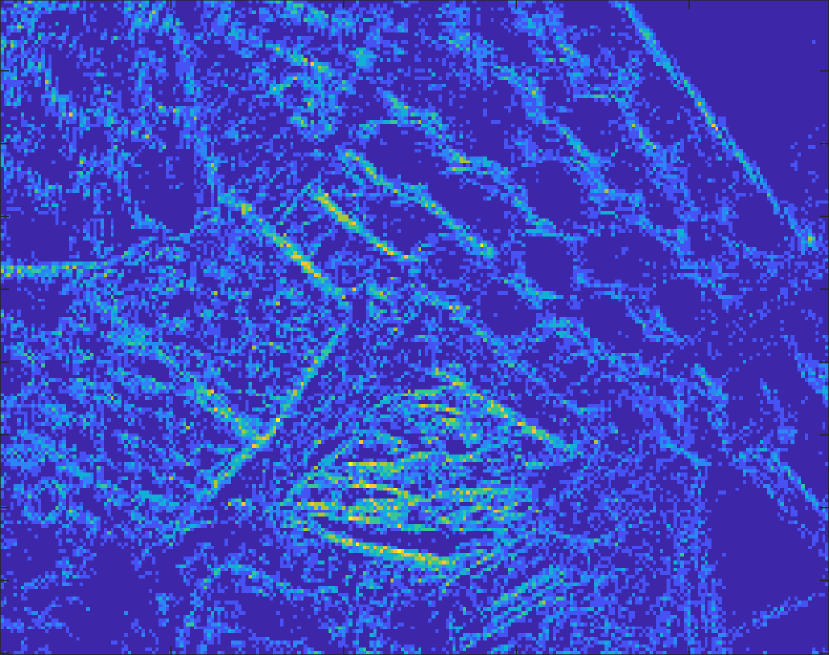
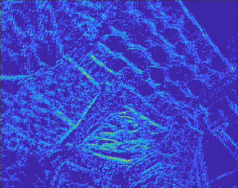
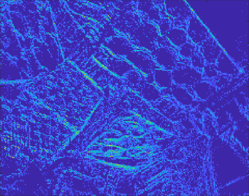
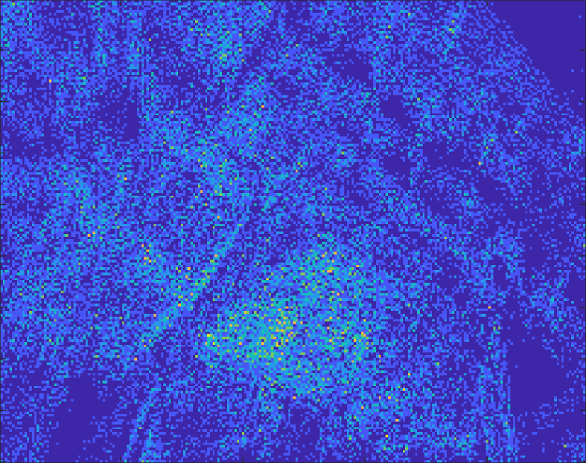
Subseq 4
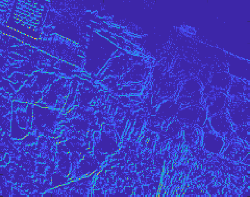
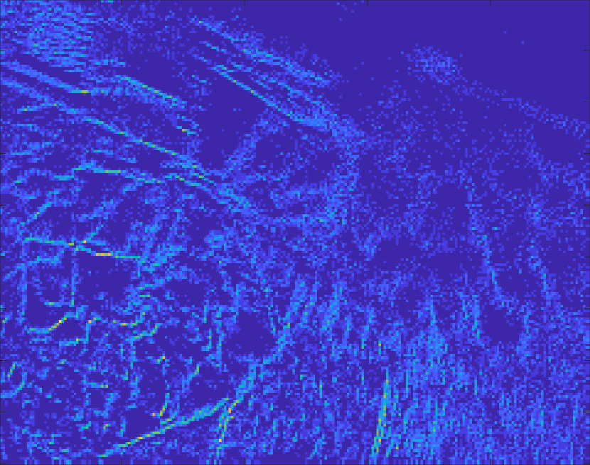
Subseq 5

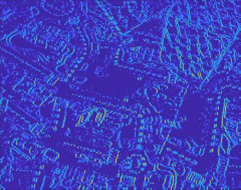
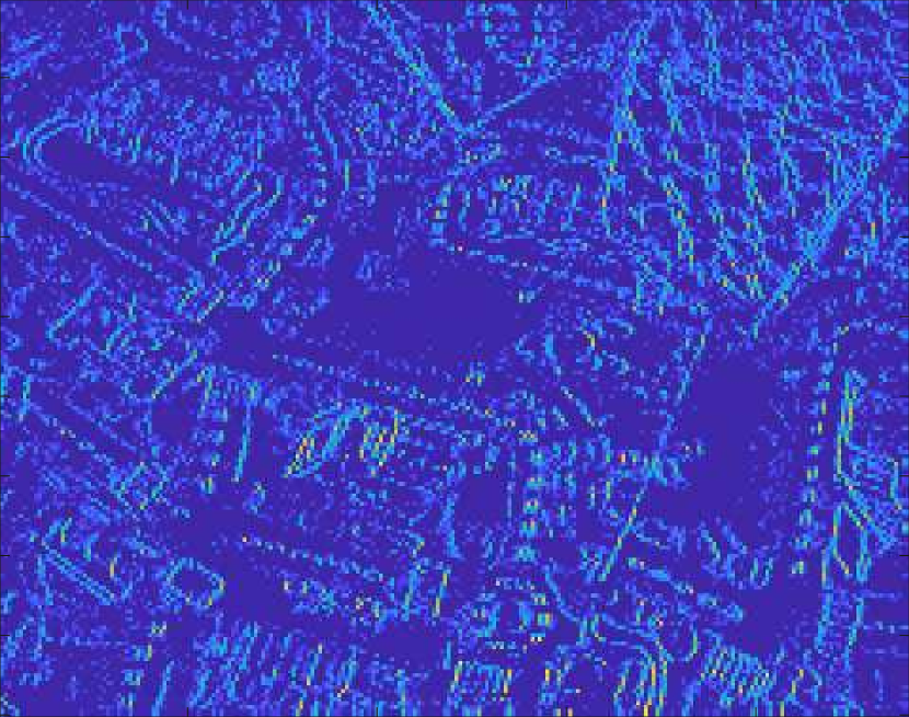
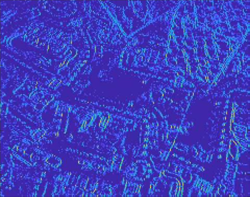
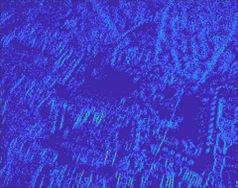
Figure 6: Qualitative results (motion compensated event images) for boxes.

	CMBnB1	CMBnB2	CMGD1	CMGD2
Subseq 1
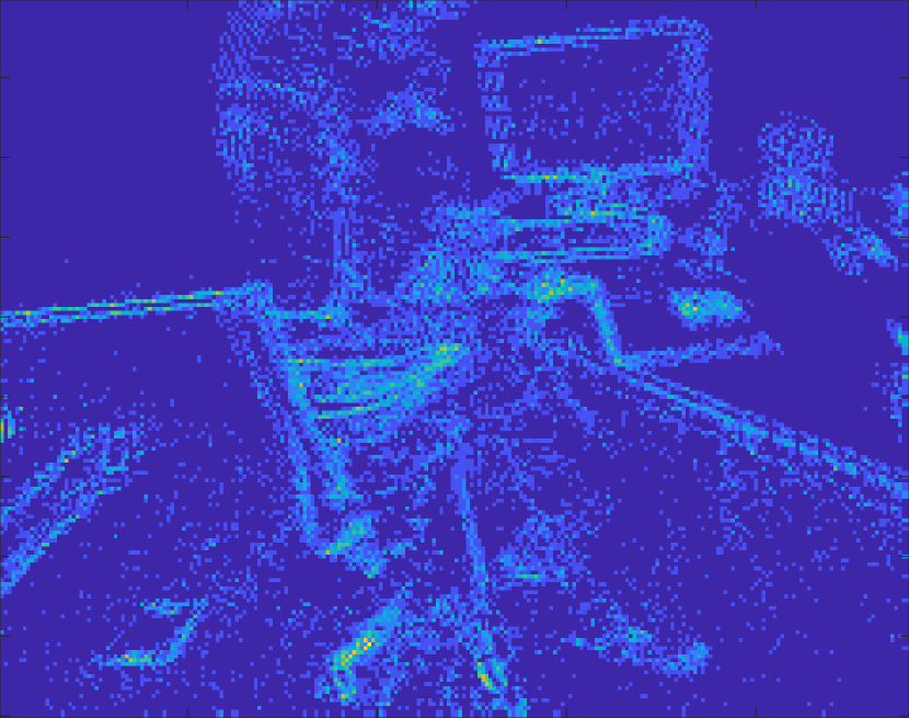
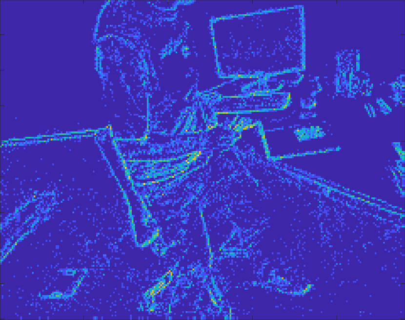
Subseq 2
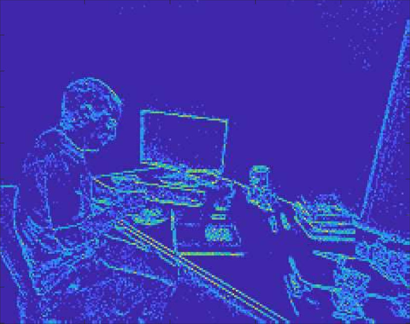
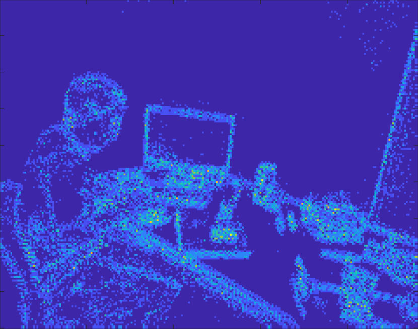
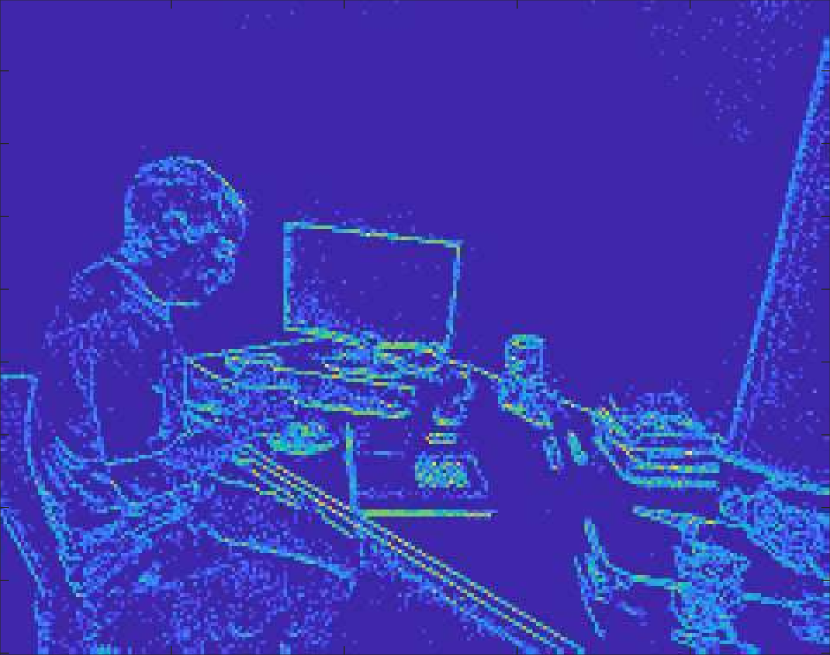
Subseq 3
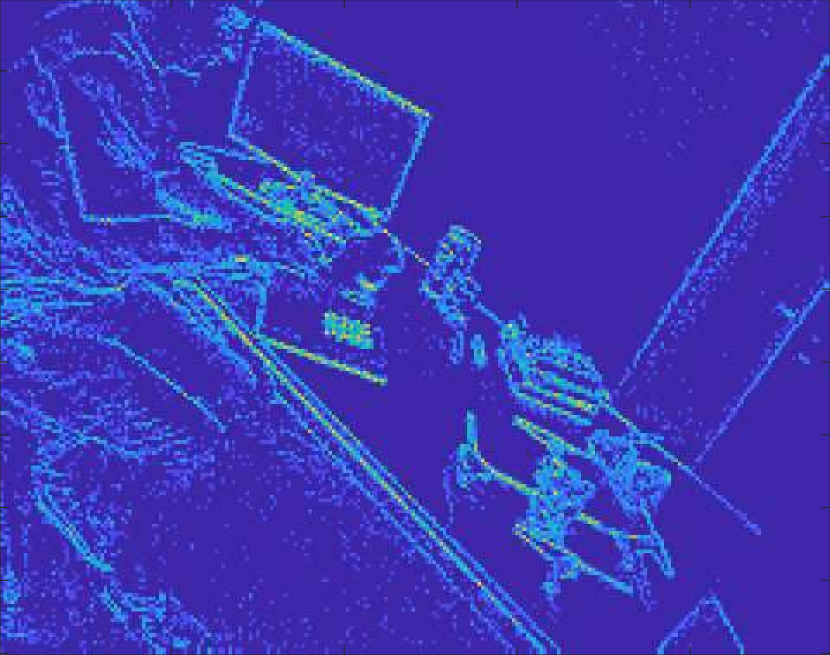
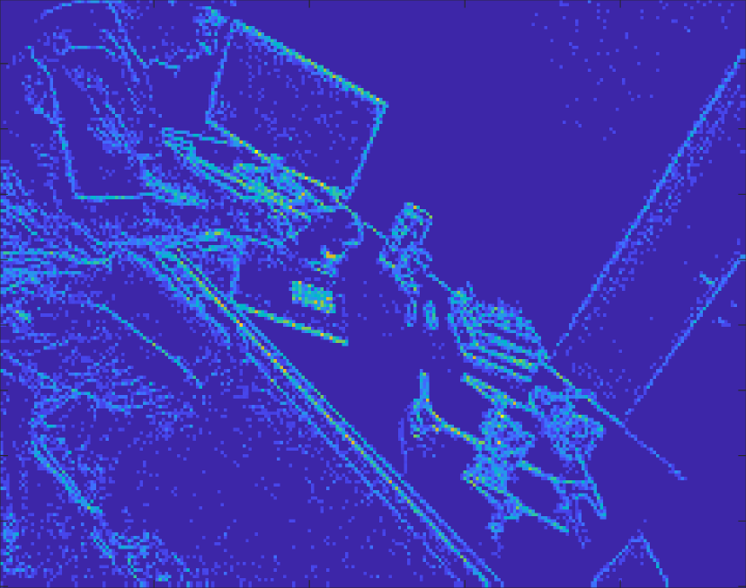
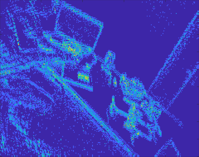
Subseq 4
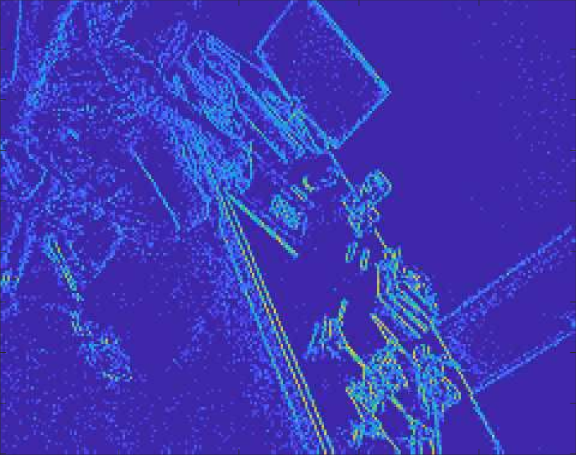
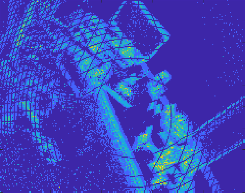
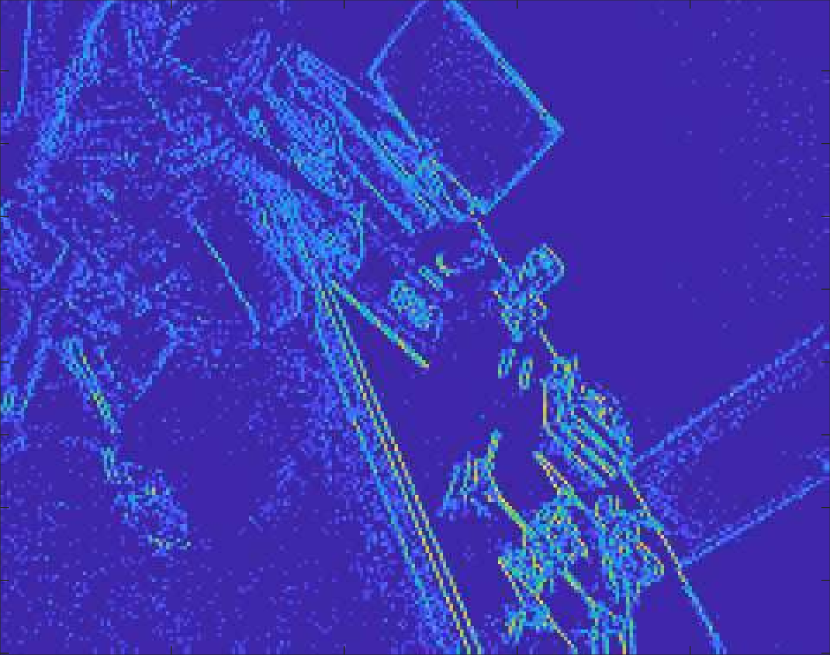
Subseq 5

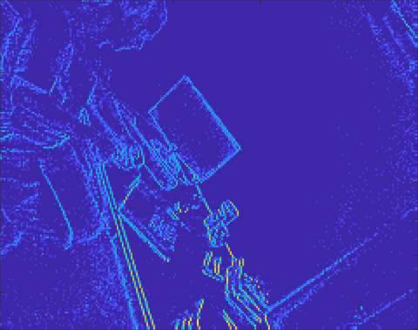
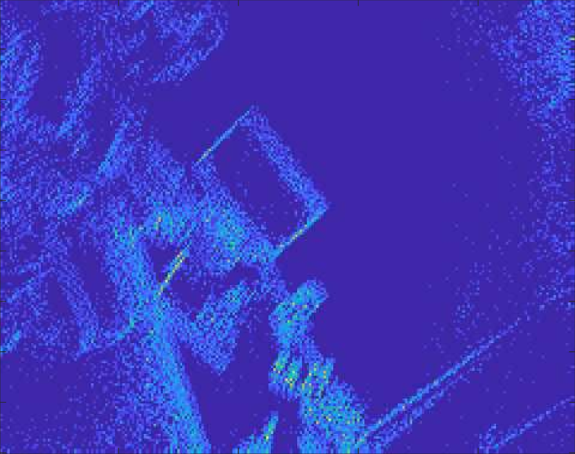
Figure 7: Qualitative results (motion compensated event images) for dynamic.

	CMBnB1	CMBnB2	CMGD1	CMGD2
Subseq 1
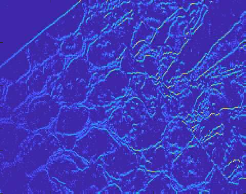
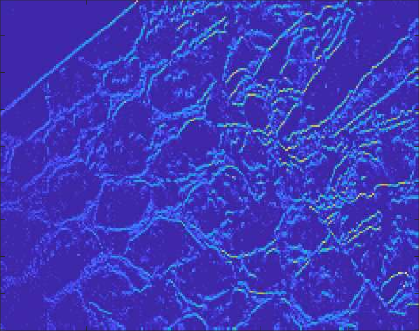
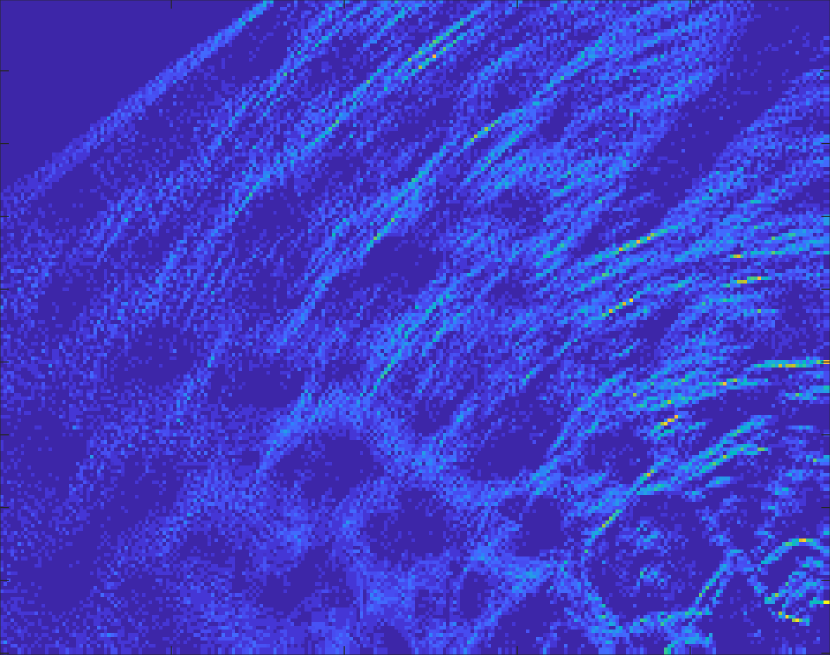
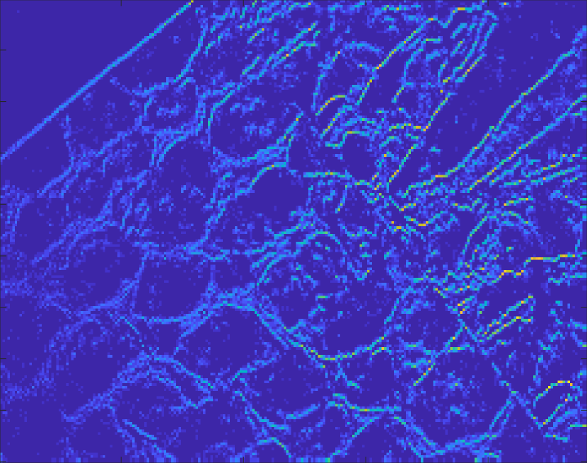
Subseq 2
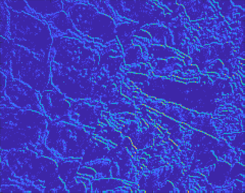
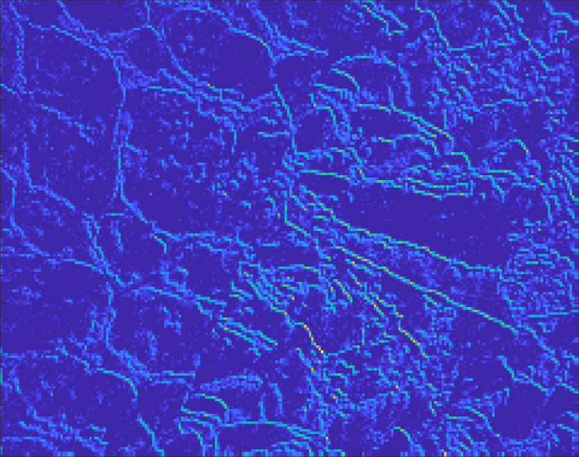
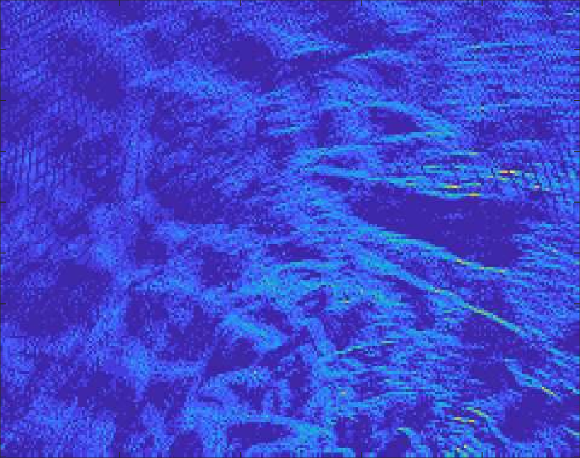
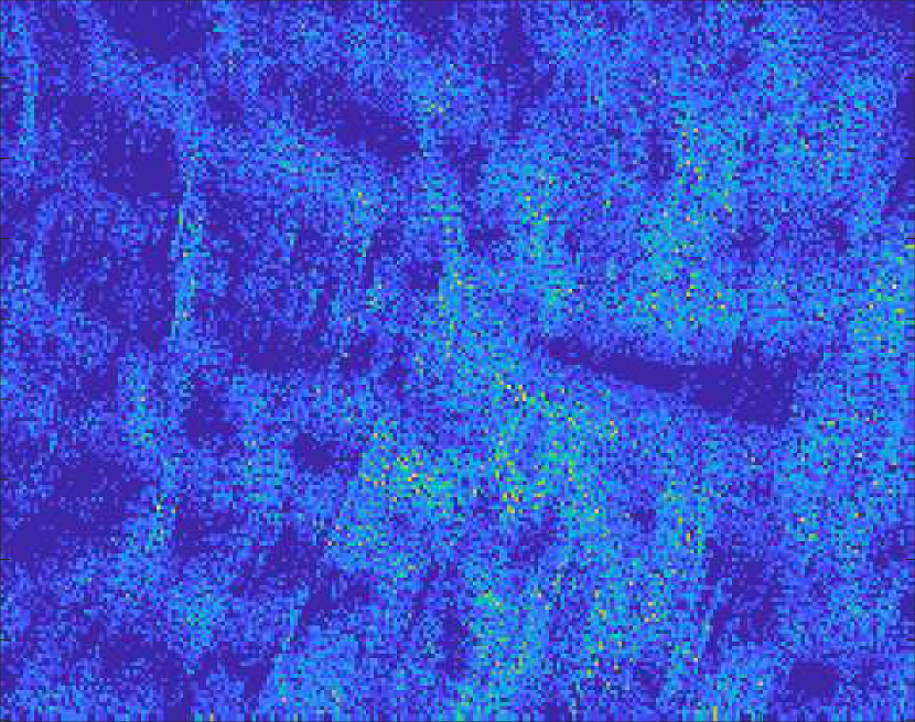
Subseq 3
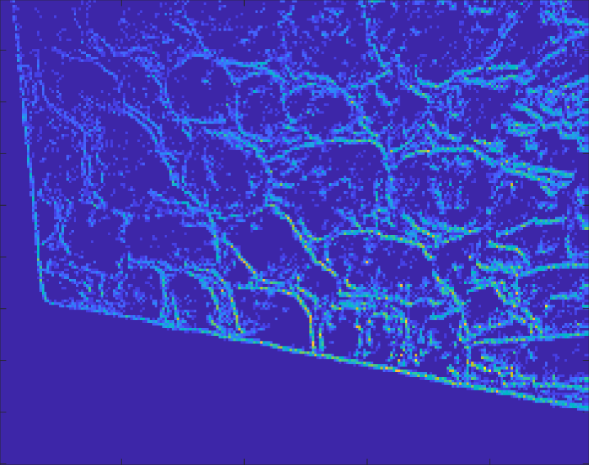
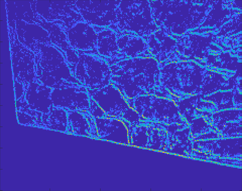
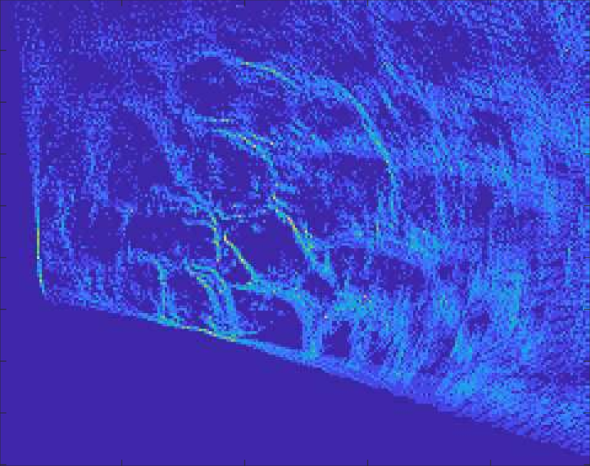
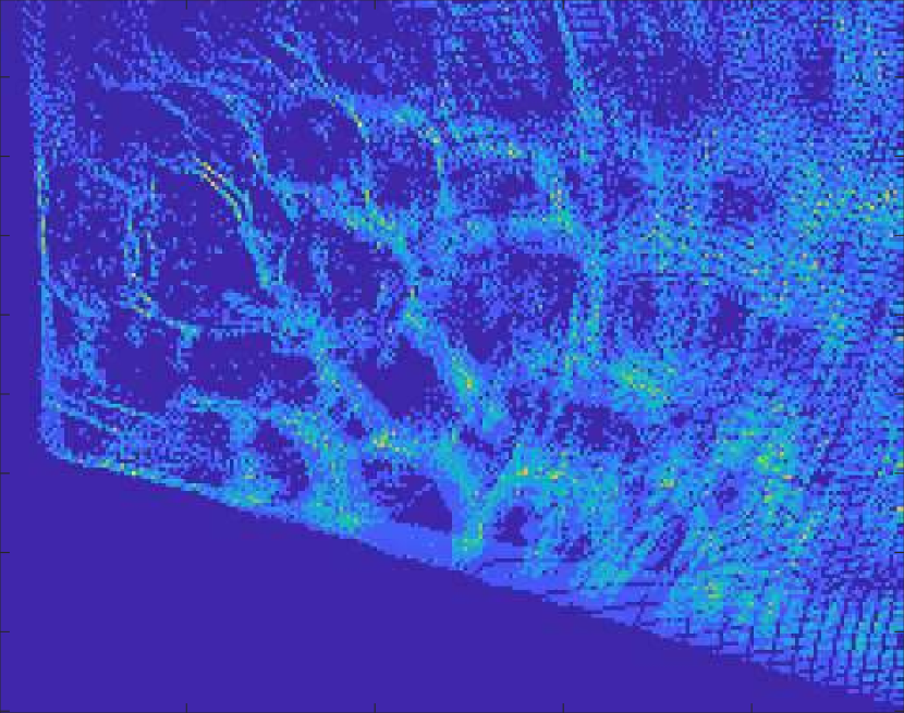
Subseq 4
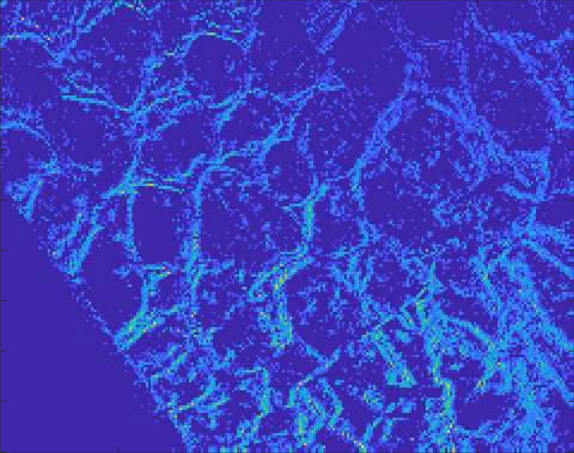
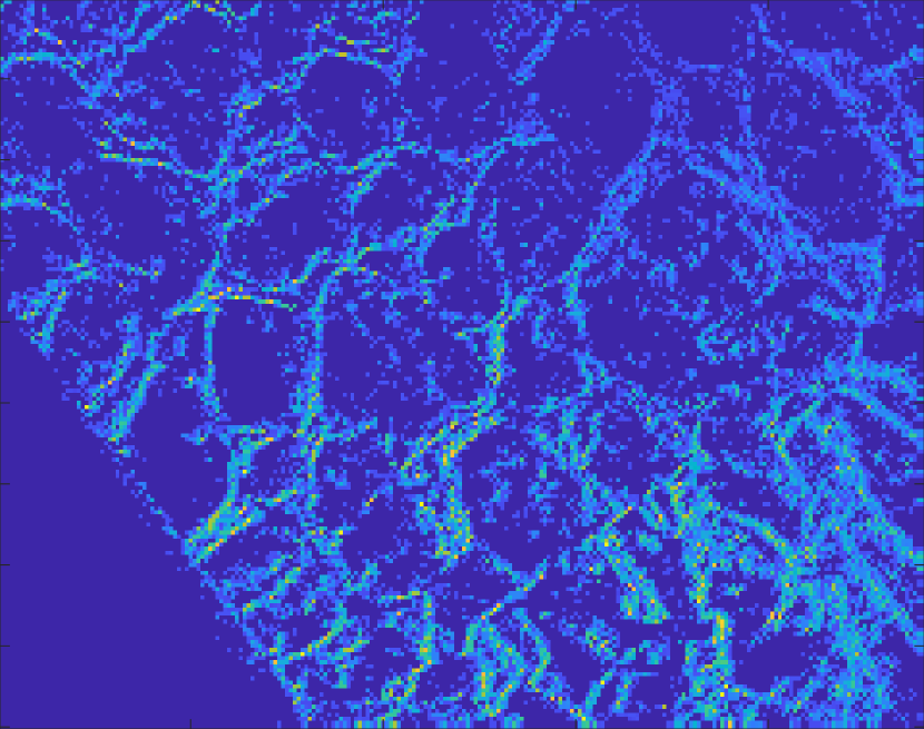
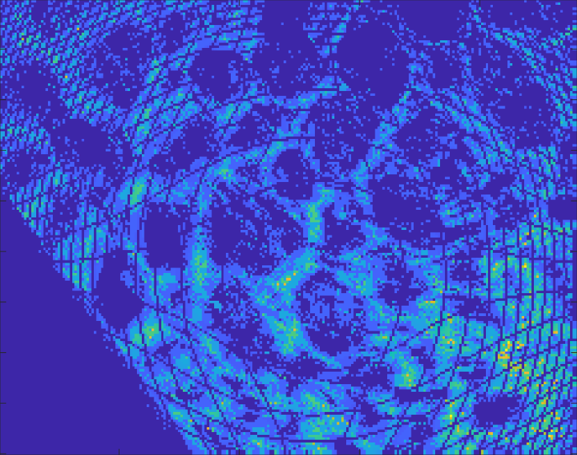
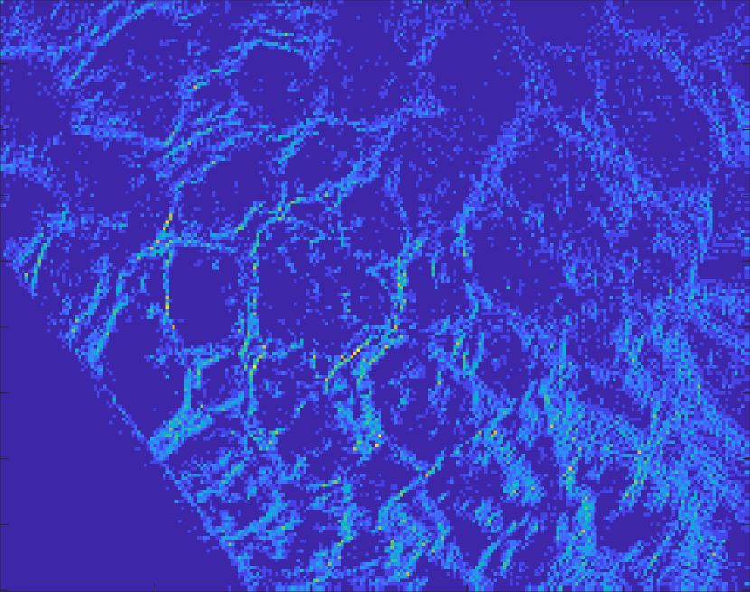
Subseq 5

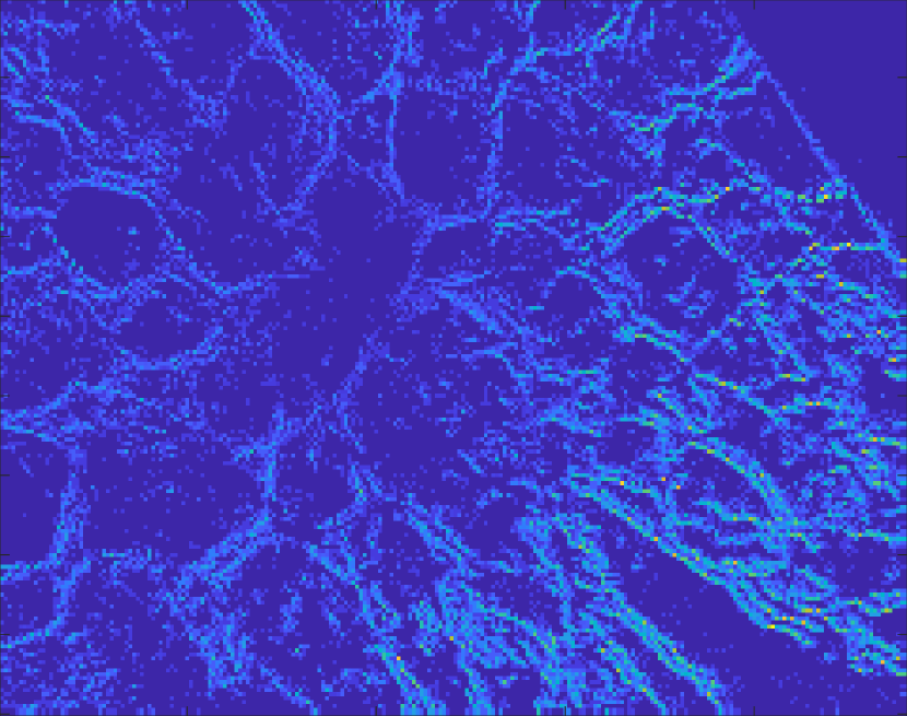
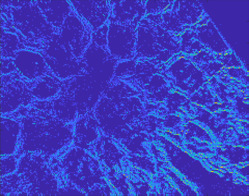
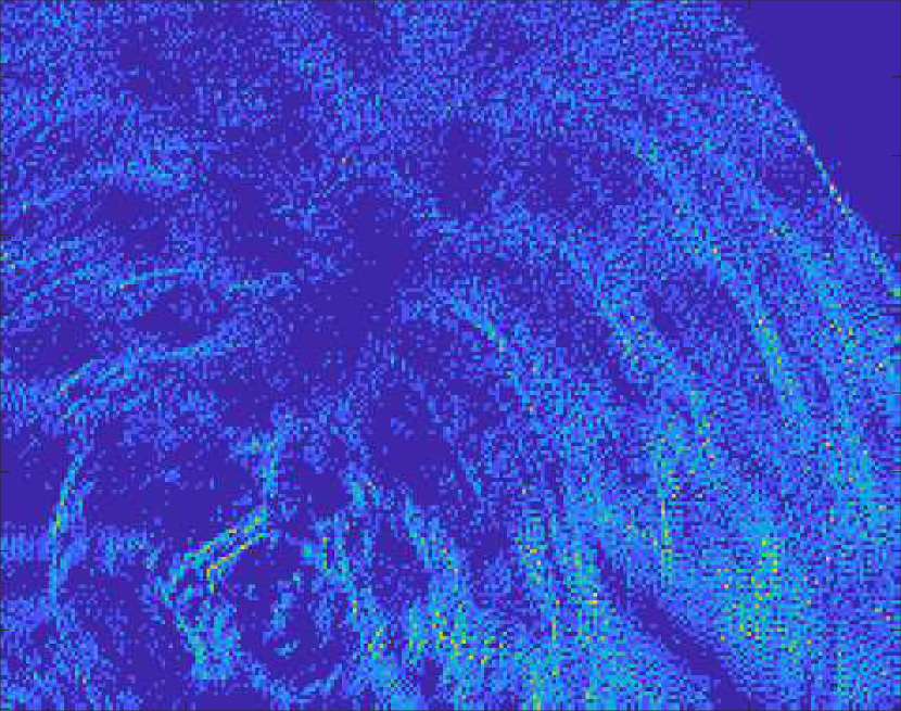
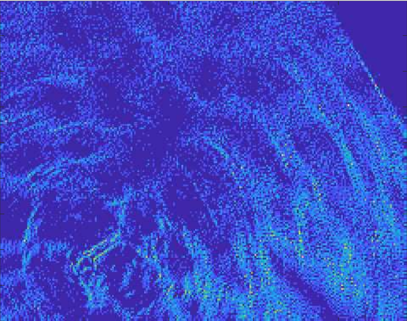
Figure 8: Qualitative results (motion compensated event images) for poster.

References

- [1] http://en.wikipedia.org/w/index.php?title=Exponential%20map%20(Lie%20theory)&oldid=925866493.
- [2] Event-based vision resources. https://github.com/uzh-rpg/event-based_vision_resources.
- [3] Jean-Charles Bazin, Hongdong Li, In So Kweon, Cédric Demonceaux, Pascal Vasseur, and Katsushi Ikeuchi. A branch-and-bound approach to correspondence and grouping problems. IEEE transactions on pattern analysis and machine intelligence, 35(7):1565–1576, 2012.
- [4] Christian Brandli, Raphael Berner, Minhao Yang, Shih-Chii Liu, and Tobi Delbruck. A 240 180 130 db 3 s latency global shutter spatiotemporal vision sensor. IEEE Journal of Solid-State Circuits, 49(10):2333–2341, 2014.
- [5] Nathan A Carr, Jared Hoberock, Keenan Crane, and John C Hart. Fast gpu ray tracing of dynamic meshes using geometry images. In Proceedings of Graphics Interface 2006, pages 203–209. Canadian Information Processing Society, 2006.
- [6] Andrea Censi and Davide Scaramuzza. Low-latency event-based visual odometry. In 2014 IEEE International Conference on Robotics and Automation (ICRA), pages 703–710. IEEE, 2014.
- [7] Tat-Jun Chin and Samya Bagchi. Event-based star tracking via multiresolution progressive hough transforms. arXiv preprint arXiv:1906.07866, 2019.
- [8] Tat-Jun Chin, Samya Bagchi, Anders Eriksson, and Andre van Schaik. Star tracking using an event camera. In Proceedings of the IEEE Conference on Computer Vision and Pattern Recognition Workshops, pages 0–0, 2019.
- [9] Rolf Clackdoyle and Catherine Mennessier. Centers and centroids of the cone-beam projection of a ball. Physics in Medicine & Biology, 56(23):7371, 2011.
- [10] Tobi Delbruck and Manuel Lang. Robotic goalie with 3 ms reaction time at 4% cpu load using event-based dynamic vision sensor. Frontiers in neuroscience, 7:223, 2013.
- [11] James D Foley, Foley Dan Van, Andries Van Dam, Steven K Feiner, John F Hughes, J Hughes, and Edward Angel. Computer graphics: principles and practice, volume 12110. Addison-Wesley Professional, 1996.
- [12] Guillermo Gallego, Mathias Gehrig, and Davide Scaramuzza. Focus is all you need: Loss functions for event-based vision. In Proceedings of the IEEE Conference on Computer Vision and Pattern Recognition, pages 12280–12289, 2019.
- [13] Guillermo Gallego, Jon EA Lund, Elias Mueggler, Henri Rebecq, Tobi Delbruck, and Davide Scaramuzza. Event-based, 6-dof camera tracking from photometric depth maps. IEEE transactions on pattern analysis and machine intelligence, 40(10):2402–2412, 2017.
- [14] Guillermo Gallego, Henri Rebecq, and Davide Scaramuzza. A unifying contrast maximization framework for event cameras, with applications to motion, depth, and optical flow estimation. In Proceedings of the IEEE Conference on Computer Vision and Pattern Recognition, pages 3867–3876, 2018.
- [15] Guillermo Gallego and Davide Scaramuzza. Accurate angular velocity estimation with an event camera. IEEE Robotics and Automation Letters, 2(2):632–639, 2017.
- [16] Richard I Hartley and Fredrik Kahl. Global optimization through rotation space search. International Journal of Computer Vision, 82(1):64–79, 2009.
- [17] Reiner Horst and Hoang Tuy. Global optimization: deterministic approaches. Springer, 1996.
- [18] Mina A Khoei, Sio-hoi Ieng, and Ryad Benosman. Asynchronous event-based motion processing: From visual events to probabilistic sensory representation. Neural computation, 31(6):1114–1138, 2019.
- [19] Hanme Kim, Ankur Handa, Ryad Benosman, Sio-Hoi Ieng, and Andrew J Davison. Simultaneous mosaicing and tracking with an event camera. J. Solid State Circ, 43:566–576, 2008.
- [20] Hanme Kim, Stefan Leutenegger, and Andrew J Davison. Real-time 3d reconstruction and 6-dof tracking with an event camera. In European Conference on Computer Vision, pages 349–364. Springer, 2016.
- [21] Beat Kueng, Elias Mueggler, Guillermo Gallego, and Davide Scaramuzza. Low-latency visual odometry using event-based feature tracks. In 2016 IEEE/RSJ International Conference on Intelligent Robots and Systems (IROS), pages 16–23. IEEE, 2016.
- [22] Yinlong Liu, Yuan Dong, Zhijian Song, and Manning Wang. 2d-3d point set registration based on global rotation search. IEEE Transactions on Image Processing, 28(5):2599–2613, 2018.
- [23] Elias Mueggler, Basil Huber, and Davide Scaramuzza. Event-based, 6-dof pose tracking for high-speed maneuvers. In 2014 IEEE/RSJ International Conference on Intelligent Robots and Systems, pages 2761–2768. IEEE, 2014.
- [24] Elias Mueggler, Henri Rebecq, Guillermo Gallego, Tobi Delbruck, and Davide Scaramuzza. The event-camera dataset and simulator: Event-based data for pose estimation, visual odometry, and slam. The International Journal of Robotics Research, 36(2):142–149, 2017.
- [25] David Mumford. Algebraic geometry I: complex projective varieties. Springer Science & Business Media, 1995.
- [26] Jorge Nocedal and Stephen Wright. Numerical optimization. Springer Science & Business Media, 2006.
- [27] Stefan Popov, Johannes Günther, Hans-Peter Seidel, and Philipp Slusallek. Stackless kd-tree traversal for high performance gpu ray tracing. In Computer Graphics Forum, volume 26, pages 415–424. Wiley Online Library, 2007.
- [28] Bharath Ramesh, Hong Yang, Garrick Michael Orchard, Ngoc Anh Le Thi, Shihao Zhang, and Cheng Xiang. Dart: distribution aware retinal transform for event-based cameras. IEEE transactions on pattern analysis and machine intelligence, 2019.
- [29] Yusuke Sekikawa, Kosuke Hara, and Hideo Saito. Eventnet: Asynchronous recursive event processing. In Proceedings of the IEEE Conference on Computer Vision and Pattern Recognition, pages 3887–3896, 2019.
- [30] Timo Stoffregen, Guillermo Gallego, Tom Drummond, Lindsay Kleeman, and Davide Scaramuzza. Event-based motion segmentation by motion compensation. arXiv preprint arXiv:1904.01293, 2019.
- [31] Timo Stoffregen and Lindsay Kleeman. Event cameras, contrast maximization and reward functions: An analysis. In The IEEE Conference on Computer Vision and Pattern Recognition (CVPR), June 2019.
- [32] Jerry R Van Aken. An efficient ellipse-drawing algorithm. IEEE Computer Graphics and Applications, 4(9):24–35, 1984.
- [33] Antoni Rosinol Vidal, Henri Rebecq, Timo Horstschaefer, and Davide Scaramuzza. Ultimate slam? combining events, images, and imu for robust visual slam in hdr and high-speed scenarios. IEEE Robotics and Automation Letters, 3(2):994–1001, 2018.
- [34] David Weikersdorfer, David B Adrian, Daniel Cremers, and Jörg Conradt. Event-based 3d slam with a depth-augmented dynamic vision sensor. In 2014 IEEE International Conference on Robotics and Automation (ICRA), pages 359–364. IEEE, 2014.
- [35] Chengxi Ye. Learning of dense optical flow, motion and depth, from sparse event cameras. PhD thesis, 2019.
- [36] Zhengyou Zhang. A flexible new technique for camera calibration. IEEE Transactions on pattern analysis and machine intelligence, 22, 2000.
- [37] Alex Zihao Zhu, Liangzhe Yuan, Kenneth Chaney, and Kostas Daniilidis. Ev-flownet: Self-supervised optical flow estimation for event-based cameras. arXiv preprint arXiv:1802.06898, 2018.
- [38] Alex Zihao Zhu, Liangzhe Yuan, Kenneth Chaney, and Kostas Daniilidis. Unsupervised event-based learning of optical flow, depth, and egomotion. In Proceedings of the IEEE Conference on Computer Vision and Pattern Recognition, pages 989–997, 2019.