Algorithms for Subpath Convex Hull Queries and Ray-Shooting Among Segments

Abstract

In this paper, we first consider the subpath convex hull query problem: Given a simple path $\pi$ of $n$ vertices, preprocess it so that the convex hull of any query subpath of $\pi$ can be quickly obtained. Previously, Guibas, Hershberger, and Snoeyink [SODA 90’] proposed a data structure of $O(n)$ space and $O(\log n\log\log n)$ query time; reducing the query time to $O(\log n)$ increases the space to $O(n\log\log n)$. We present an improved result that uses $O(n)$ space while achieving $O(\log n)$ query time. Like the previous work, our query algorithm returns a compact interval tree representing the convex hull so that standard binary-search-based queries on the hull can be performed in $O(\log n)$ time each. The preprocessing time of our data structure is $O(n)$, after the vertices of $\pi$ are sorted by $x$-coordinate. As the subpath convex hull query problem has many applications, our new result leads to improvements for several other problems.

In particular, with the help of the above result, along with other techniques, we present new algorithms for the ray-shooting problem among segments. Given a set of $n$ (possibly intersecting) line segments in the plane, preprocess it so that the first segment hit by a query ray can be quickly found. We give a data structure of $O(n\log n)$ space that can answer each query in $(\sqrt{n}\log n)$ time. If the segments are nonintersecting or if the segments are lines, then the space can be reduced to $O(n)$. As a by-product, given a set of $n$ (possibly intersecting) segments in the plane, we build a data structure of $O(n)$ space that can determine whether a query line intersects a segment in $O(\sqrt{n}\log n)$ time. The preprocessing time is $O(n^{1.5})$ for all four problems, which can be reduced to $O(n\log n)$ time by a randomized algorithm so that the query time is bounded by $O(\sqrt{n}\log n)$ with high probability. All these are classical problems that have been studied extensively. Previously data structures of $\widetilde{O}(\sqrt{n})$ query time were known in early 1990s; nearly no progress has been made for more than two decades. For all these problems, our new results provide improvements by reducing the space of the data structures by at least a logarithmic factor while the preprocessing and query times are the same as before or even better.

1 Introduction

In this paper, we first consider the subpath convex hull query problem. Let $\pi$ be a simple path of $n$ vertices in the plane. A subpath hull query specifies two vertices of $\pi$ and asks for the convex hull of the subpath between the two vertices. The goal is to preprocess $\pi$ so that the subpath hull queries can be answered quickly. Ideally, the query should return a representation of the convex hull so that standard queries on the hull can be performed in logarithmic time.

The problem has been studied by Guibas, Hershberger, and Snoeyink[25], who proposed a method of using compact interval trees. After $O(n\log n)$ time preprocessing, Guibas et al. [25] built a data structure of $O(n)$ space that can answer each query in $O(\log n\log\log n)$ time. Their query algorithm returns a compact interval tree that represents the convex hull so that all binary-search-based queries on the hull can be performed in $O(\log n)$ time each. The queries on the hull include (but are not limited to) the following: find the most extreme vertex of the convex hull along a query direction; find the intersection between a query line and the convex hull; find the common tangents from a query point to the convex hull; determine whether a query point is inside the convex hull, etc. Guibas et al. [25] reduced the subpath hull query time to $O(\log n)$ but the space becomes $O(n\log\log n)$. A trade-off was also made with $O(\log n\log^{*}n)$ query time and $O(n\log^{*}n)$ space [25].

As compact interval trees are quite amenable, the results of Guibas et al. [25] have found many applications, e.g., [5, 16, 14, 15, 17, 18, 36]. Clearly, there is still some room for further improvement on the results of Guibas et al. [25]; the ultimate goal might be an $O(n)$ space data structure with $O(\log n)$ query time. In this paper, we achieve this goal. The preprocessing time of our data structure is $O(n)$, after the vertices of $\pi$ are sorted by $x$-coordinate. Like the results of Guibas et al. [25], our query algorithm also returns a compact interval tree that can support logarithmic time queries for all binary-search-based queries on the convex hull of the query subpath; the edges of the convex hull can be retrieved in time linear in the number of vertices of the convex hull. Note that like those in [25] our results are for the random access machine (RAM) model.

With our new result, previous applications that use the results of Guibas et al. [25] can now be improved accordingly. We will demonstrate some of them, including the problem of enclosing polygons by two minimum area rectangles [6, 5], computing a guarding set for simple polygons in wireless location [17], computing optimal time-convex hulls [18], $L_{1}$ top-$k$ weighted sum aggregate nearest and farthest neighbor searching [36], etc. For all these problems, we reduce the space of their algorithms by a $\log\log n$ factor while the time complexities are the same as before or even better.

We should point out that Wagener [35] proposed a parallel algorithm for computing a data structure, called bridge tree, for representing the convex hull of a simple path $\pi$. If using one processor, for any query subpath of $\pi$, Wagener [35] showed that the bridge tree can be used to answer decomposable queries on the convex hull of the query subpath in logarithmic time each. Wagener [35] claimed that some non-decomposable queries can also be handled; however no details were provided. In contrast, our approach returns a compact interval tree that is more amenable (indeed, the bridge trees [35] were mainly designed for parallel processing) and can support both decomposable and non-decomposable queries. In addition, if one wants to output the convex hull of the query subpath, our approach can do so in time linear in the number of the vertices of the convex hull while the method of Wagener [35] needs $O(n)$ time.

1.1 Ray-Shooting

With the help of our subpath hull query data structure and many other new techniques, we present improved results for several classical ray-shooting problems. These problems have been studied extensively. Previously, data structures of $\widetilde{O}(\sqrt{n})$ query time and near-linear space were known in early 1990s; nearly no progress has been made for over two decades. Our new results reduce the space by at least a logarithmic factor while still achieving the same or even better preprocessing and query times.

In the following, we use a triple $(T(n),S(n),Q(n))$ to represent the complexity of a data structure, where $T(n)$ is the preprocessing time, $S(n)$ is the space, and $Q(n)$ is the query time. We will confine the discussion of the previous work to data structures of linear or near-linear space. Refer to Table 1 for a summary. Throughout the paper, we use $\delta$ to refer to an arbitrarily small positive constant.

Ray-shooting among lines.

Given a set of $n$ lines in the plane, the problem is to build a data structure so that the first line hit by a query ray can be quickly found.

Bar-Yehuda and Fogel [4] gave a data structure of complexity $O(n^{1.5},n\log^{2}n,\sqrt{n}\log n)$. Cheng and Janardan [16] gave a data structure of complexity $O(n^{1.5}\log^{2}n,n\log n,\sqrt{n}\log n)$. Agarwal and Sharir [2] developed a data structure of complexity $O(n\log n,n\log n,n^{1/2+\delta})$.

By using our subpath hull query data structure and a result from Chazelle and Guibas [11], we present a new data structure of complexity $O(n^{1.5},n,\sqrt{n}\log n)$. This is the first time that this problem is solved in $\widetilde{O}(\sqrt{n})$ time while using only $O(n)$ space.

In addition, we also consider a more general first-$k$-hits query, i.e., given a query ray and an integer $k$, report the first $k$ lines hit by the ray. This problem was studied by Bar-Yehuda and Fogel [4], who gave a data structure of complexity $O(n^{1.5},n\log^{2}n,\sqrt{n}\log n+k\log^{2}n)$. Our new result is a data structure of complexity $O(n^{1.5},n,\sqrt{n}\log n+k\log n)$.

Intersection detection.

Given a set of $n$ line segments in the plane, the problem is to build a data structure to determine whether a query line intersects at least one segment.

Cheng and Janardan [16] gave a data structure of complexity $O(n^{1.5}\log^{2}n,n\log n,\sqrt{n}\log n)$. By adapting the interval partition trees of Overmars et al. [34] (which relies on the conjugation trees of Edelsbrunner and Welzl [23]) to the partition trees of Matoušek [31, 32], we obtain a data structure of complexity $O(n^{1.5},n,\sqrt{n}\log n)$. To this end, we have to use Matoušek’s techniques in both [31] and [32], and modify them in a not-so-trivial mannar.

Ray-shooting among segments.

Given a set of $n$ (possibly intersecting) line segments in the plane, the problem is to build a data structure to find the first segment hit by a query ray.

Overmars et al. [34] gave a data structure of complexity $O(n\alpha(n)\log^{3}n,n\log^{2}n,n^{0.695}\log n)$, where $\alpha(n)$ is the inverse Ackermann’s function. Guibas et al. [26] presented a data structure of complexity $O(n\alpha(n)\log^{3}n,n\alpha(n),n^{2/3+\delta})$. Agarwal [1] gave a data structure of complexity $O(n^{1.5}\log^{4.33}n,n\alpha(n)\log^{4}n,\sqrt{n\alpha(n)}\log^{2}n)$. Bar-Yehuda and Fogel [4] gave a data structure of complexity $O((n\alpha(n))^{1.5},n\alpha(n)\log^{2}n,\sqrt{n\alpha(n)}\log n)$. Cheng and Janardan [16] developed a data structure of complexity $O(n^{1.5}\log^{2}n,n\log^{2}n,\sqrt{n}\log n)$. Agarwal and Sharir [2] proposed a data structure of complexity $O(n\log^{2}n,n\log^{2}n,n^{0.5+\delta})$. Chan’s randomized techniques [8] yielded a data structure of complexity $O(n\log^{3}n,n\log^{2}n,\sqrt{n}\log^{2}n)$, where the query time is expected.

Cheng and Janardan’s algorithm [16] relies on their results for the ray-shooting problem among lines and the intersection detection problem. Following their algorithmic scheme and using our above new results for these two problems, we obtain a data structure for the ray-shooting problem among segments with complexity $O(n^{1.5},n\log n,\sqrt{n}\log n)$. This is the first data structure of $\widetilde{O}(\sqrt{n})$ query time that uses only $O(n\log n)$ space.

If the segments are nonintersecting, then better results exist. Overmars et al. [34] gave a data structure of complexity $O(n\log n,n,n^{0.695}\log n)$. Agarwal [1] presented a data structure of complexity $O(n^{1.5}\log^{4.33}n,n\alpha(n)\log^{3}n,\sqrt{n}\log^{2}n)$. Bar-Yehuda and Fogel [4] proposed a data structure of complexity $O(n^{1.5},n\log n,\sqrt{n}\log n)$. Our new data structure has complexity $O(n^{1.5},n,\sqrt{n}\log n)$. This is the first data structure of $\widetilde{O}(\sqrt{n})$ query time that uses only $O(n)$ space. Note that if the segments form the boundary of a simple polygon, then there exist data structures of complexity $O(n,n,\log n)$ [10, 12, 28].

	Preprocessing time	Space	Query time	Source
42.5cmRay-shooting among lines	$n^{1.5}$	$n\log^{2}n$	$\sqrt{n}\log n$	BF[4]
	$n^{1.5}\log^{2}n$	$n\log n$	$\sqrt{n}\log n$	CJ[16]
	$n\log n$	$n\log n$	$n^{0.5+\delta}$	AS[2]
	$n^{1.5}$	$n$	$\sqrt{n}\log n$	this paper
	$n\log n$	$n$	$\sqrt{n}\log n$ *	this paper
32.5cmIntersection detection	$n^{1.5}\log^{2}n$	$n\log n$	$\sqrt{n}\log n$	CJ[16]
	$n^{1.5}$	$n$	$\sqrt{n}\log n$	this paper
	$n\log n$	$n$	$\sqrt{n}\log n$ *	this paper
92.5cmRay-shooting among intersecting segments	$n\alpha(n)\log^{3}n$	$n\log^{2}n$	$n^{0.695}\log n$	OSS[34]
	$n\alpha(n)\log^{3}n$	$n\alpha(n)$	$n^{2/3+\delta}$	GOS[26]
	$n^{1.5}\log^{4.33}n$	$n\alpha(n)\log^{4}n$	$\sqrt{n\alpha(n)}\log^{2}n$	A [1]
	$(n\alpha(n))^{1.5}$	$n\alpha(n)\log^{2}n$	$\sqrt{n\alpha(n)}\log n$	BF [4]
	$n^{1.5}\log^{2}n$	$n\log^{2}n$	$\sqrt{n}\log n$	CJ[16]
	$n\log^{2}n$	$n\log^{2}n$	$n^{0.5+\delta}$	AS [2]
	$n\log^{3}n$	$n\log^{2}n$	$\sqrt{n}\log^{2}n$ *	C [8]
	$n^{1.5}$	$n\log n$	$\sqrt{n}\log n$	this paper
	$n\log^{2}n$	$n\log n$	$\sqrt{n}\log n$ *	this paper
52.5cmRay-shooting among nonintersecting segments	$n\log n$	$n$	$n^{0.695}\log n$	OSS [34]
	$n^{1.5}\log^{4.33}n$	$n\alpha(n)\log^{3}n$	$\sqrt{n}\log^{2}n$	A [1]
	$n^{1.5}$	$n\log n$	$\sqrt{n}\log n$	BF [4]
	$n^{1.5}$	$n$	$\sqrt{n}\log n$	this paper
	$n\log n$	$n$	$\sqrt{n}\log n$ *	this paper

Table 1: Summary of the results. The big-$O$ notation is omitted. $\delta$ can be any small positive constant. The results marked with * hold with high probability (except that the result of Chan [8] is expected).

Randomized results.

Using Chan’s randomized techniques [8], the preprocessing time of all our above results can be reduced to $O(n\log n)$ (except $O(n\log^{2}n)$ time for the ray-shooting problem among intersecting segments), while the same query time complexities hold with high probability (i.e., probability at least $1-1/n^{c}$ for any large constant $c$).

Outline.

The rest of the paper is organized as follows. In Section 2 we review some previous work of the subpath hull query problem; Section 3 presents our new data structure for the problem. Section 4 is concerned with the ray-shooting problem. Other applications of the our subpath hull query result are discussed in Section 5.

2 Preliminaries

Let $p_{1},\ldots,p_{n}$ be the vertices of a simple path $\pi$ ordered along $\pi$. For any two indices $i$ and $j$ with $1\leq i\leq j\leq n$, we use $\pi(i,j)$ to refer to the subpath of $\pi$ from $p_{i}$ to $p_{j}$. Given a pair $(i,j)$ of indices with $1\leq i\leq j\leq n$, the subpath hull query asks for the convex hull of $\pi(i,j)$.

The convex hull of a simple path can be found in linear time, e.g., [24, 33]. Note that the convex hull of a simple path is the same as the convex hull of its vertices. For this reason, in our discussion a subpath $\pi^{\prime}$ of $\pi$ actually refers to its vertex set. For each subpath $\pi^{\prime}$ of $\pi$, we use $|\pi^{\prime}|$ to denote the number of vertices of $\pi^{\prime}$; we consider the endpoint of $\pi^{\prime}$ that is closer to $p_{1}$ in $\pi$ as the first vertex of $\pi^{\prime}$ while the other endpoint is the last vertex of $\pi^{\prime}$. So $p_{i}$ is the first vertex and $p_{j}$ is the last vertex of $\pi(i,j)$.

For any set $P$ of points in the plane, let $H(P)$ denote the convex hull of $P$. Denote by $H_{U}(P)$ and $H_{L}(P)$ the upper and lower hulls, respectively.

Interval trees.

Let $S$ be a set of $n$ points in the plane. The interval tree $T(S)$ is a complete binary tree whose leaves from left to right correspond to the points of $S$ sorted from left to right. Each internal node corresponds to the interval between the rightmost leaf in its left subtree and the leftmost leaf in its right subtree. We say that a segment joining two points of $S$ spans an internal node $v$ if $v$ is between the two endpoints of the segment in the symmetric order of the nodes of $T(S)$ (or equivalently, the projection of the interval of $v$ on the $x$-axis is contained in the projection of the segment on the $x$-axis).

We store each edge $e$ of the upper hull $H_{U}(S)$ at the highest node of $T(S)$ that $e$ spans (e.g., see Fig. 1). By also storing the edges of the lower hull $H_{L}(S)$ in $T(S)$ in the same way, we can answer all standard binary-search-based queries on the convex hull $H(S)$ in $O(\log n)$ time, by following a path from the root of $T(S)$ to a leaf [25]. The main idea is that the edge of $H_{U}(S)$ (resp., $H_{L}(S)$) spanning a node $v$ of $T(S)$ is stored either at $v$ or at one of $v$’s ancestors and only at most two ancestors closest to $v$ (one to the left and the other to the right of $v$) need to be remembered during the search (see Lemma 4.1 of [25] for details).

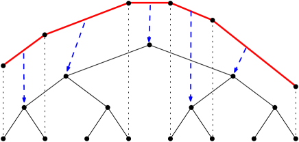
Figure 1: Illustrating an interval tree that stores upper hull edges: the (blue) dashed lines with arrows indicate where edges are stored.

Compact interval trees.

As the size of $T(S)$ is $\Theta(n)$ while $|H(S)|$ may be much smaller than $n$, where $|H(S)|$ is the number of edges of $H(S)$, using $T(S)$ to store $H(S)$ may not be space-efficient. Guibas et al. [25] proposed to use a compact interval tree $T_{U}(S)$ of $O(|H_{U}(S)|)$ size to store $H_{U}(S)$, as follows. In $T(S)$, a node $v$ is empty if it does not store an edge of $H_{U}(S)$; otherwise it is full. It was shown in [25] that if two nodes of $T(S)$ are full, then their lowest common ancestor is also full. We remove empty nodes from $T(S)$ by relinking the tree to make each full node the child of its nearest full ancestor. Let $T_{U}(S)$ be the new tree and we still use $T(S)$ to refer to the original interval tree without storing any hull edges. Each node of $T_{U}(S)$ stores exactly one edge of $H_{U}(S)$, and thus $T_{U}(S)$ has $|H_{U}(S)|$ nodes. After $O(n)$ time preprocessing on $T(S)$ (specifically, build a lowest common ancestor query data structure [7, 27], with constant query time), $T_{U}(S)$ can be computed from $H_{U}(S)$ in $O(|H_{U}(S)|)$ time (see Lemma 4.4 in [25]). Similarly, we use a compact interval tree $T_{L}(S)$ of $|H_{L}(S)|$ nodes to store $H_{L}(S)$. Then, using the three trees $T_{U}(S)$, $T_{L}(S)$, and $T(S)$, all standard binary-search-based queries on $H(S)$ can be answered in $O(\log n)$ time. The main idea is that the algorithm walks down through the compact interval trees while keeping track of the corresponding position in $T(S)$ (see Lemma 4.3 [25] for details). We call $T(S)$ a reference tree. In addition, using $T_{U}(S)$ and $T_{L}(S)$, $H(S)$ can be output in $O(|H(S)|)$ time.

As discussed above, to represent $H(S)$, we need two compact interval trees, one for $H_{U}(S)$ and the other for $H_{L}(S)$. To make our discussion more concise, we will simply say “the compact interval tree” for $S$ and use $T^{+}(S)$ to refer to it, which actually includes two trees.

Compact interval trees for $\boldsymbol{\pi}$.

Consider two consecutive subpaths $\pi_{1}$ and $\pi_{2}$ of $\pi$. Suppose their compact interval trees $T^{+}(\pi_{1})$ and $T^{+}(\pi_{2})$ as well as the interval tree $T(\pi)$ of $\pi$ are available. It is known that the convex hulls of two consecutive subpaths of a simple path have at most two common tangents [11]. Hence, $H(\pi_{1})$ and $H(\pi_{2})$ have at most two common tangents. By using the path-copying method of persistent data structures [20], Guibas et al. [25] obtained the following result.

Lemma 1.

(Guibas et al. [25]) Without altering $T^{+}(\pi_{1})$ and $T^{+}(\pi_{2})$, the compact interval tree $T^{+}(\pi_{1}\cup\pi_{2})$ can be produced (the root of the tree will be returned) in $O(\log n)$ time and $O(\log n)$ additional space.

Lemma 2.

(Guibas et al. [25]) Given the interval tree $T(\pi)$, with $O(n)$ time preprocessing, we can compute $T^{+}(\pi^{\prime})$ for any subpath $\pi^{\prime}$ of $\pi$ in $O(|\pi^{\prime}|)$ time.

Proof.

We preprocess $T(\pi)$ in the same way as preprocessing $T(S)$ discussed before (i.e., build a lowest common ancestor query data structure [7, 27], with constant query time). For any subpath $\pi^{\prime}$ of $\pi$, we first compute its convex hull $H(\pi^{\prime})$ in $O(|\pi^{\prime}|)$ time [24, 33]. Then, as discussed before, $T^{+}(\pi^{\prime})$ can be constructed in $O(|H(\pi^{\prime})|)$ time (Lemma 4.4 in [25]). ∎

3 Subpath Convex Hull Queries

In this section, we present our new data structure for subpath hull queries. We first compute a sorted list of all vertices of $\pi$ by $x$-coordinate. As will be seen later, the rest of the preprocessing of our data structure takes $O(n)$ time in total.

3.1 A decomposition tree

After having the interval tree $T(\pi)$, we construct a decomposition tree $\Psi(\pi)$, which is a segment tree on the vertices of $\pi$ following their order along $\pi$. Specifically, $\Psi(\pi)$ is a complete binary tree with $n$ leaves corresponding to the vertices of $\pi$ in order along $\pi$. Each internal node $v$ of $\Psi(\pi)$ corresponds to the subpath $\pi(a_{v},b_{v})$, where $a_{v}$ (resp., $b_{v}$) is defined to be the index of the vertex of $\pi$ corresponding to the leftmost (resp., rightmost) leaf of the subtree of $\Psi(\pi)$ rooted at $v$; we call $\pi(a_{v},b_{v})$ a canonical subpath of $\pi$ and use $\pi(v)$ to denote it.

Next, we remove some nodes in the lower part of $\Psi(\pi)$, as follows. For each node $v$ whose canonical path has at most $\log^{2}n$ vertices and whose parent canonical subpath has more than $\log^{2}n$ vertices, we remove both the left and the right subtrees of $v$ from $\Psi(\pi)$ but explicitly store $\pi(v)$ at $v$, after which $v$ becomes a leaf of the new tree. From now on we use $\Psi(\pi)$ to refer to the new tree. It is not difficult to see that $\Psi(\pi)$ now has $O(n/\log^{2}n)$ nodes.

We then compute compact interval trees $T^{+}(\pi(v))$ for all nodes $v$ of $\Psi(\pi)$ in a bottom-up manner. Specifically, if $v$ is a leaf, then $\pi(v)$ has at most $\log^{2}n$ vertices, and we compute $T^{+}(\pi(v))$ from scratch, which takes $O(\log^{2}n)$ time by Lemma 2. If $v$ is not a leaf, then $T^{+}(\pi(v))$ can be obtained by merging the two compact interval trees of its children, which takes $O(\log n)$ time by Lemma 1. In this way, computing compact interval trees for all nodes of $\Psi(\pi)$ takes $O(n)$ time in total, for $\Psi(\pi)$ has $O(n/\log^{2}n)$ nodes.

3.2 A preliminary query algorithm

Consider a subpath hull query $(i,j)$. We first present an $O(\log^{2}n)$ time query algorithm using $\Psi(\pi)$ and then reduce the time to $O(\log n)$. Depending on whether the two vertices $p_{i}$ and $p_{j}$ are in the same canonical subpath of a leaf of $\Psi(\pi)$, there are two cases.

Case 1.

If yes, let $v$ be the leaf. Then, $\pi(i,j)$ is a subpath of $\pi(v)$ and thus has at most $\log^{2}n$ vertices. We compute $T^{+}(\pi(i,j))$ from scratch in $O(\log^{2}n)$ time by Lemma 2.

Case 2.

Otherwise, let $v$ be the leaf of $\Psi(\pi)$ whose canonical subpath contains $p_{i}$ and $u$ the leaf whose canonical subpath contains $p_{j}$. Let $w$ be the lowest common ancestor of $u$ and $v$. As in [25], we partition $\pi(i,j)$ into two subpaths $\pi(i,k)$ and $\pi(k+1,j)$, where $k=b_{w^{\prime}}$ with $w^{\prime}$ being the left child of $w$ (recall the definition of $b_{w^{\prime}}$ given before). We will compute the compact interval trees for the two subpaths separately, and then merge them to obtain $T^{+}(\pi(i,j))$ in additional $O(\log n)$ time by Lemma 1. We only discuss how to compute $T^{+}(\pi(i,k))$, for the other tree can be computed likewise.

We further partition $\pi(i,k)$ into two subpaths $\pi(i,b_{v})$ and $\pi(b_{v}+1,k)$. We will compute the compact interval trees for them separately and then merge the two trees to obtain $T^{+}(\pi(i,k))$.

For computing $T^{+}(\pi(i,b_{v}))$, as $\pi(i,b_{v})$ is a subpath of $\pi(v)$, it has at most $\log^{2}n$ vertices. Hence, we can compute $T^{+}(\pi(i,b_{v}))$ from scratch in $O(\log^{2}n)$ time.

For computing $T^{+}(\pi(b_{v}+1,k))$, observe that $\pi(b_{v}+1,k)$ is the concatenation of the canonical subpaths of $O(\log n)$ nodes of $\Psi(\pi)$; precisely, these nodes are the right children of their parents that are in the path of $\Psi(\pi)$ from $v$’s parent to $w^{\prime}$ and these nodes themselves are not on the path. Since the compact interval trees of these nodes are already available due to the preprocessing, we can produce $T^{+}(\pi(b_{v}+1,k))$ in $O(\log^{2}n)$ time by merging these trees.

In summary, we can compute $T^{+}(\pi(i,j))$ in $O(\log^{2}n)$ time in either case.

3.3 Reducing the query time to $O(\log n)$

In what follows, we reduce the query time to $O(\log n)$, with additional preprocessing (but still $O(n)$).

To reduce the time for Case 1, we perform the following preprocessing. For each leaf $v$ of $\Psi(\pi)$, we preprocess the path $\pi(v)$ in the same way as above for preprocessing $\pi$. This means that we construct an interval tree $T(\pi(v))$ as well as a decomposition tree $\Psi(\pi(v))$ for the subpath $\pi(v)$. To answer a query for Case 1, we instead use $\Psi(\pi(v))$ (and use $T(\pi(v))$ as the reference tree). The query time becomes $O(\log^{2}\log n)$ as $|\pi(v)|\leq\log^{2}n$. Note that to construct $T(\pi(v))$ and $\Psi(\pi(v))$ in $O(|\pi(v)|)$ time, we need to sort all vertices of $\pi(v)$ by $x$-coordinate in $O(|\pi(v)|)$ time. Recall that we already have a sorted list of all vertices of $\pi$, from which we can obtain sorted lists for $\pi(v)$ for all leaves $v$ of $\Psi(\pi)$ in $O(n)$ time altogether. Hence, the preprocessing for $\pi(v)$ for all leaves $v$ of $\Psi(\pi)$ takes $O(n)$ time.

We proceed to Case 2. To reduce the query time to $O(\log n)$, we will discuss how to perform additional preprocessing so that $T^{+}(\pi(i,k))$ can be computed in $O(\log n)$ time. Computing $T^{+}(\pi(k+1,j))$ can be done in $O(\log n)$ time similarly. Finally we can merge the two trees to obtain $T^{+}(\pi(i,j))$ in additional $O(\log n)$ time by Lemma 1.

To compute $T^{+}(\pi(i,k))$ in $O(\log n)$ time, according to our algorithm it suffices to compute both $T^{+}(i,b_{v})$ and $T^{+}(b_{v}+1,k)$ in $O(\log n)$ time. We discuss $T^{+}(i,b_{v})$ first.

Dealing with $\boldsymbol{T^{+}(\pi(i,b_{v}))}$.

To compute $T^{+}(i,b_{v})$ in $O(\log n)$ time, we preform the following additional preprocessing. For each leaf $v$ of $\Psi(\pi)$, recall that $|\pi(v)|\leq\log^{2}n$; we partition $\pi(v)$ into $t_{v}\leq\log n$ subpaths each of which contains at most $\log n$ vertices. We use $\pi_{v}(1),\pi_{v}(2),\ldots,\pi_{v}(t_{v})$ to refer to these subpaths in order along $\pi(v)$. For each subpath $\pi_{v}(i)$, we compute $T^{+}(\pi_{v}(i))$ from scratch in $O(\log n)$ time. The total time for computing all such trees is $O(\log^{2}n)$. Next, we compute compact interval trees for $t_{v}$ prefix subpaths of $\pi(v)$. Specifically, for each $t\in[1,t_{v}]$, we compute $T^{+}(\pi_{v}[1,t])$, where $\pi_{v}[1,t]$ is the concatenation of the paths $\pi_{v}(1),\pi_{v}(2),\ldots,\pi_{v}(t)$. This can be done in $O(\log^{2}n)$ time by computing $T^{+}(\pi_{v}[1,t])$ incrementally for $t=1,2,\ldots,t_{v}$ using the merge algorithm of Lemma 1. Indeed, initially $T^{+}(\pi_{v}[1,t])=T^{+}(\pi_{v}(1))$, which is already available. Then, for each $2\leq t\leq t_{v}$, $T^{+}(\pi_{v}[1,t])$ can be produced by merging $T^{+}(\pi_{v}[1,t-1])$ and $T^{+}(\pi_{v}(t))$ in $O(\log n)$ time. Similarly, we compute compact interval trees for $t_{v}$ suffix subpaths of $\pi(v)$: $T^{+}(\pi_{v}[t,t_{v}])$ for all $t=1,2,\ldots,t_{v}$, where $\pi_{v}[t,t_{v}]$ is the concatenation of the paths $\pi_{v}(t),\pi_{v}(t+1),\ldots,\pi_{v}(t_{v})$. This can be done in $O(\log^{2}n)$ time by a similar algorithm as above. Thus, the preprocessing on $v$ takes $O(\log^{2}n)$ time; the preprocessing on all leaves of $\Psi(\pi)$ takes $O(n)$ time in total.

We can now compute $T^{+}(i,b_{v})$ in $O(\log n)$ time as follows. Recall that $\pi(i,b_{v})$ is a subpath of $\pi(v)$ and $b_{v}$ is the last vertex of $\pi(v)$. We first determine the subpath $\pi_{v}(t)$ that contains $i$. Let $g$ be the last vertex of $\pi_{v}(t)$. We partition $\pi(i,b_{v})$ into two subpaths $\pi(i,g)$ and $\pi(g+1,b_{v})$, and we will compute their compact interval trees separately and then merge them to obtain $T^{+}(\pi(i,b_{v}))$. For $\pi(i,g)$, as $\pi(i,g)$ is a subpath of $\pi_{v}(t)$ and $|\pi_{v}(t)|\leq\log n$, we can compute $T^{+}(\pi(i,g))$ from scratch in $O(\log n)$ time. For $\pi(g+1,b_{v})$, observe that $\pi(g+1,b_{v})$ is exactly the suffix supath $\pi_{v}[t+1,t_{v}]$, whose compact interval tree has already been computed in the preprocessing. Hence, $T^{+}(i,b_{v})$ can be produced in $O(\log n)$ time.

Dealing with $\boldsymbol{T^{+}(\pi(b_{v}+1,k))}$.

To compute $T^{+}(b_{v}+1,k)$ in $O(\log n)$ time, we perform the following preprocessing, which was also used by Guibas et al. [25]. Recall that $\pi(b_{v}+1,k)$ is the concatenation of the canonical paths of $O(\log n)$ nodes that are right children of the nodes on the path in $\Psi(\pi)$ from $v$’s parent to the left child of $w$ (and these nodes themselves are not on the path). Hence, this sequence of nodes can be uniquely determined by the leaf-ancestor pair $(v,w)$; we use $\pi_{v,w}$ to denote the above concatenated subpath of $\pi$.

Correspondingly, in the preprocessing, for each leaf $v$ we do the following. For each ancestor $w$ of $v$, we compute the compact interval tree for the subpath $\pi_{v,w}$. As $v$ has $O(\log n)$ ancestors, computing the trees for all ancestors takes $O(\log^{2}n)$ time using the merge algorithm of Lemma 1. Hence, the total preprocessing time on $v$ is $O(\log^{2}n)$, and thus the total preprocessing time on all leaves of $\Psi(\pi)$ is $O(n)$, for $\Psi(\pi)$ has $O(n/\log^{2}n)$ leaves. Due to the above preprocessing, $T^{+}(b_{v}+1,k)$ is available during queries.

Wrapping up.

In summary, with $O(n)$ time preprocessing (excluding the time for sorting the vertices of $\pi$), we can build a data structure of $O(n)$ space that can answer each subpath hull query in $O(\log n)$ time. Comparing with the method of Guibas et al. [25], our innovation is threefold. First, we process subpaths individually to handle queries of Case 1. Second, we precompute the compact interval trees for convex hulls of the prefix and suffix subpaths of $\pi(v)$ for each leaf $v$ of $\Psi(\pi)$. Third, we use a smaller decomposition tree $\Psi(\pi)$ of only $O(n/\log^{2}n)$ nodes. The following theorem summarizes our result.

Theorem 3.1.

Given a simple path $\pi$ of $n$ vertices in the plane, after all vertices are sorted by $x$-coordinate, a data structure of $O(n)$ space can be built in $O(n)$ time so that each subpath hull query can be answered in $O(\log n)$ time. The query algorithm produces a compact interval tree representing the convex hull of the query subpath, which can support all binary-search-based operations on the convex hull in $O(\log n)$ time each. These operations include (but are not limited to) the following (let $\pi^{\prime}$ denote the query subpath and let $H(\pi^{\prime})$ be its convex hull):

1. Given a point, decide whether the point is in $H(\pi^{\prime})$.

2. Given a point outside $H(\pi^{\prime})$, find the two tangents from the point to $H(\pi^{\prime})$.

3. Given a direction, find the most extreme point of $\pi^{\prime}$ along the direction.

4. Given a line, find its intersection with $H(\pi^{\prime})$.

5. Given a convex polygon (represented in any data structure that supports binary search), decide whether it intersects $H(\pi^{\prime})$, and if not, find their common tangents (both outer and inner).

In addition, $H(\pi^{\prime})$ can be output in time linear in the number of vertices of $H(\pi^{\prime})$.

Proof 3.2.

Refer to Guibas et al. [25] for some details on how to perform operations on the convex hull $H(\pi^{\prime})$ using compact interval trees.

4 Ray-Shooting

In this section, we present our results on the ray-shooting problem. The ray-shooting problem among lines is discussed in Section 4.1. Section 4.2 is concerned with the intersection detection problem and the ray-shooting problem among segments.

4.1 Ray-shooting among lines

Given a set of $n$ lines in the plane, we wish to build a data structure so that the first line hit by a query ray can be found efficiently. The problem is usually tackled in the dual plane, e.g., [16]. Let $P$ be the set of dual points of the lines. In the dual plane, the problem is equivalent to the following: Given a query line $l_{q}$, a pivot point $q\in l_{q}$, and a rotation direction (clockwise or counterclockwise), find the first point of $P$ hit by rotating $l_{q}$ around $q$.

A spanning path $\pi(P)$ of $P$ is a polygonal path connecting all points of $P$ such that $P$ is the vertex set of the path. Hence, $\pi(P)$ corresponds to a permutation of $P$. For any line $l$ in the plane, let $\sigma(l)$ denote the number of edges of $\pi(P)$ crossed by $l$. The stabbing number of $\pi(P)$ is the largest $\sigma(l)$ of all lines $l$ in the plane. It is known that a spanning path of $P$ with stabbing number $O(\sqrt{n})$ always exists [13], which can be computed in $O(n^{1+\delta})$ time using Matoušek’s partition tree [32] (e.g., by a method in [13]). Let $\pi^{\prime}(P)$ denote such a path. Note that $\pi^{\prime}(P)$ may have self-intersections. Using $\pi^{\prime}(P)$, Edelsbrunner et al. [21] gave an algorithm that can produce another spanning path $\pi(P)$ of $P$ such that the stabbing number of $\pi(P)$ is also $O(\sqrt{n})$ and $\pi(P)$ has no self-intersections (i.e., $\pi(P)$ is a simple path); the runtime of the algorithm is $O(n^{1.5})$. Below we will use $\pi(P)$ to solve our problem.

We first build a data structure in the following lemma for $\pi(P)$.

Lemma 3.

(Chazelle and Guibas [11]) We can build a data structure of $O(n)$ size in $O(n\log n)$ time for any simple path of $n$ vertices, so that given any query line $l_{q}$, if $l_{q}$ intersects the path in $k$ edges, then these edges can be found in $O(k\log\frac{n}{k})$ time.

Then, we construct the subpath hull query data structure of Theorem 3.1 for $\pi(P)$. This finishes our preprocessing.

Given a query line $l_{q}$, along with the pivot $q$ and the rotation direction, we first use Lemma 3 to find the edges of $\pi(P)$ intersecting $l_{q}$. As the stabbing number of $\pi(P)$ is $O(\sqrt{n})$, this steps finds $O(\sqrt{n})$ edges intersecting $l_{q}$ in $O(\sqrt{n}\log n)$ time. Then, using these edges we can partition $\pi(P)$ into $O(\sqrt{n})$ subpaths each of which does not intersect $l_{q}$. For each subpath, we use our subpath hull query data structure to compute its convex hull in $O(\log n)$ time. Next, we compute the tangents from the pivot $q$ to each of these $O(\sqrt{n})$ convex hulls, in $O(\log n)$ time each by Theorem 3.1. Using these $O(\sqrt{n})$ tangents, based on the rotation direction of $l_{q}$, we can determine the first point of $P$ hit by $l_{q}$ in additional $O(\sqrt{n})$ time. Hence, the total time of the query algorithm is $O(\sqrt{n}\log n)$.

Theorem 4.1.

There exists a data structure of complexity $O(n^{1.5},n,\sqrt{n}\log n)$ for the ray-shooting problem among lines. The preprocessing time can be reduced to $O(n\log n)$ time by a randomized algorithm while the query time is bounded by $O(\sqrt{n}\log n)$ with high probability.

Proof 4.2.

We first discuss the deterministic result. The query time is $O(\sqrt{n}\log n)$, as explained above. The space is used for the data structure in Lemma 3 and the subpath hull query data structure in Theorem 3.1, which is $O(n)$. For the preprocessing time, computing $\pi(P)$ takes $O(n^{1.5})$ time. Building the data structure for Lemma 3 and the subpath hull query data structure can be done in $O(n\log n)$ time. Hence, the total preprocessing time is $O(n^{1.5})$.

For the randomized result, Chan [8] gave an $O(n\log n)$ time randomized algorithm to compute a spanning path $\pi^{\prime\prime}(P)$ for $P$ such that $\pi^{\prime\prime}(P)$ is a simple path and the stabbing number of $\pi^{\prime\prime}(P)$ is at most $O(\sqrt{n})$ with high probability. After having $\pi^{\prime\prime}(P)$, we build the data structure for Lemma 3 and the subpath hull query data structure. Hence, the preprocessing takes $O(n\log n)$ time and $O(n)$ space, and the query time is bounded by $O(\sqrt{n}\log n)$ with high probability.

Remark.

As indicated in [21], ray-shooting can be used to determine whether two query points $p$ and $q$ are in the same face of the arrangement of a set of lines. Indeed, let $\rho$ be the ray originated from $p$ towards $q$. Then, $p$ and $q$ are in the same face of the arrangement if and only if $\rho$ hits the first line after $q$.

We can extend the above algorithm to obtain the following result on the first-$k$-hit queries.

Theorem 4.3.

Given a set of $n$ lines in the plane, we can build a data structure of $O(n)$ space in $O(n^{1.5})$ time so that given a ray and an integer $k$, we can find the first $k$ lines hit by the ray in $O(\sqrt{n}\log n+k\log n)$ time. The preprocessing time can be reduced to $O(n\log n)$ while the query time is bounded by $O(\sqrt{n}\log n+k\log n)$ with high probability.

Proof 4.4.

We still work in the dual plane and use the same notation as above. In the dual plane, the problem is equivalent to finding the first $k$ points that are hit by $l_{q}$ when it is rotating around the pivot $q$ following the given direction. We perform exactly the same processing as before. Let $p_{1},p_{2},\ldots,p_{n}$ be the points of $P$ ordered along $\pi(P)$.

Figure 2: Illustrating the three cases for Theorem 4.3: $l_{q}$ is the dashed line rotating clockwise around $q$.

Consider a query with $l_{q}$ and $q$. We first determine a set $\Pi$ of $O(\sqrt{n})$ subpaths of $\pi(P)$ that do not intersect $l_{q}$. Then, we find the first point $p_{i}$ hit by rotating $l_{q}$ in the same way as before. This takes $O(\sqrt{n}\log n)$ time. We continue rotating $l_{q}$ to find the second point. To this end, we need to update the set $\Pi$ so that the new $\Pi$ contains the $O(\sqrt{n})$ subpaths of $\pi(P)$ that do not intersect $l_{q}$ at its current position (i.e., after it rotated over $p_{i}$). As $l_{q}$ has rotated over only one point of $P$, we can update $\Pi$ in constant time as follows.

If $p_{i-1}$ and $p_{i+1}$ are in different sides of $l_{q}$, then $p_{i}$ is an endpoint of a subpath $\pi_{1}$ of $\Pi$ (e.g., see Fig. 2(a)). Without loss of generality, we assume that $p_{i-1}$ is also in $\pi_{1}$. Thus, $p_{i+1}$ is the endpoint of another subpath $\pi_{2}$. To update $\Pi$, we remove $p_{i}$ from $\pi_{1}$ and append $p_{i}$ to $\pi_{2}$ (so $p_{i}$ becomes a new endpoint of $\pi_{2}$).

If $p_{i-1}$ and $p_{i+1}$ are in the same side of $l_{q}$, then there are two subcases depending on whether $p_{i}$ and $p_{i-1}$ are in the same side of $l_{q}$, where $l_{q}$ refers to the line at its original position before it rotated over $p_{i}$. If $p_{i}$ and $p_{i-1}$ are in the same side of $l_{q}$, then all three points $p_{i-1},p_{i},p_{i+1}$ are in the same subpath $\pi_{3}$ of $\Pi$ (e.g., see Fig. 2(b)). To update $\Pi$, we break $\pi_{3}$ into three subpaths by removing the two edges $\overline{p_{i-1}p_{i}}$ and $\overline{p_{i}p_{i+1}}$ (so $p_{i}$ itself forms a subpath). If $p_{i}$ and $p_{i-1}$ are not in the same side of $l_{q}$, then the three points $p_{i-1},p_{i},p_{i+1}$ are in three different subpaths of $\Pi$ (in particular, $p_{i}$ itself forms a subpath; e.g., see Fig. 2(c)). To update $\Pi$, we merge these three subpaths into one subpath.

Since updating $\Pi$ only involves $O(1)$ subpath changes as discussed above, we can compute the convex hulls of the new subpaths and the tangents from $q$ in $O(\log n)$ time by Theorem 3.1. Hence, computing the next hit point takes $O(\log n)$ time. We continue rotating $l_{q}$ in this way until $k$ points are found. The total query time is bounded by $O(\sqrt{n}\log n+k\log n)$.

For the same reason as in Theorem 4.1, the randomized result also follows.

4.2 Intersection detection and ray-shooting among segments

Given a set $S$ of $n$ segments in the plane, an intersection detection query asks whether a query line intersects at least one segment of $S$. One motivation to study the problem is that it is a subproblem in our algorithm for the ray-shooting problem among segments.

To find a data structure to store the segments of $S$, we adapt the techniques of Overmars et al. [34] to the partition trees of Matoušek [31, 32] (to obtain the deterministic result) as well as that of Chan [8] (to obtain the randomized result). To store segments, Overmars et al. [34] used a so-called interval partition tree, whose underling structure is a conjugation tree of Edelsbrunner and Welzl [23]. The idea is quite natural due to the nice properties of conjugation trees: Each parent region is partitioned into exactly two disjoint children regions by a line. The drawback of conjugation trees is the slow $\widetilde{O}(n^{0.695})$ query time. When adapting the techniques to more query-efficient partition trees such as those in [8, 31, 32], two issues arise. First, each parent region may have more than two children. Second, children regions may overlap. Chan’s partition tree [8] does not have the second issue while both issues appear in Matoušek’s partition trees [31, 32]. As a matter of fact, the second issue incurs a much bigger challenge. In the following, we first present our randomized result by using Chan’s partition tree [8], which is relatively easy, and then discuss the deterministic result using Matoušek’s partition trees [31, 32]. The description of the randomized result may also serve as a “warm-up” for our more complicated deterministic result.

We begin with the following lemma, which solves a special case of the problem. The lemma will be needed in both our randomized and deterministic results.

Lemma 4.

Suppose all segments of $S$ intersect a given line segment.

1. We can build a data structure of $O(n)$ space in $O(n\log n)$ time so that whether a query line intersects any segment of $S$ can be determined in $O(\log n)$ time.

2. If the segments of $S$ are nonintersecting, then we can build a data structure of $O(n)$ space in $O(n\log n)$ time so that the first segment hit by a query ray can be found in $O(\log n)$ time.

Proof 4.5.

Let $s$ be the line segment that intersects all segments of $S$. Without loss of generality, we assume that $s$ is horizontal. Let $\ell$ be the line containing $s$. For each segment $s^{\prime}\in S$, we divide it into two subsegments by its intersection with $\ell$; let $S_{1}$ (resp., $S_{2}$) be the set of all such subsegments above (resp., below) $\ell$. In the following we describe our preprocessing algorithm for $S_{1}$; the set $S_{2}$ will be preprocessed by the same algorithm.

We consider the line segment arrangement $\mathcal{A}$ of all segments of $S_{1}$ and the line $\ell$ in the closed halfplane above $\ell$. Alevizos et al. [3] proved that every cell of $\mathcal{A}$ is of complexity $O(n)$. Let $C$ denote the external cell of $\mathcal{A}$, i.e., the cell containing the left endpoint point of $s$. Alevizos et al. [3] gave an $O(n\log n)$ time algorithm to compute $C$. As $C$ is simply connected, we may treat it as a simple polygon; for this, we could add two edges at infinity so that the closed halfplane above $\ell$ becomes a big triangle and we call the two edges dummy edges. In $O(n)$ time we build a point location data structure [22, 29] on $C$ so that given any point $p$ in the plane, we can determine whether $p\in C$ in $O(\log n)$ time. We also build a ray-shooting data structure [10, 12, 28] on $C$ in $O(n)$ time so that given a ray whose origin is in $C$, the first edge of the boundary $\partial C$ hit by the ray can be found in $O(\log n)$ time. This finishes our preprocessing for $S_{1}$, which uses $O(n\log n)$ time and $O(n)$ space. We do the same preprocessing for $S_{2}$.

Given a query line $l$, $l$ intersects a segment of $S$ if and only if it intersects a segment of $S_{1}\cup S_{2}$. Hence, it suffices to determine whether $l$ intersects a segment of $S_{1}$ and whether $l$ intersects a segment of $S_{2}$. Below we show that whether $l$ intersects a segment of $S_{1}$ can be determined in $O(\log n)$ time. The same is true for the case of $S_{2}$.

We first assume that $l$ is not parallel to $\ell$. Let $p$ be the intersection of $l$ and $\ell$. We first determine whether $p$ is in $C$ by the point location data structure on $C$. If $p\not\in C$, then $p$ is in an internal cell of $\mathcal{A}$, implying that $l$ must intersect a segment of $S_{1}$. Otherwise, let $\rho$ be the ray from $p$ going upwards. Using the ray-shooting data structure, we find the first edge $e$ of $\partial C$ hit by $\rho$. Observe that $l$ intersects a segment of $S_{1}$ if and only if $e$ is not a dummy edge. Hence, we can determine whether $l$ intersects a segment of $S_{1}$ in $O(\log n)$ time. If $l$ is parallel to $\ell$, then we can use a similar algorithm. This proves the first statement of the lemma.

For the second statement of the lemma, since the segments of $S$ are nonintersecting, $C$ is the only cell of $\mathcal{A}$. This nice property can help us to answer the ray-shooting problem on $S$. We build a ray-shooting data structure on $C$ as above. We do the same preprocessing for $S_{2}$.

Given any query ray $\rho$ with origin $p$. To find the first segment of $S$ hit by $\rho$, it is sufficient to find the first segment of $S_{1}$ hit by $\rho$ and find the first segment of $S_{2}$ hit by $\rho$. In the following, we show that the first segment of $S_{1}$ hit by $\rho$ can be found in $O(\log n)$ time. The same algorithm works for the case $S_{2}$ as well.

Without loss of generality, we assume that $\rho$ is going upwards. If $p$ is above $\ell$, then $p$ is in $C$. Using the ray-shooting data structure, we find the first edge $e$ of $\partial C$ hit by $\rho$. If $e$ is a dummy edge, then $\rho$ does not hit any segment of $S_{1}$; otherwise, the segment that contains $e$ is the first segment of $S_{1}$ hit by $\rho$. If $p$ is below $\ell$, let $p^{\prime}$ be the intersection between $\rho$ and $\ell$. Now we can follow the same algorithm as above by considering $p^{\prime}$ as the new origin of $\rho$. Hence, the query time is $O(\log n)$.

4.2.1 The randomized result

We first briefly review Chan’s partition tree [8] (which works for any fixed dimensional space; but for simplicity we only discuss it in 2D, which suffices for our problem). Chan’s partition tree for a set $P$ of $n$ points, denoted by $T$, is a hierarchical structure by recursively subdividing the plane into triangles. Each node $v$ of $T$ corresponds to a triangle, denoted by $\triangle(v)$. If $v$ is the root, then $\triangle(v)$ is the entire plane. If $v$ is not a leaf, then $v$ has $O(1)$ children whose triangles form a disjoint partition of $\triangle(v)$. Define $P(v)=P\cap\triangle(v)$. The set $P(v)$ is not explicitly stored at $v$ unless $v$ is a leaf, in which case $|P(v)|=O(1)$. The height of $T$ is $O(\log n)$. Let $\kappa(T)$ denote the maximum number of triangles of $T$ that are crossed by any line in the plane. Chan [8] gave an $O(n\log n)$ time randomized algorithm to compute $T$ such that $\kappa(T)$ is at most $O(\sqrt{n})$ with high probability.

Let $P$ be the set of the endpoints of all segments of $S$ (so $|P|=2n$). We first build the tree $T$ as above. We then store the segments of $S$ in $T$, as follows. For each segment $s$, we apply the following algorithm. Starting from the root of $T$, for each node $v$, we assume that $s$ is contained in $\triangle(v)$, which is true when $v$ is the root. If $v$ is a leaf, then we store $s$ at $v$; let $S(v)$ denote all segments stored at $v$. If $v$ is not a leaf, then we check whether $s$ is in $\triangle(u)$ for a child $u$ of $v$. If yes, we proceed on $u$. Otherwise, for each child $u$, for each edge $e$ of $\triangle(u)$, if $s$ intersects $e$, then we store $s$ at the edge $e$ (in this case we do not proceed to the children of $u$); denote by $S(e)$ the set of edges stored at $e$. This finishes the algorithm for storing $s$. As each node of $T$ has $O(1)$ children, $s$ is stored $O(1)$ times and the algorithm runs in $O(\log n)$ time. In this way, it takes $O(n\log n)$ time to store all segments of $S$, and the total sum of $|S(e)|$ and $|S(v)|$ for all triangle edges $e$ and all leaves $v$ is $O(n)$. In addition, $|S(v)|=O(1)$ for any leaf $v$, since $|P(v)|=O(1)$ and both endpoints of each segment $s\in S(v)$ are in $P(v)$.

Next, for each triangle edge $e$, since all edges of $S(e)$ intersect $e$, we preprocess $S(e)$ using Lemma 4(1). Doing this for all triangle edges $e$ takes $O(n\log n)$ time and $O(n)$ space.

Consider a query line $l$. Our goal is to determine whether $l$ intersects any segment of $S$. Starting from the root, we determine the set of nodes $v$ whose triangles $\triangle(v)$ are crossed by $l$. For each such node $v$, if $v$ is a leaf, then we check whether $s$ intersects $l$ for each segment $s\in S(v)$; otherwise, for each edge $e$ of $\triangle(v)$, we use the query algorithm of Lemma 4(1) to determine whether $l$ intersects any segment of $S(e)$. As the number of nodes $v$ whose triangles $\triangle(v)$ crossed by $l$ is at most $\kappa(T)$ and $S(v)=O(1)$ for each leaf $v$, the total time of the query algorithm is $O(\kappa(T)\cdot\log n)$. The correctness of the algorithm is discussed in the proof of Theorem 4.6.

Theorem 4.6.

Given a set $S$ of $n$ (possibly intersecting) segments in the plane, we can build a data structure of $O(n)$ space in $O(n\log n)$ time so that whether a query line intersects any segment of $S$ can be determined in $O(\sqrt{n}\log n)$ time with high probability.

Proof 4.7.

We have discussed the preprocessing time and space. We have also shown that the query time is $O(\kappa(T)\cdot\log n)$. Since $\kappa(T)$ is bounded by $O(\sqrt{n})$ with high probability, the query time is bounded by $O(\sqrt{n}\log n)$ with high probability. It remains to show the correctness of the query algorithm. Indeed, if the algorithm reports the existence of an intersection, then according to our algorithm, it is true that $l$ intersects a segment of $S$. On the other hand, suppose $l$ intersects a segment $s$, say, at a point $p$. If $s$ is stored at $S(v)$ for a leaf $v$, then $l$ must cross $\triangle(v)$ and thus our algorithm will detect the intersection. Otherwise, $s$ must be stored in $S(e)$ for an edge $e$ of a triangle $\triangle(u)$ that contains $p$. Since $p\in l$, $l$ must cross $\triangle(u)$. According to our query algorithm, the query algorithm of Lemma 4(1) will be invoked on $S(e)$, and thus the algorithm will report the existence of intersection.

Suppose the segments of $S$ are nonintersecting. In the above algorithm, if we replace Lemma 4(1) by Lemma 4(2) in both the preprocessing and query algorithms, then we can obtain the following result.

Theorem 4.8.

Given a set $S$ of $n$ nonintersecting segments in the plane, we can build a data structure of $O(n)$ space in $O(n\log n)$ time so that the first segment of $S$ hit by a query ray can be found in $O(\sqrt{n}\log n)$ time with high probability.

Proof 4.9.

In the preprocessing, we use Lemma 4(2) to preprocess $S(e)$ for each triangle edge $e$. The total preprocessing time is $O(n\log n)$ and the space is $O(n)$. Given a query ray $\rho$, we find the set of nodes $v$ whose triangles $\triangle(v)$ are crossed by $l$ in $O(\kappa(T))$ time. For each such node $v$, if $v$ is a leaf, then we check whether $\rho$ hits $s$ for each segment $s\in S(v)$. Otherwise, for each edge $e$ of $\triangle(v)$, we use the query algorithm of Lemma 4(2) to find the first segment of $S(e)$ hit by $\rho$. Finally, among all segments found above that are hit by $\rho$, we return the one whose intersection with $\rho$ is closest to the origin of $\rho$. The time analysis and algorithm correctness are similar to those of Theorem 4.6.

To solve the ray-shooting problem among (possibly intersecting) segments, as discussed in Section 1.1, Cheng and Janardan [16] gave an algorithm that uses both an algorithm for the ray-shooting problem among lines and an algorithm for the intersection detection problem. If we replace their algorithms for these two problems by our new results in Theorems 4.1 and 4.6, then we can obtain Theorem 4.10. For the completeness of this paper, we reproduce Cheng and Janardan’s algorithm [16] in the proof of Theorem 4.10.

Theorem 4.10.

Given a set $S$ of $n$ (possibly intersecting) segments in the plane, we can build a data structure of $O(n\log n)$ space in $O(n\log^{2}n)$ time such that the first segment of $S$ hit by a query ray can be found in $O(\sqrt{n}\log n)$ time with high probability.

Proof 4.11.

We reproduce Cheng and Janardan’s data structure [16] but instead use our new results for the ray-shooting problem among lines and the intersection detection problem.

For ease of discussion, we assume that no segment of $S$ is vertical. The underling structure is a segment tree $T$ on the segments of $S$ [19]. Specifically, let $x_{1},x_{2},\ldots,x_{2n}$ be the $x$-coordinates of the endpoints of the segments of $S$ sorted from left to right. These values partition the $x$-axis into $4n+1$ intervals $(-\infty,x_{1}),[x_{1},x_{1}],(x_{1},x_{2}),[x_{2},x_{2}],\ldots,(x_{2n},+\infty)$. $T$ is a complete binary tree whose leaves correspond to the above intervals in order from left to right. Each internal node $v$ is associated with an interval $Int(v)$ that is the union of all intervals in the leaves of $T(v)$, where $T(v)$ is the subtree rooted at $v$. For each segment $s\in S$, it is stored at a node $v$ if $Int(v)\subseteq[x(s),x^{\prime}(s)]$ and $Int(parent(v))\not\subseteq[x(s),x^{\prime}(s)]$, where $x(s)$ and $x^{\prime}(s)$ are the $x$-coordinates of the left and right endpoints of $s$, respectively, and $parent(v)$ is the parent of $v$ in $T$; let $S(v)$ denote the set of all segments stored at $v$. Each segment of $s$ is stored in $O(\log n)$ nodes and the total space is $O(n\log n)$.

The above describes a standard segment tree. For solving our problem, each internal node $v$ also stores another set $S^{\prime}(v)=\bigcup_{u\in T(v)}S(u)$. One can check that both $|S(v)|$ and $|S^{\prime}(v)|$ are bounded by $O(|T_{v}|)$, where $|T_{v}|$ refers to the number of leaves of $T_{v}$. Finally, we trim the segments of $S^{\prime}(v)$ by only keeping the portions in the vertical strip $Int(v)\times(-\infty,+\infty)$, i.e., for each segment $s\in S^{\prime}(v)$, we only keep its subsegment in the trip in $S^{\prime}(v)$.

For each node $v\in T$, we construct the ray-shooting-among-line data structure in Theorem 4.1 (using the randomized result with $O(n\log n)$ preprocessing time) on the supporting lines of the segments of $S(v)$; let $R(v)$ denote the data structure. We also construct the intersection detection data structure in Theorem 4.6 on the segments of $S^{\prime}(v)$; let $D(v)$ denote the data structure. This finishes the preprocessing for our problem, which uses $O(n\log^{2}n)$ time and $O(n\log n)$ space. We discuss the query algorithm below.

Consider a query ray $\rho_{q}$, with origin $q$. Without loss of generality, we assume that $\rho_{q}$ goes rightwards. Starting from the root of $T$, we locate the leaf whose interval contains $q$. Then, from the leaf we go upwards in $T$ until we find the first node whose right node $u$ is not on the path and $\rho_{q}$ intersects a segment of $S^{\prime}(u)$. Note that since segments of $S^{\prime}(u)$ are all in the strip $Int(u)\times(-\infty,+\infty)$ and $q$ is to the left of the strip (and thus $\rho_{q}$ spans the strip), determining whether $\rho_{q}$ intersects a segment of $S^{\prime}(u)$ is equivalent to determining whether the supporting line of $\rho_{q}$ intersects a segment of $S^{\prime}(u)$, and thus we can use the data structure $D(u)$. We call the above the percolate-up procedure. Next, starting from $u$, we run a percolate-down procedure as follows. Suppose the procedure is now considering a node $v$ (initially $v=u$). We first find the first segment (if exists) of $S(v)$ hit by $\rho_{q}$ within the strip $Int(v)\times(-\infty,+\infty)$. Notice that all segments of $S(v)$ span the strip. Thus, the above problem can be solved by calling the ray-shooting data structure $R(v)$ using the portion $\rho^{\prime}$ of $\rho_{q}$ that lies to the right of the left vertical line of the strip. We keep the segment found by $R(v)$ if and only if the intersection of the segment and $\rho^{\prime}$ is in the trip. Let $left(v)$ and $right(v)$ denote the left and right children of $v$, respectively. Next, we check whether $\rho_{q}$ intersects a segment of $S^{\prime}(left(v))$, which, as discussed above, can be done by using the data structure $D(left(v))$. If yes, then we proceed on $left(v)$ recursively. Otherwise, we check whether $\rho_{q}$ intersects a segment of $S^{\prime}(right(v))$ by using the data structure $D(right(v))$. If yes, then we proceed on $right(v)$ recursively. Otherwise, we stop the algorithm. After the percolate-down procedure, among the segments found above (by $R(v)$), the one whose intersection with $\rho_{q}$ is closest to the origin $q$ is the first segment of $S$ hit by $\rho_{q}$.

For the query time, it is not difficult to see that the percolate-up procedure calls the intersection detection data structure $D(v)$ for $O(\log n)$ nodes $v$, each taking $O(\sqrt{|S^{\prime}(v)|}\log{n})$ time with high probability. Notice that these nodes $v$ are on distinct levels of $T$. Recall that $|S^{\prime}(v)|=O(|T_{v}|)$. Hence, $|S^{\prime}(v)|$ decreases geometrically if we order these nodes $v$ by their distances from the root. Therefore, the total time on calling $D(v)$ for all nodes $v$ is $O(\sqrt{n}\log n)$ with high probability. The percolate-down procedure calls $D(v)$ for $O(\log n)$ nodes $v$, and at most two such nodes are at the same level of $T$. Hence, the total time is also $O(\sqrt{n}\log n)$ with high probability. The procedure also calls the ray-shooting data structure $R(v)$ for $O(\log n)$ nodes $v$ at distinct levels of $T$. We also have $|S(v)|=O(|T_{v}|)$. Therefore, the total time of the ray-shooting queries is $O(\sqrt{n}\log n)$ with high probability. In summary, the query algorithm runs in $O(\sqrt{n}\log n)$ time with high probability.

Remark.

Later we will present our deterministic result for the segment detection problem with complexity $O(n^{1.5},n,\sqrt{n}\log n)$ in Theorem 4.16. Using the above algorithm and our deterministic result of the ray-shooting-among-line problem in Theorem 4.1, we can obtain our deterministic result for the ray-shooting-among-segment problem. The space is $O(n\log n)$ and the query time is $O(\sqrt{n}\log n)$, following the same analysis as above. The preprocessing time satisfies the recurrence relation: $T(n)=2T(n/2)+O(n^{1.5})$, as both $|S(v)|$ and $|S^{\prime}(v)|$ are bounded by $O(|T_{v}|)$. Solving the recurrence relation gives $T(n)=O(n^{1.5})$.

4.2.2 The deterministic result

To obtain the deterministic result, we turn to Matoušek’s partition trees [31, 32]. As discussed before, a big issue is that the triangles of these trees may overlap. To overcome the issue, we have to somehow modify Matoušek’s original algorithms.

An overview.

To solve the simplex range searching problem (e.g., the counting problem), Matoušek built a partition tree in [31] with complexity $O(n\log n,n,\sqrt{n}(\log n)^{O(1)})$; subsequently, he presented a more query-efficient result in [32] with complexity $O(n^{1+\delta},n,\sqrt{n})$. Ideally, we want to use his second approach. In order to achieve the $O(n^{1+\delta})$ preprocessing time, Matoušek used multilevel data structures (called partial simplex decomposition scheme in [32]). In our problem, however, the multilevel data structures do not work any more because they do not provide a “nice” way to store the segments of $S$. Without using multilevel data structures, the preprocessing time would be too high (indeed Matoušek [32] gave a basic algorithm without using multilevel data structures but he only showed that its runtime is polynomial). By a careful implementation, we can bound the preprocessing time by $O(n^{2})$. To improve it, we resort to the simplicial partition in [31]. Roughly speaking, let $P$ be the set of endpoints of the segments of $S$; we partition $P$ into $r=\Theta(\sqrt{n})$ subsets of size $\sqrt{n}$ each, using $r$ triangles such that any line in the plane only crosses $O(\sqrt{r})$ triangles. Then, for each subset, we apply the algorithm of [32]. This guarantees the $O(n^{1.5})$ upper bound on the preprocessing time for all subsets. To compute the simplicial partition, Matoušek [31] first provided a basic algorithm of polynomial time and then used other techniques to reduce the time to $O(n\log n)$. For our purpose, these techniques are not suitable (for a similar reason to multilevel data structures). Hence, we can only use the basic algorithm, whose time complexity is only shown to be polynomial in [31]. Further, we cannot directly use the algorithm because the produced triangles may overlap (the algorithm in [32] has the same issue). Nevertheless, we manage to modify the algorithm and bound its time complexity by $O(n^{1.5})$. Also, even with the above modification that avoids certain triangle overlap, using the approach in [32] directly still cannot lead to an $O(\sqrt{n}\log n)$ time query algorithm. Instead we have to further modify the algorithm (e.g., choose a different weight function).

In the following, we first describe our algorithm for computing the simplicial partition and then preprocess each subset in the partition by modifying Matoušek’s basic algorithm in [32]. The algorithms in [31, 32] are both for any fixed dimensions. To simplify the description, we will discuss the planar case only. For ease of reference, we start a new section.

4.2.3 Computing a simplicial partition

We first review some concepts. A cutting is a set of interior-disjoint triangles whose union is the entire plane; its size is defined to be the number of triangles. Let $H$ be a set of $n$ lines and $\Xi$ be a cutting. For a triangle $\triangle\in\Xi$, let $H_{\triangle}$ denote the subset of lines of $H$ intersecting the interior of $\triangle$. We say that $\Xi$ is an $\epsilon$-cutting for $H$ if $|H_{\triangle}|\leq\epsilon\cdot n$ for each triangle $\triangle\in\Xi$. We also need to handle the weighted case where each line $l$ of $H$ has a weight $w(l)$, which is a positive integer. We use $(H,w)$ to denote the weighted line set. For each subset $H^{\prime}\subseteq H$, define $w(H^{\prime})=\sum_{l\in H^{\prime}}w(l)$. A cutting $\Xi$ is an $\epsilon$-cutting for $(H,w)$ if $w(H_{\triangle})\leq\epsilon\cdot w(H)$ for every triangle $\triangle\in\Xi$.

Lemma 5.

[9, 30] Given a set of $n$ weighted lines $(H,w)$, for any parameter $r\leq n$, a $(1/r)$-cutting of size $O(r^{2})$ can be computed in $O(nr)$ time.

Recall that $P$ is the set of the endpoints of $S$ and $|S|=n$. To simplify the notation, we let $|P|=n$ in the following (and thus $|S|=n/2$).

A simplicial partion of size $m$ for $P$ is a collection $\Pi=\{(P_{1},\triangle_{1}),\ldots,(P_{m},\triangle_{m})\}$ with the following properties: (1) The subsets $P_{i}$’s form a disjoint partition of $P$; (2) each $\triangle_{i}$ is an open triangle containing $P_{i}$; (3) $\max_{1\leq i\leq m}|P_{i}|\leq 2\cdot\min_{1\leq i\leq m}|P_{i}|$; (4) the triangles may overlap and a triangle $\triangle_{i}$ may contain points in $P\setminus P_{i}$. We define the crossing number of $\Pi$ as the largest number of triangles that are intersected by any line in the plane.

Lemma 6.

[31] For any integer $z$ with $2\leq z<|P|$, there exists a simplicial partition $\Pi$ of size $\Theta(r)$ for $P$, whose subsets $P_{i}$’s satisfy $z\leq|P_{i}|<2z$, and whose crossing number is $O(\sqrt{r})$, where $r=|P|/z$.

To compute such a simplicial partition as in Lemma 6, Matoušek [31] first presented a basic algorithm whose runtime is polynomial and then improved the time to $O(n\log n)$ by other techniques. As discussed before, the techniques are not suitable for our purpose and we can only use the basic algorithm. In addition, the above property (4) prevents us from using the partition directly. Instead we use an enhanced simplicial partition with the following modified/changed properties. In property (2), each $\triangle_{i}$ is either a triangle or a convex quadrilateral; we now call $\triangle_{i}$ a cell. In property (4), the cells may still overlap, and a cell $\triangle_{i}$ may still contain points in $P\setminus P_{i}$; however, if $\triangle_{i}$ contains a point $p\in P_{j}$ with $j\neq i$, then all points of $P_{i}$ are outside $\triangle_{j}$ (e.g., see Fig. 3). This modified property (4), which we call the weakly-overlapped property, is the key to guarantee the success of our approach. We use convex quadrilaterals instead of only triangles to make sure that the modified property (4) can be achieved. The crossing number of the enhanced partition is defined as the largest number of cells that are intersected by any line in the plane. We will show that by modifying Matoušek’s basic algorithm [31], we can compute an enhanced simplicial partition with the same feature as Lemma 6. Roughly speaking, each cell of our partition is a subset of a triangle of the partition computed by Matoušek’s algorithm. For our purpose, we are interested in the parameters $z=\sqrt{n}$ and thus $r=\Theta(\sqrt{n})$. We will show that such an enhanced simplicial partition with crossing number $O(\sqrt{r})$ can be computed in $O(n^{1.5})$ time. To this end, we first review Matoušek’s basic algorithm [31]. Below we fix $r=\sqrt{n}$ (and thus $z=n/r=\sqrt{n}$).

Figure 3: Illustrating the weakly-overlapped property: $P_{j}$ consists of all circle points and $P_{i}$ consists of all disk points. A point $p\in P_{j}$ is also contained in $\triangle_{i}$, but all points of $P_{i}$ are outside $\triangle_{j}$.

The first main step is to compute a test set $H$ of $r$ lines (i.e., Lemma 3.3 of [31]). This is done by computing a $(1/t)$-cutting $\Xi$ for the dual lines of the points of $P$ such that $\Xi$ has at most $r$ vertices in total, where $t$ can be chosen so that $t=\Theta(\sqrt{r})$. The set $H$ is just the dual lines in the primal plane of the vertices of $\Xi$. By Lemma 5, this step can be done in $O(n\sqrt{r})$ time.

The second main step is to construct the simplical partition $\Pi$ by using $H$ (i.e., Lemma 3.2 of [31]). The algorithm has $m$ iterations and the $i$-th iteration will compute the pair $(P_{i},\triangle_{i})$, for $1\leq i\leq m$, with $m=\Theta(r)$. Suppose that $(P_{1},\triangle_{1}),\ldots,(P_{i},\triangle_{i})$ have been computed. Let $P_{i}^{\prime}=P\setminus(P_{1}\cup\cdots\cup P_{i})$ and $n_{i}=|P_{i}^{\prime}|$. The algorithm for computing $(P_{i+1},\triangle_{i+1})$ works as follows. If $n_{i}<2z$, then set $P_{i+1}=P_{i}^{\prime}$ and set $\triangle_{i+1}$ to be the whole plane, which finishes the entire algorithm. We next discuss the case $n_{i}\geq 2z$.

We define a weighted line set $(H,w_{i})$: For each line $l\in H$, define $w_{i}(l)=2^{k_{i}(l)}$, where $k_{i}(l)$ is the number of triangles among $\triangle_{1},\ldots,\triangle_{i}$ crossed by $l$. We compute a $(1/t_{i})$-cutting $\Xi_{i}$ for $(H,w_{i})$ for a largest possible value $t_{i}$ such that $\Xi_{i}$ has at most $n_{i}/z$ triangles. By Lemma 5, we can choose $t_{i}$ such that $t_{i}=\Theta(\sqrt{n_{i}/z})$. As $\Xi_{i}$ has at most $n_{i}/z$ triangles, it has a triangle that contains at least $z$ points of $P_{i}^{\prime}$. Let $\triangle_{i+1}$ be such a triangle and choose any $z$ points of $P_{i}^{\prime}\cap\triangle_{i+1}$ to constitute $P_{i+1}$. This finishes the construction of $(P_{i+1},\triangle_{i+1})$.

Matoušek [31] proved that the crossing number of $\Pi$ thus constructed is $O(\sqrt{r})$.

To compute our enhanced simplical partition, we slightly modify the above algorithm as follows (we only point out the changes). In the case $n_{i}\geq 2z$, let $\triangle$ be a triangle of $\Xi_{i}$ that contains at least $z$ points of $P_{i}^{\prime}$. Let $\ell$ be a line whose left side contains exactly $z$ points of $P_{i}^{\prime}\cap\triangle$. For example, $\ell$ can be chosen as a vertical line between the $z$-th leftmost point and the $(z+1)$-th leftmost point of $P_{i}^{\prime}\cap\triangle$ (if the two points are on the same vertical line, then we slightly perturb the line so that its left side contains exactly $z$ points of $P_{i}^{\prime}\cap\triangle$). Instead of arbitrarily picking $z$ points of $P_{i}^{\prime}\cap\triangle$ to form $P_{i+1}$, we pick the $z$ points to the left of $\ell$. We now use $\triangle_{i+1}$ to refer to the region of $\triangle$ to the left of $\ell$, which is either a triangle or a convex quadrilateral.

Since each cell $\triangle_{i+1}$ is only a subset of its counterpart in the original algorithm, the crossing number of our partition is also $O(\sqrt{n})$. We still use $\Pi=\{(P_{1},\triangle_{1}),\ldots,(P_{m},\triangle_{m})\}$ with $m=\Theta(r)$ to denote our partition. All the properties of the enhanced simplical partition hold for $\Pi$. In particular, the following lemma proves that the weakly-overlapped property holds.

Lemma 7.

(The weakly-overlapped property) For any cell $\triangle_{i}$ of $\Pi$, if $\triangle_{i}$ contains a point $p\in P_{j}$ with $j\neq i$, then all points of $P_{i}$ are outside $\triangle_{j}$.

Proof 4.12.

Suppose $\triangle_{i}$ contains a point $p\in P_{j}$ with $j\neq i$. When the algorithm constructs $P_{i}$ in the $i$-th iteration, $\triangle_{i}$ does not contain any point of $P_{i-1}^{\prime}\setminus P_{i}$. Hence, $P_{j}$ must be constructed earlier than $P_{i}$, i.e., $j<i$. When the algorithm constructs $P_{j}$ in the $j$-th iteration, $\triangle_{j}$ does not contain any point of $P_{j-1}^{\prime}\setminus P_{j}$. Since $j<i$, $P_{i}\subseteq P_{j-1}^{\prime}\setminus P_{j}$. Therefore, $\triangle_{j}$ does not contain any point of $P_{i}$.

The next lemma shows that the algorithm can be implemented in $O(n^{1.5})$ time.

Lemma 8.

The enhanced simplicial partition $\Pi$ can be computed in $O(n^{1.5})$ time.

Proof 4.13.

As discussed before, the first main step runs in $O(n\sqrt{r})$ time, which is bounded by $O(n^{1.5})$ as $r=\sqrt{n}$. Below we discuss the second main step.

The second main step has $m$ iterations. In each iteration, we need to compute the $(1/t_{i})$-cutting $\Xi_{i}$ for $(H,w_{i})$, which can be done in $O(r\cdot t_{i})$ time by Lemma 5 since $|H|=r$. This is $O(r^{3/2})$ time, for $t_{i}=\Theta(\sqrt{n_{i}/z})$ and $n_{i}/z\leq n/z=r$. However, we cannot apply Lemma 5 directly to compute $\Xi_{i}$ as the weights of the lines of $H$ might be too large. Matoušek (in Lemma 3.4 [31]) suggested a method that can resolve the issue when $r$ is a constant. In Lemma 9, we extend the method and show that $\Xi_{i}$ can be computed in $O(r^{3/2})$ time.

After $\Xi_{i}$ is obtained, we need to find a triangle $\triangle^{*}$ of $\Xi_{i}$ that contains at least $z$ points. One approach is to first build a point location data structure on $\Xi_{i}$ [22, 29] and then use it to find the triangle of $\Xi_{i}$ that contains each point of $P_{i}^{\prime}$. The total time is $O(r+n_{i}\log r)$. However, this would lead to an overall time of $O(nr\log r)$ for all $m$ iterations, which is not bounded by $O(n^{1.5})$. We can improve the algorithm in the following way. We build a simplex range reporting data structure on $P$ before the first iteration. For example, we can use Matoušek’s approach in [32], which builds a data structure of $O(n)$ space in $O(n^{1+\delta})$ that can answer each simplex range reporting query on $P$ in $O(\sqrt{n}+k)$ time, where $k$ is the number of points of $P$ in the query simplex. Then, for each triangle $\triangle$ of $\Xi_{i}$, using a simplex range reporting query, we find all points of $P$ in $\triangle$, and for each point we determine whether it is in $P_{i}^{\prime}$ (for this we could put a mark on each point of $P_{i}^{\prime}$). In this way, we can determine the number of points $P_{i}^{\prime}$ in $\triangle$ in $O(\sqrt{n}+k)$ time. Doing this for all triangles of $\Xi_{i}$ takes $O(r\sqrt{n}+n)$ time in total as $\Xi_{i}$ has at most $r$ triangles. Subsequently, we can determine $\triangle^{*}$, after which we can obtain the cell $\triangle_{i+1}$ and the subset $P_{i+1}$ in additional $O(n)$ time. In summary, we can compute $(\triangle_{i+1},P_{i+1})$ in $O(r\sqrt{n}+n)$ time.

Next we update the crossing numbers of the lines of $H$. For each line $l\in H$, if $l$ crosses $\triangle_{i+1}$, then $k_{i+1}(l)=k_{i}(l)+1$; otherwise, $k_{i+1}(l)=k_{i}(l)$. This steps takes $O(r)$ time.

This finishes the $i$-th iteration, which takes $O(r^{3/2}+r\sqrt{n}+n)$ time in total. As $r=\sqrt{n}$ and there are $O(r)$ iterations, the total time of the algorithm is $O(n^{1.5})$.

Lemma 9.

Suppose the crossing numbers $k_{i}(l)$’s are known for all lines $l\in H$. Then, we can compute the cutting $(1/t_{i})$-cutting $\Xi_{i}$ for $(H,w_{i})$ in $O(r^{3/2})$ time.

Proof 4.14.

We extend the method suggested by Matoušek (in Lemma 3.4 [31]) and the algorithm in Theorem 2.8 of [30] for computing a cutting for a set of weighted lines.

Recall that $w_{i}(H)=\sum_{l\in H}w_{i}(l)=\sum_{l\in H}2^{k_{i}(l)}$. We first determine an integer $a$ such that $2^{a}\leq w_{i}(H)<2^{a+1}$. Matoušek (in Lemma 3.2 [31]) already proved that $\log w_{i}(H)=O(\sqrt{r})$. Hence, $a+1\leq c\cdot\sqrt{r}$ for a sufficiently large constant $c$. This also implies $k_{i}(l)\leq c\cdot\sqrt{r}$ for each $l\in H$. We can compute $a$ in $O(r^{3/2})$ time as follows.

Let $A$ be a array of size $c\cdot\sqrt{r}$. Initially, every element of $A$ is $0$. Let $value(A)$ denote the value of the binary code of the elements of $A$ (each element of $A$ is either $1$ or $0$; note that $value(A)$ is only used for discussion). So initially $value(A)=0$. For each $l\in H$, we add $2^{k_{i}(l)}$ to $value(A)$ by updating the array $A$. Since $k_{i}(l)\leq c\cdot\sqrt{r}$, the addition operation can be easily done in $O(\sqrt{r})$ time by scanning the array. As $|H|=r$, the total time for doing this for all lines of $H$ is $O(r^{3/2})$. Finally, if $i$ is the largest index of $A$ with $A[i]=1$, then we have $a=i$.

Let $b=\lfloor\log r\rfloor$. Thus, $2^{b}\leq r\leq 2^{b+1}$.

We define a multiset $H^{\prime}$ as follows. For each line $l\in H$, if $b+1+k_{i}(l)-a\geq 0$, then we put $2^{b+1+k_{i}(l)-a}$ copies of $l$ in $H^{\prime}$; otherwise, we put just one copy of $l$ in $H^{\prime}$. Let $|H^{\prime}|$ denote the cardinality of $H^{\prime}$, counted with the multiplicities. We have the following:

$$\begin{split}|H^{\prime}|&\leq|H|+\sum_{l\in H}2^{b+1+k_{i}(l)-a}=r+2^{b+1-a}\cdot\sum_{l\in H}2^{k_{i}(l)}=r+2^{b+1-a}\cdot w_{i}(H)\\ &\leq r+2^{b+1-a}\cdot 2^{a+1}=r+2^{b+2}\leq r+4r=5r.\end{split}$$

This also implies that the step of “put $2^{b+1+k_{i}(l)-a}$ copies of $l$ in $H^{\prime}$” for all $l\in H$ can be done in $O(r)$ time. Therefore, generating the multiset $H^{\prime}$ takes $O(r)$ time.

Now we compute a $\frac{1}{5\sqrt{r}}$-cutting $\Xi$ for the unweighted multiset $H^{\prime}$ in $O(r^{3/2})$ time by Lemma 5. In what follows, we prove that $\Xi$ is a $(1/t_{i})$-cutting for the weighted set $(H,w)$. Thus, we can simply return $\Xi$ as $\Xi_{i}$. The total time of the algorithm is $O(r^{3/2})$. This will prove the lemma.

As $t_{i}=\Theta(\sqrt{r})$, our goal is to show that that $\Xi$ is a $\frac{1}{\sqrt{r}}$-cutting for $(H,w)$. Let $\triangle$ be a triangle of $\Xi$. Define $H_{\triangle}$ to be the subset of lines of $H$ that cross $\triangle$. It is sufficient to prove $w_{i}(H_{\triangle})\leq w_{i}(H)/\sqrt{r}$.

Let $H^{\prime}_{\triangle}$ denote the multiset of lines of $H^{\prime}$ crossing $\triangle$. Because $\Xi$ is a $\frac{1}{5\sqrt{r}}$-cutting of $H^{\prime}$ and $|H^{\prime}|\leq 5r$, it holds that $|H^{\prime}_{\triangle}|\leq\frac{|H^{\prime}|}{5\sqrt{r}}\leq\sqrt{r}$. Consequently, we can derive:

$$\split w_{i}(H_{\triangle})&=\sum_{l\in H_{\triangle}}w_{i}(l)=\sum_{l\in H_{\triangle}}2^{k_{i}(l)}=\frac{1}{2^{b+1-a}}\cdot\sum_{l\in H_{\triangle}}2^{b+1+k_{i}(l)-a}\leq\frac{1}{2^{b+1-a}}\cdot|H^{\prime}_{\triangle}|\\ \leq\frac{\sqrt{r}}{2^{b+1-a}}=\frac{2^{a}\cdot\sqrt{r}}{2^{b+1}}\leq\frac{w_{i}(H)\cdot\sqrt{r}}{2^{b+1}}\leq\frac{w_{i}(H)\cdot\sqrt{r}}{r}=\frac{w_{i}(H)}{\sqrt{r}}.\\$$

This proves that $\Xi$ is a $\frac{1}{\sqrt{r}}$-cutting for $(H,w)$.

In the following, we will preprocess each subset $P_{i}$ of $\Pi$ by using/modifying the basic algorithm in [32]. But before that, we give a picture on how we will use our simplicial partition to store edges of $S$ to solve our segment detection and ray-shooting queries.

Storing the segments in $\boldsymbol{\Pi}$.

For each segment $s$ of $S$, if both endpoints of $s$ are in the same subset $P_{i}$ of $\Pi$, then $s$ is in the cell $\triangle_{i}$ as $\triangle_{i}$ is convex and we store $s$ in $\triangle_{i}$; let $S_{i}$ denote the set of segments stored in $\triangle_{i}$. Otherwise, let $P_{i}$ and $P_{j}$ be the two subsets that contain the endpoints of $s$, respectively. The weakly-overlapped property in Lemma 7 leads to the following observation.

Observation 1.

The segment $s$ intersects the boundary of at least one cell of $\triangle_{i}$ and $\triangle_{j}$.

Proof 4.15.

If $s$ intersects the boundary of $\triangle_{i}$, then the observation follows. Otherwise, both endpoints of $s$ are in $\triangle_{i}$. Let $p$ be the endpoint of $s$ that is in $P_{j}$ and let $q$ be the other endpoint, which is in $P_{i}$. Since $\triangle_{i}$ contains $p$, by Lemma 7, all points of $P_{i}$ are outside $\triangle_{j}$. Hence, $q$ is outside $\triangle_{j}$, implying that $s$ must intersect the boundary of $\triangle_{j}$.

By Observation 1, we find a cell $\triangle$ of $\triangle_{i}$ and $\triangle_{j}$ whose boundary intersects $s$. Let $e$ be an edge of $\triangle$ that intersects $s$. We store $s$ at $e$; let $S(e)$ denote the set of segments of $S$ that are stored at $e$. In this way, each segment of $S$ is stored exactly once. Next, for each cell $\triangle\in\Pi$ and for each edge $e$ of $\triangle$, we preprocess $S(e)$ using Lemma 4(1) or using Lemma 4(2) if the segments of $S$ are nonintersecting. With $\Pi$, the above preprocessing on $S$ takes $O(n\log n)$ time and $O(n)$ space. Later in Section 4.2.4 we will prove the following lemma.

Lemma 10.

1. For each subset $P_{i}$ of $\Pi$, with $O(|P_{i}|^{2})$ time and $O(|P_{i}|)$ space preprocessing, we can determine whether a query line intersects any segment of $S_{i}$ in $O(\sqrt{|P_{i}|}\log|P_{i}|)$ time.

2. If the segments of $S_{i}$ are nonintersecting, then with $O(|P_{i}|^{2})$ time and $O(|P_{i}|)$ space preprocessing, we can determine the first segment of $S_{i}$ hit by a query ray in $O(\sqrt{|P_{i}|}\log|P_{i}|)$ time.

We can thus obtain our results for the segment intersection problem and the ray-shooting problem.

Theorem 4.16.

1. Given a set of $n$ (possibly intersecting) line segments, we can build a data structure of space $O(n)$ in $O(n^{1.5})$ time so that whether a query line intersects any segment can be determined in $O(\sqrt{n}\log n)$ time.

2. Given a set of $n$ (possibly intersecting) line segments, we can build a data structure of space $O(n\log n)$ in $O(n^{1.5})$ time so that the first segment hit by a query ray can be found in $O(\sqrt{n}\log n)$ time.

3. Given a set of $n$ nonintersecting line segments, we can build a data structure of space $O(n)$ in $O(n^{1.5})$ time so that the first segment hit by a query ray can be found in $O(\sqrt{n}\log n)$ time.

Proof 4.17.

We begin with Part (1) of the theorem. For the preprocessing time, computing $\Pi$ takes $O(n^{1.5})$ time. Storing the segments in $\Pi$ and preprocessing them by Lemma 4 takes $O(n\log n)$ time. Applying Lemma 10 on all subsets $P_{i}$ of $\Pi$ takes $O(n^{1.5})$ time in total, as the size of each $P_{i}$ is $O(\sqrt{n})$. Hence, the overall preprocessing time is $O(n^{1.5})$. Following the same analysis, the space is $O(n)$. Next we describe the query algorithm and analyze the query time.

Consider a query line $\ell$. First, for each cell $\triangle_{i}$ of $\Pi$, for each edge $e$ of $\triangle_{i}$, we determine whether $\ell$ intersects a segment of $S(e)$, which can be done in $O(\log n)$ time by Lemma 4(1); if the answer is yes, then we halt the entire query algorithm. As $\Pi$ has $\Theta(\sqrt{n})$ cells and each cell has at most four edges, the total time of this step is $O(\sqrt{n}\log n)$. Second, by checking every cell of $\Pi$, we find those cells that are crossed by $\ell$. For each such cell $\triangle_{i}$, by Lemma 10(1), we determine whether $\ell$ intersects any segment of $S_{i}$ in $O(n^{1/4}\log n)$ time, for $|P_{i}|=\Theta(\sqrt{n})$; if the answer is yes, then we halt the entire algorithm. As $\ell$ can cross at most $O(n^{1/4})$ cells of $\Pi$, this step takes $O(\sqrt{n}\log n)$ time. Hence, the query time is $O(\sqrt{n}\log n)$.

To see the correctness of the algorithm, suppose $\ell$ intersects a segment $s\in S$. If both endpoints of $s$ are in the same subset $P_{i}$ of $\Pi$, then $s\in S_{i}$ and $\ell$ must cross the cell $\triangle_{i}$ and thus the intersection will be detected in the second step of the algorithm when we invoke the query algorithm of Lemma 10(1) on $P_{i}$. If the two endpoints of $s$ are not in the same subset $P_{i}$ of $\Pi$, then by Observation 1, $s$ must be stored at an edge $e$ of a cell of $\Pi$; thus the intersection will be detected when we invoke the query algorithm of Lemma 4(1) on $S(e)$.

Part (2) of the theorem has been discussed in the proof of Theorem 4.10 (see the remark at the end of the proof), i.e., we apply Cheng and Janardan’s algorithmic scheme [16] but instead use our result in Theorems 4.1 for the ray-shooting problem among lines and use the result of Part (1) of this theorem for the intersection detection problem.

For Part (3), the preprocessing is similar to Part (1). The query algorithm is also very similar. Consider a query ray $\rho$. First, for each cell $\triangle_{i}$ of $\Pi$, for each edge $e$ of $\triangle_{i}$, we determine the first segment of $S(e)$ hit by $\rho$, which can be done in $O(\log n)$ time by Lemma 4(2). Second, for each cell $\triangle_{i}$ of $\Pi$, if it is crossed by $\Pi$, then by Lemma 10(2), we find the first segment of $S_{i}$ hit by $\rho$ in $O(n^{1/4}\log n)$ time. Third, among all segments found above, we return the one whose intersection with $\rho$ is closest to the origin of $\rho$. The total query time is $O(\sqrt{n}\log n)$ time.

4.2.4 Proving Lemma 10

In this section, we prove Lemma 10. Since both endpoints of $s$ are in $P_{i}$ for each segment $s\in S_{i}$, $|S_{i}|\leq|P_{i}|/2$. To simplify the notation, let $n=|P_{i}|$, $P=P_{i}$, and $S=S_{i}$. Hence, $|S|\leq n/2$. With these notation, we restate Lemma 10 as follows.

Lemma 11.

(A restatement of Lemma 10) Let $P$ be a set of $n$ points in the plane and let $S$ be a set of segments whose endpoints are in $P$.

1. With $O(n^{2})$ time and $O(n)$ space preprocessing, whether a query line intersects any segment of $S$ can be determined in $O(\sqrt{n}\log n)$ time.

2. If the segments of $S$ are nonintersecting, then with $O(n^{2})$ time and $O(n)$ space preprocessing, the first segment of $S$ hit by a query ray can be found in $O(\sqrt{n}\log n)$ time.

In the following, we prove Lemma 11. We resort to the techniques of Matoušek [32], which provides a more efficient partition tree using Chazelle’s algorithm for computing hierarchical cuttings [9]. We still need to modify the algorithm in [32] as we did before for computing the enhanced simplicial partition. In particular, we need to have a similar weakly-overlapped property. We also have to change the weight function defined on the line sets in order to achieve the claimed query time. In the following, we first review the algorithm of Matoušek in [32]. As discussed before, Matoušek first gave a basic algorithm of polynomial time and then reduce the time to $O(n^{1+\delta})$ using multilevel data structures. Here we cannot use multilevel data structures and thus only use his basic algorithm (i.e., the one in Theorem 4.1 of [32]). We will show that his basic algorithm can be implemented in $O(n^{2})$ time.

We first construct a data structure for a subset $P^{\prime}$ of at least half points of $P$. To build a data structure for the whole $P$, the above construction is performed for $P$, then for $P\setminus P^{\prime}$, etc., and thus a logarithmic number of data structures with geometrically decreasing sizes will be obtained. Because the preprocessing time of the data structure for $P^{\prime}$ is $\Omega(n)$ and the space is $\Theta(n)$, constructing all data structures for $P$ takes asymptotically the same time and space as those for $P^{\prime}$ only. To answer a simplex range query on $P$, each of these data structures will be called. Since the query time for $P^{\prime}$ is $\Omega(\sqrt{n})$, the total query time for $P$ is asymptotically the same as that for $P^{\prime}$. Below we describe the data structure for $P^{\prime}$.

The data structure has a set of (not necessarily disjoint) triangles, $\Psi_{0}=\{\triangle_{1},\ldots,\triangle_{t}\}$ with $t=\sqrt{n}\log n$. For each $1\leq i\leq t$, we have a subset $P_{i}\subseteq P$ of at most $\frac{n}{2t}$ points that are contained in $\triangle_{i}$. The subsets $P_{i}$’s form a disjoint partition of $P^{\prime}$. For each $i$, there is a rooted tree $T_{i}$ whose nodes correspond to triangles, with $\triangle_{i}$ as the root. Each internal node of $T_{i}$ has $O(1)$ children whose triangles are interior-disjoint and together cover their parent triangle. For each triangle $\triangle$ of $T_{i}$, let $P(\triangle)=P_{i}\cap\triangle_{i}$. If $\triangle$ is a leaf, then the points of $P(\triangle)$ are explicitly stored at $\triangle$. Each point of $P_{i}$ is stored in exactly one leaf triangle of $T_{i}$. The depth of $T_{i}$ is $q=O(\log n)$. Hence, the data structure is a forest of $t$ trees. Let $\Psi_{j}$ denote the set of all triangles of all trees $T_{i}$’s that lie at distance $j$ from the root (note that $\Psi_{0}$ is consistent with this definition). For any line $l$ in the plane, let $K_{j}(l)$ be the set of triangles of $\Psi_{j}$ crossed by $l$; let $L_{j}(h)$ be the leaf triangles of $K_{j}(l)$. Define $K(l)=\bigcup_{j=0}^{q}K_{j}(l)$ and $L(l)=\bigcup_{j=0}^{q}L_{j}(l)$. Matoušek [32] proved that $\sum_{j=0}^{q}|\Psi_{j}|=O(n)$, and $|K(l)|=O(\sqrt{n})$ and $\sum_{\triangle\in L(l)}|P(\triangle)|=O(\sqrt{n})$ hold for any line $l$ in the plane.

We next review Matoušek’s basic algorithm [32] for constructing the data structure described above. As in the algorithm for constructing simplicial partitions, the first step is to compute a test set $H$ (called a guarding set in [32]) of $n$ lines, which can be done in $O(n\sqrt{n})$ time as discussed in Section 4.2.3. After that, the algorithm proceeds in $t$ iterations; in the $i$-th iteration, $T_{i}$, $\triangle_{i}$, and $P_{i}$ will be produced.

Suppose $T_{j}$, $\triangle_{j}$, and $P_{j}$ for all $j=1,2\ldots,i$ have been constructed. Define $P_{i}^{\prime}=P\setminus(P_{1}\cup\cdots\cup P_{i})$. If $|P_{i}^{\prime}|<n/2$, then we stop the construction. Otherwise, we proceed with the $(i+1)$-th iteration as follows. Let $\Psi_{0}^{(i)},\ldots,\Psi_{q}^{(i)}$ denote the already constructed parts of $\Psi_{0},\ldots,\Psi_{q}$. Define $K_{j}^{(i)}(l)$ and $L_{j}^{(i)}(l)$ similarly as $K_{j}(l)$ and $L_{j}(l)$. We define a weighted line set $(H,w_{i})$. For each line $l\in H$, define a weight

$$w_{i}(l)=\exp\bigg{(}\frac{\log n}{\sqrt{n}}\cdot\bigg{[}\sum_{j=0}^{q}4^{q-j}\cdot|K_{j}^{(i)}(l)|+\sum_{\triangle\in K_{q}^{(i)}(l)}{|P(\triangle)|}\bigg{]}\bigg{)}.$$ (1)

The next step is to compute an efficient hierarchical $(1/r)$-cutting for $(H,w_{i})$ with $r=\sqrt{n}$, which consists of a sequence of cuttings $\Xi_{0},\Xi_{1},\ldots,\Xi_{k}$ that satisfy the following properties. (1) $\Xi_{0}$ is a single triangle that contains the entire plane. (2) For two fixed constants $C$ and $\rho>4$, for each $1\leq j\leq k$, $\Xi_{j}$ is a $(1/\rho^{j})$-cutting for $(H,w_{i})$ of size $O(\rho^{2j})$ such that each triangle of $\Xi_{j}$ is contained in a triangle of $\Xi_{j-1}$ and each triangle of $\Xi_{j-1}$ contains at most $C$ triangles of $\Xi_{j}$ (if a triangle $\triangle\in\Xi_{j-1}$ contains a triangle $\triangle^{\prime}\in\Xi_{j}$, we say that $\triangle$ is the parent of $\triangle^{\prime}$ and $\triangle^{\prime}$ is a child of $\triangle$). (3) $\rho^{k-1}<r\leq\rho^{k}$ and thus $k=\Theta(\log r)$.

We let $p$ be the largest index such that the size of $\Xi_{p}$ is at most $t$. As the size of $\Xi_{j}$ is $O(\rho^{2j})$, we obtain that $\rho^{2p}=\Theta(t)$ and $\Xi_{p}$ is a $(1/r_{p})$-cutting of $(H,w_{i})$ with $r_{p}=\rho^{p}=\Theta(\sqrt{t})$. We define $q=k-p$. Note that $\rho^{q}=O(r/\sqrt{t})=O(\sqrt{n/t})$. Since $|P_{i}^{\prime}|\geq n/2$ and $\Xi_{p}$ has at most $t$ triangles, $\Xi_{p}$ has a triangle, denoted by $\triangle_{i+1}$, containing at least $\frac{n}{2t}$ points of $P_{i}^{\prime}$. We arbitrarily select $\frac{n}{2t}$ points of $P_{i}^{\prime}\cap\triangle_{i+1}$ to form the set $P_{i+1}$. Further, all triangles in $\Xi_{p},\Xi_{p+1},\ldots,\Xi_{k}$ contained in $\triangle_{i+1}$ form the tree $T_{i+1}$, whose root is $\triangle_{i+1}$. Next, we remove some nodes from $T_{i+1}$ as follows; we call it a pruning procedure. Starting from the root, we perform a depth-first-search (DFS). Let $\triangle$ be the triangle of the current node the DFS is visiting. Suppose $\triangle$ belongs to $\Xi_{a+j}$ for some $0\leq j\leq q$. If $\triangle$ contains at least $2^{q-j}$ points of $P_{i+1}$ ($\triangle$ is called a fat triangle in [32]), then we proceed on the children of $\triangle$; otherwise, we make $\triangle$ a leaf node and return to its parent (and continue DFS). In other words, a triangle of $T_{i+1}$ is kept if and only all its ancestor triangles are fat. This finishes the construction of the $(i+1)$-th iteration.

For our purpose, we modify the algorithm as follows (we only point out the differences). Let $\triangle^{*}$ denote the above $\triangle_{i+1}$ that contains at least $\frac{n}{2t}$ points of $P_{i}^{\prime}$. Let $l^{*}$ be a line such that its left side contains exactly $\frac{n}{2t}$ points of $P_{i}^{\prime}\cap\triangle^{*}$ (and we use these points to form $P_{i+1}$). We now set $\triangle_{i+1}$ to the part of $\triangle^{*}$ on the left side of $l^{*}$. Hence, $\triangle_{i+1}$ is either a triangle or a convex quadrilateral. We form the tree $T_{i+1}$ in the same way as above except that each node of $T_{i+1}$ now corresponds to a cell, which is either a triangle or a convex quadrilateral. This change will guarantee a similar weakly-overlapped property as in Lemma 7.

The second change we make is that we set $t$ to $\sqrt{n}$ instead of $\sqrt{n}\log n$. The third change is that we redefine the weight function in equ:weight as follows (i.e., the second term does not have the $\log n$ factor any more):

$$w_{i}(l)=\exp\bigg{(}\frac{\log n}{\sqrt{n}}\cdot\sum_{j=0}^{q}4^{q-j}\cdot|K_{j}^{(i)}(l)|+\frac{1}{\sqrt{n}}\cdot\sum_{\triangle\in K_{q}^{(i)}(l)}{|P(\triangle)|}\bigg{)}.$$ (2)

As a consequence, by following Matoušek’s proof in [32] (i.e., Theorem 4.1), we have the following Lemma 12. Before proceeding to the lemma proof, we briefly explain why we need to make these changes. As will be clear later, the time complexity of the query algorithm for our problem is bounded by $O(t\log n+K(l)\cdot\log n+\sum_{\triangle\in L(l)}|P(\triangle)|)$. To guarantee the $O(\sqrt{n}\log n)$ query time, we need to make sure that both $t$ and $K(l)$ are bounded by $O(\sqrt{n})$. For the simplex range searching problem, Matoušek’s algorithm needs to bound both $K(l)$ and $\sum_{\triangle\in L(l)}|P(\triangle)|$ by $O(\sqrt{n})$, and to do so, the algorithm needs to set $t$ to $\sqrt{n}\log n$. For our problem, it is sufficient to bound $\sum_{\triangle\in L(l)}|P(\triangle)|$ by $O(\sqrt{n}\log n)$; consequently, we are able to use a smaller $t$ with $t=\sqrt{n}$.

Lemma 12.

1. $\sum_{j=0}^{q}|\Psi_{j}|=O(n)$.

2. For any line $l$ in the plane, $|K(l)|=O(\sqrt{n})$ and $\sum_{\triangle\in L(l)}|P(\triangle)|=O(\sqrt{n}\log n)$.

Proof 4.18.

The proof is almost the same as that in [32] (i.e., the proof of Theorem 4.1). We briefly discuss it by referring to the corresponding parts in [32] .

The proof for $\sum_{j=0}^{q}|\Psi_{j}|=O(n)$ is exactly the same as that in [32]. Indeed, the algorithm adds $O(\rho^{2q})=O(n/t)$ new cells in each of the $t$ iterations. Therefore, the total number of cells is $O(n)$.

For the second lemma statement, we claim that for any line $l\in H$ the following hold (which correspond to Lemma 4.2 [32]):

$$|K_{j}(l)|=O(\sqrt{n}\cdot 4^{-(q-j)}),j=0,1,\ldots,q,$$ (3)

$$\sum_{\triangle\in K_{q}(l)}|P(\triangle)|=O(\sqrt{n}\log n).$$ (4)

With the above claim, following literally the same proof as that in [32] (specifically, the three paragraphs after Lemma 4.2 [32]), the second lemma statement can be proved.

In the following, we prove the above claim, which is similar to the proof of Lemma 4.2 of [32]. We focus on the differences.

The key is to prove that $\log w_{t}(H)=O(\log n)$ (recall that $w_{t}(H)$ stands for the total weight of all lines of $H$ after the $t$-th iteration of the algorithm). Indeed, by our definition of the weight funciton, we have

$$\frac{\log n}{\sqrt{n}}\cdot\sum_{j=0}^{q}4^{q-j}\cdot|K_{j}(l)|+\frac{1}{\sqrt{n}}\cdot\sum_{\triangle\in K_{q}(l)}{|P(\triangle)|}\leq\log w_{t}(H),\ \ j=0,1,\ldots,q.$$

This leads to Equations equ:10 and equ:20, for $\log w_{t}(H)=O(\log n)$.

It remains to prove $\log w_{t}(H)=O(\log n)$. The proof follows the same line as in [32]. Indeed, the bound for $f_{j}$ (see [32] for the definition) is the same as before as it is for the first term of equ:newweight, which is the same as Matoušek’s weight definition in equ:weight. The bound for $f(\triangle)$ (which is $f(s)$ in [32]), however, is different because our weight definition does not have the $\log n$ factor. As a consequence, we have the following

$$f(\triangle)=1+O\bigg{(}\frac{\exp(|P(\triangle)|/\sqrt{n})-1}{\sqrt{n}}\bigg{)}$$

Note that $|P(\triangle)|\leq n/(2t)=\sqrt{n}/2$. Using the inequalities $1+x\leq e^{x}\leq 1+2x$ (the latter one holds for $x\leq 1$ ), we further obtain

$$f(\triangle)=1+O\bigg{(}\frac{\exp(|P(\triangle)|/\sqrt{n})-1}{\sqrt{n}}\bigg{)}\leq 1+O\bigg{(}\frac{|P(\triangle)|/\sqrt{n}}{\sqrt{n}}\bigg{)}\leq\exp\bigg{(}O\bigg{(}\frac{|P(\triangle)|}{n}\bigg{)}\bigg{)}.$$

Following the rest of the argument in [32], we can still derive $\log w_{t}(H)=O(\log n)$.

This finishes our algorithm for constructing the data structure for $P^{\prime}$. As discussed before, to construct the data structure for the whole set $P$, we perform the above construction for a logarithmic number of times; each time we obtain a forest. The total number of all trees in all these forests is at most a number $f\leq 2t$. We order these trees by the time they constructed: $T_{1},T_{2},\ldots,T_{f}$. Correspondingly, we have the cells $\triangle_{1},\ldots,\triangle_{f}$, and the subsets $P_{1},\ldots,P_{f}$, which form a disjoint partition of $P$. Because the sizes of the problems which these logarithmic number of constructions are based on are geometrically decreasing, the bounds in Lemma 12 still hold for all these $f$ trees. The following lemma is analogous to Lemma 7.

Lemma 13.

(The weakly-overlapped property) Among the cells $\triangle_{1},\ldots,\triangle_{f}$, if a cell $\triangle_{i}$ contains a point $p\in P_{j}$ with $j\neq i$, then all points of $P_{i}$ are outside $\triangle_{j}$.

Proof 4.19.

The proof is literally the same as that for Lemma 7. Suppose $\triangle_{i}$ contains a point $p\in P_{j}$ with $j\neq i$. When the algorithm constructs $P_{i}$, $\triangle_{i}$ does not contain any point of $P_{i-1}^{\prime}\setminus P_{i}$, where $P_{i-1}^{\prime}=P\setminus(P_{1}\cup\cdots\cup P_{i-1})$. Hence, $P_{j}$ must be constructed earlier than $P_{i}$, i.e., $j<i$. When the algorithm constructs $P_{j}$, $\triangle_{j}$ does not contain any point of $P_{j-1}^{\prime}\setminus P_{j}$, where $P_{j-1}^{\prime}=P\setminus(P_{1}\cup\cdots\cup P_{j-1})$. Since $j<i$, $P_{i}\subseteq P_{j-1}^{\prime}\setminus P_{j}$. Therefore, $\triangle_{j}$ does not contain any point of $P_{i}$.

Lemma 14.

The data structure for the whole $P$ can be constructed in $O(n^{2})$ time and $O(n)$ space.

Proof 4.20.

As discussed before, it is sufficient to show that the data structure for $P^{\prime}$ can be constructed in $O(n^{2})$ time and $O(n)$ space. The $O(n)$ space follows from Lemma 12(1). Below we bound the construction time.

As discussed before, computing the test set $H$ takes $O(n\sqrt{n})$ time. The algorithm proceeds in $t=\sqrt{n}$ iterations. Consider the $(i+1)$-th iteration.

For each line $l\in H$, define $k_{i}(l)$ as the exponential of its weight $w_{i}(l)$, i.e., $k_{i}(l)=\frac{\log n}{\sqrt{n}}\cdot\sum_{j=0}^{q}4^{q-j}\cdot|K_{j}^{(i)}(l)|+\frac{1}{\sqrt{n}}\cdot\sum_{\triangle\in K_{q}^{(i)}(l)}{|P(\triangle)|}$. Note that Lemma 12 proves that $k_{i}(l)$ is bounded by $O(\log n)$. Lemma 15 shows that the efficient hierarchical $(1/\sqrt{n})$-cuttings for $(H,w_{i})$ can be constructed in $O(n\sqrt{n})$ time in a similar way as Lemma 9.

To find the triangle $\triangle^{*}$ of $\Xi_{p}$ that contains at least $\frac{n}{2t}$ points of $P_{i}^{\prime}$, we first build a point location data structure on $\Xi_{p}$ in $O(t)$ time [22, 29], for $\Xi_{p}$ has at most $t$ triangles, and then perform a point location for each point of $P_{i}^{\prime}$. In this way, determining $\triangle^{*}$ can be done in $O(t+n\log t)$ time. After that, obtaining $\triangle_{i+1}$ and the subset $P_{i+1}$ can be easily done in additional $O(n)$ time.

Next, we perform the pruning procedure by running DFS on $T_{i+1}$, which is initially formed by all cells of $\Xi_{p},\ldots,\Xi_{k}$ contained in $\triangle_{i+1}$. To this end, we need to know the number of points of $P_{i+1}$ contained in each cell $\triangle$ of $T_{i+1}$. For this, we again apply the above point location algorithm on each $\Xi_{j}$ for $j=p,p+1,\cdots,k$. Notice that the total number of cells of all cuttings $\Xi_{p},\ldots,\Xi_{k}$ contained in $\triangle_{i+1}$ is $\rho^{2q}=O(n/t)$, where $q=k-p$. Hence, the total time for building all point location data structures is $O(n/t)$. The total time for point location queries is $O(|P_{i+1}|\cdot\log n\cdot q)$, which is $O(\frac{n}{t}\log^{2}n)$, for $|P_{i+1}|=\frac{n}{2t}$ and $q=O(\log n)$. Therefore, computing the numbers of points of $P_{i+1}$ contained in the cells of $T_{i+1}$ can be done in $O(\frac{n}{t}\log^{2}n)$ time. Subsequently, running DFS on $T_{i+1}$ takes $O(|T_{i+1}|)$ time, which is $O(n/t)$ since the total number of cells of the cuttings $\Xi_{p},\ldots,\Xi_{k}$ contained in $\triangle_{i+1}$ is $O(n/t)$.

Finally, we update the values $k_{i}(l)$’s for all lines $l\in H$. For each line $l\in H$, by traversing $T_{i+1}$, for each cell $\triangle$ of the tree, if $l$ crosses $\triangle$, then we can update $k_{i}(l)$ as follows. Suppose $l$ crosses $\triangle$ and the depth of $\triangle$ is $j$. Then, the term $|K_{j}^{(i)}(l)|$ in the weight function increases by one, and thus we simply increment $k_{i}(l)$ by $4^{q-j}\cdot\sqrt{\log n/n}$. If $j=q$, then $\triangle$ is a leaf and we further increase $k_{i}(l)$ by $|P(\triangle)|\cdot\sqrt{1/n}$; note that the size $|P(\triangle)|$ is stored at $\triangle$. Since $|T_{i+1}|=O(n/t)$ and $|H|=n$, updating the values $k_{i}(l)$’s for all lines $l\in H$ can be easily done in $O(n^{2}/t)$ time, which is $O(n\sqrt{n})$ time.

This finishes the algorithm for the $(i+1)$-th iteration, which takes $O(n\sqrt{n})$ time. As there are $t=\sqrt{n}$ iterations, the total time of the algorithm is $O(n^{2})$.

Lemma 15.

Suppose the values $k_{i}(l)$’s are known for all lines $l\in H$. Then, we can compute an efficient hierarchical $(1/\sqrt{n})$-cutting for $(H,w_{i})$ in $O(n\sqrt{n})$ time.

Proof 4.21.

The proof is very similar to that for Lemma 9, so we only point out the differences. The algorithm first compute an integer $a$ so that $e^{a}\leq w_{i}(H)<e^{a+1}$. For a similar task, an array $A$ of size $O(\sqrt{r})$ is used in Lemma 9. Here, since $\log w_{i}(H)=O(\log n)$ by Lemma 12, we can use an array of size $O(\log n)$. Also, $value(A)$ is defined on the elements of $A$ with base $2$ in Lemma 9; here we use base $e$. Following the same algorithm, we can compute $a$ in $O(n\log n)$ time. After having $a$, the rest of the algorithm is very similar as before (e.g., we use base $e$ instead of base $2$). Also the algorithm for Lemma 9 only needs a cutting while here we need an efficient hierarchical cutting, but they are computed by exactly the same algorithm of Lemma 5. The analysis is also similar. The total time is $O(n\sqrt{n})$ (i.e., replace $r$ in Lemma 9 by $\sqrt{n}$).

In summary, we have computed $f$ trees, $T_{1},\ldots,T_{f}$, along with cells $\triangle_{1},\cdots,\triangle_{f}$ and subsets $P_{1},\ldots,P_{f}$, with the following properties: (1) The subsets $P_{i}$’s are disjoint and $P=\bigcup_{i=1}^{f}P_{i}$. (2) Ech cell is either a triangle or a convex quadrilateral. (3) Each subset $P_{i}$ is contained in $\triangle_{i}$. (4) The weakly-overlapped property in Lemma 13 holds. (5) The bounds of Lemma 12 hold for all $f$ trees. We use $\Psi$ to refer to this data structure.

Storing the segments in the data structure $\boldsymbol{\Psi}$.

We now store the segments of $S$ in $\Psi$. For each segment $s\in S$, if their endpoints are in two different subsets $P_{i}$ and $P_{j}$, then we can prove Observation 1 again using Lemma 13. Let $\triangle$ be a cell of $\triangle_{i}$ and $\triangle_{j}$ whose boundary intersects $s$. Let $e$ be an edge of $\triangle$ that intersects $s$. We store $s$ at $e$; let $S(e)$ be the set of all segments stored at $e$. If the endpoints of $s$ are in the same subset $P_{i}$, then we store $e$ in the tree $T_{i}$ in the same way as we store segments in Chan’s partition tree in Section 4.2.1 (indeed $T_{i}$ and Chan’s partition tree share similar properties: each internal node has $O(1)$ children; children cells do not overlap and together form a partition of their parent cell). After that, each edge $e$ of each cell of $T_{i}$ stores a set $S(e)$ of segments that intersect $e$. In addition, if both endpoints of $s$ are in a leaf cell $\triangle$ of $T_{i}$, then we store $s$ there; let $S(\triangle)$ be the set of all segments stored in $\triangle$. In this way, each segment is stored $O(1)$ times.

For each edge $e$ of each cell of each tree of $\Psi$, we preprocess $S(e)$ using Lemma 4(1), or using Lemma 4(2) if the segments of $S$ are nonintersecting. After $\Psi$ is obtained, the above preprocessing on $S$ takes $O(n\log n)$ time and $O(n)$ space.

This finishes our preprocessing for Lemma 11, which uses $O(n^{2})$ time and $O(n)$ space. In the following, we describe the query algorithms.

Consider a query line $\ell$. First, for each $\triangle_{i}$, $1\leq i\leq f$, for each edge $e$ of $\triangle_{i}$, we determine whether $\ell$ intersects a segment of $S(e)$, which can be done in $O(\log n)$ time by Lemma 4(1); if the answer is yes, then we halt the entire query algorithm. The total time of this step is $O(f\log n)$; recall that $f\leq 2t$ and $t=\sqrt{n}$. Second, by checking every cell $\triangle_{i}$, $1\leq i\leq f$, we determine those cells crossed by $\ell$; this takes $O(f)$ time. For each such cell $\triangle_{i}$, we determine whether $\ell$ intersects a segment stored in $T_{i}$. This can be done in the same way as our query algorithm using Chan’s partition trees in Section 4.2.1. Starting from the root, we determine the set of cells $\triangle$ of $T_{i}$ crossed by $\ell$. For each such cell $\triangle$, if it is a leaf, then we check whether $s$ intersects $\ell$ for each segment $s\in S(\triangle)$. Otherwise, for each edge $e$ of $\triangle$, we use the query algorithm of Lemma 4(1) to determine whether $\ell$ intersects any segment of $S(e)$. This finishes the algorithm. Lemma 12(2) guarantees that the total query time is $O(\sqrt{n}\log n)$, for there are a total of $O(\sqrt{n})$ cells crossed by $\ell$ and the total number of points of $P$ in those leaf cells crossed by $\ell$ is $O(\sqrt{n}\log n)$ (which implies that the total number of segments stored in those leaf cells crossed by $\ell$ is $O(\sqrt{n}\log n)$). Therefore, the query time is bounded by $O(\sqrt{n}\log n)$.

Remark.

If we set $t$ to $\sqrt{n}\log n$ as in [32], then the query time would become $O(\sqrt{n}\log^{2}n)$. Note that setting $t=\sqrt{n}\log n$ does not cause any problem for simplex range searching queries in [32] because the issue can be easily resolved by using multilevel data structures. Here again we cannot effectively use multilevel data structures. On the other hand, it can easily checked from the proof of Lemma 14 that smaller $t$ also helps reduce the preprocessing time. As discussed in Footnote 7, $\sqrt{n}$ is asymptotically the smallest value for $t$ in order to guarantee the bounds of Lemma 12(2) by following the same proof as in [32].

Suppose the segments of $S$ are nonintersecting. Consider a query $\rho$. The algorithm is similar as above but we use the query algorithm of Lemma 4(2) instead on each set $S(e)$. As a last step, among all segments hit by $\rho$ found by the algorithm as above, we return the segment whose intersection with $\rho$ is closest to the origin of $\rho$. The query time is $O(\sqrt{n}\log n)$.

This proves Lemma 11 and thus Lemma 10.

5 Concluding Remarks

We demonstrate several applications of the subpath hull queries where our new result leads to improvement. In each problem, the algorithm needs to preprocess a simple path for subpath hull queries, and the goal of each query is usually to perform certain operations (e.g., one of those listed in Theorem 3.1) on the convex hull of the query subpath. All algorithms use the previous result of Guibas et al. [25]. We replace it by our new result in Theorem 3.1, which reduces the space of the original algorithm by a $\log\log n$ factor while the runtime is the same as before or even better. In the following, for each problem, we will briefly discuss the previous result and the operations on the convex hull of the query subpath needed in the algorithm; we then present the improvement of using our new result. Refer to the cited papers for the algorithm details of these problems.

Computing an optimal time-convex hull under the $\boldsymbol{L_{p}}$ metrics.

Dai et al. [18] presented an algorithm for computing an optimal time-convex hull for a set of $n$ points in the plane under the $L_{p}$ metrics. The algorithm runs in $O(n\log n)$ time and $O(n\log\log n)$ space. In their algorithm, the operation on the convex hull of the query subpath is the third operation in Theorem 3.1 (called one-sided segment sweeping query in [18]; see Section 4.2 [18]). Using our new result in Theorem 3.1, the problem can now be solved in $O(n\log n)$ time and $O(n)$ space.

Computing a guarding set for simple polygons.

Christ et al. [17] studied a new class of art gallery problems motivated by applications in wireless localization. They gave an $O(n\log n)$ time and $O(n\log\log n)$ space algorithm to compute a guarding set for a simple polygon of $n$ vertices (see Corollary 11 [17]). In their algorithm, the operation on the convex hull of the query subpath is the third operation in Theorem 3.1. Using our new result in Theorem 3.1, the space of the algorithm can be reduced to $O(n)$ while the runtime is still $O(n\log n)$.

Enclosing rectangles by two rectangles of minimum total area.

Becker et al. [6] considered the problem of finding two rectangles of minimum total area to enclose a set of $n$ rectangles in the plane. They gave an algorithm of $O(n\log n)$ time and $O(n\log\log n)$ space. In their algorithm, the operation on the convex hull of the query subpath is the third operation in Theorem 3.1. Using our new result in Theorem 3.1, the problem can now be solved in $O(n\log n)$ time and $O(n)$ space.

Enclosing polygons by two rectangles of minimum total area.

Becker et al. [5] extended their work above and studied the problem of enclosing a set of simple polygons using two rectangles of minimum total area. They gave an algorithm of $O(n\alpha(n)\log n)$ time and $O(n\log\log n)$ space, where $n$ is the total number of vertices of all polygons and $\alpha(n)$ is the inverse Ackermann’s function. In their algorithm, the operation on the convex hull of the query subpath is the third operation in Theorem 3.1. Using our new result in Theorem 3.1, the space of the algorithm can be reduced to $O(n)$ while the runtime is still $O(n\alpha(n)\log n)$.

$\boldsymbol{L_{1}}$ Top-$\boldsymbol{k}$ weighted sum aggregate nearest and farthest neighbor queries.

Wang and Zhang [36] studied top-$k$ aggregate nearest neighbor queries (also called group nearest neighbor queries) using the weighted sum operator under the $L_{1}$ metric in the plane. They built a data structure of $O(n\log n\log\log n)$ space in $O(n\log n\log\log n)$ time. In their query algorithm, the operation on the convex hull of the query subpath is the third operation in Theorem 3.1 (see Lemma 8 [36]). Using our new result in Theorem 3.1, we can reduce both the space and the preprocessing time of their data structure to $O(n\log n)$, while the query time is the same as before. Wang and Zhang [36] also considered the farthest neighbor queries and obtained the same result as above using similar techniques, which can also be improved as above by using our new result in Theorem 3.1.

References

- [1] P.K. Agarwal. Ray shooting and other applications of spanning trees with low stabbing number. SIAM Journal on Computing, 21:540–570, 1992.
- [2] P.K. Agarwal and M. Sharir. Applications of a new space-partitioning technique. Discrete and Computational Geometry, 9(1):11–38, 1993.
- [3] P. Alevizos, J.-D. Boissonnat, and F.P. Preparata. An optimal algorithm for the boundary of a cell in a union of rays. Algorithmica, 5:573–590, 1990.
- [4] R. Bar-Yehuda and S. Fogel. Variations on ray shootings. Algorithmica, 11:133–145, 1994.
- [5] B. Becker, P.G. Franciosa, S. Gschwind, S. Leonardi, T. Ohler, and P. Widmayer. Enclosing a set of objects by two minimum area rectangles. Journal of Algorithms, 21:520–541, 1996.
- [6] B. Becker, P.G. Franciosa, S. Gschwind, T. Ohler, T. Ohler, G. Thiemt, and P. Widmayer. An optimal algorithm for approximating a set of rectangles by two minimum area rectangles. In Workshop on Computational Geometry, pages 13–25, 1991.
- [7] M. Bender and M. Farach-Colton. The LCA problem revisited. In Proceedings of the 4th Latin American Symposium on Theoretical Informatics, pages 88–94, 2000.
- [8] T.M. Chan. Optimal partition trees. Discrete and Computational Geometry, 47:661–690, 2012.
- [9] B. Chazelle. Cutting hyperplanes for divide-and-conquer. Discrete and Computational Geometry, 9(2):145–158, 1993.
- [10] B. Chazelle, H. Edelsbrunner, M. Grigni, L. Guibas, J. Hershberger, M. Sharir, and J. Snoeyink. Ray shooting in polygons using geodesic triangulations. Algorithmica, 12(1):54–68, 1994.
- [11] B. Chazelle and L. Guibas. Fractional cascading: II. Applieacations. Algorithmica, 1(1):163–191, 1986.
- [12] B. Chazelle and L. Guibas. Visibility and intersection problems in plane geometry. Discrete and Computational Geometry, 4:551–589, 1989.
- [13] B. Chazelle and E. Welzl. Quasi-optimal range searching in spaces of finite VC-dimension. Discrete and Computational Geometry, 4(5):467–489, 1989.
- [14] D.Z. Chen, J. Li, and H. Wang. Efficient algorithms for the one-dimensional -center problem. Theoretical Computer Science, 592:135–142, 2015.
- [15] D.Z. Chen and H. Wang. Approximating points by a piecewise linear function. Algorithmica, 88:682–713, 2013.
- [16] S.W. Cheng and R. Janardan. Algorithms for ray-shooting and intersection searching. Journal of Algorithms, 13:670–692, 1992.
- [17] T. Christ, M. Hoffmann, Y. Okamoto, and T. Uno. Improved bounds for wireless localization. Algorithmica, 57:499–516, 2010.
- [18] B.-S. Dai, M.-J. Kao, and D.T. Lee. Optimal time-convex hull under the metrics. In Proceedings of the 13rd Algorithms and Data Structures Symposium (WADS), pages 268–279, 2013.
- [19] M. de Berg, O. Cheong, M. van Kreveld, and M. Overmars. Computational Geometry — Algorithms and Applications. Springer-Verlag, Berlin, 3rd edition, 2008.
- [20] J. Driscoll, N. Sarnak, D. Sleator, and R.E. Tarjan. Making data structures persistent. Journal of Computer and System Sciences, 38(1):86–124, 1989.
- [21] H. Edelsbrunner, L. Guibas, J. Hershberger, R. Seidel, M. Sharir, J. Snoeyink, and E. Welzl. Implicitly representing arrangements of lines or segments. Discrete and Computational Geometry, 4:433–466, 1989.
- [22] H. Edelsbrunner, L. Guibas, and J. Stolfi. Optimal point location in a monotone subdivision. SIAM Journal on Computing, 15(2):317–340, 1986.
- [23] H. Edelsbrunner and E. Welzl. Halfplanar range search in linear space and query time. Information Processing Letters, 23:289–293, 1986.
- [24] R.L. Graham and F.F. Yao. Finding the convex hull of a simple polygon. Journal of Algorithms, 4:324–331, 1983.
- [25] L. Guibas, J. Hershberger, and J. Snoeyink. Compact interval trees: A data structure for convex hulls. International Journal of Computational Geometry and Applications, 1(1):1–22, 1991. First appeared in SODA 1990.
- [26] L. Guibas, M. Overmars, and M. Sharir. Intersecting line segments, ray shooting, and other applications of geometric partitioning techniques. In Proceedings of the 1st Scandinavian Workshop on Algorithm Theory (SWAT), pages 64–73, 1988.
- [27] D. Harel and R.E. Tarjan. Fast algorithms for finding nearest common ancestors. SIAM Journal on Computing, 13:338–355, 1984.
- [28] J. Hershberger and S. Suri. A pedestrian approach to ray shooting: Shoot a ray, take a walk. Journal of Algorithms, 18(3):403–431, 1995.
- [29] D. Kirkpatrick. Optimal search in planar subdivisions. SIAM Journal on Computing, 12(1):28–35, 1983.
- [30] J. Matoušek. Cutting hyperplane arrangement. Discrete and Computational Geometry, 6:385–406, 1991.
- [31] J. Matoušek. Efficient partition trees. Discrete and Computational Geometry, 8(3):315–334, 1992.
- [32] J. Matoušek. Range searching with efficient hierarchical cuttings. Discrete and Computational Geometry, 10(1):157–182, 1993.
- [33] A. Melkman. On-line construction of the convex hull of a simple polygon. Information Processing Letters, 25:11–12, 1987.
- [34] M.H. Overmars, H. Schipper, and M. Sharir. Storing line segments in partition trees. BIT Numerical Mathematics, 30:385–403, 1990.
- [35] H. Wagener. Optimal parallel hull construction for simple polygons in time. In Proceedings of the 33rd Annual Symposium on Foundations of Computer Science (FOCS), pages 593–599, 1992.
- [36] H. Wang and W. Zhang. On top- weighted sum aggregate nearest and farthest neighbors in the plane. International Journal of Computational Geometry and Applications, 29:189–218, 2019.