Energy Optimization in Extrasolar Planetary Systems:
The Transition from Peas-in-a-Pod to Runaway Growth

Abstract

Motivated by the trends found in the observed sample of extrasolar planets, this paper determines tidal equilibrium states for forming planetary systems — subject to conservation of angular momentum, constant total mass, and fixed orbital spacing. In the low-mass limit, valid for superearth-class planets with masses of order $m_{\rm p}\sim 10M_{\oplus}$, previous work showed that energy optimization leads to nearly equal mass planets, with circular orbits confined to a plane. The present treatment generalizes previous results by including the self-gravity of the planetary bodies. For systems with sufficiently large total mass $m_{\scriptstyle T}$ in planets, the optimized energy state switches over from the case of nearly equal mass planets to a configuration where one planet contains most of the material. This transition occurs for a critical mass threshold of approximately $m_{\scriptstyle T}\,\raise 1.29167pt\hbox{$>$}\kern-7.5pt\lower 3.01385pt\hbox{$\sim$}\,m_{\scriptstyle C}\sim 40M_{\oplus}$ (where the value depends on the semimajor axes of the planetary orbits, the stellar mass, and other system properties). These considerations of energy optimization apply over a wide range of mass scales, from binary stars to planetary systems to the collection of moons orbiting the giant planets in our solar system.

1 Introduction

Thousands of extrasolar planets have been discovered over the past two decades. Although the observed collection of planetary systems exhibits a wide range of properties (Borucki et al., 2010; Batalha et al., 2011), a significant subset of the extrasolar multi-planet systems display an apparent but unexpected degree of regularity: The planets within these systems tend to have nearly equal radii (Weiss et al., 2018a, b) and nearly equal masses (Millholland et al., 2017; Wang, 2017). Taken together, these findings jointly suggest similar mean densities (and perhaps similar chemical compositions). Beyond the physical characteristics of the planets themselves, the planetary orbits are observed to be nearly co-planar (Tremaine & Dong, 2012; Fang & Margot, 2012) with low eccentricities (Van Eylen & Albrecht, 2015; Mills et al., 2019) and uniform spacing (Rowe et al., 2014; Steffen & Hwang, 2015). This striking intra-system uniformity (see also Weiss & Petigura 2019) holds for planet masses of order $m_{\rm p}\sim 3-10M_{\oplus}$, the typical mass for these bodies (Zhu et al., 2018), but breaks down for systems containing giant planets (Wang, 2017). A fundamental goal of planet formation theory is to understand how planetary systems attain their final properties. In particular, we would like to identify the preferred configurations of these systems and the basic physical principles that shape these outcomes.

Previous work indicates that the aforementioned order can be understood, in part, through a process of energy optimization that operates while the planets are being assembled (Adams, 2019). Specifically, forming pairs of planets are assumed to have constant total angular momentum ${\bf L}$, constant total mass $m_{\scriptstyle T}$, and a given orbital spacing $\Lambda=a_{2}/a_{1}$ (where $a_{j}$ are the semimajor axes). With these constraints, the lowest energy state accessible to a forming two-planet system has nearly equal mass planets, along with vanishing orbital eccentricities $e_{j}=0$ and mutual inclination $i=0$. This extremization procedure can be extended to systems with larger numbers of planets. Under the assumption that energy optimization operates on adjacent planetary pairs (see Adams 2019 for further detail), the resulting solar system properties are roughly consistent with current observations. Moreover, this result depends only on the lowest energy state available to the system and is independent of any particular paradigm for planet formation.

The goal of this paper is to generalize previous calculations of energy optimization during the planet assembly process by including the self-gravitational potential of the planetary bodies. The well-ordered planetary systems described above generally have super-earth masses (Zhu et al., 2018). For systems that contain more massive Jovian planets, however, the masses, orbital spacing, and other properties are not nearly as uniform (Wang, 2017). Moreover, previous work shows that the self-gravity of the forming planets can be a significant component of the energy budget for sufficiently large bodies (e.g., see Figure 3 of Adams 2019). Motivated by these prior results, this paper includes self-gravity in the energy optimization analysis. For low-mass systems, we find that planetary systems are optimized with mass fractions $f\sim 1/2$, corresponding to nearly equal mass planets. However, when the total mass of forming planetary pairs becomes sufficiently large, $m_{\scriptstyle T}>m_{\scriptstyle C}$, the optimal mass fraction $f\to 0$, which implies that it becomes energetically favorable for one of the planets to experience runaway growth (so that $m_{1}\to 0$ and $m_{2}\to m_{\scriptstyle T}$). The mass threshold is found to be $m_{\scriptstyle C}\sim 40M_{\oplus}$ for $a\sim 0.1$ AU, but displays a significant dependence on the semimajor axis $a_{2}$ of the remaining planet, as well as the orbital spacing parameter $\Lambda$ and stellar mass $M_{\ast}$.

Energy optimization calculations, subject to constraints such as conservation of angular momentum, have a long history in astrophysics (beginning with Darwin 1879, 1880). Previous examples of such Darwin problems include the tidal equilibrium states for binary star systems (Counselman, 1973; Hut, 1980), stable configurations for Hot Jupiter systems (Levrard et al., 2009; Adams & Bloch, 2015), and hierarchical star-planet-moon systems (Adams & Bloch, 2016). In these previous applications, the masses of the constituent bodies were specified and held constant. In previous work (Adams, 2019), we considered a new type of Darwin problem for which the masses of the individual planets are variable, but the total mass is constant. The mass of the planets is thus apportioned in order to achieve the lowest energy state. This paper generalizes the problem further by including the self-gravity of the planetary bodies in the energy budget.

In this class of problems, one assumes that the physical system attains its lowest energy state through some type of dissipation, whose existence is implicitly assumed but is not included explicitly. By stepping back from the modeling of detailed — but often unobservable — microphysics, one can make considerable progress toward identifying the preferred end states. In the case of binary stars, for example, the optimized final state has the stellar rotation rates synchronized with the orbital frequency, all three angular momentum vectors pointing in the same direction, and zero eccentricity (Hut, 1980). Moreover, the existence and properties of this optimized end state are independent of the evolutionary trajectories by which it can be attained. Similarly, the original example (Darwin, 1879) explained the dynamics of Earth-Moon tidal interactions at a sophisticated quantitative level while giving only a qualitative description of the dissipation mechanism. The goal of the present paper is thus to specify the properties of the optimal configurations for multi-planet systems in analogous fashion.

2 Energy Optimization for Planetary Pairs

This section performs the energy optimization procedure for a system of two planets orbiting their host star. The angular momentum and orbital spacing are held fixed. The total mass in planets is also constant, but the mass in each planet is allowed to vary. The general formulation of the problem is presented in Section 2.1, which includes the self-gravity of the planets. The optimized state is found in Section 2.2, where we also identify a mass threshold that separates systems with nearly equal mass planets from those in which one planet dominates the mass budget. Section 2.3 considers the second variation and shows that the extremal solution represents a minimum of the total system energy.

2.1 Formulation of the Problem

In this incarnation of the Darwin problem, the energy budget includes both the orbital energy of the planets and their self-gravity. The total system energy can thus be written in the form

$${\cal E}=-{GM_{\ast}m_{1}\over 2a_{1}}-{GM_{\ast}m_{2}\over 2a_{2}}-\alpha_{\rm g}{Gm_{1}^{2}\over R_{1}}-\alpha_{\rm g}{Gm_{2}^{2}\over R_{2}}\,,$$ (1)

where $\alpha_{\rm g}$ is a dimensionless factor of order unity and is determined by the internal structure of the planets. For simplicity, the constant $\alpha_{\rm g}$ is assumed to be the same for both planets. The planets have masses $m_{j}$, radii $R_{j}$, and orbits with semimajor axes $a_{j}$; the host star has mass $M_{\ast}$. Note that this treatment ignores the planet-planet interaction energy, which is much smaller than the above terms (see Adams 2019 for further discussion).

In general, the orbits of the planets are characterized by elements $(a_{j},e_{j},i)$, where $i$ is the angle between the normal directions of the orbits. However, one can show that the optimization procedure requires the eccentricities to vanish ($e_{j}=0$) and the mutual inclination $i\to 0$. This result can be understood as follows: The angular momentum for this problem is the same as that used previously, and the new energy terms only depend on the planetary masses $m_{j}$. As a result, the optimization procedure results in zero eccentricities and co-planar orbits, and all of the mixed derivatives in the second variation are zero (see equations [31–36] of Adams 2019). We can thus set $e_{j}=0$ and $i=0$, so that only the magnitude ${\cal L}$ of the angular momentum must be considered. Notice also that resonant as well as secular planet-planet interactions are reduced when $e_{j}\to 0$ and $i\to 0$, so our neglect of the disturbing function is consistent (Murray & Dermott, 1999).

The total angular momentum ${\cal L}$ can be written in the form

$${\cal L}=m_{1}(GM_{\ast}a_{1})^{1/2}+m_{2}(GM_{\ast}a_{2})^{1/2}\,,$$ (2)

where this expression is valid in the limit $m_{j}\ll M_{\ast}$ (keep in mind that $m_{j}\sim 10M_{\oplus}\sim 3\times 10^{-5}M_{\ast}$). Although the individual masses are allowed to vary, the total mass contained in planetary bodies is held constant so that

$$m_{1}+m_{2}\equiv m_{\scriptstyle T}=constant\,.$$ (3)

The orbital spacing is also considered fixed, with a spacing parameter defined by

$$\Lambda\equiv{a_{2}\over a_{1}}=constant\,.$$ (4)

By convention we take $a_{2}>a_{1}$ so that $\Lambda>1$.

The motivation for keeping $\Lambda$ constant arises both from observations and dynamical considerations. First we note that gravity is scale-free, which is consistent with a geometric progression of orbital sizes (constant $\Lambda$). Second, the observed multi-planet systems exhibit regular orbital spacing (Weiss et al., 2018a, b), where the values generally fall in the range $1.2<\Lambda<1.8$ (e.g., Rowe et al. 2014; see also Figure 4 of Adams 2019). This finding is consistent with theoretical expectations, which suggest that forming planets will experience at least limited convergent migration, but cannot become too close without becoming dynamically unstable. The minimum separations for dynamical stability correspond to $\Lambda\sim 1.2-1.4$ for the Kepler sample, where the systems are found to be stable (Pu & Wu, 2015). Moreover, convergent migration often leads to adjacent planets approaching mean motion resonance, where the 3:2 and 2:1 commensurabilities are the most prevalent, and correspond to $\Lambda\sim 1.3$ and 1.6, respectively. Although the observed systems often have period ratios that are approximately given by ratios of small integers, they are generally not in resonance (Fabrycky et al., 2014). Finally, we note that the value of $\Lambda$ must also depend on the planet masses, where the Hill stability boundary provides a lower limit (Petit et al., 2018).

Note that we do not include the stellar spin as part of the energy function (${\cal E}_{\rm spin}$ = $I\Omega_{\ast}^{2}/2$) or its contribution to the angular momentum (${\cal L}_{\rm spin}$ = $I\Omega_{\ast}$). This approach thus assumes that the planetary orbits are sufficiently distant that coupling to the star, through tidal effects or other mechanisms, is negligible over the time scales over which planetary masses are determined.

Following previous treatments, we define dimensionless quantities according to

$$f={m_{1}\over m_{\scriptstyle T}},\qquad 1-f={m_{2}\over m_{\scriptstyle T}},\qquad{\rm and}\qquad a={a_{1}\over R_{\ast}}\,,$$ (5)

where $R_{\ast}$ is the stellar radius. The expression for the energy then takes the form

$${\cal E}=-{GM_{\ast}m_{\scriptstyle T}\over 2R_{\ast}}\left\{{1\over a}\left[f+{1-f\over\Lambda}\right]\right\}-\alpha_{\rm g}{Gm_{\scriptstyle T}^{2}\over R_{\rm p}}\left\{{R_{\rm p}\over R_{1}}f^{2}+{R_{\rm p}\over R_{2}}(1-f)^{2}\right\}\,,$$ (6)

where $R_{\rm p}$ is a planetary radius (see below), and the angular momentum can be written

$${\cal L}=m_{\scriptstyle T}(GM_{\ast}R_{\ast})^{1/2}\sqrt{a}\left\{f+(1-f)\sqrt{\Lambda}\right\}\,.$$ (7)

Next we divide out the leading factors that define the energy and angular momentum, thereby leaving behind the dimensionless expressions

$$E={2R_{\ast}{\cal E}\over GM_{\ast}m_{\scriptstyle T}}=-{1\over a}\left[f+{1-f\over\Lambda}\right]-B\left[f^{2}+(1-f)^{2}\right]\,,$$ (8)

and

$$L={{\cal L}\over m_{\scriptstyle T}(GM_{\ast}R_{\ast})^{1/2}}=\sqrt{a}\left[f+(1-f)\sqrt{\Lambda}\right]\,.$$ (9)

For simplicity, we have assumed that both of the forming planets have the same radius, $R_{1}=R_{\rm p}=R_{2}$ (since the radius varies relatively slowly with mass). The dimensionless constant $B$ is defined as

$$B\equiv 2\alpha_{\rm g}{R_{\ast}\over R_{\rm p}}{m_{\scriptstyle T}\over M_{\ast}}\approx 0.003\left({m_{\scriptstyle T}\over 10M_{\oplus}}\right)\,,$$ (10)

where we have assumed solar properties ($R_{\ast}=R_{\odot}$, $M_{\ast}=M_{\odot}$) for the star to obtain the numerical value.

2.2 Extremum of the Energy

The first step is to find the first variation of the energy. We can write the semi-major axis in terms of the angular momentum through equation (9), so that the expression for the energy (8) becomes

$$E=-\left[f+{1-f\over\Lambda}\right]\left[f+(1-f)\sqrt{\Lambda}\right]^{2}-BL^{2}\left[f^{2}+(1-f)^{2}\right]\,.$$ (11)

Note that we have absorbed a factor of $L^{2}$ in the definition of energy so that $EL^{2}\to E$. In this form, angular momentum is explicitly conserved, but its value only affects the relative size of the self-gravity term.

We first take the derivative and set it equal to zero,

$${dE\over df}=-BL^{2}\left[4f-2\right]-\left[1-{1\over\Lambda}\right]\left[f+(1-f)\sqrt{\Lambda}\right]^{2}\qquad\qquad$$ (12)

$$\qquad\qquad-\left[f+{1-f\over\Lambda}\right]2\left[f+(1-f)\sqrt{\Lambda}\right]\left[1-\sqrt{\Lambda}\right]=0\,.$$

The mass fraction is thus given by the solution to this quadratic equation (in $f$). The coefficients depend on the orbital spacing $\Lambda$ and the composite parameter $BL^{2}$ that determines the relative importance of self-gravity (for a given angular momentum in the system). Because the coefficients are complicated functions of $(\Lambda,B)$, we use a collection of definitions for simplicity. Toward this end, we define

$$\Lambda\equiv x^{2}\,,\qquad\sqrt{\Lambda}\equiv x\,,\qquad{\rm and}\qquad\Upsilon\equiv 2BL^{2}{\Lambda\over(\sqrt{\Lambda}-1)^{2}}={2BL^{2}x^{2}\over(x-1)^{2}}\,.$$ (13)

After some algebra, the equation (12) that determines the optimal mass fraction becomes

$$f^{2}-f{2(2x^{2}+2x-1-\Upsilon)\over 3(x^{2}-1)}+{(x^{2}+2x-\Upsilon)\over 3(x^{2}-1)}=0\,.$$ (14)

This quadratic equation can then be written in the generic form

$$f^{2}-bf+c=0\,,$$ (15)

where the coefficients are given by

$$b\equiv{2(2x^{2}+2x-1-\Upsilon)\over 3(x^{2}-1)}\qquad{\rm and}\qquad c\equiv{(x^{2}+2x-\Upsilon)\over 3(x^{2}-1)}\,.$$ (16)

Note that we define $b$ such that the quadratic equation (15) has a minus sign. The roots are given by

$$f={b\pm\sqrt{b^{2}-4c}\over 2}\,.$$ (17)

We can show (see the following section) that the minus root corresponds to an energy minimum (whereas the plus root is a maximum). We can also show that in the limit $\Upsilon\to 0$, where we ignore the self-gravity of the planets, the minus root reduces to the form found in previous work, i.e.,

$$f_{-}\to f_{0}={x^{2}+x-2\over 3(x^{2}-1)}={\Lambda+\sqrt{\Lambda}-2\over 3(\Lambda-1)}\,.$$ (18)

Note that $f_{0}\to 1/2$ in the limit $\Lambda\to 1$, whereas $f_{0}\to 1/3$ in the opposite limit $\Lambda\to\infty$ (note this latter result also holds for $\Upsilon\neq 0$). In the absence of self-gravity, the mass fraction is thus a slowly varying function of the orbital separation and is always relatively close to $f_{0}=1/2$ (equal planetary masses). In the limit of wide separations $\Lambda\gg 1$, the planets are unlikely to interact enough to find their tidal equilibrium state, so this limit does not apply to the observed planetary systems.

Notice also that the relevant root $f_{-}\to 0$ when the constant $c\to 0$, which in turn corresponds to the condition

$$x^{2}+2x=\Upsilon\,.$$ (19)

From equations (13) and (19), it follows that this critical condition becomes

$$BL^{2}={(x+2)(x-1)^{2}\over 2x}={(\sqrt{\Lambda}+2)(\sqrt{\Lambda}-1)^{2}\over 2\sqrt{\Lambda}}\,.$$ (20)

Using the definition of $B$ from equation (10) and evaluating the angular momentum for $f=0$ using equation (9), the quantity $BL^{2}$ can be written in the form

$$BL^{2}=\left(2\alpha_{\rm g}{m_{\scriptstyle T}\over M_{\ast}}{R_{\ast}\over R_{\rm p}}\right)\left({a_{2}\over R_{\ast}}\right)=2\alpha_{\rm g}{m_{\scriptstyle T}\over M_{\ast}}{a_{2}\over R_{\rm p}}\,.$$ (21)

Note that the composite parameter $BL^{2}$ is closely related to the Safronov number $\Theta\equiv(m_{\rm p}a)/(M_{\ast}R_{\rm p})$, where the escape velocity replaces the velocity dispersion. The critical mass threshold $m_{\scriptstyle C}$ thus takes the form

$$\boxed{\quad m_{\scriptstyle C}=M_{\ast}\left({R_{\rm p}\over a_{2}}\right){(\sqrt{\Lambda}+2)(\sqrt{\Lambda}-1)^{2}\over 4\alpha_{\rm g}\sqrt{\Lambda}}\quad}$$ (22)

For typical values $\Lambda=1.6$, $M_{\ast}=1M_{\odot}$, $a_{2}$ = 0.1 AU, $R_{\rm p}=3R_{\oplus}$, and $\alpha_{\rm g}=0.5$, we find the critical value $m_{\scriptstyle C}\approx 40M_{\oplus}$.

Keep in mind that the threshold mass $m_{\scriptstyle C}$ depends on the stellar mass $M_{\ast}$, the spacing $\Lambda$, and especially the semimajor axis $a_{2}$. For large semimajor axes, the threshold mass becomes small, and planetary pairs tend to be supercritical. For masses well above $m_{\scriptstyle C}$, the binding energy of the planet dominates, and the system can make the total energy maximally negative by putting all of its mass into a single self-gravitating bucket. In this regime, energy optimization becomes nearly independent of orbits and depends almost entirely on the individual planets.

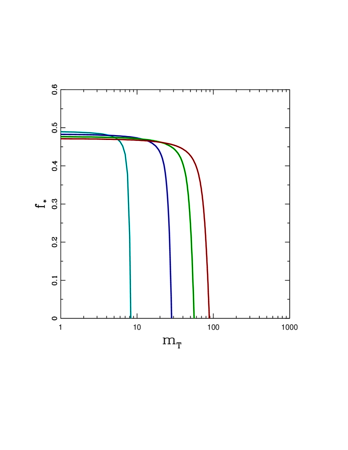
Figure 1: Optimized value of the mass fraction $f$ (of the inner planet) as a function of the total mass $m_{\scriptstyle T}$ of the planetary pair (in units of $M_{\oplus}$). For the sake of definiteness, the stellar mass $M_{\ast}=1M_{\odot}$, the semimajor axis $a_{2}$ = 0.1 AU, and the planet radius $R_{\rm p}$ = 3 $R_{\oplus}$. The four curves correspond to different values of the orbital spacing parameter $\Lambda$ = 1.25 (cyan), 1.5 (blue), 1.75 (green), and 2.0 (red), from left to right in the figure. Note the relatively sharp transition from $f\sim 1/2$ to $f\to 0$ as the total mass $m_{\scriptstyle T}$ increases.

Figure 1 shows the mass fraction $f$ as a function of the total mass $m_{\scriptstyle T}$. Results are shown for four values of the orbital spacing parameter $\Lambda$ = 1.25 – 2, with the remaining parameters the same as those used in the above estimate. The figure shows that the transition from systems with nearly equal mass planets ($f\sim 1/2$) to systems where one planet dominates the mass budget ($f\to 0$) is relatively sharp. The mass threshold for this transition increases with increasing orbital spacing, but is of order tens of $M_{\oplus}$ for the expected (observed) values of the spacing parameter.

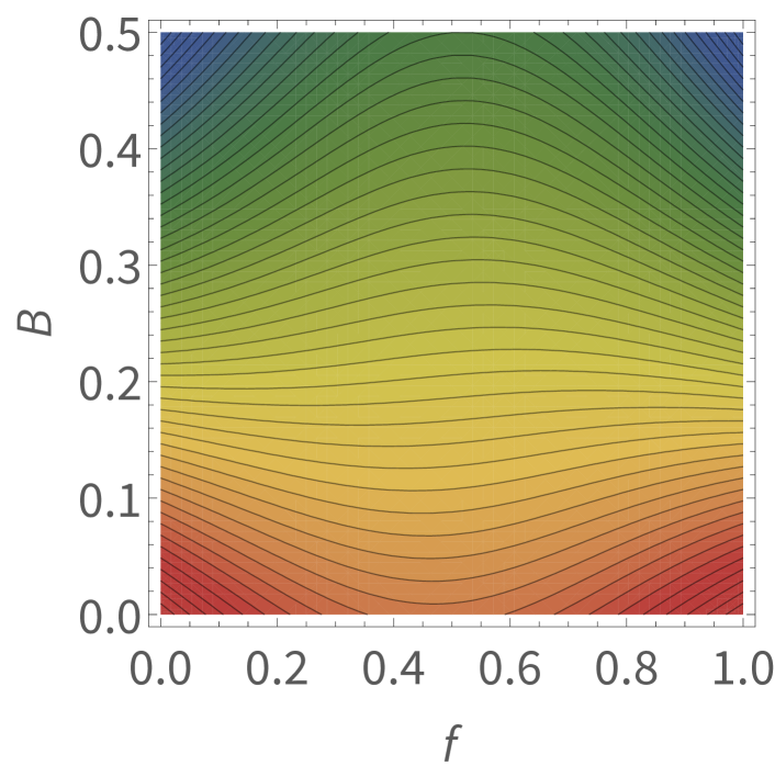
Figure 2: Contour plot showing the energy as a function of the mass fraction $f$ and the dimensionless parameter $B$ that specifies the relative importance of self-gravity of the planets. The orbital spacing parameter $\Lambda=2$. Note that the contours of constant energy are concave upward for small values of $B$, leading to optimized values near $f\sim 1/2$. In contrast, the contours are concave downward for larger $B$, which favors $f\sim 0$ and $f\sim 1$.

Figure 2 shows a contour plot of the energy as a function of the mass fraction $f$ and the parameter $BL^{2}$ that provides a measure of the importance of self-gravity in the system (where we let $BL^{2}\to B$ to simplify the notation). For the sake of definiteness, the orbital spacing parameter $\Lambda$ = 2 for this figure. The contours of constant energy are concave upward for small values of $B$ and transition to concave downward for larger values of $B$. More specifically, the plot shows that we get a well defined minimum at $f\sim 1/2$ (equal planet masses) in the limit $B\to 0$. For larger $B\sim 1$, the minimum becomes a well-defined maximum, and mass fractions $f\to 0,1$ are favored (with the true minimum moving to $f=0$ at the critical value of $B$ as given by equation [20]). However, in the intermediate regime with $B\sim 1/4$, although the minimum value of the energy favors $f\to 0$, the energy difference is small, as depicted by the mostly horizontal contours in the center of Figure 2. As a result, even though the proclivity for equal mass planets disappears for sufficiently large total masses $m_{\scriptstyle T}$ (equivalently $B$), the preference for unequal mass planets remains weak until the total mass $m_{\scriptstyle T}$ becomes significantly larger than the critical value $m_{\scriptstyle C}$ (given by equation [22]).

2.3 Second Variation

The analysis presented in the previous subsection specifies the equilibrium point of the system. In order to show that this critical point corresponds to a minimum of the energy, we must consider the second variation (Hesse, 1872; Abramowitz & Stegun, 1972). As shown above, the first derivative $dE/df$ is a quadratic function of the mass fraction $f$ and can be written in symbolic form

$${dE\over df}=-A\left[f^{2}-bf+c\right]=0\,,$$ (23)

where we choose the sign of the linear term in the square brackets to be negative, and where the coefficients $b$ and $c$ are given by equation (16). As written, the leading coefficient $A\equiv 3(x-1)^{2}(x^{2}-1)/x^{2}>0$. The solution for the extremum is thus given by equation (17). The second derivative takes the form

$${d^{2}E\over df^{2}}=-A\left[2f-b\right]=-\pm A\left[b^{2}-4c\right]^{1/2}\,,$$ (24)

where the expression is evaluated at the critical point in the second equality. The negative root (of the quadratic whose solution [17] specifies the extremum) thus leads to a positive second derivative and hence an energy minimum, whereas the other root corresponds to an energy maximum. As a result, the relevant root is given by

$$f_{\ast}={b-\left[b^{2}-4c\right]^{1/2}\over 2}\,.$$ (25)

Moreover, the mass fraction $f_{\ast}\to 0$ when $c\to 0$, which leads to the critical mass threshold of equation (22).

3 Application to Planetary Systems

The tidal equilibrium states found in the previous section are robust in that they are independent of the dissipation processes that allow planetary systems to evolve toward configurations of lower energy. On the other hand, not all physical systems will achieve their optimal states of minimum energy. In addition, the enforced constraints on the optimization procedure (conservation of angular momentum, constant total mass, and fixed orbital spacing) will not necessarily hold under all circumstances. As a result, we examine the degree to which optimum energy states can be attained by taking into account evolutionary considerations (Section 3.1). We then discuss the conditions required for the underlying assumptions to be applicable (Section 3.2).

In order for the minimum energy states of this paper to apply to observed planetary systems, at least two conditions must hold: The first is that a pair of planets can maintain a constant period ratio $\Lambda$ while changing their radial distance from the star. It is well established that planetary pairs often execute this type of behavior while migrating in (or near) resonance (e.g., see Peale 1976 for a physical explanation of resonant capture and migration). The second requirement – which is more novel – is that the forming planets can jointly apportion the available mass $m_{\scriptstyle T}$ between the two members. In other words, the planets must have some type of agency that allows for the division of the material, where this allocation is carried out so that energy is minimized.

3.1 Evolutionary Considerations

This section outlines an evolutionary scenario to illustrate how forming planetary pairs could realize their minimum energy states as they grow, subject to the two conditions presented above. Keep in mind, however, that the optimized states found above are independent of this or any evolutionary trajectory. Here we consider a forming pair of planets, where both planets can grow by accreting mass from the background circumstellar disk. We are thus implicitly assuming that the planets are formed from the bottom up, through the accumulation of mass, but otherwise invoke no specific mechanism.

At a given time, let the masses of the planets be given by $m_{1}$ and $m_{2}$, where $m_{1}+m_{2}=m_{\scriptstyle T}$, and where the latter quantity is considered to increase with time. Now suppose that an increment of mass $\delta{m}$ is transferred from the disk to the planets. In order to conserve the total angular momentum, before and after the accretion of the new material $\delta{m}$, the following condition must be met

$$\sqrt{a_{i}}\left[m_{1i}+m_{2i}\sqrt{\Lambda}\right]+\sqrt{b}\,\,\delta{m}=\sqrt{a_{f}}\left[m_{1f}+m_{2f}\sqrt{\Lambda}\right]\,,$$ (26)

where the subscripts $i(f)$ denote the initial (final) values, and where $b$ is the semimajor axis of the mass increment before it is accreted by the planets. To conserve total mass, the individual planet masses must obey the condition

$$m_{1i}+m_{2i}+\delta{m}=m_{1f}+m_{2f}\,.$$ (27)

For any allowed final values of the planet masses, the semimajor axis $a_{f}$ can always adjust to satisfy conservation of angular momentum (26) while keeping the orbital spacing $\Lambda$ constant. As a result, the planets change their radial locations at constant $\Lambda$, thereby invoking the first requirement outlined above.

As mass is transferred from the disk to the forming planets, the total mass of the planetary pair increases. If the planets can reach their minimum energy state as they grow, while simultaneously maintaining orbital period commensurability, then for a given mass $m_{\scriptstyle T}$, the individual planetary masses must be given by

$$m_{1}=f(m_{\scriptstyle T})m_{\scriptstyle T}\qquad{\rm and}\qquad m_{2}=\left[1-f(m_{\scriptstyle T})\right]m_{\scriptstyle T}\,,$$ (28)

where the optimized mass fraction $f(m_{\scriptstyle T})$ is a decreasing function of the total mass (see Section 2.2).

The discussion thus far assumes that equation (28) can be satisfied at all stages of evolution. At early times, when the total mass is small $m_{\scriptstyle T}\ll m_{\scriptstyle C}$, the mass fraction $f$ depends only on $\Lambda$, and this balance can be achieved with both planets gaining mass. However, if the total mass exceeds the critical mass, then the optimal mass fraction $f\to 0$, which would imply that the mass of the inner planet $m_{1}\to 0$. But the smaller planet already has some mass at this stage of evolution, so the system cannot achieve its optimal energy state without removing mass from the planet. Instead of losing mass, the inner planet is likely to maintain a constant mass, as determined by its value at this transition point, but stop growing. The other planet then accretes essentially all of the additional mass from that epoch onward. This scenario is illustrated in Figure 3, which shows the masses of both planets as function of $m_{\scriptstyle T}$, where the mass of the inner planet reaches a constant value.

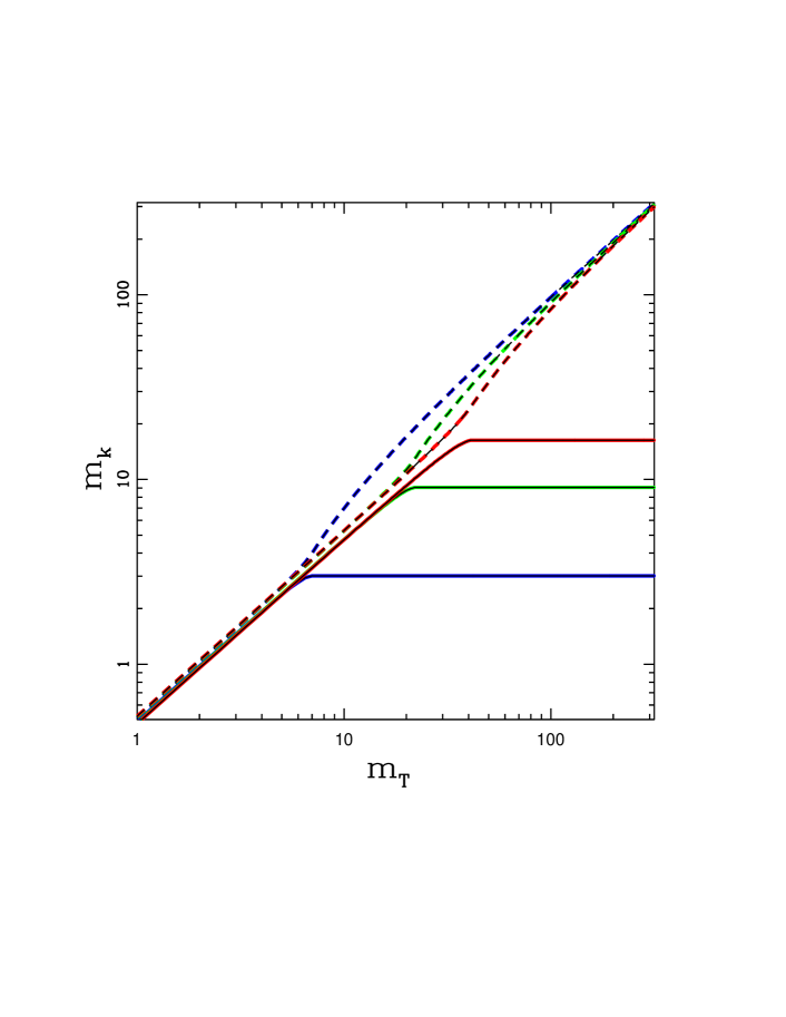
Figure 3: Masses $m_{k}$ of the two members of a planetary pair as a function of the total mass $m_{\scriptstyle T}$, which is considered here to be increasing with time. All masses are given in $M_{\oplus}$. The solid curves show the mass of the inner (smaller) planet, whereas the dashed curves show the mass of the outer (larger) planet. Results are shown for three values of the orbital spacing parameter $\Lambda$ = 1.25 (blue, left), 1.5 (green, middle), and 1.75 (red, right).

In the scenario depicted by Figure 3, the mass of the inner planet reaches an asymptotic value $m_{1}\to m_{\infty}$, which we estimate as follows. The optimum mass of the inner planet $m_{1}$ (from equation [28]) can be considered as a function of $m_{\scriptstyle T}$. The function increases for small values of $m_{\scriptstyle T}$, reaches a maximum, and then decreases for sufficiently large $m_{\scriptstyle T}$ (since $f\to 0$ in the limit $m_{\scriptstyle T}\to m_{\scriptstyle C}$). The point where the inner planet reaches its final mass $m_{\infty}$ is thus given by the condition

$${dm_{1}\over dm_{\scriptstyle T}}=f(m_{\scriptstyle T})+m_{\scriptstyle T}{df\over dm_{\scriptstyle T}}=0\,.$$ (29)

For small values of $m_{\scriptstyle T}$, the mass fraction $f$ is nearly constant, so that the derivative $dm_{1}/dm_{\scriptstyle T}$ is positive. As the total mass approaches the critical value $m_{\scriptstyle T}\to m_{\scriptstyle C}$ (see equation [22]), the quantity $df/dm_{\scriptstyle T}$ becomes large and negative (see Figure 5) while $f$ itself becomes small, so that $dm_{1}/dm_{\scriptstyle T}$ is negative at $m_{\scriptstyle T}=m_{\scriptstyle C}$. In practice, the condition of equation (29) is realized for values of $m_{\scriptstyle T}$ comparable to but somewhat smaller than $m_{\scriptstyle C}$. One can find a closed form solution for the value of $m_{\scriptstyle T}$ at this transition point, but it requires the solution to a cubic equation and the resulting expression is awkward (note that Figure 3 uses the numerical solution). A reasonable approximation can be found by expanding the equations of Section 2.2 to leading order to obtain the expression

$$m_{\infty}\approx{1\over 2}m_{\scriptstyle C}\,\left[1-{1\over 2}\left({\Lambda-1\over\Lambda+2\sqrt{\Lambda}}\right)^{1/2}\right]^{2}\,,$$ (30)

where the critical mass is given by equation (22). This expression for the asymptotic value $m_{\infty}$ for the mass of the inner planet agrees with the full solution to within $\sim 8\%$ for typical planetary systems (those depicted in Figure 3). Note that for late times, the mass fraction in this scenario takes the form $f\to m_{\infty}/m_{\scriptstyle T}$.

In this problem, the quantity $BL^{2}$ represents a control parameter. The critical value from equation (20) is a bifurcation point (Strogatz, 1994), where the preferred state transitions from nearly equal mass planets to one planet dominating the mass supply. However, planetary systems will not always be able to reach their optimal configurations. Consider a system with slowly increasing total mass $m_{\scriptstyle T}$. At a given value of $m_{\scriptstyle T}$, the planets find their optimal configuration, which will have nearly equal masses at early times. In a perfect system, but one with evolutionary constraints, the mass of the smaller planet will stop growing at $m_{\infty}$. In addition, the dynamics of the formation processes (although unspecified in this treatment) will involve some type of time evolution – a flow – for the mass fraction $f(t)$. As the system approaches the bifurcation point ($m_{\scriptstyle T}\to m_{\scriptstyle C}$) from below, this flow is pushing the system toward the equal mass state. After the critical point is reached, this flow continues at first, but it eventually changes after the system becomes sufficiently supercritical. This type of residual behavior, sometimes known as the ‘ghost in the bifurcation’ (Strogatz, 1994), prevents the system from fully realizing its minimal energy configuration, and results in scatter in the resulting system properties.

3.2 Assessment of Assumptions

This optimization scenario of this paper assumes that the forming planets conserve angular momentum and maintain fixed orbital spacing. The calculation also makes implicit assumptions about the relevant time scales. This section examines these assumptions and discusses the conditions necessary for planetary systems to realize these minimum energy states.

In order for the planetary pair to maintain its optimal energy configuration as the bodies grow, the energy dissipation time scale must be much shorter than the time scale for planet formation. Moreover, the two planets must be able to coordinate their mass intake. The natural dynamical time of the system is the orbit time, and any gas in the system communicates through pressure perturbations, which travel at the sound speed. A successful realization of this optimization scheme thus requires the ordering of time scales

$$t_{\rm sc}\sim t_{\rm orb}\ll t_{\rm diss}\ll t_{\rm form}\,,$$ (31)

for the sound crossing, orbital, dissipation, and formation time scales, respectively. The orbit time and sound crossing time are typically a fraction of a year, whereas formation time scales are of order millions of years. As a result, the dissipation time can vary over a relatively wide range and still satisfy the intermediate asymptotic requirement of equation (31).

The optimization procedure of this paper assumes that the planetary pair conserves angular momentum and total mass, while keeping the orbital spacing fixed. Although angular momentum of the entire system is conserved, planet formation takes place within a circumstellar disk containing the planets themselves, along with rocks, dust, and gas. Since the planets under consideration are often super-Earths, they are primarily made of rocky material. More specifically, recent observations (Fulton et al., 2017) indicate that the physical structure of super-Earths is consistent with rocky cores surrounded by low-mass envelopes of hydrogen and helium. As a result, it remains possible for angular momentum of the forming planets to be transferred to the gaseous component, which is eventually removed from the system. The resulting decrease in angular momentum of the planets can lead to migration, which, when paired with planet-planet interactions, can maintain fixed orbital spacing.

In the limit of small total mass $m_{\scriptstyle T}<m_{\scriptstyle C}$, the optimization procedure is independent of the angular momentum (equation [11]), so that $f\approx f_{0}\sim 1/2$ (equation [18]). Decreasing angular momentum leads to an increasing critical mass scale (equation [22]). We thus have the following possible scenarios: If planetary migration is limited, so that $(\Delta a)/a\ll 1$ and hence $(\Delta L)/L\ll 1$, then angular momentum is essentially conserved, any small changes can help maintain the fixed orbital spacing, and the approximations of the previous section are valid. In the case where the planets migrate over longer distances, with larger $(\Delta L)/L$, the critical mass scale $m_{\scriptstyle C}$ increases as the planets move inward. Since the planets start with small masses, where $m_{\scriptstyle T}<m_{\scriptstyle C}$ and $f\approx f_{0}\sim 1/2$, this decreasing angular momentum (increasing critical mass) allows the planets to maintain their well-ordered state (with $f\sim f_{0}\sim 1/2$) over longer times. In this case, the relevant critical mass scale is given by equation (22) evaluated at the final value of $L$ (equivalently $a$). In addition to the ordering of time scales given by equation (31), this scenario requires energy dissipation to occur more rapidly than planetary migration, so that $t_{\rm diss}\ll$ $t_{\rm mig}$.

One can also consider the case where planet formation takes place within a gas-free environment, corresponding to later evolutionary stages. If planetesimals can scatter off of the growing planets, they can be ejected or accreted by the central star, so that the total angular momentum can change in principle. In practice, the planets of interest reside in the inner part of their solar systems, where ejection is suppressed because the required speed is much larger than the escape speed from the planetary surfaces. Ejection will be important for planets forming on sufficiently distant orbits, roughly given by

$$a\,\raise 1.29167pt\hbox{$>$}\kern-7.5pt\lower 3.01385pt\hbox{$\sim$}\,{M_{\ast}\over m_{p}}R_{p}\sim 2\,\,{\rm AU}\,.$$ (32)

Even in the inner solar system, the validity of the optimization procedure requires that the forming planets accrete rocky material with high efficiency, i.e., with little loss from ejection or accretion by the star.

In a gas-free environment, migration can no longer lock planets into mean motion resonance, so that the orbital spacing $\Lambda$ could vary. Numerical simulations show that planets growing within a planetesimal disk will roughly maintain their orbital spacing if they are sufficiently distant, but will experience orbital divergence if the orbits are too close (e.g., Kokubo & Ida 1995). The boundary between these two types of behavior corresponds to separations of $\sim 5$ Hill radii, and results in typical separations of $\sim 10$ Hill radii (Kokubo & Ida, 1998), which is comparable to the observed orbital spacing (Rowe et al., 2014). The results of the optimization procedure vary slowly with changes in the orbital spacing. In the low mass limit, the optimal mass fraction $f_{0}\to 1/2$ in the limit $\Lambda\to 1$ and $f_{0}\to 1/3$ as $\Lambda\to\infty$. The critical mass scale $m_{\scriptstyle C}\propto\Lambda$ in the limit of large $\Lambda$. As result, if planets forming in a gas-free environment increase their orbital spacing due to interactions with planetesimals, the optimum mass fraction will slowly decrease, but the critical mass scale $m_{\scriptstyle C}$ will also increase so that the system tends to remain in the low-mass limit with mass fraction $f\sim f_{0}$. In addition, this scenario allows $m_{\scriptstyle C}$ to plausibly become larger than the local mass budget of solid material.

For completeness, we consider the limiting cases where the constraints are removed entirely. For systems in which angular momentum is not conserved, the lowest energy state is given by the minimum of equation (8), where both the mass fraction $f$ and semimajor axis $a$ can vary. The energy is unbounded from below: The system can always evolve to a lower energy state by moving the planets inward and hence decreasing $a$. This scenario results in all planets being accreted by the central star. In the other case, where the constraint of fixed orbital spacing is removed, the lowest energy state is given by the minimum of equation (11), where the mass fraction $f$ and the spacing $\Lambda$ can vary. In the low mass limit $m_{\scriptstyle T}\ll m_{\scriptstyle C}$, this minimization procedure implies that $\Lambda\to 1$, i.e., the planets are predicted to merge. The complete removal of the constraints thus leads to an optimal configuration with either no planets (no angular momentum constraint) or a single planet (no spacing constraint).

4 Comparison to Observations

The analysis carried out in the previous section suggests that when the total mass $m_{\scriptstyle T}$ of planetary pairs becomes sufficiently large, the preferred value of the mass fraction $f$ switches from nearly equal mass planets with $f\sim 1/2$ to unequal mass planets with $f\to 0$. Previous work has already indicated that the mass uniformity of planetary systems is compromised when the system contains a Jovian planet (Wang, 2017), consistent with these results for systems with large $m_{\scriptstyle T}$. For these high mass cases, since $f\to 0$, the outer planet becomes the larger member of the pair. This finding is also consistent with results for planetary pairs in Kepler multi-planet systems (Ciardi et al., 2013), where the outer planet is more likely to be larger if one or both planets is larger than Neptune. In this section, we look for related observational signatures using the observed mass fractions of planetary pairs.

The observational data used in this section are the same as in Adams (2019). Briefly, the data were extracted from the publicly available exoplanet database, which includes 219 planetary systems with ${\cal N}_{\rm p}\geq 3$ planets, where these systems contain a total of 777 planets. All of the 557 adjacent planetary pairs found in the observational sample are used in this simple analysis (see also Fabrycky et al. 2014; Fang & Margot 2012; Millholland et al. 2017; Petit et al. 2018; Pu & Wu 2015; Rowe et al. 2014; Tremaine & Dong 2012; Wang 2017; Weiss et al. 2018a, b). Systems with only two planets are not included here because they tend to have larger spacing and mutual inclinations, and hence to not display the regularity found in systems with larger ${\cal N}_{\rm p}$. If both planet mass and planet radius are not reported, then the mass is estimated from the observed radius, or the radius is estimated from the measured mass (see Adams 2019 for further detail). One should keep in mind that the mass-radius relation for exoplanets is a multi-valued function (Wolfgang et al., 2016), so that this approach is valid only in a statistical sense.

For all of the planetary pairs in the sample, Figure 4 presents two distributions of the mass fraction $f$. The two histograms in the figure correspond to the low mass and high mass parts of the sample, with $m_{\scriptstyle T}<40M_{\oplus}$ and $m_{\scriptstyle T}>40M_{\oplus}$, respectively. The two distributions are manifestly different. The figure includes the $\sqrt{N}$-errors, marked by error bars, which are smaller than the differences between the two distributions. The distribution for low mass planets shows a significant peak near $f\sim 1/2$, consistent with predictions for systems where the self-gravity of planets is subdominant (equation [18]; see also Millholland et al. 2017; Weiss et al. 2018a). The distribution for high mass planets is nearly flat (within the estimated uncertainties), with slight preferences for the largest and smallest bins (the most unequal mass planets). This latter behavior is expected for systems with sufficiently high total mass $m_{\scriptstyle T}$ (equation [22]; see also Wang 2017).

For completeness, we note that the distributions shown in Figure 4 include planetary pairs of all semimajor axes. However, both the available mass in the original circumstellar disk and the tendency for planetary pairs to experience runaway growth are expected to increase with $a$. Here, the members of the high mass sample span a wide range of semimajor axis, namely 0.15 AU $\leq{a}\leq$ 12 AU. Nonetheless, the mean value of $a$ is larger for the high mass sample ($\langle{a}\rangle\approx 0.71$ AU) than for the low mass sample ($\langle{a}\rangle\approx 0.13$ AU).

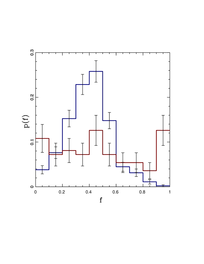
Figure 4: Distribution of mass fraction $f$ for the observed sample of planetary pairs found in extrasolar planetary systems with ${\cal N}_{\rm p}\geq 3$ members. The blue histogram shows the normalized distribution for pairs of low mass planets with total mass $m_{\scriptstyle T}=m_{1}+m_{2}<40M_{\oplus}$. The red histogram shows the corresponding distribution for higher mass planets with $m_{\scriptstyle T}=m_{1}+m_{2}>40M_{\oplus}$. The error bars represent the $\sqrt{N}$-errors. The two distributions are clearly distinct.

The considerations of this paper suggest that planet masses should be comparable for low-mass planetary pairs, but the mass ratios should be much larger for sufficiently high total masses $m_{\scriptstyle T}$. Another way to test this prediction is to plot the observed mass fractions as a function of total mass $m_{\scriptstyle T}$ in the planetary pair, as shown in Figure 5. Since we want to include departures from the case of equal mass planets when either planet is larger, we define an alternative mass fraction $f^{+}$ according to

$$f^{+}\equiv{\rm Max}\left\{f,1-f\right\}\,.$$ (33)

As defined here, this mass fraction must fall in the range $1/2\leq f^{+}\leq 1$.

Figure 5 shows the expected trend that the mass fraction $f^{+}$ for observed planetary pairs increases with total mass $m_{\scriptstyle T}$. For comparison, the theoretically expected mass fraction $f^{+}$ is shown for three values of the (fixed) orbital spacing, $\Lambda$ = 1.25, 1.5, and 1.75, from left to right in the diagram. These curves are calculated from the evolutionary scenario of Section 3.1, where the inner/smaller planet grows as long as it is energetically favorable, but does not decrease its mass. Note that the observed data, depicted as open cyan squares, show a significant amount of scatter. The figure also includes the binned data, shown by the solid black squares with error bars. The binned data indicate that the mass fraction $f^{+}$ is an increasing function of $m_{\scriptstyle T}$. Moreover, the mass fraction increases slowly for small $m_{\scriptstyle T}$, but starts to increase more rapidly for larger total mass $m_{\scriptstyle T}\,\raise 1.29167pt\hbox{$>$}\kern-7.5pt\lower 3.01385pt\hbox{$\sim$}\,40M_{\oplus}$. The observed threshold for mass fraction increases is thus roughly consistent with that of equation (22). Note that the exact shape of the curve shown in Figure 5 depends on the choice of bin size, although the trend of $f^{+}$ increasing with total mass $m_{\scriptstyle T}$ is robust. Moreover, the (binned) observational curve lies above the theoretical values for low masses $m_{\scriptstyle T}\,\raise 1.29167pt\hbox{$<$}\kern-7.5pt\lower 3.01385pt\hbox{$\sim$}\,3M_{\oplus}$ and below for high masses $m_{\scriptstyle T}\,\raise 1.29167pt\hbox{$>$}\kern-7.5pt\lower 3.01385pt\hbox{$\sim$}\,300M_{\oplus}$. This discrepancy indicates that the forming planetary systems do not always reach their optimal energy configurations.

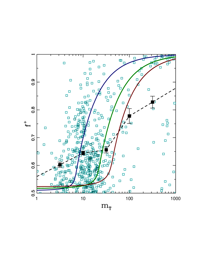
Figure 5: Mass fraction $f^{+}$ of largest planet as a function of total mass $m_{\scriptstyle T}$ of the planetary pair. The alternative mass fraction $f^{+}$ is defined to be $f^{+}=f$ when the inner planet has the larger mass and $f^{+}=1-f$ when the outer planet is heavier. The open cyan squares show the mass fractions for all of the planetary pairs in the observational sample. The solid black squares with error bars show the binned version of the same data. The line dashed connecting the binned data points has been extended to lower and higher masses. The solid curves show the theoretically expected mass fraction $f^{+}$, based on the evolutionary scenario of the previous section, for three values of the orbital spacing parameter $\Lambda$ = 1.25 (left, blue), 1.5 (middle, green), and 1.75 (right, red). Although the data show significant scatter, the mass fraction $f^{+}$ is an increasing function of the total planetary mass $m_{\scriptstyle T}$, especially for $m_{\scriptstyle T}\,\raise 1.29167pt\hbox{$>$}\kern-7.5pt\lower 3.01385pt\hbox{$\sim$}\,40M_{\oplus}$, roughly consistent with the expectations of this paper.

If the masses of the planetary pairs were sampled randomly from a known distribution, then the expected alternative mass fraction $f^{+}$ could be determined and compared with those observed (as shown in Figure 5). Although the underlying mass distribution of the planets is not known, we can illustrate this procedure with a representative example. Suppose that the planetary mass distribution has the form

$${dN\over dm}\propto{1\over m}\qquad{\rm for}\qquad m_{0}\leq m\leq m_{\scriptstyle T}\,,$$ (34)

where $m_{0}$ is the lower-mass cutoff. The actual planetary mass distribution is undoubtedly more complicated, but is subject to a host of selection biases (e.g., Mayor et al. 2011), so its form remains under study. For this distribution, the expectation value of the alternative mass fraction is then given by

$$\langle f^{+}\rangle={\ln(m_{\scriptstyle T}/2m_{0})+m_{0}/m_{\scriptstyle T}\over\ln(m_{\scriptstyle T}/m_{0})}\,.$$ (35)

If we choose $m_{0}=1M_{\oplus}$, under the assumption that smaller planets are not detected in the present sample, then we find that $\langle f^{+}\rangle\approx 0.7$ for $m_{\scriptstyle T}\sim 10M_{\oplus}$ and increases to $\langle f^{+}\rangle\approx 0.9$ for $m_{\scriptstyle T}\sim 100-1000M_{\oplus}$. The expectation value of the mass fraction is thus significantly larger than that observed for low-mass planetary pairs. In contrast, for high-mass pairs, the observed mass fraction approaches the expectation value. As a result, the low-mass pairs show non-random (correlated) masses, consistent with the observational findings that motivated this work. On the other hand, this correlation is compromised for higher total masses, consistent with the theoretical results derived in Section 2.

The moons of the giant planets in our solar system provide another setting for testing the predictions of this energy optimization scenario. The four Galilean moons of Jupiter have nearly uniform masses of $m$ = 0.015, 0.008, 0.025, and 0.018 $M_{\oplus}$, a spread of orbital inclination angles $\Delta{i}<0.5^{\circ}$, and spacing parameters $\Lambda$ = 1.6, 1.6, and 1.8 (from Io on the inside to Callisto on the outside). Moreover, the critical mass predicted from equation (22) is approximately $m_{\scriptstyle C}\approx 0.06-0.07$ $M_{\oplus}$, comfortably larger than the masses of the moons. The Galilean satellite system can thus be understood as a pair-wise equilibrium state. In contrast, the moons of Saturn have non-uniform masses and orbital spacing. The largest body — Titan — dominates the satellite system with mass $m$ = 0.023 $M_{\oplus}$, which is comparable to the critical mass estimated from equation (22), specifically $m_{\scriptstyle C}$ = 0.024 (0.041) $M_{\oplus}$ for the pairing of Titan with Iapetus (Rhea). It is important to stress that the mechanisms that lead to satellite formation are complex; nonetheless, the observed properties are roughly consistent with the optimization scenario considered here.

5 Conclusion

5.1 Summary of Results

This paper determines the lowest energy states available to forming planetary pairs subject to conservation of angular momentum, constant total mass, and fixed orbital spacing. This work generalizes previous treatments by including the self-gravity of the planets in the energy budget (see Section 2). In the limit where the total mass $m_{\scriptstyle T}$ contained in planets is small, the mass fraction of planetary pairs approaches $f\approx 1/2$ (see equation [18]), corresponding to nearly equal mass bodies. As shown previously, this configuration corresponds to circular orbits confined to a single plane, and can be extended to systems with larger numbers of planets (which are then predicted to have nearly equal mass). As the total mass $m_{\scriptstyle T}$ increases, the mass fractions become increasingly asymmetric, and formally $f\to 0$ when the mass $m_{\scriptstyle T}$ exceeds a critical threshold $m_{\scriptstyle T}\,\raise 1.29167pt\hbox{$>$}\kern-7.5pt\lower 3.01385pt\hbox{$\sim$}\,m_{\scriptstyle C}\sim 40M_{\oplus}$ (given by equation [22]). For pairs with larger available mass $m_{\scriptstyle T}$, one planet can thus experience runaway growth, which results in asymmetric masses, and allows for the formation of Jovian planets.

The planetary pairs found in currently observed multi-planet systems have properties that are roughly consistent with the predictions of this energy optimization scenario (see Section 4). Specifically, the masses of members of planetary pairs become more asymmetric as the total mass $m_{\scriptstyle T}$ increases (Figure 5). Similarly, the distribution of mass fractions $f$ shows a clear peak near $f\sim 1/2$ for low-mass pairs with $m_{\scriptstyle T}<40M_{\oplus}$; in contrast, the distribution is nearly flat (uniform) for higher masses $m_{\scriptstyle T}>40M_{\oplus}$ (Figure 4). These observational signatures are consistent with previous work that motivated this analysis, where many systems show nearly equal mass planets on regularly spaced orbits (e.g., Weiss et al. 2018a), whereas systems with large planets break with this relationship (Wang, 2017).

The current data show a significant amount of scatter, and only $\sim 200$ multi-planet systems (with ${\cal N}_{\rm p}\geq 3$) have been detected, so that more observations are necessary to explore these trends in greater detail. Fortunately, new multiple planet systems — and new members — are being discovered and characterized on a regular basis (e.g., see Badenas-Agusti et al. 2020; Feng et al. 2020; Hidalgo et al. 2020; Nielsen et al. 2020; Rodriguez et al. 2020). Such data can be used to update and generalize the correlations depicted in Figure 5. For example, it will be useful to plot the generalized mass fraction $f^{+}$ as a function of the total mass $m_{\scriptstyle T}$ of planetary pairs for various sub-populations as the data become available.

The theory presented in this paper implies several predictions that can be tested in the near-term as the number of detected systems increases, and as the extant system parameters are improved. Such advances will primarily occur through improved planetary mass measurements, but also through detection (via transit timing) of non-transiting planets that occupy apparent gaps in the known multiple-planet systems (see Weiss et al. 2018a, b for some examples). With more and better data, the dependence of $f^{+}$ on $\Lambda$ can be tested, as well as the linear dependence of $m_{\scriptstyle C}$ on $M_{\ast}$ (see equation [22]).

5.2 Discussion

The pair-wise optimization scheme developed here (see also Adams 2019) has important implications for our understanding of extrasolar planetary systems. The lowest energy states available to low-mass planetary systems correspond to nearly equal mass planets on circular orbits, all confined to the same orbital plane. For planetary systems with larger masses, we have shown that it becomes energetically favorable for one planet to dominate the mass supply. It must be emphasized that these results follow from the basic principles of energy minimization, conservation of angular momentum, and conservation of mass (subject to the constraint of fixed orbital spacing). Significantly, these results are independent of the any specific dissipation mechanism and any particular paradigm invoked to explain planet formation, such as Type I migration, pebble accretion, streaming instability, and so on.

This optimization scheme not only explains the so-called peas-in-a-pod properties of the compact multi-planet systems observed by the Kepler mission, but also applies over a wide range of mass scales. The aforementioned systems typically have stellar host masses $M_{\ast}\approx 0.5-1M_{\odot}$ and (nearly) equal mass planets with $m_{\rm p}\sim 10M_{\oplus}$. In contrast, the seven planet system associated with Trappist-1 (Gillon et al., 2016) displays similar uniformity but its mass scales are smaller by an order of magnitude. More specifically, the primary mass $M_{\ast}=0.08M_{\odot}$ and the chain of nearly equal mass planets have $m_{\rm p}\approx 1M_{\oplus}$. As outlined in Section 4, the satellite systems of the giant planets (Galilei, 1610) also display this phenomenon, but the masses are smaller by factors of $\sim 1000$: For example, note that Jupiter has mass $m_{J}=10^{-3}M_{\odot}$ and the Galilean moons have masses of order $m_{\rm gal}\sim 0.01M_{\oplus}$ (equivalently, $10^{-3}\times 10M_{\oplus}$). This phenomenon of regularly spaced, equal mass orbiting bodies thus displays an intriguing degree of universality.

We also note that the giant planets in our solar system exhibit some degree of regularity. Although their total masses vary appreciably, all four planets are thought to have rocky cores with masses $m_{\rm cor}\sim 10M_{\oplus}$ and these bodies exhibit relatively uniform spacing with $\Lambda\approx$ 2, 2, and 3/2 for the three adjacent pairs (using current orbits). According to many models for the early evolution of the solar system (Tsiganis et al., 2005), the giant planets could have formed in a more compact configuration, with tighter orbital spacing $\Lambda\sim 3/2$. However, the critical mass $m_{\scriptstyle C}$ (from equation [22]) decreases with semimajor axis, so that the cores of our giant planets are well above the threshold and probably do not represent a pair-wise equilibrium state.

The concept of energy optimization, with varying individual masses subject to constant total mass, can be applied in other contexts. One interesting setting is that of binary stars. In one classic application (Counselman, 1973; Hut, 1980), energy optimization of binary systems with fixed mass leads to tidal equilibrium states where the rotation rates of both stars are synchronous with the orbital angular velocity, the orbit is circular, and the angular momentum vectors point in the same direction. This problem can be generalized to find the optimal mass fraction for the binary system, analogous to the case considered here for planets. This calculation is beyond the scope of this paper and will be presented elsewhere (Adams et al., 2020).

The basic strategy of this paper is to identify underlying principles — here energy optimization — that specify or constrain the properties of planetary systems. We note that alternate approaches are being developed. As one example, the orbit distribution of observed systems can be described by a statistical model that assumes the systems uniformly sample the stable portion of phase space (Tremaine, 2015). The results of this paper could be used in such a formalism: The ‘temperature’ of the statistical model could be defined in terms of the energy difference between the observed planetary pairs and their minimum energy states (found here).

The results of this paper have a number of additional implications. Given the form of equation (22) for the critical mass, the pair-wise interaction effects considered in this paper favor equal mass planets when they orbit close to their host stars. If the observed Kepler planets, with uniform masses and spacing, had formed in the outer parts of their solar systems and migrated inward, then self-gravity effects could more easily disrupt the pair-wise equilibrium state. For $a\,\raise 1.29167pt\hbox{$>$}\kern-7.5pt\lower 3.01385pt\hbox{$\sim$}\,10$ AU, for example, the threshold mass falls to $m_{\scriptstyle C}\,\raise 1.29167pt\hbox{$<$}\kern-7.5pt\lower 3.01385pt\hbox{$\sim$}\,1M_{\oplus}$, which reflects the fact that gravitational binding energy becomes a progressively more important part of the energy budget with increasing distance from the star. As a result, if this energy optimization scheme provides the explanation for the uniformity of observed compact systems, then in situ formation is favored. A scenario where the range of migration is limited can provide the explanation for the uniform orbital spacing by moving planets toward mean motion resonances, but migration over large distances (see also Section 3.2) is disfavored.

Given that the pair-wise equilibrium states should be less pronounced for outer planets ($m_{\scriptstyle C}$ decreases with increasing $a$), this scenario makes another prediction: The mass fractions $f$ of planetary pairs should favor $f\sim 1/2$ for close orbits and should depart from this uniform state for pairs with increasing semimajor axis $a$. In other words, the peas-in-a-pod phenomenon observed for compact planetary systems should not be prevalent for planets found in larger orbits. This prediction should become testable as the observational sample expands to include planets with longer periods.

Acknowledgments: We would like to thank Juliette Becker, Darryl Seligman, Chris Spalding, and Lauren Weiss for useful discussions. We also thank an anonymous referee for constructive input that improved the paper. This work was supported through the University of Michigan, the National Science Foundation (DMS-1613819), the Air Force Office of Scientific Research (FA 0550-18-0028), NASA (NNX16AB47G), the David and Lucile Packard Foundation, and the Alfred P. Sloan Foundation.

References

- Abramowitz & Stegun (1972) Abramowitz, M., & Stegun, I. A. 1972, Handbook of Mathematical Functions (New York: Dover)
- Adams (2019) Adams, F. C. 2019, MNRAS, 488, 1446
- Adams et al. (2020) Adams, F. C., Batygin, K., & Bloch, A. M. 2020, submitted to MNRAS
- Adams & Bloch (2016) Adams, F. C., & Bloch, A. M. 2016, MNRAS, 462, 2527
- Adams & Bloch (2015) Adams, F. C., & Bloch, A. M. 2015, MNRAS, 446, 3676
- Badenas-Agusti et al. (2020) Badenas-Agusti, M., Günther, M. N., Daylan, T., et al. 2020 arXiv:2002.03958
- Batalha et al. (2011) Batalha, N. M., Borucki, W. J., Bryson, S. T., et al. 2011, ApJ, 729, 27
- Borucki et al. (2010) Borucki, W. J., Koch, D., Basri, G., et al. 2010, Sci, 327, 977
- Chiang & Laughlin (2013) Chiang, E., & Laughlin, G. 2013, MNRAS, 431, 3444
- Ciardi et al. (2013) Ciardi, D. R., Fabrycky, D. C., Ford, E. B., et al. 2013, ApJ, 763, 41,
- Counselman (1973) Counselman, C. C. 1973, ApJ, 180, 307
- Darwin (1879) Darwin, G. H. 1879, The Observatory, 3, 79
- Darwin (1880) Darwin, G. H. 1880, Phil. Trans. R. Soc. A, 171, 713
- Fabrycky et al. (2014) Fabrycky, D. C., Lissauer, J. J., Ragozzine, D., et al. 2014, ApJ, 790, 146
- Fang & Margot (2012) Fang, J., & Margot, J.-L. 2012, ApJ, 761, 92
- Feng et al. (2020) Feng, F., Butler, R. P., Shectman, S. A., et al. 2020, ApJS, 246, 11, arXiv:2001.02577
- Fulton et al. (2017) Fulton, B. J., Petigura, E. A., Howard, A. W. et al. 2017, AJ, 154, 109
- Galilei (1610) Galilei, G. 1610, Sidereus Nuncius; Translated by A. Van Helden 1989, (Chicago: Univ. Chicago Press)
- Gillon et al. (2016) Gillon, M., Jehin, E., Lederer, S. M., et al. 2016, Nature, 533, 221
- Hesse (1872) Hesse, L. O. 1872, Die Determinanten elementar behandelt (Leipzig)
- Hidalgo et al. (2020) Hidalgo, D., Pallé, E., Alonso, R., et al. 2020, A&A, in press, arXiv:2002.01755
- Hut (1980) Hut, P. 1980, A&A, 92, 167
- Kokubo & Ida (1995) Kokubo, E., & Ida, S. 1995, Icarus, 114, 247
- Kokubo & Ida (1998) Kokubo, E., & Ida, S. 1998, Icarus, 131, 171
- Levrard et al. (2009) Levrard, B., Winisdoerffer, C., & Chabrier, G. 2009, ApJ, 692, 9
- Mayor et al. (2011) Mayor, M., Marmier, M., Lovis, C. et al. 2011, arXiv:1109.2497
- Millholland et al. (2017) Millholland, S., Wang, S., & Laughlin, G. 2017, ApJ Letters, 849, L33
- Mills et al. (2019) Mills, S. M., Howard, A. W., Petigura, E. A., et al. 2019, AJ, 157, 198
- Murray & Dermott (1999) Murray, C. D., & Dermott, S. F. 1999, Solar System Dynamics (Cambridge: Cambridge Univ. Press)
- Nielsen et al. (2020) Nielsen, L.D., Gandolfi, D., Armstrong, D. J., et al. 2020, MNRAS, in press, arXiv:2001.08834
- Peale (1976) Peale, S. H. 1976, ARA&A, 14, 215
- Petit et al. (2018) Petit, A., Laskar, J., & Boué, G. 2018, A&A, 617, 93
- Pu & Wu (2015) Pu, B., & Wu, Y. 2015, ApJ, 807, 44
- Rodriguez et al. (2020) Rodriguez, J. E., Vanderburg, A., Zieba, S., et al. 2020, submitted to AAS Journals, arXiv:2001.00954
- Rowe et al. (2014) Rowe, J. F., Bryson, S. T., Marcy, G. W., et al. 2014, ApJ, 784, 45
- Steffen & Hwang (2015) Steffen, J. H., & Hwang, J. A. 2015, MNRAS, 448, 1956
- Strogatz (1994) Strogatz, S. H. 1994, Nonlinear Dynamics and Chaos (Reading: Perseus Books)
- Tanaka & Ward (2004) Tanaka, H., & Ward, W. R. 2004, ApJ, 602, 388
- Tremaine (2015) Tremaine, S. 2015, ApJ, 807, 157
- Tremaine & Dong (2012) Tremaine, S., & Dong, S. 2012, AJ, 143, 94
- Tsiganis et al. (2005) Tsiganis, K., Gomes, R., Morbidelli, A., & Levison, H. F. 2005, Nature, 435, 459
- Van Eylen & Albrecht (2015) Van Eylen, V., & Albrecht, S. 2015, ApJ, 808, 126
- Wang (2017) Wang, S. 2017, RNAAS, 1, 26
- Weiss et al. (2018a) Weiss, L. M., Marcy, G. W., Petigura, E. A., et al. 2018a, AJ, 155, 48
- Weiss et al. (2018b) Weiss, L. M., Marcy, G. W., Petigura, E. A., et al. 2018b, AJ, 156, 254
- Weiss & Petigura (2019) Weiss, L. M., & Petigura, E. A. 2019, arXiv:1908.05833
- Wolfgang et al. (2016) Wolfgang, A., Rogers, L. A., & Ford, E. B. 2016, ApJ, 825, 19
- Zhu et al. (2018) Zhu, W., Petrovich, C., Wu, Y., Dong., S., & Xie, J. 2018, ApJ, 860, 101