Enhancing Physical Layer Security of Random Caching in Large-Scale Multi-Antenna Heterogeneous Wireless Networks
Abstract
In this paper, we propose a novel secure random caching scheme for large-scale multi-antenna heterogeneous wireless networks, where the base stations (BSs) deliver randomly cached confidential contents to the legitimate users in the presence of passive eavesdroppers as well as active jammers. In order to safeguard the content delivery, we consider that the BSs transmits the artificial noise together with the useful signals. By using tools from stochastic geometry, we first analyze the average reliable transmission probability (RTP) and the average confidential transmission probability (CTP), which take both the impact of the eavesdroppers and the impact of the jammers into consideration. We further provide tight upper and lower bounds on the average RTP. These analytical results enable us to obtain rich insights into the behaviors of the average RTP and the average CTP with respect to key system parameters. Moreover, we optimize the caching distribution of the files to maximize the average RTP of the system, while satisfying the constraints on the caching size and the average CTP. Through numerical results, we show that our proposed secure random caching scheme can effectively boost the secrecy performance of the system compared to the existing solutions.
Index Terms:
Physical layer security, random caching, multi-antenna, heterogeneous wireless networks, stochastic geometry, optimization.I Introduction
With the rapid development of wireless technology, the global mobile data traffic is expected to reach 77 exabytes per month by 2022, which is a sevenfold increase over 2017 [1]. However, the majority of such traffic is asynchronously but repeatedly requested by many users at different times and thus a tremendous amount of mobile data traffic has actually been redundantly generated over the mobile networks [2]. Against this backdrop, caching popular contents at the base stations (BSs) has been proposed as a promising approach for shifting the huge mobile data traffic from remote clouds to the edges in mobile networks [3, 4], thereby significantly improving the users’ quality of service (QoS). Motivated by this, cache-enabled wireless networks has recently been attracting great research attention.
However, due to the equipment size and cost issues, the storage resources at BSs are usually limited. Therefore, which contents should be cached at BSs becomes a vital design problem, refereed to as the caching scheme design problem, in cache-enabled wireless networks. In [5, 6, 7, 8, 9, 10, 11, 12, 13, 14, 15], the authors proposed various caching schemes to improve the content transmission reliability (i.e., the probability that the requested content can be successfully transmitted from the BSs to the users, which can reflect the users’ QoS) in large-scale cache-enabled wireless networks. Specifically, in [5], the most popular caching scheme was studied, in which each BS only stores the most popular files. However, such a caching scheme may not yield the optimal network performance, since it cannot provide any content diversity [12, 11, 13]. To tackle this issue, random caching scheme was considered in [6, 7, 8, 9, 10, 12, 11, 13, 14, 15]. More specifically, in [6], the uniform caching was studied, in which, each BS randomly stores a file according to the uniform distribution. In [7, 8, 9, 10, 12, 11, 13, 15, 14], the optimal random caching was examined to maximize the cache hit probability [7, 8], the successful offloading probability [9], and the successful transmission probability [10, 12, 11, 13, 14], or minimize the average caching failure probability [15].
Although significant efforts have been devoted to improve the reliability of content transmission [5, 6, 7, 8, 9, 10, 12, 11, 13, 14, 15], the content transmission secrecy is another important design aspect in the cache-enabled wireless networks, yet receives much less attention. Due to the broadcast nature of wireless communications, the transmissions of the contents cached at BSs are vulnerable to potential eavesdroppers (e.g., non-paying subscribers) and jammers [16, 17, 18]. By attempting to intercept the users’ content transmissions, the eavesdroppers can degrade the confidentiality of content transmissions. By transmitting harmful interfering signal in the wireless networks, the jammers can reduce the reliability of content transmissions. Currently, the most of mobile data services still rely on the traditional cryptographic encryption to guarantee the confidentiality of content transmission. Nevertheless, such encryption creates an insurmountable obstacle to caching content at BSs, since the encrypted content are uniquely defined for each user’s request and cannot be reused to serve other users’ requests [19]. Against this background, physical layer security has been regarded as a promising solution to support caching and enhance the confidentiality of content transmission simultaneously in large-scale cache-enabled single-tier [20, 21] or multi-tier heterogeneous wireless networks (HetNets) [22], due to the fact that it only relies on wiretap channel coding instead of source encryption. In particular, the authors in [20] and [22] proposed a partition-based hybrid caching scheme, where the cache of each BS was partitioned into two halves for storing both the most popular contents and fractions of other contents, and analyzed different physical-layer security performance such as the transmission capacity and energy efficiency [20] as well as the secure content delivery probability [22]. In [21], the authors leveraged the content diversity provided by the random caching to optimize the cache hit probability subject to different content confidentiality level constraints.
The authors in [20, 22, 21] only considered deploying single-antenna at each BS, and therefore, their proposed caching schemes may not achieve desirable security performance in multi-antenna wireless networks. In addition, unlike [20, 22], to deliberately confuse the eavesdroppers, an artificial-noise-aided transmission strategy was further considered in [21]. The key idea of this strategy is to use part of the transmit power at the BS to inject artificial noise into the null space of the legitimate user’s channel, thereby significantly reducing the link quality of the eavesdropper without interfering with the legitimate user [23]. However, since the BSs only have single-antenna, in [21], each BS is only able to transmit either artificial noise or content, resulting in that some users will not be able to download their requested content in a timely manner. Furthermore, it is worth pointing out that the authors in [20, 22, 21] only focused on combating the eavesdropping attack in cache-enabled wireless networks, leading to that their proposed caching schemes may not efficiently resist jamming attack.
In this paper, we would like to address the above issues. We consider a large-scale multi-antenna HetNet employing random caching and artificial-noise-aided transmission strategy, where the BSs deployed at multiple tiers transmit the randomly cached confidential content together with the artificial noise to the legitimate users in the presence of the jammers as well as eavesdroppers. We define and evaluate the content average reliable transmission probability (RTP) and the content average confidential transmission probability (CTP), which characterizes the reliability and the confidentiality of content transmissions, respectively. Our key goal is to determine a secure random caching scheme that maximizes the average RTP under the average CTP and storage resource constraints. Our main contributions are summarized as follows:
-
•
We derive closed-form expressions for the average RTP and CTP in the considered HetNets. Based on which, we further derive tight upper and lower bounds on the average RTP. These analytical results allow us to reveal how the jamming and eavesdropping can have a significant impact on large-scale cache-enabled HetNets.
-
•
We propose a new secure random caching scheme in which the caching distribution of the contents is judiciously determined to maximize the average RTP, while satisfying the constraints on the average CTP and the storage resource.
-
•
Through numerical results, we show that the proposed secure caching scheme outperforms the existing baselines and significantly improves the average RTP, while being resist to the jamming and eavesdropping attack.
Beyond the above contributions, this paper provides valuable insights into the design of secure large-scale cache-enable HetNets. Specifically, we show that, when the constraint on the average CTP is stringent, caching less popular contents at BSs may be helpful for maintaining the level of average RTP. In addition, we show that increasing the cache sizes at BSs does not always improve the average RTP when the secrecy constraint on the average CTP is taken into account.
The rest of the paper is organized as follows. Section II describes the system model and formulates a secrecy performance optimization problem. Section III analyzes the secrecy performance and derives the closed-form expressions for the average RTP and CTP. Based on these analytical results, Section IV develops two algorithms to solve the formulated optimization problem. Numerical results and the related discussions are provided in Section V. Finally, Section VI draws the conclusions. Unless otherwise specified, the notations used throughout the paper are summarized in Table I.
II System Model
II-A Network Model
We consider the secure downlink transmissions in a large-scale cache-enabled HetNet, in which the BSs from co-channel deployed network tiers transmit to the users in the presence of randomly distributed jammers and eavesdroppers. For ease of illustration, we denote the set of tiers by . We assume that each BS in tier is active (as in [8, 10, 12]) and has antennas, while the users, the jammers, and the eavesdroppers are equipped with a single antenna each.111 We understand that the scenario where the users, the jammers, and the eavesdroppers are all equipped with multiple antennas is more general, interesting, as well as challenging. For analytical tractability, we leave it for future work. The eavesdroppers secretly intercept the downlink transmissions, while the jammers constantly broadcast the jamming signals into the channel to interrupt the downlink transmissions. The jammers and the eavesdroppers are not colluding, and therefore the jamming signals also interfere with the eavesdroppers. The BS locations in tier and the jammers are modeled by independent homogeneous Poisson point processes (PPPs) and with densities and ,222In practice, the density of the jammers can be estimated by using the jammer detection policies [24]. respectively. In addition, the locations of the users and eavesdroppers are modeled by some other independent stationary point processes with certain densities.
| Notation | Definition |
|---|---|
| Set of network tiers. | |
| Number of tiers. | |
| Point process of the BSs in tier . | |
| Spatial density of the BSs in tier . | |
| Number of antennas at each BS in tier . | |
| Transmit power of each BS in tier . | |
| Point process of the jammers. | |
| Spatial density of the jammers. | |
| The complex number domain. | |
| Notation representing for user. | |
| Notation representing for eavesdropper. | |
| Small-scale fading vector between BS and receiver . | |
| Small-scale fading coefficient between jammer and receiver . | |
| Path-loss exponent. | |
| Set of files in the network. | |
| Number of files in the network. | |
| Popularity of file . | |
| Popularity distribution of files in . | |
| Cache size of each BS in tier . | |
| Caching probability of file in tier . | |
| Caching distribution of the files. | |
| Point processes of the BSs in tier which store file . | |
| Point processes of the BSs in tier which do not store file . | |
| The information-bearing signal at BS . | |
| The served user of BS . | |
| Artificial noise vector at BS . | |
| Beamforming vector at BS . | |
| The matrix for transmitting the artificial noise at BS . | |
| Fraction of power allocated to the signal . | |
| A typical user. | |
| A typical eavesdropper. | |
| Distance between BS and . | |
| Distance between BS and . | |
| Distance between jammer and . | |
| Distance between jammer and . | |
| Index of the serving BS of in tier . | |
| Index of an arbitrary BS storing file in tier . | |
| Target transmission rate of the wiretap code. | |
| Secrecy rate of the wiretap code. | |
| Redundancy rate against eavesdropping. | |
| A given level of confidentiality. | |
| RTP of file . | |
| Average RTP. | |
| CTP of file . | |
| Average RTP. |
We assume a interference-limited communication environment, in which the wireless channels undergo quasi-static Rayleigh fading along with a large-scale path loss. Specifically, we denote () as the small-scale fading vector (coefficient) between BS (jammer ) and receiver , where denotes the complex number domain, and represent the user and the eavesdropper, respectively. As such, all the entries of and are identical and independent distributed (i.i.d.) circularly symmetric complex Gaussian random variables with zero mean and unit variance. For the path loss model, we use the standard power loss propagation model, i.e., the power of the transmitted signal with distance is attenuated by a factor , where denotes the path-loss exponent.
We consider that there exist files, denoted by the set , to be cached in the considered HetNet. All the files have the same size (as in [7, 9, 12, 8, 10, 11, 13]) and each file has its own popularity (i.e., the probability that file is requested by a user), denoted by , where . Without loss of generality (w.l.o.g.), we assume that . As such, the popularity distribution among can be denoted by , which we assume known a priori. We note that this assumption is practical due to the fact that the file popularity evolves at a slower timescale, thus various methods can be employed to estimate the file popularity over time [25]. We consider a discrete-time system with time being slotted. In each time slot, each user randomly requests one file according to the file popularity . We study one slot in the network.
II-B Random Caching and User Association
We consider that each BS in tier is equipped with a cache unit of size (in files), . As in [7, 9, 12, 8, 10, 11, 13], file is stored at each BS in tier with a certain probability , referred to as the caching probability of file in tier . We denote , where , as the caching distribution of the files in the -tier HetNet. Then, the relationship between the caching probability of file in tier and the cache sizes of the BSs in tier can be expressed as [12, 11, 13]:
| (1) | |||
| (2) |
Let and , denote the point processes of the BSs in tier which store and do not store file , respectively. Then, we have . Due to the random caching and independent thinning [26], we know that and are two thinned and independent homogeneous PPPs with densities and , respectively.
We now describe the user association rule adopted in this paper. Consider a user requesting file at the beginning of a slot. If file is not stored in the HetNet, it will not be served.333Note that in this work, we only study serving cached files at BSs to get first-order insights into the design of cache-enabled -tier HetNets and characterize the benefits of caching, as in [7, 8, 13]. BSs may serve those uncached files through other service mechanisms, the investigation of which is beyond the scope of this paper. Otherwise, it will be associated with a BS which not only stores file but also provides the maximum long-term average received information signal power (ARISP) among all BSs in the -tier HetNet. This BS is referred to as the users’ serving BS and such association mechanism is called the content-based user association. Note that, under this association, a user may not be associated with the BS which provides the maximum ARISP if it has not stored file . As a result, the user usually receives a weak signal compared with the interference, and thus may not successfully receive the requested file and benefit from content diversity offered by random caching. To overcome this drawback, we assume that the channel state information (CSI) of each user is available at its serving BS and the serving BS adopts the maximal ratio transmission to deliver the requested files.444Note that, the analytical framework developed in this paper can be extended to other beamforming techniques.
II-C Artificial-Noise-Aided Transmission
In order to deliberately confuse eavesdroppers in the HetNet while guaranteeing the reliable links to the users, we consider that each BS employs the artificial-noise-aided transmission strategy. Let denote the information-bearing signal with and denote the artificial noise vector at BS . As per the rules of the artificial-noise-aided transmission strategy, all the entries of are i.i.d. circularly symmetric complex Gaussian random variables with zero mean and variance . Then, the transmitted signal from BS can be expressed as
| (3) |
where denotes the transmit power of BS , denotes the fraction of power allocated to the information-bearing signal , is the beamforming vector at BS with representing the served user of BS and denoting the 2-norm of a vector , and is the matrix for transmitting the artificial noise at BS . We choose as the projection matrix into the null space of . As such, the artificial noise will not interfere with user .
II-D Received Signal-to-Interference Ratios
In this paper, w.l.o.g., according to Slivnyak’s Theorem [26], we focus on a typical receiver , located at the origin.555A typical user (eavesdropper) is a user (an eavesdropper) that is randomly selected from all the users (eavesdroppers) in the network. Let () denote the distance between BS (jammer ) and . Based on (3), the received signal at is given by (4), as shown at the top of this page,
| (4) | |||||
where denotes the index of the serving BS of the typical user in tier ,666The serving BS of the typical user is determined according to the content-based user association policy in Section II-B. denotes the index of an arbitrary BS storing file in tier , and denotes the conjugate transpose operation. Then, the SIR at can be expressed as (5), as shown at the top of this page,
| (5) |
where , , and denote the power of artificial noise from BS , the interference and artificial noise from the BSs with storing file in tier , the interference and artificial noise from the BSs without storing file in tier , and the interference from jammers, respectively, given by (6)–(9), as shown at the top of the next page.
| (6) | ||||
| (7) | ||||
| (8) | ||||
| (9) |
Here, is defined as
| (10) |
Note that, we have , ,777Note that means that the random variable follows the distribution . , , and due to the orthogonality between and [27].
Based on (5), the SIR at the typical user can be further written as
| (11) |
where we have and due to . On the other hand, the SIR at the typical eavesdropper can be rewritten as
| (12) |
where we have .
II-E Problem Formulation
According to [28, 29, 30, 31], in order to perform the secure transmission in the considered HetNet, a wiretap code with the parameter pair needs to be constructed, where and denote the target transmission rate and secrecy rate of the wiretap code (both in bps/Hz), respectively. Then the difference is regarded as the redundancy rate against eavesdropping. If the channel capacity between the BS and a user is greater than or equal to , the user is able to decode its desired file. As such, the reliability of file transmission is achieved. If the channel capacity between each BS to an eavesdropper is less than or equal to , the eavesdropper cannot decode any file. In this case, the confidentiality of file transmission is achieved.
Based on the above discussions, we define the reliable transmission probability (RTP) of file as the probability that the transmission of file is reliable. Mathematically, it is given by
| (13) |
Similarly, we define the confidential transmission probability (CTP) of file as the probability that the transmission of file is confidential, which is expressed as (14), as shown at the top of the next page.
| (14) |
Remark 1 (Interpretation of RTP and CTP of file )
The RTP and the CTP of file measure the transmission reliability and the transmission confidentiality of file , respectively. In addition, the RTP (CTP) of file can be thought of equivalently as i) the probability that a randomly chosen user (eavesdropper) succeeds in (fails to) decode file , or ii) the average fraction of users (eavesdroppers) who at any time succeed in (fail to) decode file .
Since each file is requested with probability , according to the total probability theorem, the average RTP and CTP of a file, denoted as and , respectively, are given by
| (15) | |||
| (16) |
where is the design parameter related to random caching.
From (15) and (16), we see that the caching distribution significantly affects both the RTP and the CTP. The key goal of this paper is to optimize to maximize the average RTP of the system, subject to the caching size constraints in (1) and (2) as well as the constraint on the average CTP of the system, given by
| (17) |
where denotes a given level of confidentiality. Mathematically, the optimization problem can be formulated as
Problem 1 (Secrecy Performance Optimization)
where denotes an optimal solution.
III Secrecy Performance Analysis
In order to solve Problem 1, in this section, we analyze and . Specifically, we first derive the closed-form expression of the RTP of file , i.e., . Then, we derive the closed-form expression of the CTP of file , i.e., . Note that, by substituting and into (15) and (16), respectively, we can directly obtain and .
III-A Analysis of RTP
In this subsection, we analyze , using tools from stochastic geometry. To calculate , based on (11), we first need to analyze the distribution of the SIR, . Under random caching, we note that the interferers for the typical user can be classified into three categories, i.e., i) the interfering BSs storing the requested file of in each tier, ii) the interfering BSs without the requested file of in each tier, iii) all the jamemrs in the network. In addition, under artificial-noise-aided transmission strategy, the artificial noise is embedded into the information signal transmitted from each BS in the network. Taking the impacts of these three categories of interferers and the artificial noise on the SIR of the typical user into account, we can derive the distribution of and then , as summarized in the following theorem.
Theorem 1 (RTP of file )
The RTP of file is given by
| (18) |
where is the induced matrix norm and is a lower triangular Toeplitz matrix, i.e.,
| (19) |
Here, , , , where is given by (20), as shown at the top of the next page, with , and given by (21)–(23), respectively, as shown at the top of the next page.
| (20) | ||||
| (21) | ||||
| (22) | ||||
| (23) |
Here, , , and denote the Gauss hypergeometric function and Gamma function, respectively, and and denote the falling and rising factorials, respectively.888Note that when , we define .
Proof: See Appendix A.
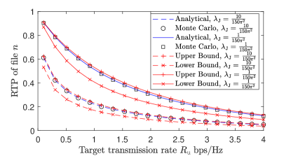
We note that Theorem 1 provides a closed-form expression for . In Fig. 1, we plot versus for different values of . We see that the “Analytical” curves, generated from Theorem 1, accurately match the points obtained from the Monte Carlo simulations, thus verifying the accuracy of the derived expression of in Theorem 1.
Moreover, it is important to understand how is affected by some important system parameters, such as , , , and . In the following, we provide some insights into the behavior of with respect to (w.r.t.) the above parameters. However, due to the induced matrix norm in the expression of , it is extremely difficult to analyze the effects of , , , and . To make progress, we first derive the upper and lower bounds on in the following proposition.
Proposition 1 (Upper and Lower Bounds of RTP of file )
Proof: See Appendix B.
The tightness of and are evaluated in Fig. 1. We can see that and have the similar trends as , which show the correctness of our analysis in Proposition 1. In addition, we see that, compared to , tightly matches , and thus can serve as a good approximation for . Based on Proposition 1, some properties of are established as follows.
Property 1 (Effects of Jammer Transmit Power and Density)
increases with and .
Proof: The proof is straightforward and we omit it for brevity.
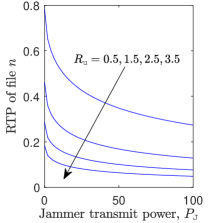
Property 1 indicates that the jammers will degrade the transmission reliability of file , since the jamming signals degrade the link qualities of the typical user’s channels. Fig. 2 plots versus and . From this figure, we see that although Property 1 is obtained based on , it holds for as well. To obtain more insights, we consider a special case where all the BSs have the same number of antennas and power allocation ratio , i.e., and , for all . In this special case, we can further obtain the following properties.
Property 2 (Effects of BS Transmit Power and Density When and , )
When and , for all , increases with and if , and decrease with and otherwise, where is given by (26), as shown at the top of the next page, and
| (26) |
is given by
Proof: Denote . When and , for all , we rewrite (25) as
| (27) |
Then, based on (27), we have
| (30) |
where , and
Finally, by letting and or and , we obtain the desired result in (26), which completes the proof.

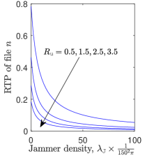
Property 2 indicates that if the caching probability of file in tier is relatively low, then increasing the BS transmit power or density in this tier will decrease the transmission reliability of file . This can be explained as follows. If file is stored in tier with a very low probability, all the BSs in this tier will be the interferer of the typical user. As such, the increase of the BS transmit power or density in tier will increase the interference suffered by the typical user. Fig. 3 plots versus and . From the figure, we see that Property 2 also holds for .
Property 3 (Effect of Caching Probability When and , )
When and , for all , increases with .
Proof: See Appendix C.
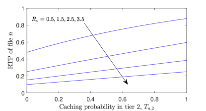
Property 3 indicates that caching a file at more BSs will always increase the transmission reliability of this file. This is because the average distance between a user requesting file and its serving BS decreases with the caching probability . Fig. 4 plots versus , from which we observe that Property 3 also holds for .
Finally, we study the concavity and convexity of and w.r.t. , as follows.
Property 4 (Concavity and Convexity of and w.r.t. Caching Probability When and , )
When and , for all , is a concave function of , and is a difference-of-concave (DC) function of , where
| (31) |
Here, is a concave function of , and denote the sets of the odd and even numbers in set , respectively,
Proof: See Appendix D.
III-B Analysis of CTP
In this subsection, we analyze , using tools from stochastic geometry. To derive , we must derive the joint probability distribution of for all , which, however, is extremely challenging due to the fact that the variables , for all are correlated with each other. In order to make progress, motivated by [32], we focus on the high redundancy rate scenario, i.e., bps/Hz. Note that, it shows in [32, Lemma 1] that in this scenario, at most one BS in the entire network can provide channel capacity greater than , i.e., the typical eavesdropper can successfully decode message from at most one BS. Then, in this scenario, by carefully characterizing the impact of random caching and the artificial-noise-aided transmission strategy on the distribution of , for each , we can derive the distribution of , for each and then , as summarized in the following theorem.
Theorem 2 (CTP of file )
Proof: See Appendix E.
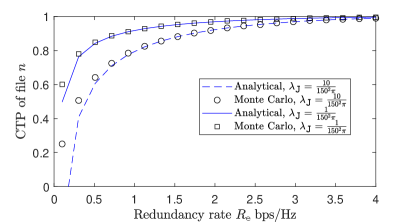
We note that Theorem 2 provides a closed-form expression for in the high redundancy rate scenario. In Fig. 5, we plot versus for different values of . We see that the “Analytical” curves, obtained from Theorem 2, closely match the “Monte Carlo” simulation points, indicating that Theorem 2 can also serve as a good approximation for in the low redundancy rate scenario.
Based on Theorem 2, we can obtain important insights into the behavior of w.r.t the system parameters (e.g., , , , and ), as follows.
Property 5 (Effects of Jammer Transmit Power and Density)
increases with and .
Proof: The proof is straightforward and we omit it for brevity.

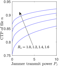
Property 5 indicates that, although the jammers in the HetNets can degrade the transmission reliability of file , they can improve the transmission confidentiality of this file, as shown in Fig. 6. This is because the jamming signals degrade the link qualities of the eavesdropper’s channels.


Property 6 (Effects of BS Transmit Power and Density)
decreases with and if , and increases with and otherwise, where
Proof: The proof is similar to that in Property 2 and we omit it for brevity.
Property 6 indicates that if the caching probability of file in tier is relatively low, then increasing the transmit power or density of the BSs from this tier will increase the transmission confidentiality of file . This is because increasing the transmit power or density of the BSs will result in an increase in the interference received by the eavesdroppers. Fig. 7 verifies Property 6.
Property 7 (Effect of Caching Probability)
decreases with .
Proof: From (2), we have
Obviously, we see that is a constant w.r.t. , which completes the proof of this property .
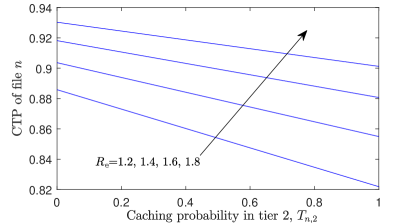
Property 7 indicates that caching a file at more BSs will compromise the transmission confidentiality of this file, since caching the file at more BSs incurs a higher risk of being eavesdropped. Fig. 8 verifies Property 7.
Property 8 (Linearity of w.r.t. Caching Probability)
is a linear function of .
Proof: The proof is straightforward and we omit it for brevity.
In section IV, we shall see that this linearity of will greatly facilitate the performance optimization.
IV Secrecy Performance Optimization
In this section, we focus on solving Problem 1. By substituting (18) into (15) and (2) into (16), the RTP and the CTP are, respectively, calculated as (33) and (34), as shown at the top of the next page.
| (33) | |||||
| (34) |
Recall that the upper bound in (24) provides a good approximation for in (18), and is much more analytical than . Hence, in the following, for simplicity and tractability, instead of maximizing directly, we maximize its upper bound, given by
| (35) |
where is given by (24). As such, we can transform Problem 1 into the following problem
Problem 2 (Simplified Secrecy Performance Optimization)
Problem 2 maximizes a non-concave objective function over a linear set, denoted by , and hence is a non-convex optimization problem in general. Since the objective function is continuously differentiable on , we can obtain a stationary point999Please note that for a non-convex problem, in general, there is no guarantee that an optimal solution can be obtained. Instead, obtaining a stationary point, i.e., a point that satisfies the corresponding Karush-Kuhn-Tucker conditions, is the classic goal for solving a non-convex optimization problem [33]. of Problem 2 by using the gradient projection method (GPM) with a diminishing step size, denoted by with being the iteration index. The details for solving Problem 2 using GPM are summarized in Algorithm 1, where the diminishing step size satisfies , as , and [33, pp. 227]. In addition, in Step 3 of Algorithm 1, denotes the Euclidean projection of onto , and is the gradient of at , given by (IV), as shown at the top of the next page.
| (36) |
Here, and , where , and are given by Theorem 1. According to [34], we know that the sequence generated by Algorithm 1 converges to a stationary point of Problem 2. The computation cost of Algorithm 1 is dominated by the Euclidean projection at Step 3, which has the computational complexity in the use of interior point algorithm [35].
Note that, the convergence rate of Algorithm 1 is sensitive to the choice of the step size. If it is chosen improperly, Algorithm 1 may need a great number of iterations to converge. Recall that in Property 4, in the special case of and , for all , has a DC structure. Thus, in this case, Problem 2 becomes a DC optimization problem and thus can be solved using convex-concave procedure (CCP) [36]. Compared to GPM, CCP does not depend any step size and thus may lead to robust convergence performance. As such, in the following, we consider this special case and develop an iterative algorithm to obtain a stationary point of Problem 2 based on CCP. The core idea of CCP is to linearize the convex term of the DC objective function to obtain a concave objective function for a maximization problem, and then solve a sequence of convex optimization problems successively. Specifically, at iteration , based on Property 4, we have the following approximation problem:
Problem 3 (Approximation of Problem 2 at Iteration When and , )
where , is given by (31) and denotes the gradient of at , which is given by (37), as shown at the top of the next page.
| (37) | |||||
Due to the concave objective and linear constraints, Problem 3 is a convex problem, and thus can be solved by an interior point method efficiently. The details for solving Problem 2 using CCP are summarized in Algorithm 2. To initialize Algorithm 2, we can randomly choose a point and then project it onto the linear constraint set of Problem 2. According to [36], we declare that the sequence generated by Algorithm 2 converges to a stationary point of Problem 2. Similar as Algorithm 1, the computation cost of Algorithm 2 is dominated by the solution of Problem 3 at Step 3 as well, which has the computational complexity in the use of interior point algorithm [35].
V Numerical Results
In this section, we provide numerical results to verify the effectiveness of our proposed secure random caching scheme. Specifically, we first demonstrate the convergence of Algorithm 1 and Algorithm 2. Then, we compare the performance of the proposed secure random caching scheme with that of some existing baseline schemes. In the simulations, we consider a two-tier HetNet, i.e., , consisting of a macrocell network as the 1st tier overlaid with a picocell network as the 2nd tier. Unless otherwise stated, the simulation settings are as follows: , , W, W, W, , , , , bps/Hz, bps/Hz, , , , , , and , where is the Zipf exponent.

V-A Convergence of Algorithm 1 and Algorithm 2
In Fig. 9, we present the convergence trajectories of Algorithm 1 and Algorithm 2 as functions of iteration index for five different initial points. We see that the convergence rate of Algorithm 1 is highly sensitive to the choices of step size, while Algorithm 2 has more robust convergence performance, due to the fact that it does not rely on any step size. We also see that, for different initial points, both Algorithm 1 and Algorithm 2 converge to the same RTP, demonstrating their effectiveness in solving Problem 2. Moreover, compared to Algorithm 2, the convergence trajectory of Algorithm 1 is not monotonically decreasing, due to the Euclidean projection onto the feasible set.
V-B Performance Comparisons between Proposed Scheme and Baselines

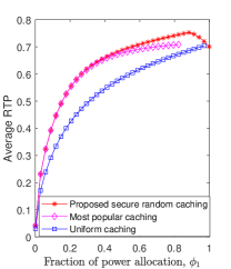
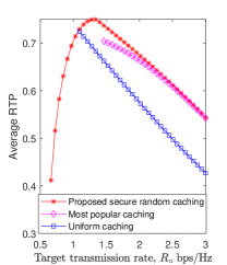
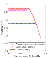
In Fig. 10 – Fig. 13, we examine the effects of system parameters and demonstrate the superiority of our proposed secure random caching schemes over two baseline schemes, in terms of the average RTP. Specifically, Baseline 1 adopts the most popular caching scheme, where each BS in tier selects the most popular files to store [5], and Baseline 2 adopts the uniform caching scheme, where each BS in tier randomly selects files to store, according to the uniform distribution [6].
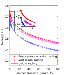
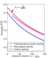
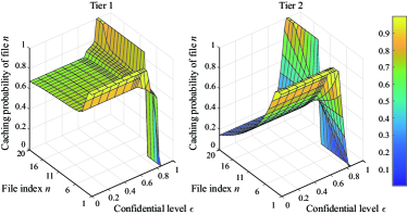
Fig. 10 shows the effect of the confidential level . Specifically, in Fig. 10(a) we plot the average RTP versus . From the figure, we can see that for a large , the two baseline schemes may be infeasible (e.g., for the most popular caching and for the uniform caching), but our proposed secure random caching scheme may still be feasible (e.g., ), at the cost of RTP decrement (e.g., ). This can be explained as follows. The CTPs of the two baseline schemes (each with fixed caching distribution of files) are deterministic if given the system parameters. Therefore, the decrease of the confidential level will easily violate the confidential level constraint in (17). On the contrary, our proposed scheme can wisely adjust the caching distribution of the files to increase the CTP such that the confidential level constraint is satisfied. The corresponding adjustment in caching distribution is illustrated in Fig. 10(b). To be specific, in the region of , a file with higher popularity has a higher caching probability, while in the region of , the caching probability of a file with higher popularity gradually decreases with , which in turn leads to a reduction of the average RTP.
In Fig. 11, we examine the effects of the transmit power and density of the jammers, i.e., and . We first see that the average RTP of each caching scheme decreases as or increases, which verifies Property 1. We also see that, when or is relatively high (e.g., W or ), the most popular caching can achieve almost the same average RTP as our secure random caching. This is because, when or is large, the received SIR at the typical user is small. As such, our secure random caching scheme tends to cache the files with higher popularity in order to provide the largest possible average RTP. In addition, we see that, when or is low (e.g., W or ), the most popular caching may be infeasible, but our secure random caching scheme can still be feasible, demonstrating that compared to the baselines, our proposed scheme can effectively resist jamming attack.
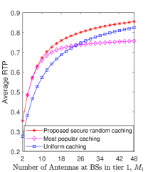
Next, we examine the effects of the number of BS antennas , the power allocation , the target transmission rate , and the secrecy rate in Fig. 12.101010In Fig. 12(a), the operation denotes the ceiling function. We see that, when is small, is low or is large, the most popular caching scheme can achieve almost the same average RTP as our proposed secure random caching scheme, since caching the most popular files at each BS can compensate lower received SIR at the typical user. In addition, we also see that when is large, is small or is large, the two baseline schemes may be infeasible but our proposed schemes may still be feasible, demonstrating that our schemes can well adapt to the changes of these parameters.
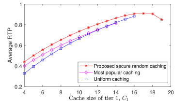
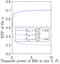
Finally, we examine the effects of the cache size in Fig. 13. From the figure, we can see that, when the cache size is large enough, the baselines may not be feasible, while our proposed scheme can still be feasible, but at the cost of the average RTP decrement. This observation indicates that increasing the cache sizes at the BSs does not always increase the average RTP, which is significantly different from the observations in the existing works without considering the secrecy constraints, e.g., [10, 12, 11, 13]. This can be explained as follows. If the cache size increases, for the most popular caching scheme, each BS will store more files, while for the uniform caching scheme, each file will be stored at more BSs, both of which will increase the risk of eavesdropping, i.e., the average CTP for the two baselines will decrease. If the average CTP is below the given confidential level, the baselines will be infeasible. On the other hand, our proposed secure caching scheme can wisely adjust the caching distribution of the files (i.e., reduce the caching probability of a file with higher popularity as shown in Fig. 10(b)) to maintain the average CTP above the given confidential level. However, such adjustment leads to a reduction of the average RTP.
VI Conclusions
In this paper, we examine the security issue in the cache-enabled large-scale multi-antenna HetNets, in which the multi-antenna BSs deployed at multiple independent network-tiers deliver their cached files to the requesting users in the presence of the eavesdroppers and the jammers. To confuse the eavesdroppers, the BSs transmits artificial noise as well as the useful signals, simultaneously. We first derive closed-form expressions for the average RTP and the average CTP, characterizing the impacts of the eavesdroppers and jammers on the secrecy performance of the system. We then derive closed-form upper and lower bounds for the RTP, which facilitates us to understand the effects of key system parameters. In addition, we propose a secure random caching scheme which optimizes the caching distribution of the files to maximize the average RTP of the system, while simultaneously meeting the requirements on the caching sizes at the BSs and the average CTP of the system. Numerical results show that the proposed secure random caching scheme significantly outperforms the existing baseline solutions.
Appendix A Proof of Theorem 1
| (38) | |||||
where (a) is due to the fact that and is the probability that the typical user is associated with tier ; (b) follows from with denoting the -order derivative of the Laplace transform of random variable , i.e., ; and (c) uses the probability density function (p.d.f.) of the distance , i.e., , which is given by
| (39) |
Thus, to calculate , we only need to calculate .
First, we calculate . Note that we have . In the following, we calculate , and , respectively. Let with the p.d.f. being given by [37, Lemma 1]. We calculate as (40), as shown at the top of the next page,
| (40) | |||||
where (d) follows from the probability generating functional (PGFL) over PPP and is the Laplace transform of ; (e) follows from [38, eq. (49)] and and are, respectively, given by (41) and (42), as shown at the top of the next page, with
| (41) | |||||
| (42) |
. Similarly, and are calculated as (43) and (44), respectively, as shown at the top of the next page.
| (43) | |||||
| (44) |
Based on (40), (43) and (44), we have
| (45) |
where is given by (46), as shown at the top of the next page,
| (46) |
with and .
Next, we calculate . Note that, directly computing the derivatives will lead to intractable expressions. To address this issue, according to [39, Lemma 1], we obtain the following recursive relations
| (47) | |||
where
| (48) |
From (47), we can see that in order to calculate , we only need to calculate , which are related to the derivatives of . As shown in [39], obtaining a closed-form solution for is generally much easier than for . Specifically, we have (49), as shown at the top of this page,
| (49) |
| (50) | |||||
| (51) | |||||
| (52) | |||||
| (53) | |||||
Appendix B Proof of Proposition 1
The lower bound on can be directly obtained by using the Lemma 1 in [40], and thus we omit the details due to page limitation. In the following, we focus on the calculation of the upper bound on . Specifically, based on the derivation in (38), we have (56), as shown at the top of the next page,
| (56) | |||||
where (a) is due to the fact that and is the probability that the typical user is associated with tier ; (b) follows from a lower bound on the incomplete gamma function, i.e., for ; and (c) follows from the binomial expansion. Substituting (A) and (45) into (56) and using some algebraic manipulations, we obtain the upper bound on , as shown in (24). Thus, we complete the proof.
Appendix C Proof of Property 3
| (57) |
where and are given by (22) and (23), respectively. First, it is easy to see that due to . Denote . Then, based on the following Lemma 1, we have . Hence, we have , which completes the proof.
Lemma 1 (Sign of )
We have .
Proof: According to (22), we consider the cases of and , respectively. If , we have and thus holds clearly. If , for ease of illustration, we rewrite as , where is given by (58), as shown at the top of the next page, and . We first show . To be specific, we further rewrite as , where and . Clearly, if , we have due to , , and ; if and is odd, i.e., , we have due to , , and ; if and is even, i.e., , we have due to , , and . Next, we show . Specifically, we have . Thus, if , we still have . By considering both cases of and , we complete the proof.
| (58) |
Appendix D Proof of Property 4
Due to the space limitations, we only prove the property that is a DC function of . Note that the property that is a concave function of can be proved by following similar steps. Denote . By using the definition of in (20), we rewrite as (59), as shown at the top of this page,
| (59) |
where and . Then, we have (60), as shown at the top of this page.
| (60) |
By following similar proof steps for Lemma 1 in Appendix C, one can show that , and , and thus, we have , implying that is concave w.r.t. . Finally, since is an affine mapping of , according to [35], we can conclude that is also a concave function of , which completes the proof.
Appendix E Proof of Theorem 2
Denote , with and . Then, substituting (12) into (14), we have
| (61) |
where (a) follows from the De Morgan’s laws in the generalized form, and denotes the indicator function of the event , which takes value 1 when the event happens and value 0 when the event does not happen; (b) is in general an upper bound (by union bound) but holds with equality if at most one of the BSs can provide channel capacity greater than , which is precisely the case when we consider ; (c) is obtained by using the Campbell Mecke Theorem [26]; and (d) follows from . Thus, to calculate , we only need to calculate . Note that, we have . By following the similar steps as in the derivation of in Appendix A, we have , and
where is given by (41). Then, we have
| (62) |
where and are given by Theorem 1. Substituting (62) into (61), we complete the proof of Theorem 2.
References
- [1] Cisco, “Cisco visual networking index: Global mobile data traffic forecast update 2016-2021, white paper,” Feb. 2017.
- [2] D. Liu, B. Chen, C. Yang, and A. F. Molisch, “Caching at the wireless edge: design aspects, challenges, and future directions,” IEEE Commun. Mag., vol. 54, no. 9, pp. 22–28, Sep. 2016.
- [3] L. Li, G. Zhao, and R. S. Blum, “A survey of caching techniques in cellular networks: Research issues and challenges in content placement and delivery strategies,” IEEE Commun. Surveys Tuts., vol. 20, no. 3, pp. 1710–1732, 2018.
- [4] Y. Fu, W. Wen, Z. Zhao, T. Q. S. Quek, S. Jin, and F. Zheng, “Dynamic power control for noma transmissions in wireless caching networks,” IEEE Wireless Commun. Lett., vol. 8, no. 5, pp. 1485–1488, Oct. 2019.
- [5] E. Baştuĝ, M. Bennis, M. Kountouris, and M. Debbah, “Cache-enabled small cell networks: modeling and tradeoffs.” EURASIP J. Wireless Commun. Netw., vol. 2015, no. 1, pp. 1–11, Feb. 2015.
- [6] S. T. ul Hassan, M. Bennis, P. H. J. Nardelli, and M. Latva-Aho, “Modeling and analysis of content caching in wireless small cell networks,” in Proc. IEEE ISWCS, Brussels, Belgium, Aug. 2015, pp. 765–769.
- [7] B. Blaszczyszyn and A. Giovanidis, “Optimal geographic caching in cellular networks,” in Proc. IEEE ICC, London, UK, Jun. 2015, pp. 3358–3363.
- [8] J. Wen, K. Huang, S. Yang, and V. O. K. Li, “Cache-enabled heterogeneous cellular networks: Optimal tier-level content placement,” IEEE Trans. Wireless Commun., vol. 16, no. 9, pp. 5939–5952, Sep. 2017.
- [9] D. Liu and C. Yang, “Optimal content placement for offloading in cache-enabled heterogeneous wireless networks,” in Proc. IEEE GLOBECOM, Dec. 2016, pp. 1–6.
- [10] K. Li, C. Yang, Z. Chen, and M. Tao, “Optimization and analysis of probabilistic caching in -tier heterogeneous networks,” IEEE Trans. Wireless Commun., vol. 17, no. 2, pp. 1283–1297, Feb. 2018.
- [11] W. Wen, Y. Cui, F. Zheng, S. Jin, and Y. Jiang, “Random caching based cooperative transmission in heterogeneous wireless networks,” IEEE Trans. Commun., vol. 66, no. 7, pp. 2809–2825, Jul. 2018.
- [12] Y. Cui and D. Jiang, “Analysis and optimization of caching and multicasting in large-scale cache-enabled heterogeneous wireless networks,” IEEE Trans. Wireless Commun., vol. 16, no. 1, pp. 250–264, Jan. 2017.
- [13] W. Wen, Y. Cui, F. Zheng, S. Jin, and Y. Jiang, “Enhancing performance of random caching in large-scale heterogeneous wireless networks with random discontinuous transmission,” IEEE Trans. Commun., vol. 66, no. 12, pp. 6287–6303, Dec. 2018.
- [14] D. Jiang and Y. Cui, “Enhancing performance of random caching in large-scale wireless networks with multiple receive antennas,” IEEE Trans. Wireless Commun., vol. 18, no. 4, pp. 2051–2065, Apr. 2019.
- [15] H. J. Kang and C. G. Kang, “Mobile device-to-device (d2d) content delivery networking: A design and optimization framework,” J. Commun. Netw., vol. 16, no. 5, pp. 568–577, Oct. 2014.
- [16] N. Zhao, F. Cheng, F. R. Yu, J. Tang, Y. Chen, G. Gui, and H. Sari, “Caching uav assisted secure transmission in hyper-dense networks based on interference alignment,” IEEE Trans. Commun., vol. 66, no. 5, pp. 2281–2294, May 2018.
- [17] F. Cheng, G. Gui, N. Zhao, Y. Chen, J. Tang, and H. Sari, “Uav-relaying-assisted secure transmission with caching,” IEEE Trans. Commun., vol. 67, no. 5, pp. 3140–3153, May 2019.
- [18] Q. Zhu, W. Saad, Z. Han, H. V. Poor, and T. Baar, “Eavesdropping and jamming in next-generation wireless networks: A game-theoretic approach,” in MILCOM, Nov. 2011, pp. 119–124.
- [19] G. Paschos, E. Bastug, I. Land, G. Caire, and M. Debbah, “Wireless caching: technical misconceptions and business barriers,” IEEE Commun. Mag., vol. 54, no. 8, pp. 16–22, Aug. 2016.
- [20] T. Zheng, H. Wang, and J. Yuan, “Physical-layer security in cache-enabled cooperative small cell networks against randomly distributed eavesdroppers,” IEEE Trans. Wireless Commun., vol. 17, no. 9, pp. 5945–5958, Sep. 2018.
- [21] Q. Yang, H. Wang, and T. Zheng, “Delivery-secrecy tradeoff for cache-enabled stochastic networks: Content placement optimization,” IEEE Trans. Veh. Technol., vol. 67, no. 11, pp. 11 309–11 313, Nov. 2018.
- [22] T. Zheng, H. Wang, and J. Yuan, “Secure and energy-efficient transmissions in cache-enabled heterogeneous cellular networks: Performance analysis and optimization,” IEEE Trans. Commun., vol. 66, no. 11, pp. 5554–5567, Nov. 2018.
- [23] W. Wang, K. C. Teh, K. H. Li, and S. Luo, “On the impact of adaptive eavesdroppers in multi-antenna cellular networks,” IEEE Trans. Inf. Forensics Secur., vol. 13, no. 2, pp. 269–279, Feb. 2018.
- [24] W. Xu, W. Trappe, Y. Zhang, and T. Wood, “The feasibility of launching and detecting jamming attacks in wireless networks,” in Proc. MobiHoc, ser. MobiHoc ’05. New York, NY, USA: ACM, 2005, pp. 46–57.
- [25] K. Shanmugam, N. Golrezaei, A. G. Dimakis, A. F. Molisch, and G. Caire, “Femtocaching: Wireless content delivery through distributed caching helpers,” IEEE Trans. Inf. Theory, vol. 59, no. 12, pp. 8402–8413, Dec. 2013.
- [26] M. Haenggi, Stochastic Geometry for Wireless Networks. Cambridge, U.K.: Cambridge University Press, 2012.
- [27] H. Wang, T. Zheng, J. Yuan, D. Towsley, and M. H. Lee, “Physical layer security in heterogeneous cellular networks,” IEEE Trans. Commun., vol. 64, no. 3, pp. 1204–1219, Mar. 2016.
- [28] A. D. Wyner, “The wire-tap channel,” Bell Syst. Tech. J., vol. 54, no. 8, pp. 1355–1387, Oct. 1975.
- [29] M. Bloch and J. Barros, Physical-Layer Security. From Information Theory to Security Engineering. Cambridge: Cambridge University Press, 2011.
- [30] C. Liu, N. Yang, J. Yuan, and R. Malaney, “Location-based secure transmission for wiretap channels,” IEEE J. Sel. Areas Commun., vol. 44, no. 7, pp. 1458–1470, Jul. 2015.
- [31] C. Liu, J. Lee, and T. Q. S. Quek, “Safeguarding UAV communications against full-duplex active eavesdropper,” IEEE Trans. Wireless Commun., vol. 18, no. 6, pp. 2919–2931, Jun. 2019.
- [32] H. S. Dhillon, R. K. Ganti, F. Baccelli, and J. G. Andrews, “Modeling and analysis of k-tier downlink heterogeneous cellular networks,” IEEE J. Sel. Areas Commun., vol. 30, no. 3, pp. 550–560, Apr. 2012.
- [33] D. P. Bertsekas, Nonlinear Programming, 2nd ed. Belmont, MA: Athena Scientific, 1999.
- [34] D. P. Bertsekas, Convex Optimization Algorithms, 1st ed. Athena Scientific, 2015.
- [35] S. Boyd and L. Vandenberghe, Convex Optimization. New York, NY, USA: Cambridge university press, 2004.
- [36] T. Lipp and S. Boyd, “Variations and extension of the convex–concave procedure,” Optim. Eng., vol. 17, no. 2, pp. 263–287, Jun. 2016.
- [37] X. Zhang, X. Zhou, and M. R. McKay, “Enhancing secrecy with multi-antenna transmission in wireless ad hoc networks,” IEEE Trans. Inf. Forensics Secur., vol. 8, no. 11, pp. 1802–1814, Nov 2013.
- [38] W. Wang, K. C. Teh, and K. H. Li, “Artificial noise aided physical layer security in multi-antenna small-cell networks,” IEEE Trans. Inf. Forensics Secur., vol. 12, no. 6, pp. 1470–1482, Jun. 2017.
- [39] X. Yu, C. Li, J. Zhang, M. Haenggi, and K. B. Letaief, “A unified framework for the tractable analysis of multi-antenna wireless networks,” IEEE Trans. Wireless Commun., vol. 17, no. 12, pp. 7965–7980, Dec. 2018.
- [40] C. Li, J. Zhang, and K. B. Letaief, “Throughput and energy efficiency analysis of small cell networks with multi-antenna base stations,” IEEE Trans. Wireless Commun., vol. 13, no. 5, pp. 2505–2517, May 2014.